Extracting the electro-magnetic pion form factor from QCD in a finite volume
Abstract
We consider finite volume effects on the electromagnetic form factor of the pion. We compute the peudoscalar-vector-pseudoscalar correlator in the expansion of chiral perturbation theory up to the next-to-leading order and find a way to remove the dominant part, which comes from a contribution of the pion zero-mode. Inserting non-zero momentum to relevant operators (or taking a subtraction of the correlators at different time-slices), and taking an appropriate ratio of them, one can automatically cancel the zero-mode’s contribution, which becomes non-perturbatively large in the regime. The remaining finite volume dependence, which comes from the non-zero momentum modes, is shown to be perturbatively small even in such an extremal case. Since the zero-mode’s dominance is universal in any finite volume scaling, and we do not rely on any particular feature of the expansion, our method has a wide application to many other correlators of QCD.
I Introduction
The electro-magnetic form factor of the charged pions is one of the fundamental low-energy quantities in Quantum Chromodynamics (QCD). Experimentally, it is related to the pion charge radius through the relation
| (1) |
where denotes the electro-magnetic form factor at the momentum transfer . In terms of chiral perturbation theory (ChPT), it is related to the low-energy constant (or in the case), which appears at the next-to-leading order (NLO) in the chiral Lagrangian Gasser:1983yg ; Gasser:1984gg .
However, it is still a non-trivial task for lattice QCD to fully reproduce or understand the low-energy behavior of the pion form factors. In fact, the lattice data of the pion charge radius have been sizably lower than the experimental value (see the recent review in Brandt:2013ffb ). It is only recently that consistent values of were reported by simulations near the physical point Koponen:Lat2013 ; JLQCD:Latt.2012PoS ; Fukaya:2014jka . According to ChPT, it is known that the pion charge radius shows a logarithmic divergence as the pion mass goes to zero. Thus, we may recognize that our simulated pion masses are too large to reproduce the logarithmic divergence, unless we directly simulate QCD near the chiral limit. Namely, in order to examine the chiral logarithm of the pion charge radius, it is essential to simulate lattice QCD in the very vicinity of the chiral limit.
Although current computational resources allow us to simulate QCD near the physical point, one should carefully take two sources of systematic effects into account in such simulations. One is the cut-off effects, especially those come from breaking of the chiral symmetry. When the simulated quark mass is as small as the typical breaking scale of the chiral (flavor) symmetry (it is typically for the improved Wilson or staggered fermions, where is the QCD scale and denotes the lattice spacing), it is known that the chiral logarithm is largely distorted. The low-lying Dirac eigenvalue spectrum, for example, is a quantity sensitive to such discretization effects Kieburg:2013xta .
Another source which may change the chiral behavior is the finite size of the lattice volume. In the literature, it is often mentioned that the lattice size should satisfy , where is a simulated pion mass Aoki:2013ldr , to suppress the finite size effect at a few % level. Since the computational cost for inverting the Dirac operator increases as decreases, it is demanding to keep to be large enough. Especially when we want to keep a good chiral symmetry to avoid the former discretization effects on the chiral logarithm, and use a fermion formulation such as overlap or domain-wall fermions, the available range of is quite limited.
This naive criterion about , however, comes from the fact that the zero-momentum mode of pions can propagate wrapping around the lattice volume, whose contribution is typically given by . For the excited pion states, the finite volume effects are much smaller, since their discrete energy satisfies in a finite volume, and . Therefore, if we can eliminate or reduce the dominant contribution from the pion’s zero-momentum mode, one should be able to extract the low-energy quantities even on a small lattice.
In this work, we consider the “worst” case, the so-called regime of QCD, to show that the above strategy actually works even in such an extremal situation. In the regime, , and the finite volume effects are generally % and we receive a non-perturbatively large correction from the pion zero-mode. However, using the expansion of ChPT Gasser:1986vb , we compute the pseudoscalar-vector-pseudoscalar three-point function, and find a way to automatically cancel the dominant part of them. Since the zero-mode contribution has no space-time dependence, two simple steps are enough to achieve this:
-
1.
inserting non-zero momenta to relevant operators (or taking a subtraction of the correlators at different source points when one or two of the inserted momenta are zero).
-
2.
taking ratios of them.
We also compute the NLO corrections and show that these effects are actually suppressed by , where denotes the pion decay constant. The preliminary result of this work has already appeared in Ref. Fukaya-Suzuki , and applied to numerical works by JLQCD collaboration JLQCD:Latt.2012PoS ; Fukaya:2014jka .
Here, we would like to remark the difference of our new approach from the conventional ones in the regime. In the previous works, the expansion was used to disentangle the low-energy constants Hansen:1990un ; Hansen:1990yg ; Hernandez:2002ds ; Giusti:2004an ; Bernardoni:2008ei ; Hernandez:2008ft ; Aoki:2011pza , using a bunch of Bessel functions, from the lattice data which were largely contaminated by the finite volume effects. In this work, we use (the expansion of) ChPT in more indirect way : just for finding the combination of the correlators which has a small sensitivity to the volume. As we will see in the following sections, this idea makes the analysis in the regime of QCD greatly simplified. In particular, we would like to emphasize that there is essentially no need to use Bessel functions for the computation of the pion form factor. Moreover, since the dominance of the pion zero-mode’s contribution (having the longest correlation length), is universal for any finite volume effects on any operators, we expect a wide application of this method. It may be useful for heavier hadron form factors, and simulations in the regime as well.
The rest of this paper is organized as follows. In Sec. II, we review the expansion of ChPT and present how to compute the correlators at one-loop level. In Sec. III, we consider the two-point functions to illustrate our new idea. Then, our main result for the pseudoscalar-vector-pseudoscalar three-point functions is presented in Sec. IV, including the NLO effects. In Sec. V, we show how to extract the pion vector form factor, and estimate the remaining finite volume effects numerically : we find that it is a few percent level already at . Summary and conclusion are given in Sec. VI.
II The expansion of ChPT
In this section, we review the expansion of ChPT, and show how to perform the one-loop level calculation of the correlators. First, we give the counting rule of the expansion. Second, we write down the chiral lagrangian with pseudo-scalar and vector source terms, and explain a general procedure to calculate correlators from a partition function. Finally, we give the technical details of this study at the end of this section.
II.1 The chiral Lagrangian
We consider -flavor ChPT in an Euclidean finite volume with the periodic boundary condition in every direction. The Lagrangian Gasser:1983yg ; Gasser:1984gg is given by
| (2) |
where denote the chiral field which is an element of the group . is the chiral condensate and is the pion decay constant both in the chiral limit. The terms omitted by ellipses are the ones at the higher orders. For simplicity, we take the quark mass matrix degenerate and diagonal: .
In the regime Gasser:1986vb , the vacuum is not fixed but has non-perturbatively large fluctuations. Namely, the zero-mode of the pions must be integrated exactly. Thus, we separate it from the non-zero momentum modes and parametrize the chiral field as
| (3) |
where denotes the zero-modes. The non-zero momentum mode is decomposed as with generators , for which we use the normalization of . Since the constant modes are separated from fields as , a constraint
| (4) |
must be satisfied to avoid the double-counting of the zero-modes.
Now, we rewrite the chiral Lagrangian Eq. (2) with the expansion, whose counting rule is given by
| (5) |
as
| (6) | |||||
From this Lagrangian, one can recognize that we are treating a hybrid system containing bosonic fields and a matrix , which are weakly interacting.
For fields, one can perform the Gaussian integrals without difficulty. In this work, we use the correlator in quark-line basis,
| (7) |
where the second term comes from the constraint , and
| (8) |
describes the propagation of the massless bosons. Here, the summation is taken over the non-zero 4-momentum with integers , except for , because of the constraint Eq. (4).
While fields are treated perturbatively, the zero-mode denoted by has to be non-perturbatively integrated (we will denote it by ). It is known that these matrix integrals are expressed by the Bessel functions Leutwyler:1992yt ; Splittorff-Verbaarschot ; Fyodorov-Akemann , which is a peculiar feature of the regime. Historically, this special feature of the regime is used for extracting the leading LEC’s, and , which are more sensitive to the volume than others. However, for the other LEC’s at NLO, we should take a different strategy, or we should remove the contamination from the finite size. In this work on the vector form factor of pions, which is related to , the integral plays a less important role.
II.2 Partition function and correltors
In this subsection, we consider the partition function of ChPT in the regime and show how to calculate the correlation functions. First, we introduce the relevant source terms to the chiral Lagrangian Eq. (2). Since the Lagrangian is invariant under the chiral rotation,
| (9) |
the vector or axial vector operators are given through the Noether’s theorem for the vectorlike transformation and the axial one . It is easy to see that adding these operators is equivalent to replacing the derivatives by the “covariant” derivatives:
| (10) |
where and denote the vector and axial-vector sources, respectively. Similarly, since the Lagrangian is invariant under the Parity transformation,
| (11) |
adding a scalar and a pseudoscalar is absorbed in the mass matrix:
| (12) |
where and denote the scalar and pseudoscalar sources, respectively. we set in the following.
Next, let us introduce the NLO terms of the chiral lagrangian. However, some of them are irrelevant to our calculations. In this study, it is enough to consider the terms with the low-energy constants (). Namely, we consider the Lagrangian
| (13) | |||||
where
| (14) |
The calculation of ChPT is performed in the functional integral formalism. The partition function is defined by
| (15) |
and the correlators are computed by differentiating it with respect to the corresponding sources, and take their zero limits. The pseudoscalar two-point function, for example, is given by
| (16) |
where denotes the coefficient of an generator , where we decompose the source as .
One should note that our non-trivial parametrization of needs a non-trivial Jacobian in the functional integration measure:
| (17) |
A perturbative calculation Hansen:1990un ; Bernardoni:2007hi has shown
| (18) |
which can be regarded as an additional mass term of the fields at the one-loop level. Note that this additional mass doesn’t vanish even in the limit, which keeps the theory infra-red finite.
Finally, let us consider the vacuum and fixing topology. In the regime, we often consider a fixed topological sector, rather than the full QCD vacuum with the vacuum angle . For this purpose, we encode the non-zero vacuum angle to the mass term Aoki:2009mx ,
| (19) |
using the axial rotation. Then we can perform a Fourier transformation with respect to to obtain the partition function at fixed topology,
| (20) |
where denotes the topological charge of the original gauge fields. It is known that this integral can be absorbed in the group integration of the zero-mode: redefining the zero mode,
| (21) |
where , the zero-mode part of the functional integral is modified to
| (22) |
where we have used the fact that the zero-mode in the Lagrangian always appears as a function of (and its Hermitian conjugate). Fixing the topology is technically easier since the group integral is simpler than that of . It is also useful for investigating the finite volume physics which is sensitive to the topology of the gauge fields. It is important to note that the fixing topology effect is totally encoded in the pion-zero mode, and therefore, is automatically eliminated once the effect of the latter is eliminated. Since we will be able to cancel the effect of (from the LO contribution), in the following sections, we don’t distinguish and unless explicitly stated.
We are now ready for the 1-loop computations. However, we would like to give some useful technical details which simplify the calculations, in the next subsection.
II.3 Technical details
Because of the non-trivial parametrization of the chiral field, we have a lot of diagrams to be computed in the expansion of ChPT even at NLO. Here we rewrite the Lagrangian using the non-self-contracting (NSC) vertices, and compute some of 1-loop diagrams in advance, as corrections to the chiral Lagrangian. This reduces the number of diagrams and simplify our calculation.
The -point NSC vertex is defined by
| (23) |
and we can absorb the contracted part in the redefinition of the lower dimensional terms in the Lagrangian. Note that by definition. For example, a term in the Lagrangian at NLO can be re-expressed by
| (24) | |||||
where
| (25) |
can be absorbed in the re-definition of the mass term, and
| (26) |
can be absorbed in the re-definition of the kinetic term. Here, and in the following, the momentum summations in embeded in etc. are kept unperformed until the very end of the calculation, except for the trivially clear cases like , . In this work, we employ the dimensional regularization for the loop integrals.
With the NSC vertices, the action is expanded as
| (27) |
where
| (28) | |||||
| (29) |
where
| (30) | |||||
| (31) |
Note that the linear term in disappears because of the constraint Eq. (4).
Here, the source operators are given by
| (32) | |||||
| (33) | |||||
where
| (34) | |||||
| (35) | |||||
| (36) | |||||
| (37) | |||||
| (38) | |||||
| (39) | |||||
| (40) |
In the above expression, the argument of is omitted for simplicity. In this work, we don’t consider contact correlators at the same position, such as . We have, therefore, only collected the terms linear in the sources and .
Here we note that except for , we can absorb all the factors into the redefinition of the wave functions ( fields), or the coupling constants, by defining
| (41) | |||||
| (42) | |||||
| (43) |
Therefore, except for the 4-th term in Eq. (32), the vertex corrections of the two-point and three-point correlators can be obtained by simply replacing the coefficients of the LO results with the shifted ones and , except for multiplying the coefficient of the second term in ,
| (44) |
and the third term in ,
| (45) |
With this action, for any operator (as a function of and ) in the expansion,
| (46) |
its expectation value is perturbatively evaluated as,
where we have used the following notations,
| (48) | |||||
| (49) |
Note that, due to the use of NSC vertices, we don’t need to calculate the fourth term in Eq. (II.3) since .
In the usual vacuum, denotes a Haar measure on , while it should be replaced by on , for a fixed topological sector as discussed in the previous subsection.
III Two-point functions
As we have mentioned in Sec. I, the dominant finite volume effect on correlators comes from the pion zero-mode. Since the zero-mode itself does not depend on the space-time position , its effect always appear as an -independent constant term or overall constants of -dependent terms. In either case, it is not difficult to eliminate these zero-mode’s effects from the correlators. In this section, we demonstrate this new idea taking the two-point pseudoscalar correlators, as an easiest example.
III.1 LO calculation
Let us consider a pseudoscalar operator in the charged pion channel,
| (50) |
From the chiral symmetry, it is easy to confirm that its two-point function satisfies
| (51) |
and
| (52) |
The quark field basis is convenient unless we consider the neutral sector of ChPT, since shares the same normalization of the so-called “connected” contribution of the conventional meson correlators in lattice QCD. Therefore, we use rather than the original in the following analysis.
Now we can write down the two-point function to ,
| (53) |
where
| (54) | |||||
| (55) |
Note that some NLO contribution is already involved in or since we have resummed the Lagrangian with NSC vertices.
This correlator in Eq. (53) is a known result in the literature, and one can find how to evaluate and in, for example, Ref. Bernardoni:2008ei . In particular, the and –independent constant term is known as a special feature of the regime, and can be used for extracting . In this work, however, we will eliminate this constant term in the end of the calculation. Therefore, we have to treat the second term of Eq. (53) as the LO contribution, and the calculation at one order higher is needed.
III.2 NLO calculation
Next, let us compute the NLO contribution. Here and in the following, we simply neglect the contribution to the constant part.
For the third term of Eq. (II.3), we have
| (56) | |||||
where , and the dimensionless integral part is given by
| (57) | |||||
| (58) | |||||
| (59) | |||||
| (60) | |||||
| (61) | |||||
where . Here we have given more general results than our set-up in this work: with non-degenerate –flavor quark masses ’s. The degenerate results can be obtained simply taking in the above formulas. Note that we have neglected trivially vanishing matrix elements like for .
To summarize our results, it is useful to define the “massive” propagator,
| (65) |
and noting for ,
| (66) |
the correlator in a simple form is obtained,
| (67) | |||||
where denotes the constant term we have omitted, and
| (68) |
The second term of Eq. (67) looks almost the same as the conventional massive pion propagator in the regime. In fact, we can smoothly obtain this by taking the limit where one obtains , , and .
The third term of Eq. (67) is another peculiar term in the regime, which originally comes from a 3-pion state, consisting of one having zero momentum and two having non-zero momenta. At this order, it looks a propagation of two massless particles. However, these propagators should have mass corrections at higher orders, at least, the one from the measure term in Eq. (18), We expect that it cannot reach a long-distance, compared to the single particle propagation. In the following analysis, we simply neglect this NLO term and similar terms in the three-point functions. This truncation may be numerically justified by carefully checking the plateau of the effective mass, when we simulate lattice QCD Fukaya:2014jka .
III.3 Removing dominant finite volume effects in the expansion
Now we are ready to cancel the dominant volume effects. First, we insert spacial momentum to the operators. Namely, we consider
| (69) |
where is the temporal element of , , and is the 3-dimensional momentum. Then, the unwanted constant contribution automatically disappears for . It is also intuitively reasonable that the higher energy states having momenta are less sensitive to the finite volume effects. Even in the case of , it vanishes in a simple subtraction with respect to time: with a reference time-slice .
The second step is to take a ratio of the correlators with different momenta. For example, by shifting , and renaming , we have
where
| (71) |
The ratio is no more dependent on or . In fact, this expression is exactly the same as the same ratio in the expansion, except for the mass renormalization factor . Namely, we have minimized the features of the regime in the two-point correlator. It is also important to note that is finite even in the limit of .
Since the above ratio has no dependence on LEC’s of ChPT, it is not phenomenologically interesting. However, it is a good test quantity for lattice QCD to check the validity of the above arguments. Recently, JLQCD collaboration Fukaya:2014jka compared the ratio to the numerical data in the both cases with and 100 MeV and found a fairly good agreement, which suggests that the NLO corrections in and the third term of Eq. (67) we have neglected are actually small.
Since the -independence of the pion zero-mode and its dominance in the finite volume effects are universal and true in any correlation functions at any sizes of the volume, we expect wide applications of our method. Namely, inserting momenta to the correlators and taking a ratios of them generally makes a less sensitive quantity to the volume than the original ones. We will see this is true for the three-point functions in the next section.
IV Three-point function
In this section, we calculate our main target, the pseudoscalar-vector-pseudoscalar three-point function in a finite volume in the expansion of ChPT, which is relevant for extracting the vector pion form factor. However, we should note that the pion form factor itself is not a quantity described within ChPT alone. In numerical studies Aoki:2009qn ; Kaneko:2010ru it is known that the vector meson largely contributes to the results, which cannot be explained by ChPT. Even in such a case, we still expect that the correction from the finite volume can be treated within ChPT, as the heavier hadrons, including the vector mesons, do not propagate very long. Therefore, in this section, we compute the finite volume effects on the three-point function within the expansion of ChPT. Once the main part of finite volume effects are removed, the remaining pion form factor should include the physics beyond ChPT.
IV.1 Three-point functions and form factors
First, we briefly review how the three-point functions are related to the pion form factors. Our main target in this work is the vector form factor, defined by
| (72) |
where denotes the on-shell pion state with momentum , is the coefficient of an generator in the vector operator, and .
For lattice QCD calculations, it is convenient to take component
| (73) |
Using a conventional notation
| (74) |
where denotes the charged pion state, and iso-spin symmetry (we assume ),
| (75) |
as well as the electric charge conservation,
| (76) |
one obtains a simpler formula,
| (77) |
It is also important to note for the isospin zero current,
| (78) |
that its form factor is zero:
| (79) |
since the pions have zero Baryon charge. In ChPT, this situation is more directly shown by in Eq. (33). Namely, there exists no corresponding current within ChPT. Therefore, for the electro-magnetic current defined by
| (80) |
one can show an identity,
| (81) |
Namely, we don’t have to distinguish the vector form factor from the electro-magnetic form factor of the pions.
In the literature, the finite volume correction on the hadronic matrix elements is often computed by just replacing the quantum loop momentum integrals by a discrete summation. However, in such a calculation, one assumes that one can apply the same LSZ reduction formula as in the limit, to relate the form factor to the three-point function,
| (82) | |||||
In a finite volume (simulated on the lattice), this relation is non-trivial, and one may overlook finite volume corrections to the reduction formula itself. In this work, we work on the finite volume correction within ChPT to
| (83) |
with a general flavor index . We will soon see that . We then perform its Fourier transformation with non-zero momenta, and show how to disentangle the pion form factor from the correlators.
IV.2 LO contribution
In the following, we assume , and denote , . We further assume that , , to suppress the effect of modes wrapping around our periodic lattice. It is straightforward to compute the LO contribution to the three-point function in the same way as the two-point function,
| (84) | |||||
where
| (85) | |||||
Here, we have neglected the and independent terms since we will automatically cancel them in the end of our computation.
We have also neglected diagrams where ’s are connected in unusual orders, like –– or ––, expecting the long propagation between and to be exponentially suppressed. This expectation is not true for the zero-momentum contribution at LO. However, as mentioned in the previous section, it is reasonable to expect that the NLO corrections give a “mass” to the correlators and make long-range correlation suppressed compared to the main result. One should be able to numerically check this expectation, since if the neglected contribution is big, it should be detected as unexpected dependence.
IV.3 NLO contribution
Next, let us calculate the NLO corrections to the three-point function. As seen in the two-point function, the contribution from can be encoded as the mass corrections: together with the LO contribution, one can express it as
where
| (87) |
| (88) | |||||
| (89) |
For the correction in the operators, we have a contribution from the term:
The correction from term is obtained as
where
| (92) |
Now let us summarize all the above results for the case, inserting momenta and . Using the notations , , , and
| (93) |
one can express the result as
| (94) | |||||
Here, as mentioned in the above calculations, we have omitted the two-pion-like propagations, and the dependent long-distance correlators, as they are expected to be exponentially small.
The vector form factor is given by
| (95) |
where is a part of which is proportional to . Another part proportional to cannot contribute since it is contracted with a perpendicular vector to . Namely, is given by
| (96) |
More details are discussed in Appendix B.
Note in the above formula, the (finite) renormalization factor
| (97) |
where the summation is taken over the vector with integers , is introduced so that is maintained even in a finite volume. Therefore, the finite volume effects contained in are only those which come from the non-zero modes, vanish in the limit, and are thus expected to be perturbatively small. We will discuss the details of the remaining finite volume effects in the next section.
Finally, let us discuss the renormalization of the above formula Eq. (95). Since the finite volume effects are free from UV divergences, it is sufficient to consider the limit of . It is not difficult to see that the quadratic divergence in is precisely canceled by that in . Therefore, we only need to renormalize the logarithmic divergence of by the re-definition of .
Employing the dimensional regularization, we can easily evaluate its logarithmic divergence as
| (98) | |||||
where , is the Euler’s constant, and denotes the subtraction scale. This divergence can be absorbed in the renormalization of :
| (99) |
and one obtains the infinite volume limit for the vector form factor,
| (100) |
which agrees with the known (massless limit of) result within ChPT. Note that we cannot expect to describe the lattice data well, since the physics beyond ChPT is omitted in the ChPT expression. However, we can still expect that the finite volume correction : is well described within ChPT, which will be discussed in the next section.
V Extraction of the vector form factor of pion
In this section, we show how to eliminate the leading zero-momentum pion mode’s contribution from the correlator, and how to extract the vector form factor of pions. There still remain finite volume effects from non-zero modes but they are sub-leading contributions. From the one-loop calculation of the non-zero momentum modes, we numerically estimate this remaining effect, and show they are actually a small perturbation.
V.1 Removing dominant finite volume effects from the pion zero mode
In the previous section, we have neglected the –independent or –independent terms in our calculation. In the final form Eq. (94), if both of and are non-zero, these terms are automatically dropped. However, if these momenta are zero, we have to take subtraction of the correlators at different time-slices, , , with and , respectively. Similar procedure was already shown in the two-point correlators. To keep and , which are the conditions to suppress the contribution from pions wrapping around the periodic space-time, would be optimal. In the following, we take , for simplicity.
With the above time-slice subtraction in mind, and noting the following ratios are useful for extracting the vector pion form factor:
Note here that the and dependences are uniquely determined once is given. Therefore, can be extracted by performing a one-parameter fit at a long-distance, taking as a free parameter.
In the numerical lattice analysis, one could also try taking further ratios with two-point functions. Namely,
Note that at LO. At NLO, their expressions are different, reflecting the different zero-mode integrals. However, they are numerically very similar to each other with reasonable set-ups of the lattice simulation parameters. In particular, they share the exactly same chiral limit, and the infinite volume limit as seen in Figure 1.
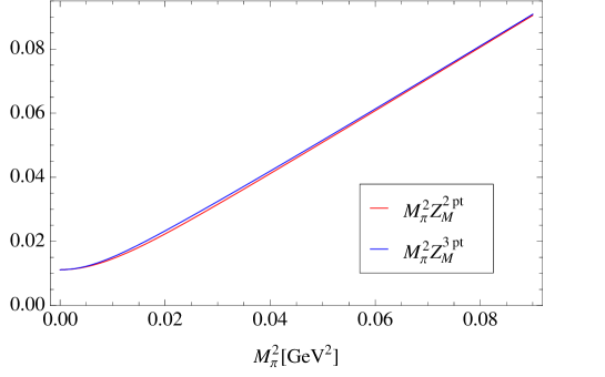
Therefore, these ratios , and should cancel the and dependences, and directly give the values of .
JLQCD collaboration Fukaya:2014jka has employed the latter ratios and found a good plateau for it, extracting a pion charge radius, which is consistent with the experiment.
It should be noted that except for , which is essentially irrelevant in both of the above ratios, we don’t need any zero-mode integrals which could have been a complicated combination of Bessel functions. The remaining finite volume effect in is a perturbative correction from the non-zero modes only and thus, is expected to be small as shown in the next subsection.
V.2 Remaining Finite Volume Effects from non-zero modes
After removing the dominant finite volume effect from the zero-mode, what remains in is the effect of the non-zero momentum modes, which is expected to be perturbatively small. In this subsection, we compute this non-zero-momentum effect to the pion 1-loop and numerically confirm this expectation.
To this end, all we need to evaluate is
| (103) |
Here and in the following, we ignore the terms proportional to , since they are always contracted with a perpendicular 4-momentum vector to , and thus do not contribute to the final result.
It is not difficult to decompose it as
| (104) |
where
| (105) |
Note that is the infinite volume limit of and thus, the finite volume correction is given by
| (106) |
In the standard manner, each contribution can be computed as
where , and denotes the -th modified Bessel function. Here, we have neglected a term proportional to , since that term is proportional to after the summation over .
When , it is straight forward to numerically evaluate the above form. However, when , we need a special care because we need to analytically continuate the results with respect to . Here we simplify the situation using an inequality
| (108) |
in Eq. (V.2). Namely we neglect the oscillating factor . Then the analytic continuation of has no subtlety since the Bessel functions are all vanishing in the limit with any complex phase. Note here that the real part is always positive. We do not think this over-estimation affects the result very much, since the temporal direction is usually larger than the spacial direction by a factor of 2 or 3, and therefore, the contribution from is much smaller from the beginning.
Taking direction the finite volume correction to can be computed as
| (109) | |||||
where
| (110) |
Note that .
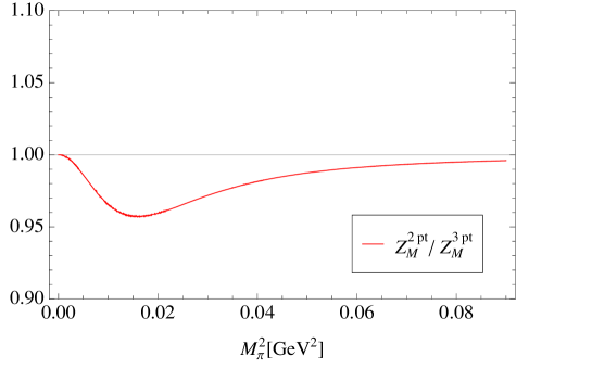
Our numerical estimates for at are presented in Fig. 2. Here, we denote , assuming the dispersion relation of the pion energy, , and choose , , as inputs. The zig-zag behavior may be due to the lack of the rotational symmetry on the lattice. Since is an quantity, our result shows the remaining finite volume effects is around a few % already at , even when .

VI Summary and discussion
We have studied finite volume effects on the electro-magnetic pion form factor in the regime. The pseudoscalar-vector-pseudoscalar three point function has been calculated in the expansion of chiral perturbation theory to the next-to-leading order.
The dominant finite volume effects, which come from the zero-mode of the pions can be removed by two simple manipulations: by inserting non-zero momentum to relevant operators (or making a subtraction at different time correlators) and taking a appropriate ratio of them. After these manipulations, one can safely extract the electro-magnetic pion form factor for which the remaining finite volume correction from the non-zero modes is suppressed to a few percent level already at even in the regime (see Figure 2).
It is important to note that our analysis has been done without using any special features of the expansion, and the dominance of the zero-mode contribution is expected to be a common feature of finite volume effects in any regime of QCD. Therefore, our method can be useful for simulations in the regime, including the ones with twisted boundary conditions Mehen:2005fw ; Tiburzi:2014yra . We also expect a wide application to other quantities like form factors of heavier hadrons.
The authors thanks P. H. Damgaard, S. Hashimoto, T. Onogi, S. Yamaguchi for useful discussions. The work of HF is supported by the Grant-in-Aid of the Japanese Ministry of Education (No. 25800147).
References
- (1) J. Gasser and H. Leutwyler, Annals Phys. 158, 142 (1984);
- (2) J. Gasser and H. Leutwyler, Nucl. Phys. B 250, 465 (1985).
- (3) B. B. Brandt, Int. J. Mod. Phys. E 22, 1330030 (2013) [arXiv:1310.6389 [hep-lat]].
- (4) J. Koponen et al., arXiv:1311.3513 [hep-lat].
- (5) H. Fukaya et al., (JLQCD Collaboration), arXiv:1211.0743 [hep-lat].
- (6) H. Fukaya, S. Aoki, S. Hashimoto, T. Kaneko, H. Matsufuru and J. Noaki, Phys. Rev. D 90, 034506 (2014) [arXiv:1405.4077 [hep-lat]].
- (7) M. Kieburg, J. J. M. Verbaarschot and S. Zafeiropoulos, Phys. Rev. D 88, 094502 (2013) [arXiv:1307.7251 [hep-lat]].
- (8) S. Aoki et al., arXiv:1310.8555 [hep-lat].
- (9) J. Gasser and H. Leutwyler, Phys. Lett. B 184, 83 (1987).
- (10) H. Fukaya and T. Suzuki, arXiv:1402.2722 [hep-lat].
- (11) F. C. Hansen, Nucl. Phys. B 345, 685 (1990).
- (12) F. C. Hansen and H. Leutwyler, Nucl. Phys. B 350, 201 (1991).
- (13) P. Hernandez and M. Laine, JHEP 0301, 063 (2003) [hep-lat/0212014].
- (14) L. Giusti, P. Hernandez, M. Laine, P. Weisz and H. Wittig, JHEP 0411, 016 (2004) [hep-lat/0407007].
- (15) F. Bernardoni, P. H. Damgaard, H. Fukaya and P. Hernandez, JHEP 0810, 008 (2008) [arXiv:0808.1986 [hep-lat]].
- (16) P. Hernandez, M. Laine, C. Pena, E. Torro, J. Wennekers and H. Wittig, JHEP 0805, 043 (2008) [arXiv:0802.3591 [hep-lat]].
- (17) S. Aoki and H. Fukaya, Phys. Rev. D 84, 014501 (2011) [arXiv:1105.1606 [hep-lat]].
- (18) H. Leutwyler and A. V. Smilga, Phys. Rev. D 46, 5607 (1992).
- (19) K. Splittorff and J. J. M. Verbaarschot, Phys. Rev. Lett. 90, 041601 (2003).
- (20) Y. V. Fyodorov and G. Akemann, JETP Lett. 77, 438 (2003).
- (21) S. Aoki et al. [JLQCD and TWQCD Collaboration], Phys. Rev. D 80, 034508 (2009).
- (22) T. Kaneko et al.[JLQCD Collaboration], PoS LATTICE2010, 146 (2010).
- (23) F. Bernardoni and P. Hernandez, JHEP 0710, 033 (2007) [arXiv:0707.3887 [hep-lat]].
- (24) S. Aoki and H. Fukaya, Phys. Rev. D 81, 034022 (2010) [arXiv:0906.4852 [hep-lat]].
- (25) C. Bernard [MILC Collaboration], Phys. Rev. D 65, 054031 (2002) [arXiv:hep-lat/0111051].
- (26) P. Hasenfratz and H. Leutwyler, Nucl. Phys. B 343, 241 (1990).
- (27) P. H. Damgaard and H. Fukaya, Nucl. Phys. B 793, 160 (2008) [arXiv:0707.3740 [hep-lat]].
- (28) T. Mehen and B. C. Tiburzi, Phys. Rev. D 72, 014501 (2005) [hep-lat/0505014].
- (29) B. C. Tiburzi, arXiv:1407.4059 [hep-lat].
Appendix A Zero-mode integral
In this appendix, we evaluate the integrals which are necessary for numerical estimation of or . Although our analysis in this paper is done only in the unquenched QCD, we use the partially quenched results by Splittorff-Verbaarschot ; Fyodorov-Akemann , because some expressions are simpler for the partially quenched results, and the results would be easily extended to the partially quenched study in these expressions. The unquenched results are obtained simply by setting the valence quark mass to the one of the sea quark masses.
We start with the so-called graded partition function which consists of bosons and fermions. Its non-perturbative analytic form is given by Splittorff-Verbaarschot ; Fyodorov-Akemann
| (111) |
in a fixed topological sector of . Here ’s are defined as for and for , where and are the modified Bessel functions. Partial quenching is completed by taking the boson masses to those of valence fermions.
Integrals of some diagonal matrix elements are obtained by simply differentiating the partition function,
| (112) | |||||
and
| (113) | |||||
Then, integrals for the degenerate case can be written as
| (114) | |||||
| (115) | |||||
| (116) | |||||
| (117) | |||||
| (118) | |||||
| (119) |
| (120) | |||||
| (121) |
Here, we have used
| (122) |
Note that the derivative is taken w.r.t the valence degree of freedom after limit is taken. This partially quenched expression is simpler than that of unquenched theory, as shown in Ref. Damgaard:2007ep .
It is also useful to note
| (123) |
which was shown in Appendix of Ref Aoki:2011pza . With this, the following non-trivial relations are obtained,
| (124) |
Similarly, we can use
| (125) |
Appendix B Loop momentum summations
In the calculation of the one-loop diagram, we have encountered the momentum summation:
| (126) |
From the symmetry, on a finite volume we can decompose it as
| (127) |
Note that another possible choice is not independent from the others since .
For a vector which satisfy we can simplify
| (128) |
In particular, it is useful to note
| (129) |
where
| (130) |