Revisiting the method of characteristics via a convex hull algorithm
Abstract
We revisit the method of characteristics for shock wave solutions to nonlinear hyperbolic problems and we describe a novel numerical algorithm —the convex hull algorithm (CHA)— in order to compute, both, entropy dissipative solutions (satisfying all relevant entropy inequalities) and entropy conservative (or multivalued) solutions to nonlinear hyperbolic conservation laws. Our method also applies to Hamilton-Jacobi equations and other problems endowed with a method of characteristics. From the multivalued solutions determined by the method of characteristic, our algorithm ”extracts” the entropy dissipative solutions, even after the formation of shocks. It applies to, both, convex or non-convex flux/Hamiltonians. We demonstrate the relevance of the proposed approach with a variety of numerical tests including a problem from fluid dynamics.
keywords:
hyperbolic equations , method of characteristics , numerical algorithm , compressible fluidMSC:
[2010] 76L05 , 65L05 , 35L60 , 35L03 August 20141 Introduction
The so-called ‘method of characteristics’ allows one to determine smooth solutions to nonlinear hyperbolic equations. The solution formula takes the form and is uniquely determined by the prescribed initial data of the Cauchy problem under consideration and, on the other hand, the family of characteristics associated with the problem. (Here, denotes a parametrization associated with the initial data.) For nonlinear equations, this method generally fails for large times —due to the formation of shock waves. In the present paper, we demonstrate that the characteristics are still of interest beyond the formation of shocks, provided the method is suitably reformulated.
-
1.
In our setting, it is natural to distinguish between two notions of solutions:
- (a)
-
(b)
The entropy conservative solutions, which satisfy entropy equalities and are ”highly oscillating” (and represent the multivalued solutions ForestierLeFloch .
-
2.
We exhibit here two novel formulas (see (3.5) and (3.6)), which rely on a convex hull construction. Importantly, these formulas provide us with a numerical algorithm which is presented and implemented in the present paper. It is found to efficiently compute weak solutions with shocks for both convex and non-convex flux-functions.
We present our method in the context of multi-dimensional problems for, both, nonlinear hyperbolic conservation laws and Hamilton-Jacobi equations. We discuss several important properties of the solutions and perform numerical experiments. In particular, we demonstrate numerically that we recover the entropy solutions. The present paper is concerned with the numerical aspects of our approach, while a follow-up work will provide theoretical support for our new formulation. We also emphasize that the proposed method in principle should apply to a wide variety of nonlinear problems, provided they admit a method of characteristics. We apply it here to convex and non-convex conservation laws and to a problem of fluid dynamics. We expect our method to be applicable to other hyperbolic problems.
We work in a spatial domain which is taken to be throughout this paper. We consider functions defined for positive times and satisfying one of the following two Cauchy problems:
-
1.
Nonlinear conservation laws:
(1.1) where is a given flux-function and denotes the divergence .
-
2.
Hamilton-Jacobi equations:
with a given Hamiltonian , where denotes the gradient. In fact, by introducing the unknown , we can equivalently consider the following system of nonlinear hyperbolic equations:
(1.2)
Clearly, the constraint , i.e. the fact that is a gradient, is satisfied for all times provided it holds at the initial time.
The method of characteristics applies to both problems and generates a smooth solution for sufficiently small times (at least) in the following form (cf. the notation below):
| (1.3) |
where the map parametrizes the family of characteristics. Our main observation based on the novel notion of convex hull transform allows us to generalize the characteristic method to all times, by relying on two explicit formulas (cf. (3.5) and (3.6)). Since the characteristic map is onto, defining its inverse requires some care, and this issue is addressed below.
Since our formulas are based on a reformulation of the characteristic method, the approach we propose here is very general and should apply to many nonlinear hyperbolic problems. At the end of this paper, we for instance discuss an application to fluid dynamics. Our formulas are easily implemented in numerical applications (cf. the discussion in Section 4 below) and allows us to compute solutions for all times and for all dimensions . The method applies to arbitrary equations like (1.1) and (1.2), including non-convex flux-functions and non-convex Hamiltonians.
In term of efficiency, our algorithm can favorably compete with spectral techniques such as the ones proposed for nonlinear hyperbolic problems by Sidilkover and Karniadakis SK and followers, as well as techniques where the Rankine-Hugoniot relations are directly enforced at the discrete level such as the one proposed by Jaisankar and Raghurama Rao JR . Importantly, we expect the proposed method to generalize to many problems which admits a classical method of characteristics; for instance, problems with source-terms. Our approach could provide a robust alternative (or supplementary tool) to design well-balanced techniques, such the ones in Boscarino and Russo BoscarinoRusso .
2 The convex hull transformation
2.1 Motivation
The present subsection provides a motivation for the present paper, but the reader unfamiliar with measure theory can skip this subsection and read directly the next subsection. Without genuine loss of generality, we will work with smooth and spatially decaying initial data (so that the derivatives are integrable). Let be a convex set with unit Lebesgue measure and, typically, we can work with the unit cube . By unit measure, we mean that , where stands for the Lebesgue measure. More generally, we use the notation for the measure of a set with respect to a finite measure .
Let us first consider general maps , defined on an open, bounded, and convex set (with ) and taking values in a convex and open set . As usual, we denote by the set of all positive measures on with unit total mass. Given two probability measures and , we say that a map is –measure preserving (or transports into ) if and only if , that is, for all (-measurable) sets . This condition is equivalent to the change of variable formula .
According to the general theory of optimal transport, given and for a positive probability measure satisfying and (that is, is absolutely continuous with respect to the Lebesgue measure), these exists a unique map ”transporting” the Lebesgue measure on into . More precisely, let be a square-integrable map and consider the probability measure . Then the following decomposition
| (2.1) |
holds and is called the polar factorization of the map . Here, by definition, the map is thus Lebesgue-measure preserving.
The following remark in also in order: the convex factorization is known to be unique when the measure is absolutely continuous with respect to the Lebesgue measure, but uniqueness might be lost otherwise. In the present paper, due to the presence of shock waves, this uniqueness will not necessary hold.
2.2 A novel notion
Let be a square-integrable and surjective map of the form . Then, the convex hull transformation of is defined as
| (2.2) |
In view of this definition, is also surjective and the probability measure is in general singular, i.e. need not absolutely continuous with respect to the Lebesgue measure on and may typically contain Dirac masses. In this context, we have the following proposition which allows us to inverse the map by solving the equation when is a prescribed smooth function fixed throughout.
Solving the equation
Monotone maps admit generalized inverses defined as follows. Let be a surjective map and consider the measure . Suppose , where is convex. Given an integrable function defined on , we can introduce the integrable function as the density of the measure with respect to . This function is defined almost everywhere and satisfies for every set
| (2.3) |
We omit here the discussion of the relevant regularity and functional spaces. With the convex hull transformation , the function defined as above, satisfies (by Jenssen inequality)
| (2.4) |
and, by definition, we then say that the convex hull transformation is entropy dissipative.
3 Entropy dissipative/conservative solutions
3.1 The characteristic map
Parametrization of the initial data
We begin by formulating the standard characteristic method, which can be used to compute solutions for sufficiently small times. This holds for both equations (1.1) and (1.2). Observe that our formulation is based on a specific parametrization of the initial data.
We consider either scalar-valued functions or vector-valued maps . As stated in the introduction, the gradient operator is denoted by , while the divergence operator is denoted by ). We introduce the norm for any (piecewise smooth, say) function defined on . If is vector-valued, we write . With this notation, we are given a smooth initial data and we suppose so that does not have “flat part”. This is not a genuine restriction and can be ensured by an arbitrary perturbation of . We then introduce the initial map
| (3.1) | ||||
We observe that is more regular (by one additional derivative) than the function , which itself is solely continuous (with bounded derivatives).
Nonlinear conservation laws
For each time , we define the characteristic map for the conservation law (1.1) as :
| (3.2) |
which admits bounded derivatives up to first order at least.
Hamilton-Jacobi equation
3.2 A novel method of characteristics
We now introduce two explicit formulas, which provide solutions to (1.1) and to (1.2) for all positive times, i.e. beyond shock formation. Consider the characteristic maps for the conservation law and Hamilton-Jacobi equations defined in (3.2)-(3.3), suppose without restriction that is square-integrable.
Entropy conservative
Consider the polar factorization of , see (2.1), with convex and Lebesgue measure preserving. For all positive times, we define the entropy conservative solution as
| (3.5) |
for all positive times, in which the inverse is well-defined since is convex and is measure-preserving.
Entropy dissipative
Suppose , with and consider its convex hull transform , given earlier. We define the entropy dissipative solution
| (3.6) |
for all positive times, in which the generalized inverse was defined earlier. Furthermore, in the general situation , we can introduce a more general transformation of the form , with a (possibly non-trivial) measure-preserving map , but this is unnecessary for our purpose in the present paper.
3.3 Properties of entropy dissipative solutions
We now state some properties of the entropy dissipative solutions. Consider the map and the function defined by the formula (3.6).
-
1.
is continuous and surjective. For almost all , there exists a unique such that
(3.7) -
2.
The function is a weak solution to the conservation law (1.1).
-
3.
At every point of discontinuity of (with limits denoted by ), the map satisfies the Rankine-Hugoniot relations , while, at points of continuity, we can write (in the support ).
-
4.
The entropy condition holds: for instance in one space dimension and at a point of discontinuity where one has for all .
-
5.
In one space dimension and for a convex flux-function, we can recover the Hopf-Lax formula: (3.6) coincides with the following formula with , where is the Legendre-Fenchel transform of the flux.
We recall that the Hopf-Lax formula allows one to compute solutions to (one-dimensional) conservation laws and (multi-dimensional) Hamilton-Jacobi equations when the flux or the Hamiltonian are convex.
4 An illustration with Burgers equation
Before we present our algorithm in full details (in the forthcoming section), we want first to illustrate our formula with a typical example. We thus consider the formulas (3.6)-(3.5) for the inviscid Burgers equation, that is, the equation (1.1) with quadratic flux-function:
| (4.1) |
Here, we define the map by
| (4.2) |
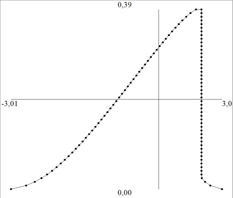
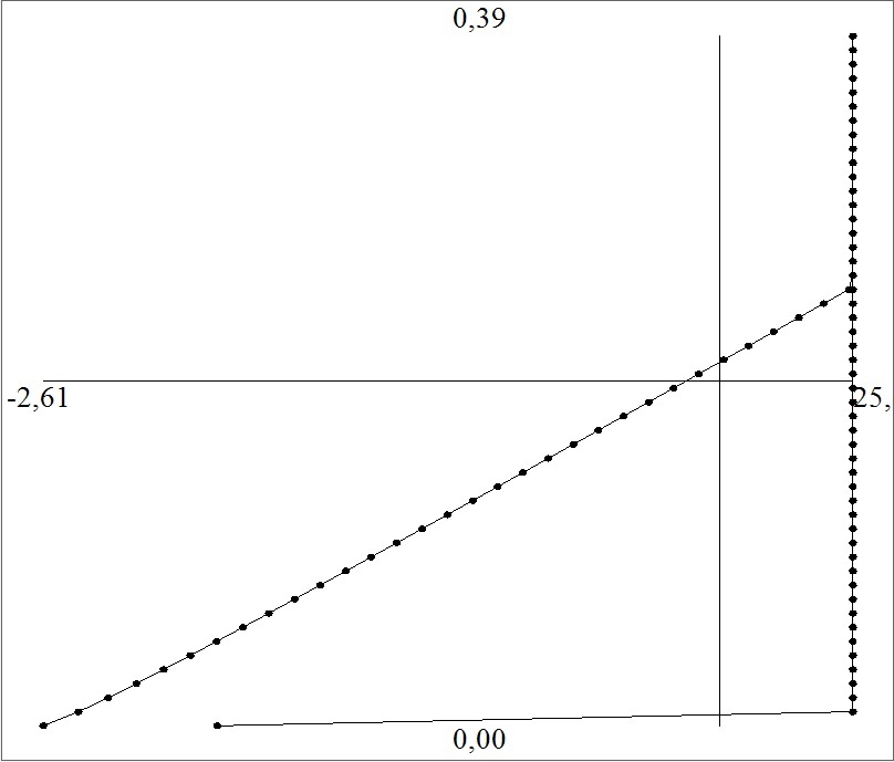
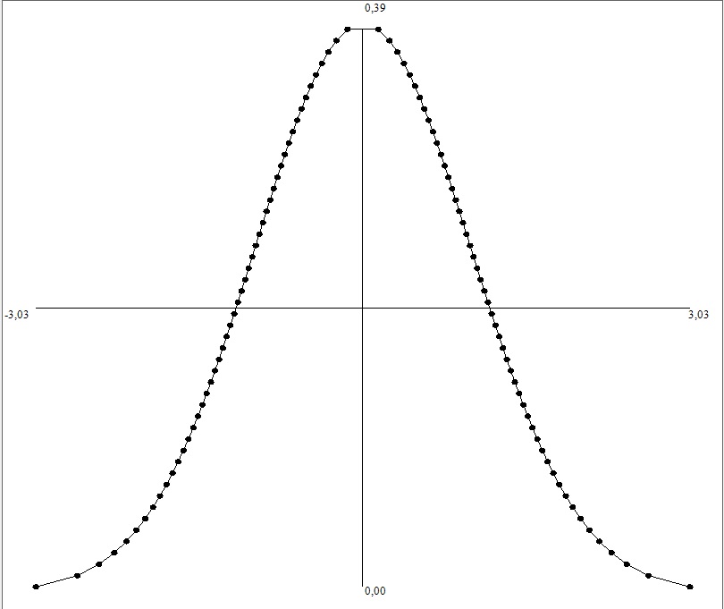
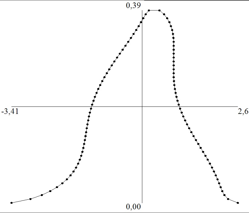
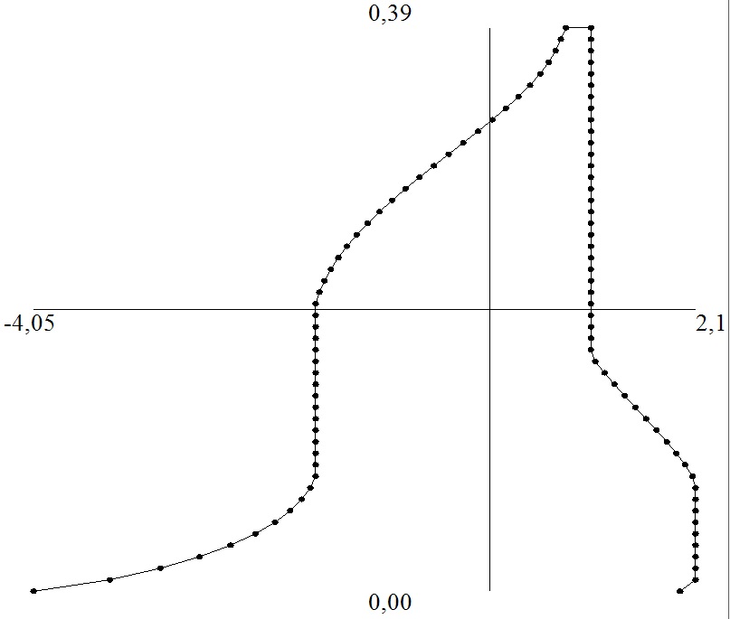
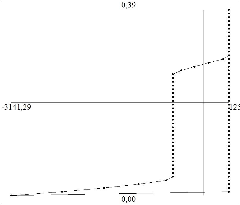
Our numerical results in Figure 4.1 plots the solution computed using the formula (3.6) with the Gaussian initial data
| (4.3) |
As will be explained in the following section, the solution is represented by a cloud of points , with . The simulation is ran with .
 (a) t=0: initial condition
 (b) t=3: smooth regime
|
 (c)t=6: shock formation
 (d) t=106: N-wave regime.
|
Figure 4.1 (a) represents the initial Gaussian condition. Figure 4.1 (b) shows the solution during the smooth regime of evolution. Next, Figure 4.1 (c) displays the solution after the shock formation. Finally, Figure 4.1 (d) (at time ) demontrates the convergence of the solution toward the so-called N-wave, as expected, which is the asymptotic profile solution (up to a translation and to a jump). Observe the formation of a ”spike” in the shock, which is clearly visible at the time . Namely, our method generates an additional spike within the jump discontinuity (which could be easily filtered and removed, if one wishes). Note also the isolated point in Figure 4.1 (d), which is a minor numerical artifact.
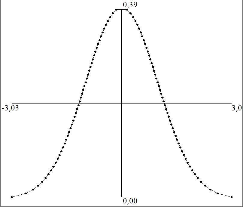
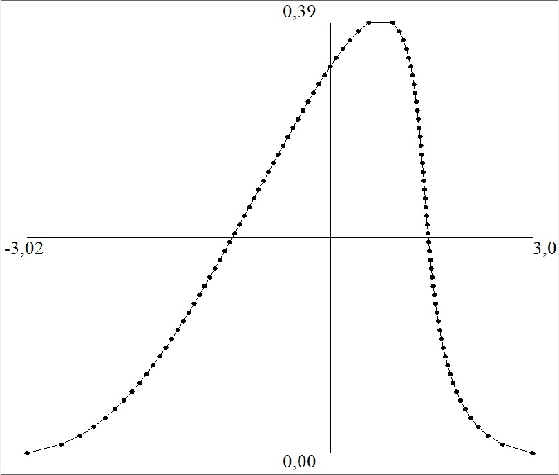
In contrast, Figure 4.2 represents the conservative solution with the same initial condition, but computed with our formula (3.5). We can easily deduce this solution from the multivalued one. The solution is selected among all possible values by using the re-ordering map in the polar factorization (2.1).
 (a) t=0: initial condition
 (b) t=3: smooth regime
|
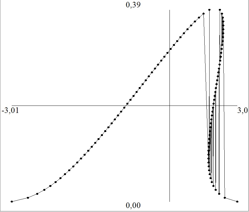 (c) t=6: oscillating regime
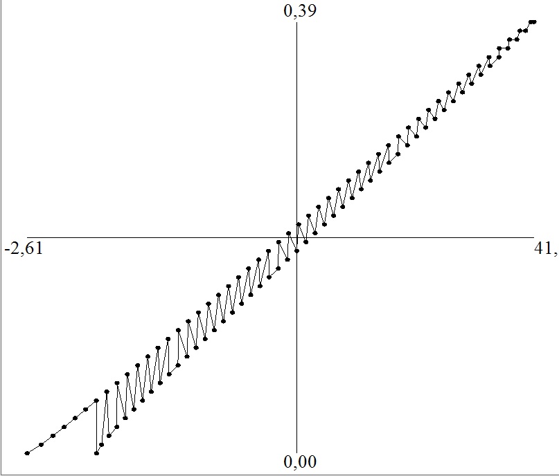 (d) t=106: long time behavior
|
5 Implementation of the convex hull algorithm (CHA)
We now present our algorithm for one-dimensional conservation laws of the form (1.1), that is,
| (5.1) |
We rely on our formulas (3.6) and (3.5), proposed in the first part of this paper. We introduce the map by
| (5.2) |
We are going to our numerical algorithm, step by step, by focusing on Burgers equation, for simplicity in the presentation. The proposed algorithm yields the solution (3.6) or (3.4), and works equally well in any spatial dimension and and with Hamilton-Jacobi equations. We point out that the code based on our method is available Mercier , so that our results can be easily reproduced by the reader. This algorithm will be tested with more complex case studies in the following section.
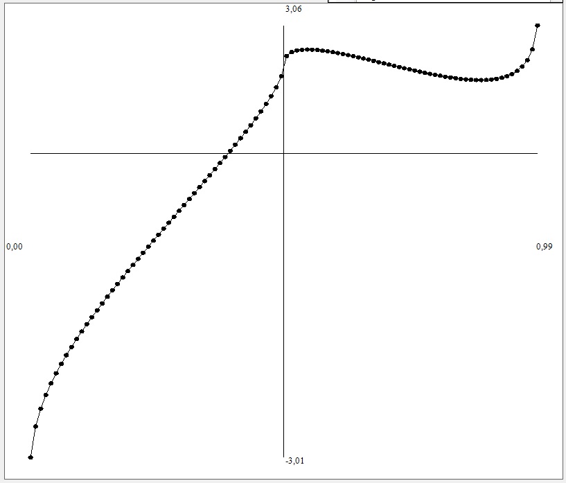
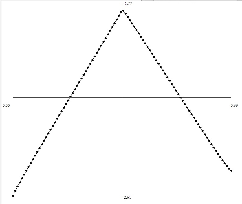
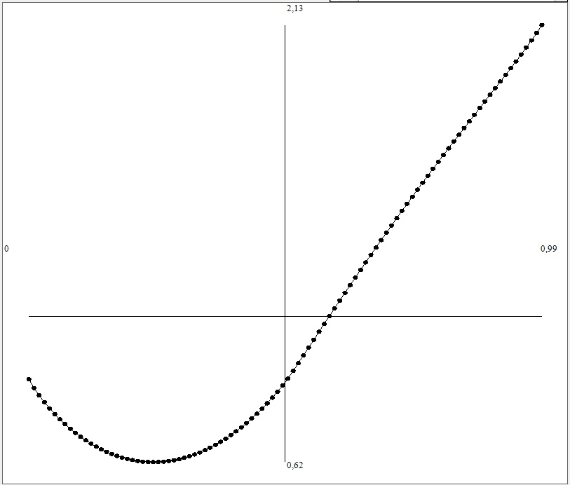
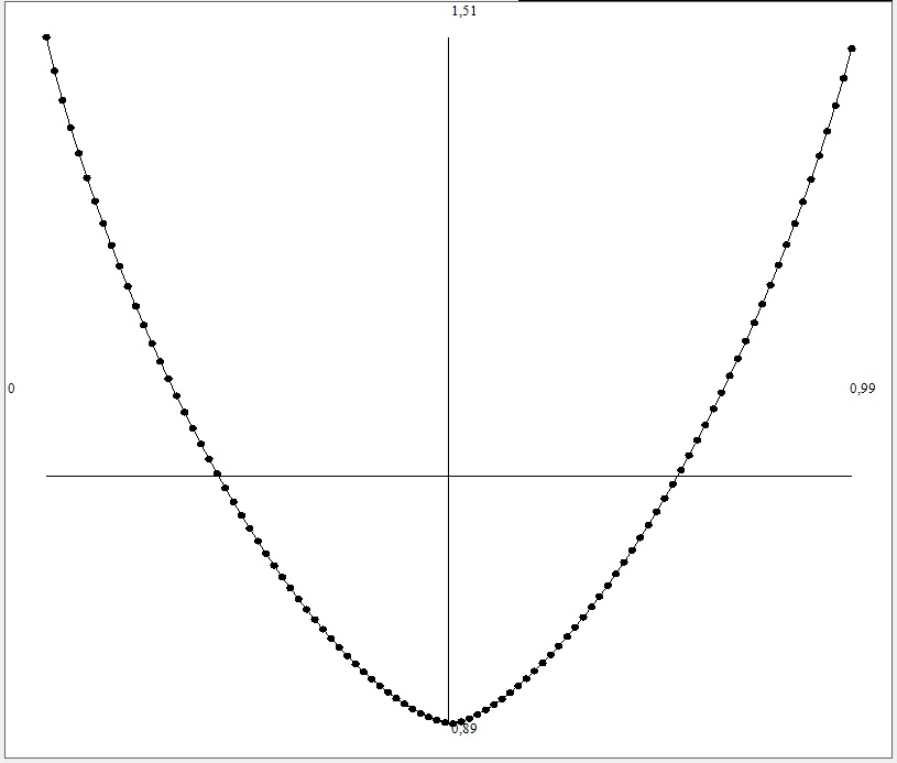
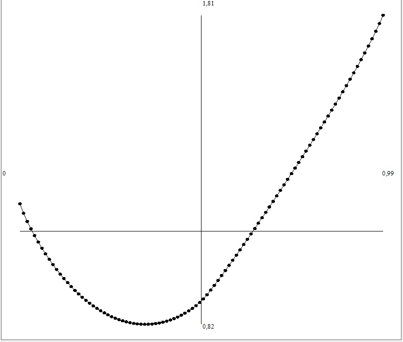
We focus on the formula (3.6) and on Burgers equation studied in the previous section. Our construction is as follows: we consider the characteristic map , where and we set . For the numerical tests, we will always use (with in this paper) and . Our Convex Hull Algorithm (CHA) amounts to determine the solution
| (5.3) |
in which
| (5.4) |
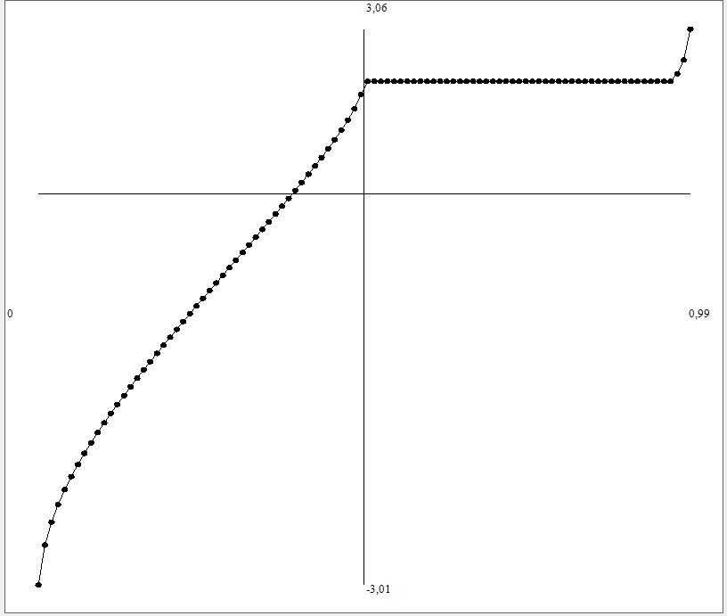
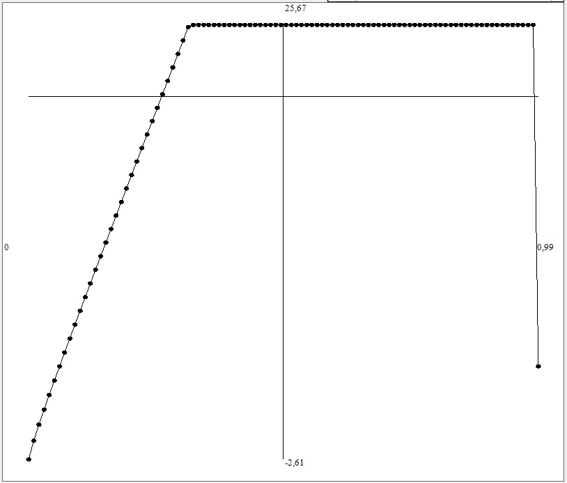
The main steps of this algorithm are as follows, for each time :
-
1.
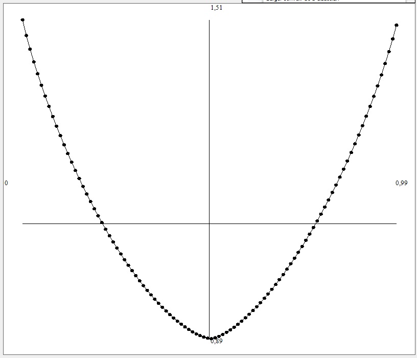
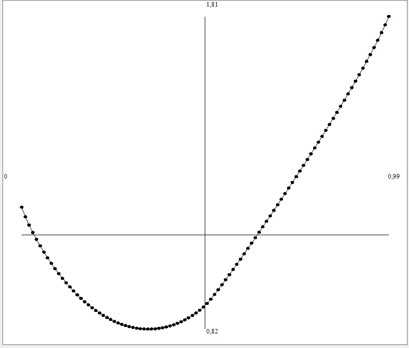
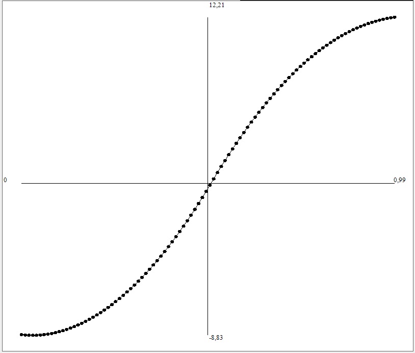
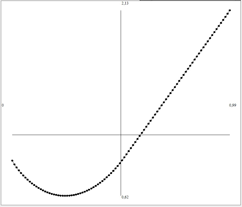
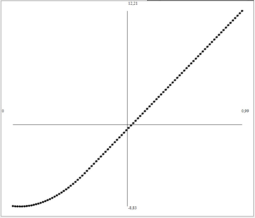
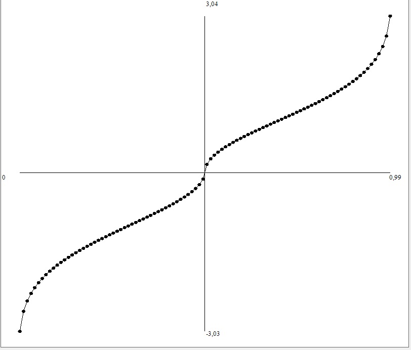
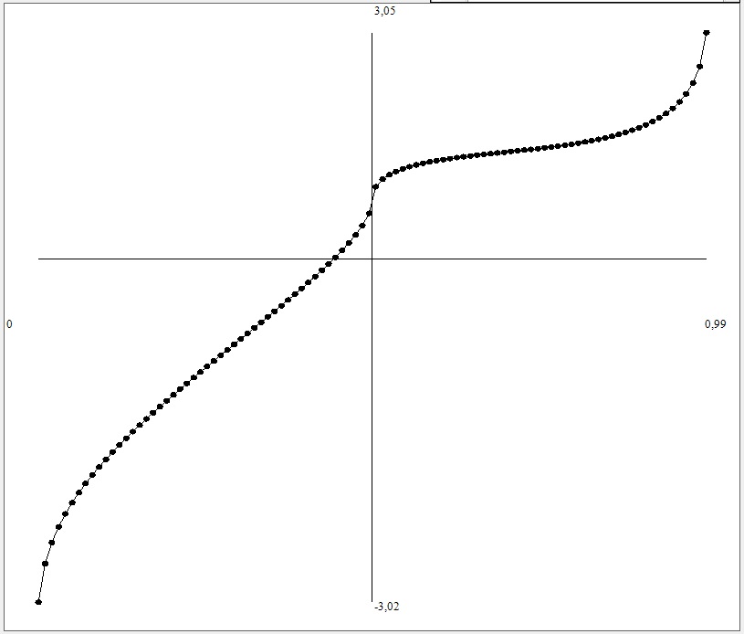
Step 1. Compute the characteristic map (as illustrated by Figure 5.1) and its companion function (see Figure 5.2), deduced coming from of a Helmholtz-Hodge decomposition of the form
(5.5) where the map is a divergence-free, i.e. . In one space dimension, we can always normalize to vanish identically.
-
2.
Step 2. Compute the convex hull of the function . This step is illustrated by Figure 5.3.
- 3.
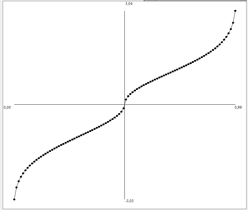 (a) t=0
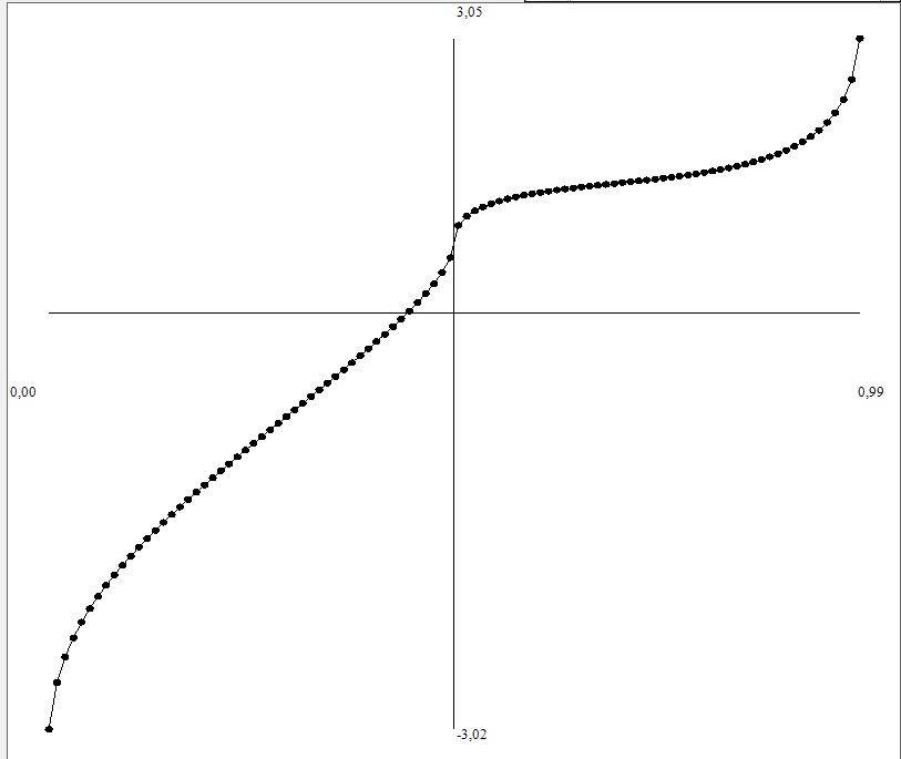 (b) t=3
|
 (c) t=6
 (d) t=106
|
 (a) t=0
 (b) t=3
|
 (c) t=6
 (d) t=106
|
 (a) t=0
 (b) t=3
|
 (c) t=6
 (d) t=106
|
 (a) t=0
 (b) t=3
|
 (c) t=6
 (d) t=106
|
Concerning Step 2, efficient algorithms in order to compute convex hulls are available as open source softwares. (See, for instance, http://www.cgal.org.) We used the specialized QHull library available at http://www.qhull.org. Our numerical contribution for the present work is a Helmoltz-Hodge decomposition/re-composition code based on multi-dimensional unstructured meshes, which can be described as follows.
Let us introduce the following non-local basis functions , where :
| (5.6) |
Let , be distincts sampling points of the computational domain , with in our one-dimensional setting. We then consider any (possibly) vector-valued map and the following minimization problem
| (5.7) |
which can be interpreted as a classical projection method. This latter problem is approximated by a linear system corresponding to a Gram-Schmidt algorithm (in which the notation is used for the integral of the scalar product of two vector-valued functions):
| (5.8) | ||||
This linear system is invertible, provided , and the right-hand side approximation makes sense for all maps that are finite sums of convex and concave functions. Once the coefficients are computed, the component is obtained by
| (5.9) |
Once the convex hull is computed, a similar algorithm yields us the components of the projection . This allows us to finally compute
| (5.10) |
6 Applications
6.1 A fluid dynamical problem
Finally, we consider the coupling between Burgers equation satisfied by the velocity function , that is,
| (6.1) |
and a linear transport equation for a passive scalar (cf. LeFloch90 for a mathematical background):
| (6.2) |
By setting , we can interpret as solutions to the system of fluid dynamics
| (6.3) |
| (6.4) |
Let be the characteristic map for Burgers equation, i.e. . Consider the function
| (6.5) |
with which we can compute (at least formally) Hence, , provided is surjective, so that (6.3)-(6.4) is satisfied. Consequently, we obtain the function associated with the density .
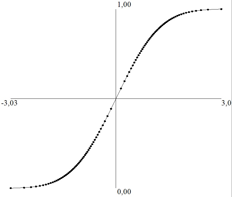
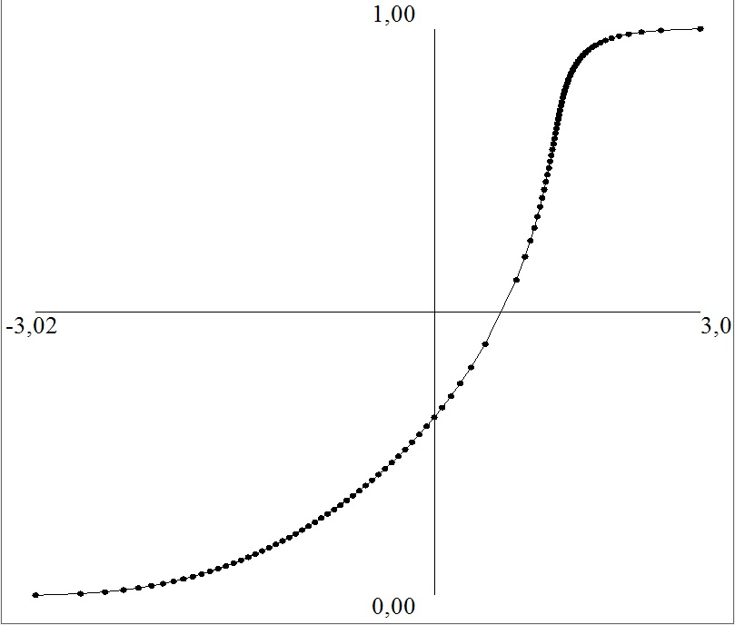
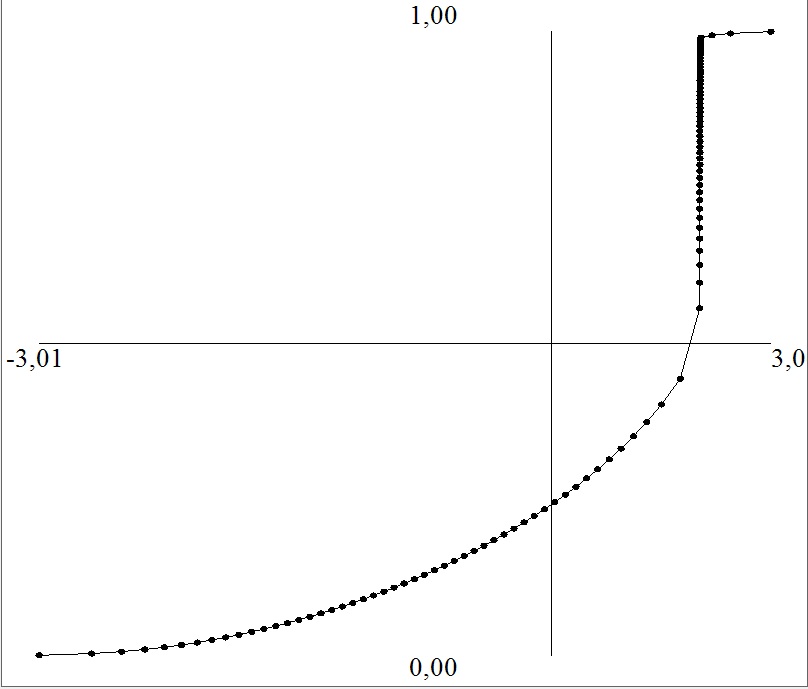
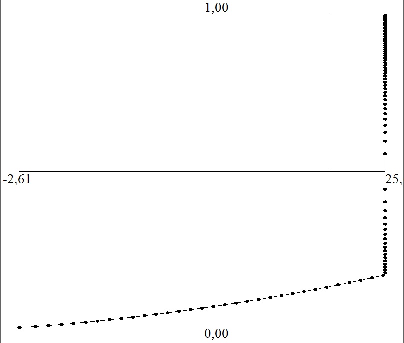
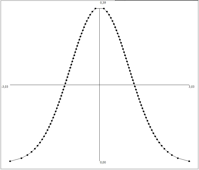
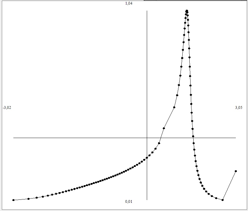
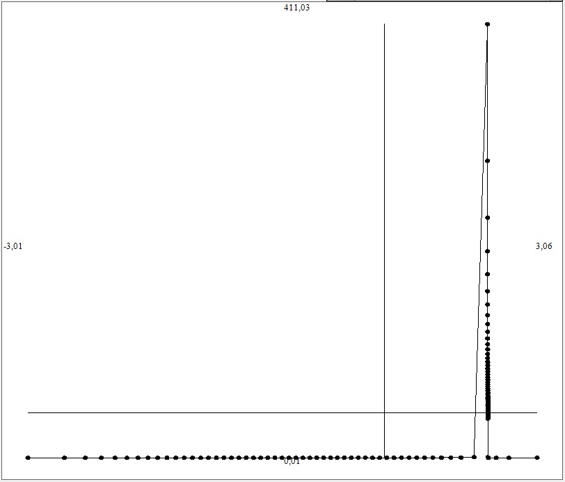
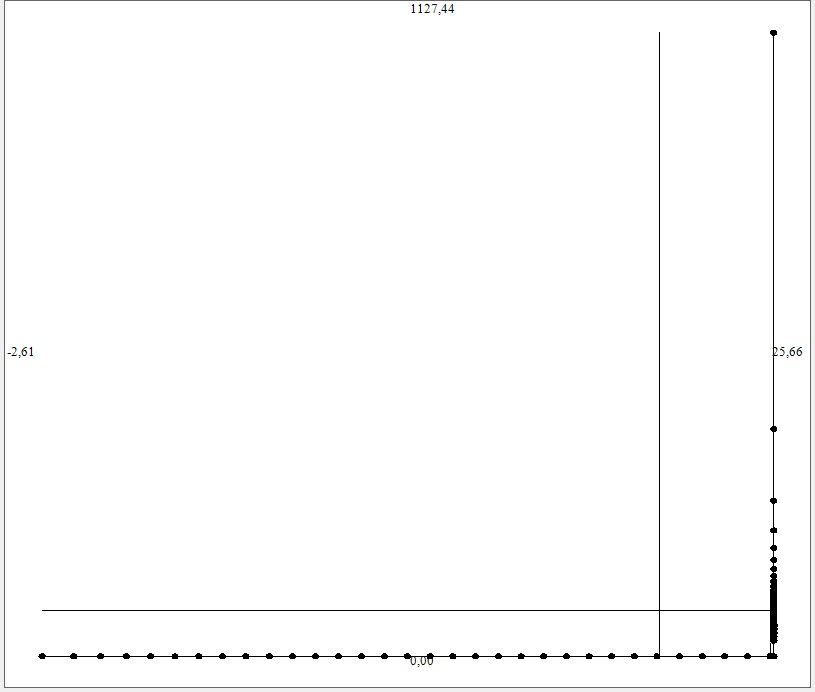
Figures 6.1 and 6.2 display the results of our numerical method for this problem. We have plot both and , where the initial density is taken as
| (6.6) |
The velocity follows Burgers equation, and is computed as we explained earlier. (See Figure 4.1 for the velocity at the corresponding times.) Note that the density is singular after the shock formation, and we thus performed a suitable truncation in order to display the function in Figure 6.2.
 (a) t=0
 (b) t=3
|
 (c) t=6
 (d) t=106
|
 (a) t=0
 (b) t=3
|
 (c) t=6
 (d) t=106
|
6.2 Conservation laws with one inflection point
We next investigate the class of conservation laws of the form (1.1) with non-convex flux. Such laws arise in, for instance, material science or the dynamics complex fluid flows.
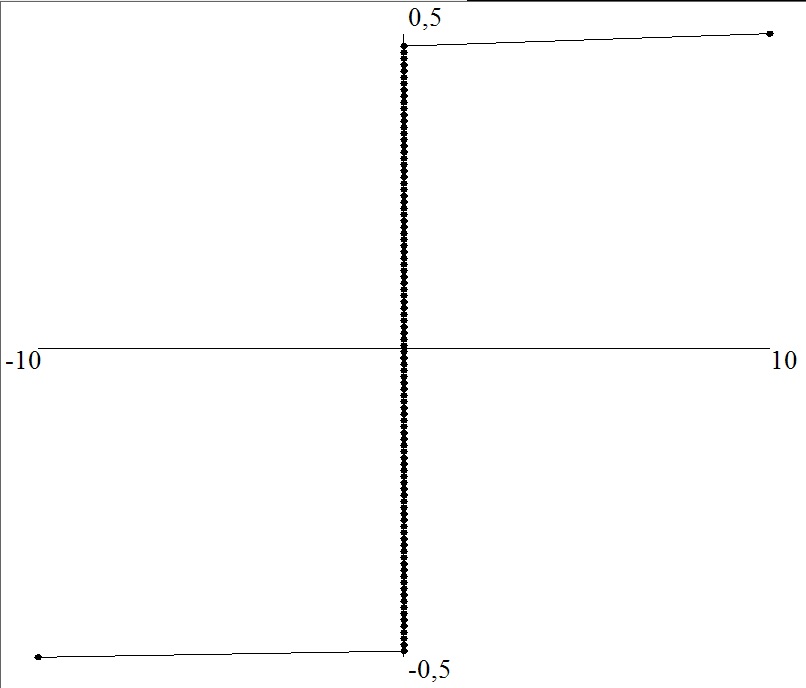
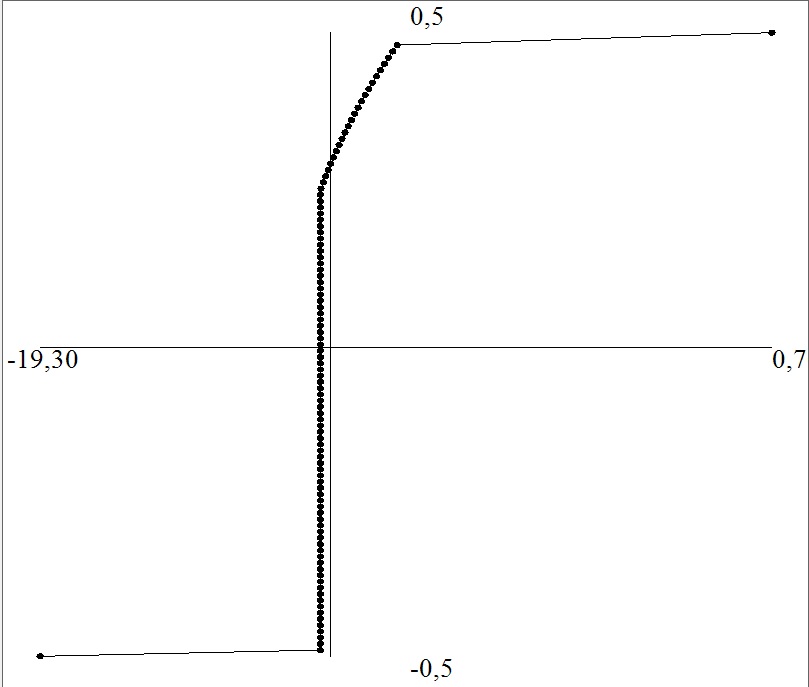
Specifically, in (5.1), we choose . The first numerical test corresponds to Riemann data generating a non-monotone shock formation, that is a shock followed by a rarefaction wave ; see Figure 6.3:
 t=0.
t=0.
 t=10.
t=10.
|
For our second numerical test, we use an initial data with two shocks, which initially separated but interact at a later time. After the interaction, the middle state cancels out and the solution stabilizes to single shock traveling at a negative velocity (cf. Figure 6.4):
It is remarkable that, even for such a non-convex flux, our algorithm generates the entropy solution (i.e. physically meaningful) to the problem, which is the one characterized in Kruzkov .
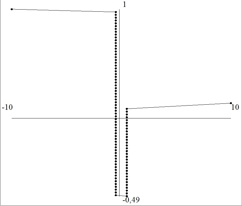 (a) t=0
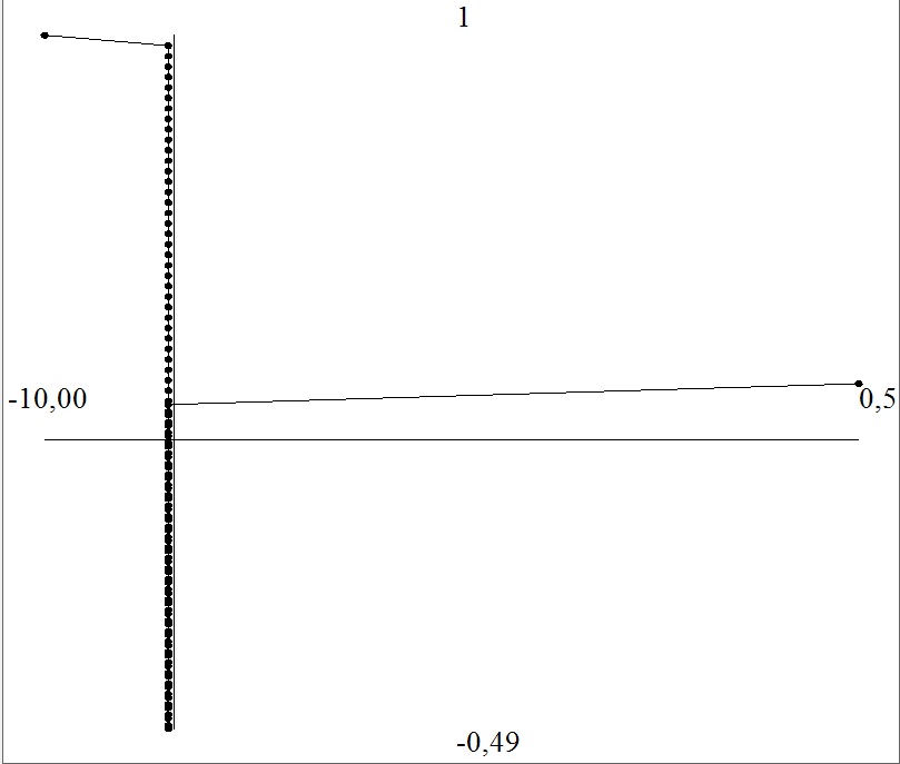 (b) t=10
|
6.3 Conservation laws with several inflection points
We finally apply the CHA method to a conservation law whose flux admits several inflection points. Specifically, we consider the nonconvex function
| (6.7) |
This example provides us with a further challenge for our method. The first test we consider corresponds to the Riemann data
| (6.8) |
with which the solution is expected to exhibit a rather complex wave pattern, that is, two rarefaction waves and two shocks. The numerical results are strikingly in accordance with the theoretically expected ones; see Figure 6.5.
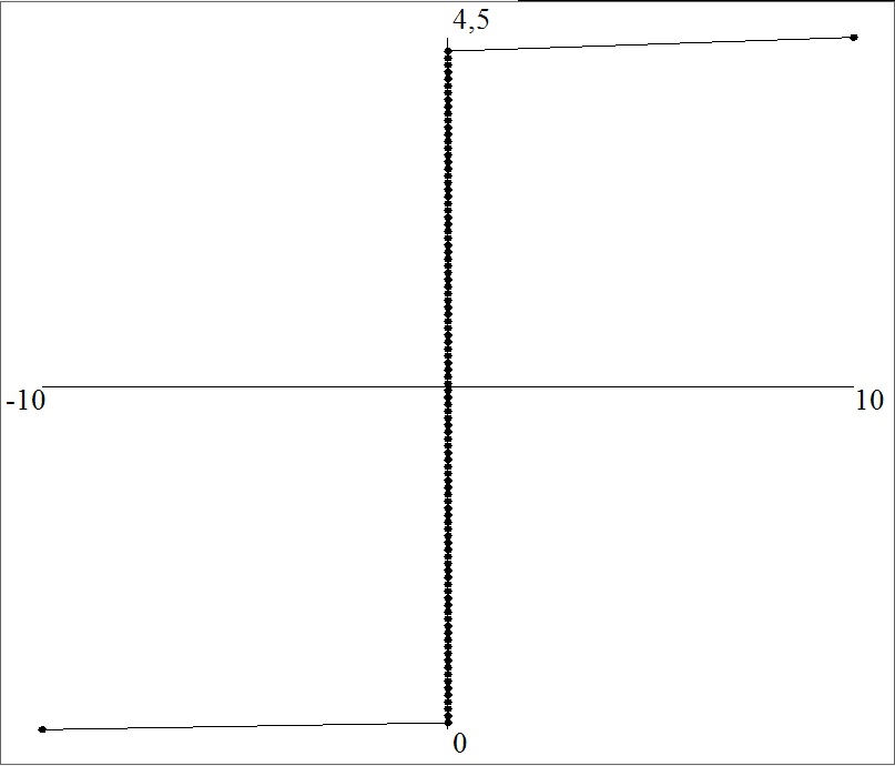 t=0
t=0
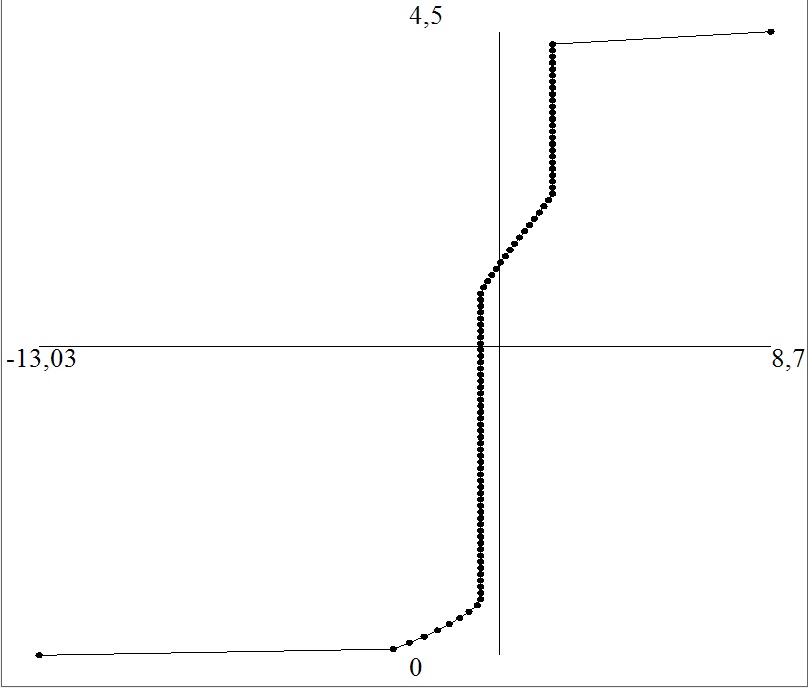 t=20
t=20
|
Second, we investigate the time-asymptotic behavior of the CHA-algorithm with the same flux of degre five, but now with a Gaussian initial data (as defined earlier). Even though this data generates a complex wave pattern for sufficiently small times, the solutions are expected to converge toward a generalization of the N-wave of the convex case. Such a kind of convergence is indeed observed with our method, as illustrated by Figure (6.6). Yet, we emphasize the non-trivial shape of the asymptotic N-wave in this case.
 t=0.
t=0.
 t=.5
t=.5
|
 t=1.
t=1.
 t=1001
|
7 Concluding remarks
The method proposed in this paper has the following advantages:
-
1.
The method applies to hyperbolic problems and Hamilton-Jacobi equations. It generates solutions at any arbitrary time and does not require a time-evolution. In particular, we can easily compute the solutions at an arbitrary large time and therefore determine the asymptotic regime of the solutions (such as the -wave profile for convex hyperbolic equations).
-
2.
The key observation made in this work is that the multivalued solutions contains all the ”information” about the entropy dissipative solutions, so that the latter can be recovered from the former by our convex hull algorithm (CHA).
-
3.
The jump discontinuities in solutions (shock waves) are sharply represented and described with finitely many points proportionally to the discontinuity strength. This is in contrast with methods based on finite difference schemes for which the numerical solutions contain only a few points within the shocks.
-
4.
Especially in a multidimensional setting, the sampling (cf. Section 5) should be chosen to be equidistributed in . Such a set can be computed by a random generator, but a better choice is an optimal quantizer of the ”uniform law”, which can be achieved when the initial condition is written as a discrete sum of convex and concave components.
-
5.
Optimization strategies can be developed for the proposed algorithm. For instance, removing discrete points lying inside the convex hull and adding discretization points outside. Such a strategy allows for instance to keep the discretization error bounded uniformly in time.
Acknowledgments
The first author (PLF) was partially supported by the Centre National de la Recherche Scientifique (CNRS) and the Agence Nationale de la Recherche through the grants ANR 2006–2-134423 and SIMI-1-003-01.
Bibliography
References
- [1] Boscarino S. and Russo G., On a class of uniformly accurate IMEX Runge–Kutta schemes and application to hyperbolic systems with relaxation, SIAM J. Sci. Comput. 31 (2009), 1926–1945.
- [2] Forestier A. and LeFloch P.G., Multivalued solutions to some nonlinear and nonstrictly hyperbolic systems, Japan J. Indus. Appl. Math. 9 (1992), 1–23.
- [3] Hopf E., The partial differential equation , Comm. Pure Appl. Math. 3 (1950), 201–230.
- [4] Jaisankar and Raghurama Rao S.V., A central Rankine-Hugoniot solver for hyperbolic conservation laws, Jour. Comput. Phys. 228 (2009), 770–798.
- [5] Kruzkov S.N., First-order quasilinear equations with several space variables, Math. USSR. Sb. 10 (1970), 217–243.
- [6] Lax P.D., Hyperbolic systems of conservation laws and the mathematical theory of shock waves, CBMS Regional Conference Series in Mathematics No. 11, Philadelphia, SIAM, 1973.
- [7] LeFloch PG., An existence and uniqueness result for two nonstrictly hyperbolic systems, IMA Volumes in Math. and its Appl.,“Nonlinear evolution equations that change type”, ed. B.L. Keyfitz and M. Shearer, Springer Verlag, Vol. 27, 1990, pp. 126–138.
- [8] LeFloch P.G., Graph solutions to nonlinear hyperbolic systems, J. Hyper. Diff. Equa. 1 (2004), 243–289.
- [9] Mercier J.M., A numerical code for nonlinear hyperbolic equations, available at http://www.crimere.com/blog/jean-marc/p=2072.
- [10] Sidilkover D. and Karniadakis G.E., Non-oscillatory spectral element Chebyshev method for shock wave calculations, Jour. Comput. Phys. 107 (1993), 10–22.