NN

See pages 1-last of Mito-PG-MS22ter-CORRb.pdf

SUPPORTING MATERIAL
Interplay of packing and flip-flop in local bilayer deformation. How phosphatidylglycerol could rescue mitochondrial function in a cardiolipin-deficient yeast mutant.

Determination of the pH at the membrane surface

The pH on the GUV membrane during the microinjection of acid solution can be estimated as follows. First, the initial velocity $v_{0}$ of the acid solution when it just flows out of the micropipette into the fluid that surrounds the GUVs, i.e., the velocity right at the tip of the micropipette, is determined from the hydrodynamics inside the micropipette. This initial velocity $v_{0}$ is calculated as a function of the injection pressure, taking into account the geometry of the micropipette. Then, once the acid solution is out of the micropipette, we show that its dynamics is dominated by diffusion, which enables us to calculate the pH in the fluid that surrounds the GUVs, and hence the pH close to the GUV membrane. The diffusion calculation involves the quantity of acid injected per unit time from the micropipette, which acts as a source for the diffusion process. This quantity can be determined from $v_{0}$.

1 Initial velocity $v_{0}$ of the acid solution

In order to estimate the velocity $v_{0}$ of the acid solution at the micropipette tip, we study the hydrodynamics in the micropipette.

Considering that the diameter of the micropipette varies slowly from the point where the injection pressure is imposed to the thin tip of the micropipette, we can approximate the shape of the micropipette as a succession of cylinders where the flow is a standard Poiseuille flow. The pressure drop $P$ in each of these cylinders is related to its diameter $\delta$ through $P\propto\delta^{4}/\ell$, where $\ell$ denotes the length of the cylinder (1). Hence, most of the pressure drop occurs in the thinnest region of the micropipette.

Measurements of the internal diameter of the micropipette tip, performed as described in (2), led to a value of $0.3\,\mu\mathrm{m}$ in our experiments. Moreover, direct observation under the microscope shows that the diameter of the micropipette is approximately constant along the first $\sim 10\,\mu\mathrm{m}$ closest to the tip, beyond which this diameter increases significantly. Hence, almost all the pressure drop occurs in this small cylinder region close to the tip of the micropipette. We thus approximate the velocity $v_{0}$ of the acid solution at the micropipette tip by the average velocity of a Poiseuille flow in a cylinder with diameter $\delta\approx 0.3\,\mu\mathrm{m}$ and length $\ell\approx 10\,\mu\mathrm{m}$ submitted to a pressure drop $P$ equal to the injection pressure, $P\approx 20\,\mathrm{hPa}$. It reads

$$v_{0}=\frac{P\delta^{2}}{32\eta\ell}\,,$$ (1)

which yields $v_{0}\approx 0.56\,\mathrm{mm/s}$ with the above-mentioned values.

In order to check the validity of this approximation, the velocity $v_{0}$ at the tip of the micropipette was also calculated assuming that the small cylinder considered here is followed by a cone and by another cylinder of larger diameter. The order of magnitude of the length and diameter of the cone and of the second cylinder were determined from the microscope observation of the micropipette, and the cone was treated as a succession of infinitesimal cylinders. This calculation yields a value of $v_{0}$ which is smaller than the above value by less than 4%. Thus, the largest source of error in our estimate of $v_{0}$ does not arise from this approximation, but from our limited knowledge of the exact geometry of the tip of the micropipette, and in particular of the effective value of $\ell$, which could vary from one micropipette to another. In order to assess the uncertainty coming from this factor, we used both $\ell=10\,\mu\mathrm{m}$ and $\ell=5\,\mu\mathrm{m}$, and compared the values obtained. The final values of the pH were only marginally affected (see below).

2 Diffusion of the acid solution

Once the acid solution is out of the pipette, its dynamics is determined by diffusion and by Stokes hydrodynamics. The relative importance of these two effects is characterized by the Péclet number $\mathrm{Pe}=vz_{0}/D$, where $v$ is the flow velocity, while $D$ is the diffusion coefficient of hydrochloric acid in water, $D=2/(1/D_{\mathrm{H}^{+}}+1/D_{\mathrm{Cl}^{-}})=3347\,\mu\mathrm{m^{2}/s}$ at infinite dilution and at $20\,^{\circ}\mathrm{C}$ (3), and $z_{0}$ is a characteristic distance of the flow, which is taken as the distance between the membrane and the micropipette tip, i.e., about $10\,\mu\mathrm{m}$. Although the actual characteristic length scale over which the velocity varies is in fact smaller (see below), we take this value in order not to risk underestimating the Péclet number. At the very tip of the micropipette, where $v=v_{0}$, $\mathrm{Pe}\approx 1.7$, which implies that both hydrodynamic flow and diffusion are initially important. However, away from the micropipette, the velocity of the flow decreases, and hence diffusion becomes dominant. To demonstrate this, we first assume the opposite, i.e. that hydrodynamics is dominant over diffusion, thereby overestimating the flow velocity. In this case, the flow corresponds to a Stokes jet (4, 5). Flow conservation (or, equivalently, more complete Stokes jet dynamics, see (4, 5)) entails that at a distance $L$ from the source, the flow velocity is $v\approx v_{0}\delta^{2}/(16L^{2})$. For $L=1\,\mu\mathrm{m}$, we obtain $v\approx 3.2\,\mu\mathrm{m}/s$, which gives a Péclet number $\mathrm{Pe}=vz_{0}/D\approx 10^{-2}$, in contradiction with the initial assumption. This shows that once the acid solution is more than $1\,\mu\mathrm{m}$ away from the micropipette tip, its dynamics is dominated by diffusion. This in line with our previous experimental work (Fig. 6 of Ref. (6)) in which the injection of a fluorescent substance under identical conditions led to the observation of a quasi-spherical fluorescent “cloud” characteristic of diffusion.

Thus, in order to calculate the pH profile in the fluid that surrounds the GUVs, we can consider that the acid solution simply diffuses from the micropipette tip. Given the cylindrical symmetry about the axis of the micropipette, we use polar coordinates, with origin the projection of the micropipette tip on the membrane. The coordinates of the micropipette tip are then $(r=0,z_{0})$. The concentration $C$ of protons can be obtained by solving the (three-dimensional) diffusion equation

$$\partial_{t}C-D\nabla^{2}C=\Sigma\,.$$ (2)

where $\Sigma$ is the source term arising from microinjection. For a constant injection flow from the point $(r=0,z_{0})$ starting at time $t=0$, and stopping at time $T$, it reads at position $(\bm{r},z)$ and time $t$

$$\Sigma(\bm{r},z,t)=\Sigma_{0}\,\delta(\bm{r})\,\delta(z-z_{0})\,\bm{1}_{[0,T]}(t)\,,$$ (3)

where $\bm{1}_{[0,T]}$ is the indicator function of the interval $[0,T]$, while $\Sigma_{0}$ is a constant, and $\bm{r}$ denotes the in-plane radial vector of length $r$. Here, we are interested in calculating the pH on the membrane during the injection phase, i.e., for $t<T$. However, solving the diffusion problem also gives the acid concentration profile after the injection, i.e., during the relaxation of the membrane deformation (see Ref. (6)).

Determination of $\Sigma_{0}$.

In a volume $V$ which contains the micropipette tip, the amount of acid which appears in the fluid due to injection during a short time interval $dt$ reads

$$dt\int_{V}d\bm{r}dz\,\Sigma(\bm{r},z,t)=\Sigma_{0}\,dt=\frac{\pi}{4}C_{\mathrm{int}}\delta^{2}v_{0}\,dt\,.$$ (4)

where $C_{\mathrm{int}}$ is the acid concentration inside the micropipette, i.e. 100 mM in our experiments. Consequently, we obtain

$$\Sigma_{0}=\frac{\pi}{4}C_{\mathrm{int}}\delta^{2}v_{0}\,.$$ (5)

Two simple geometries.

It is possible to obtain analytical expressions of the proton concentration profile $C(r,z,t)$ in two simple geometries denoted by (a) and (b), and defined in Fig. S1.

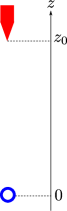
(a) $z_{0}\gg R$

(b) $z_{0}\ll R$

Figure S1: Two simple geometries. Red: micropipette, blue: membrane of the GUV. Denoting by $R$ the radius of the GUV, and by $z_{0}$ the height of the micropipette tip measured from the membrane, these geometries correspond to the asymptotic limits $z_{0}\gg R$ and $z_{0}\ll R$.

In geometry (a), i.e., for $z_{0}\gg R$, we can consider that the acid diffuses freely in an infinite volume in order to calculate the proton concentration $C$. Conversely, in geometry (b), i.e., for $z_{0}\ll R$, we can consider that the membrane imposes a Neumann boundary condition to $C$:

$$\partial_{z}C\left(r,z=0,t\right)=0\,.$$ (6)

This boundary condition, corresponding to complete reflection on the membrane, is fully valid in the stationary state, where the membrane is at chemical equilibrium with the surrounding solution, so that there are as many protons per time unit that adsorb onto the membrane (by reacting with a lipid) as protons that desorb from the membrane. In the transient state at the beginning of the injection, taking this boundary condition amounts to neglecting the excess protons that react with the membrane, which is legitimate given that the membrane is a surface and that the fraction of lipids that react with protons is assumed to remain small. As shown below, the acid concentration on the vesicle can be considered constant during most of the injection phase.

Resolution of the diffusion problem.

The solution to the diffusion equation Eq. (2) can be written as:

$$C\left(r,z,t\right) =\int_{0}^{t}\!\!dt^{\prime}\int_{\mathbb{R}^{2}}\!\!\!\!d\bm{r^{\prime}}\int_{0}^{+\infty}\!\!\!\!\!\!\!\!dz^{\prime}\,\Sigma\left(\bm{r^{\prime}},z^{\prime},t^{\prime}\right)\,G\left(|\bm{r}-\bm{r^{\prime}}|,z,z^{\prime},t-t^{\prime}\right)$$

$$=\Sigma_{0}\int_{0}^{\mathrm{min}(t,\,T)}dt^{\prime}\,G\left(r,z,z_{0},t-t^{\prime}\right)\,,$$ (7)

where $G$ is the causal Green function of the diffusion equation which verifies the appropriate boundary conditions.
In geometry (a), it is simply the infinite-volume causal Green function of the diffusion equation:

$$G_{\infty}\left(r,z,z_{0},t\right)=\frac{\theta(t)}{\left(4\,\pi\,D\,t\right)^{3/2}}\,\exp\left(-\frac{r^{2}+(z-z_{0})^{2}}{4\,D\,t}\right)\,,$$ (8)

where $\theta$ is the Heaviside function.
In geometry (b), the boundary condition Eq. (6) can be accounted for using the method of images (7), yielding:

$$G\left(r,z,z^{\prime},t\right)=G_{\infty}\left(r,z,z^{\prime},t\right)+G_{\infty}\left(r,z,-z^{\prime},t\right)\,.$$ (9)

Using Eqs. (7), (8) and (9), it is possible to obtain explicit analytical expressions for $C(r,z,t)$ in both geometries (6, 8).

Steady-state concentration on the GUV membrane.

Here, we are interested in calculating the pH imposed on the GUV membrane during the injection, which lasts $T\approx 30\,\mathrm{s}$ in our experiments. Since the concentration of protons is determined by diffusion of the acid solution from the micropipette tip, this concentration can be considered to have reached steady state at the point of coordinates $(r,z)$ if the time $t$ from the beginning of the injection verifies $t\gg(r^{2}+(z-z_{0})^{2})/D$. For instance, on the membrane in front of the micropipette, it corresponds to $t\gg z_{0}^{2}/D\approx 30\,\mathrm{ms}$, where we have used the above-mentioned values for $z_{0}$ and $D$. Since this threshold is much smaller than the total injection time $T$, the relevant value of the proton concentration during the injection is that at steady-state.
In the (a) geometry, the steady-state concentration at the membrane surface (i.e., at $z=0$) reads

$$C^{\mathrm{(a)}}\left(r\right)=\frac{\Sigma_{0}}{4\,\pi\,D}\,\,\frac{1}{\sqrt{r^{2}+z_{0}^{2}}}\,,$$ (10)

and in the (b) geometry, it reads

$$C^{\mathrm{(b)}}\left(r\right)=2\,C^{\mathrm{(a)}}\left(r\right)\,.$$ (11)

Note that the twofold difference between cases (a) and (b) directly arises from the method of images (7).

3 pH in front of the micropipette during the experiments

Using Eqs. (10) and (11) together with Eqs. (5) and (1), the acid concentration on the membrane during the experiments can be estimated. We calculate it for the steady state of the injection phase (as explained above), and in front of the micropipette (in $r=0$), because it is where the pH is lowest.

In our experiments, the distance between the micropipette tip and the membrane is $z_{0}=10\,\mu\mathrm{m}$, and the radius $R$ of the GUV is about $25\,\mu\mathrm{m}$. Hence, the actual pH is expected to be comprised between those calculated for the limiting geometries (a) and (b). We carried out the calculations in both cases.

Besides, we took into account the uncertainty on the injection pressure (15-25 hPa), as well as on the effective value of $\ell$, (i.e. the 5-10 $\mu\mathrm{m}$ length over which the micropipette has its smallest diameter $\delta=0.3\,\mu\mathrm{m}$). Calculating the pH from Eqs. (10) and (11) for all these sets of values, yielded two pH extremes, namely 4.4 and 5.2. Hence, it can be concluded that during the microinjection, the pH at the GUV membrane surface, in front of the micropipette, is

$$\mathrm{pH}=4.8\pm 0.4\,.$$ (12)

Since this range of values is more that 2 units below the pKa of Hepes, the effect of the buffer can be neglected.

Additional experimental results

Figure S2: Local membrane invagination triggered on a GUV composed of PC/CL 90:10 mol/mol by a local pH decrease performed using a micropipette delivering an acidic solution (100 mM HCl, pH 1.6) in buffer A at pH 8. The acid microinjection is started at t=0 and ended at t=31.8 s. The corresponding movie is movie S1.

Details of simulation results

Figure S3: A. Dynamics of the growth of tube length $L$ derived from simulations and considering either only a direct equilibrium density change of the outer monolayer (solid line), corresponding to CL-containing GUVs, or both a direct equilibrium density change and transbilayer sink/source flip flop (dashed line), corresponding to CL-containing GUVs. The two vertical dotted lines correspond respectively to the end of the constant local density increase of the outer monolayer (i.e. injection time) and the end of the relaxation of this density increase.
B, C. Dynamics of the fractions of the total dissipated power $D_{tot}$ arising from intermonolayer friction ($D_{b_{m}}$, solid line) and monolayer viscosity dissipation ($D_{\mu}$, dotted line) in the case of only a direct equilibrium density change of the outer monolayer (B), or of both a direct equilibrium density change and transbilayer sink/source flip flop (C).