Simultaneous Embeddability of Two Partitions

Abstract

We study the simultaneous embeddability of a pair of partitions of the same underlying set into disjoint blocks. Each element of the set is mapped to a point in the plane and each block of either of the two partitions is mapped to a region that contains exactly those points that belong to the elements in the block and that is bounded by a simple closed curve. We establish three main classes of simultaneous embeddability (weak, strong, and full embeddability) that differ by increasingly strict well-formedness conditions on how different block regions are allowed to intersect. We show that these simultaneous embeddability classes are closely related to different planarity concepts of hypergraphs. For each embeddability class we give a full characterization. We show that (i) every pair of partitions has a weak simultaneous embedding, (ii) it is -complete to decide the existence of a strong simultaneous embedding, and (iii) the existence of a full simultaneous embedding can be tested in linear time.

1 Introduction

Pairs of partitions of a given set of objects occur naturally when evaluating two alternative clusterings in the field of data analysis and data mining. A clustering partitions a set of objects into blocks or clusters, such that objects in the same cluster are more similar (according to some notion of similarity) than objects in different clusters. There are a multitude of clustering algorithms that use, e.g., an underlying graph structure or an attribute-based distance measure to define similarities. Many algorithms also provide configurable parameter settings. Consequently, different algorithms return different clusterings and judging which clustering is the most meaningful with respect to a certain interpretation of the data must be done by a human expert. For a structural comparison of two clusterings several numeric measures exist [23], however, a single numeric value hardly shows where the clusterings agree or disagree. Hence, a data analyst may want to compare different clusterings visually, which motivates the study of simultaneous embeddability of two partitions.

We provide fundamental characterizations and complexity results regarding the simultaneous embeddability of a pair of partitions. While simultaneous embeddability can generally be defined for any number $k\geq 2$ of partitions, we focus on the basic case of embedding two partitions, which is also the most relevant one in the data analysis application. We propose to embed two alternative partitions of the same set $U$ into the plane $\mathbb{R}^{2}$ by mapping each element of $U$ to a unique point and each block (of either of the two partitions) to a region bounded by a simple closed curve. Each block region must contain all points that belong to elements in that block and no point whose element belongs to a different block. Hence, in total, each point lies inside two block regions.

A simultaneous embedding of two partitions shares certain properties with set visualizations like Euler or Venn diagrams [7, 11, 22]. Its readability will be affected by well-formedness conditions for the intersections of the different block regions. Accordingly, we define a (strict) hierarchy of embeddability classes based on increasingly tight well-formedness conditions: weak, strong, and full embeddability. We show that (i) any two partitions are weakly embeddable, (ii) the decision problem for strong embeddability is -complete, and (iii) there is a linear-time decision algorithm for full embeddability. We fully characterize the embeddability classes in terms of the existence of a planar support (strong embeddability) or in terms of the planarity of the bipartite map (full embeddability). Interestingly, both concepts are closely related to hypergraph embeddings and different notions of hypergraph planarity. Our -completeness result implies that vertex-planarity testing of 2-regular hypergraphs is also -complete.

1.1 Related Work

In information visualization there are a large variety of techniques for visualizing clusters of objects, some of which simply map objects to (colored) points so that spatial proximity indicates object similarity [5, 16], others explicitly visualize clusters or general sets as regions in the plane [8, 22]. These approaches are visually similar to Euler diagrams [7, 11], however, they do not give hard guarantees on the final set layout, e.g., in terms of intersection regions or connectedness of regions, nor do they specifically consider the simultaneous embedding of two or more clusterings or partitions.

Clustered planarity is a concept in graph drawing that combines a planar graph layout with a drawing of the clusters of a single hierarchical clustering. Clusters are represented as regions bounded by simple closed and pairwise crossing-free curves. Such a layout is called c-planar if no edge crosses a region boundary more than once [10].

The simultaneous embedding of two planar graphs on the same vertex set is a topic that is well studied in the graph drawing literature, see the recent survey of Bläsius et al. [1]. In a simultaneous graph embedding each vertex is located at a unique position and edges contained in both graphs are represented by the same curve for both graphs. The remaining (non-shared) edges are embedded so that each graph layout by itself is crossing-free, but edges from the first graph may cross edges in the second graph.

Some of our results and concepts in this paper can be seen as a generalization of simultaneous graph embedding to simultaneous hypergraph embedding if we consider blocks as hyperedges: all vertices are mapped to unique points in the plane and two hyperedges, represented as regions bounded by simple closed curves, may only intersect if they belong to different hypergraphs or if they share common vertices. Several concepts for visualizing a single hypergraph are known [14, 18, 15, 4, 3], but to the best of our knowledge the simultaneous layout of two or more hypergraphs has not been studied.

1.2 Preliminaries

Let $U=\{u_{1},\dots,u_{m}\}$ be a finite universe. A partition $\mathcal{P}=\{B_{1},\dots,B_{n}\}$ of $U$ groups the elements of $U$ into disjoint blocks, i.e., every element $u\in U$ is contained in exactly one block $B_{i}\in\mathcal{P}$. In this paper, we consider pairs $\{\mathcal{P}_{0},\mathcal{P}_{1}\}$ of partitions of the same universe $U$, i.e., each element $u\in U$ is contained in one block of $\mathcal{P}_{0}$ and in one block of $\mathcal{P}_{1}$. In the following we often omit to mention $U$ explicitly.

Let $\mathcal{S}$ be a collection of subsets of $U$. An embedding $\Gamma$ of $\mathcal{S}$ maps every element $u\in U$ to a distinct point $\Gamma(u)\in\mathbb{R}^{2}$ and every set $S\in\mathcal{S}$ to a simple, bounded, and closed region $\Gamma(S)\subset\mathbb{R}^{2}$ such that $\Gamma(u)\in\Gamma(S)$ if and only if $u\in S$. Moreover, we require that each contiguous intersection between the boundaries of two regions is in fact a crossing point $p\in\mathbb{R}^{2}$, i.e., the local cyclic order of the boundaries alternates around $p$. A simultaneous embedding $\Gamma$ of a pair of partitions $\{\mathcal{P}_{0},\mathcal{P}_{1}\}$ is an embedding of the union $\mathcal{P}_{0}\cup\mathcal{P}_{1}$ of the two partitions. We define $R_{B}=\Gamma(B)$ as the block region of a block $B$ and denote its boundary by $\partial R_{B}$. Figure 1 shows examples of simultaneous embeddings in the three different embedding classes to be defined in Section 2.

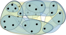
(a) weak embedding

(b) strong embedding

(c) full embedding

Figure 1: Examples of simultaneous embeddings of two partitions.

A simultaneous embedding $\Gamma$ induces a subdivision of the plane and we can derive a plane multigraph $G_{\Gamma}$ by introducing a node for each intersection of two boundaries and an edge for each section of a boundary that lies between two intersections. Furthermore, a boundary without intersections is replaced by a node with a self loop nested inside its surrounding face. We call $G_{\Gamma}$ the contour graph of $\Gamma$ and its dual graph $G_{\Gamma}^{*}$ the dual graph of $\Gamma$. The faces of $G_{\Gamma}$ belong to zero, one, or two block regions. We call a face that belongs to no block region a background face, a face that belongs to a single block region a linking face, and a face that belongs to two block regions an intersection face. Only intersection faces contain points corresponding to elements in the universe, and no two faces of the same type are adjacent in the contour graph.

Alternatively, the union of the two partitions $\mathcal{P}_{0}\cup\mathcal{P}_{1}$ can also be seen as a hypergraph $H=(U,\mathcal{P}_{0}\cup\mathcal{P}_{1})$, where every element $u\in U$ is a vertex and every block defines a hyperedge, i.e., a non-empty subset of $U$. The hypergraph $H$ is 2-regular since every vertex is contained in exactly two hyperedges. We denote $H=H(\mathcal{P}_{0},\mathcal{P}_{1})$ as the corresponding hypergraph of the pair of partitions $\{\mathcal{P}_{0},\mathcal{P}_{1}\}$.

Hypergraph supports [15] play an important role in hypergraph embeddings and their planarity. A support of a hypergraph $H=(V,\mathcal{S})$ is a graph $G_{p}=(V,E)$ on the vertices of $H$, such that the induced subgraph $G_{p}[S]$ of every hyperedge $S\in\mathcal{S}$ is connected. We extend the concept of supports to pairs of partitions, i.e., we say that a graph $G_{p}=(V,E)$ is a support for $\{\mathcal{P}_{0},\mathcal{P}_{1}\}$, if it is a support of $H(\mathcal{P}_{0},\mathcal{P}_{1})$.

We call a support path based, if the induced subgraphs of all hyperedges are paths, and tree based, if all hyperedge-induced subgraphs are trees, i.e., they do not contain any cycles. For any support $G_{p}$ of a pair of partitions $\{\mathcal{P}_{0},\mathcal{P}_{1}\}$ we can always create a tree-based support $G^{\prime}_{p}$ by removing edges from cycles: Suppose there exists a block $B\in\mathcal{P}_{0}$ such that $G_{p}[B]$ contains a cycle $K$. If the vertices in $K$ are also contained in a common block of $\mathcal{P}_{1}$, we can just remove a random edge from $K$ without destroying the support property. Otherwise, we can remove an edge from $K$ that connects vertices in two different blocks of $\mathcal{P}_{1}$ without destroying the support property.

The bipartite map $G_{b}(H)$ of a hypergraph $H=(V,\mathcal{S})$ is defined as the bipartite graph $G_{b}(H)=(V\cup\mathcal{S},E_{b})$ that has a node for each vertex in $V$ and for each hyperedge in $\mathcal{S}$ [24]. A node $v\in V$ is adjacent to a node $S\in\mathcal{S}$ if $v\in S$. We say that $G_{b}(H)$ is the bipartite map of a pair of partitions $\{\mathcal{P}_{0},\mathcal{P}_{1}\}$ if $H=H(\mathcal{P}_{0},\mathcal{P}_{1})$.

Finally, we define the block intersection graph $G_{s}(\mathcal{P}_{0},\mathcal{P}_{1})$ as the graph with vertex set $V_{s}=\mathcal{P}_{0}\cup\mathcal{P}_{1}$ and edge set $E_{s}=\{\{B,B^{\prime}\}\mid B\cap B^{\prime}\neq\emptyset\}$. Thus $G_{s}$ has a vertex for each block and an edge between any two blocks that share a common element. Since only blocks of different partitions can intersect, we know that $G_{s}$ is bipartite.

2 The Main Classes of Embeddability

We define three main concepts of simultaneous embeddability for pairs of partitions. We will see that these concepts induce a hierarchy of embeddability classes of pairs of partitions.

2.1 Weak Embeddability

We begin with weak embeddability, which is the most general concept.

Definition 1 (Weak Embeddability)

A simultaneous embedding of two partitions is weak if no two block regions of the same partition intersect. Two partitions are weakly embeddable if they have a weak simultaneous embedding.

Prohibiting intersections of block regions of the same partition is our first well-formedness condition. A weak embedding emphasizes the fact that the blocks in each partition are disjoint. Since the blocks of any partition are disjoint by definition, it is not surprising that any pair of partitions is weakly embeddable (see Fig. 1(a) for an example).

Theorem 2.1

Any two partitions of a common universe are weakly embeddable on any point set.

Proof

A spanning forest (in fact, any planar graph) on $n$ nodes can always be drawn in a planar way on any fixed set of $n$ points in the plane [19]. Let now $\mathcal{P}$ be a partition. We choose arbitrary, but distinct points in the plane for the elements of $U$. We then generate a spanning tree on the elements in each block and embed the resulting forest in a planar way on the points. Slightly inflating the thickness of the edges of the trees yields simple bounded block regions. We can do this independently for a second partition on the same points and obtain a weak simultaneous embedding.∎

Although the concept of weak embedding does not seem to provide interesting insights into the structure of a given pair of partitions, it guarantees at least the existence of a simultaneous embedding for any pair of partitions that is more meaningful than an arbitrary embedding. An obvious drawback of weak embeddings is that the block regions of disjoint blocks are allowed to intersect, as long as both blocks belong to different partitions—even if they do not share common elements.

2.2 Strong Embeddability

Following the general idea of Euler diagrams [7], which do not show regions corresponding to empty intersections, we establish a stricter concept of embeddability. In a strong embedding block regions may only intersect if the corresponding blocks have at least one element in common, and even more, each intersection face of the contour graph must actually contain a point, see Fig. 1(b). This is our second well-formedness condition.

Definition 2 (Strong Embeddability)

A simultaneous embedding $\Gamma$ of two partitions is strong if each intersection face of the corresponding contour graph contains a point $\Gamma(u)$ for some $u\in U$. Two partitions are strongly embeddable if they have a strong simultaneous embedding.

Obviously, a strong embedding is also weak, since blocks of the same partition have no common elements, and thus, cannot form intersection faces. The class of strongly embeddable pairs of partitions is characterized by Theorem 2.2; we show in Section 3 that deciding the strong embeddability of a pair of partitions is -complete.

Theorem 2.2

A pair of partitions of a common universe is strongly embeddable if and only if it has a planar support.

Proof

Let $\{\mathcal{P}_{0},\mathcal{P}_{1}\}$ be a pair of partitions and let $G_{\Gamma}$ be the contour graph resulting from a strong embedding $\Gamma$ of $\{\mathcal{P}_{0},\mathcal{P}_{1}\}$. We construct a planar support of $\{\mathcal{P}_{0},\mathcal{P}_{1}\}$ along $G_{\Gamma}$ as follows. First recall that the elements of the universe, which correspond to the nodes in a support, are represented in $\Gamma$ by points that are drawn inside intersection faces. Vice versa, since $\Gamma$ is strong, each intersection face contains at least one point. Hence, we choose one point in each intersection face as the center of this face. We now create a dummy vertex for each linking face (observe that one block region may induce several linking faces) and link it to the centers of all adjacent intersection faces. The resulting graph is a subgraph of the dual graph of the contour graph $G_{\Gamma}$ and therefore planar. We now connect all remaining vertices in a star-like fashion to the center of their intersection face, routing the edges in a non-crossing way. We finally remove the dummy vertices by merging them to an adjacent center, linking all adjacent vertices to that center. This graph remains planar. It also has the support property, since all intersection and linking faces of any block region are connected into a single component, and with them all vertices of that block region.

Now we construct a strong embedding from a planarly embedded support of $\{\mathcal{P}_{0},\mathcal{P}_{1}\}$. To this end, we first construct a tree-based support by deleting edges from cycles as described in Section 1.2. Then, we simply inflate the edges of each block-induced subtree. Since the underlying support is embedded in a planar way, this yields a simple block region for every block in $\{\mathcal{P}_{0},\mathcal{P}_{1}\}$ such that two block regions only intersect at the positions of the nodes. Hence, the constructed block regions together with the nodes of the support form a strong embedding of $\{\mathcal{P}_{0},\mathcal{P}_{1}\}$. We note that the support graph as a planar graph can in fact be embedded on any point set [19]. Hence, a strongly embeddable pair of partitions can be strongly embedded on any point set.∎

2.3 Full Embeddability

In a strong embedding, a single block region may still cross other block regions and intersect the same block regions several times forming distinct intersection faces—as long as each intersection face contains at least one common point. The last of our three embeddability classes prevents this behavior and requires that the block regions form a collection of pseudo-disks, i.e., the boundaries of every pair of regions intersect at most twice and the boundaries of two nested regions do not intersect. See Fig 1(c) for an example. This implies in particular that every block intersection is connected, which is a well-formedness condition widely used in the context of Euler diagrams [7], and that block regions do not cross and are thus more locally confined.

Definition 3 (Full Embeddability)

A simultaneous embedding of two partitions is full if it is a strong embedding and the regions form a collection of pseudo-disks. Two partitions are fully embeddable if they have a full simultaneous embedding.

Using a linear-time algorithm for planarity testing [13], the following characterization of fully embeddable pairs of partitions directly implies a linear-time algorithm for deciding full embeddability.

Theorem 2.3

A pair of partitions of a common universe is fully embeddable if and only if its bipartite map is planar.

(a) full embedding

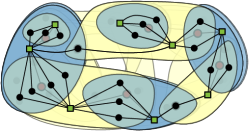
(b) dual of contour graph

(c) final bipartite map

Figure 2: Step-by-step illustration of the proof of Theorem 2.3. Middle: Dual graph of contour graph, nodes in background faces already deleted, additional green nodes for nested regions already inserted.

Proof

Let $\{\mathcal{P}_{0},\mathcal{P}_{1}\}$ be a pair of partitions and $G_{\Gamma}^{*}$ the dual graph of a corresponding full embedding $\Gamma$. The bipartite map of $\{\mathcal{P}_{0},\mathcal{P}_{1}\}$ can be constructed as follows. Remove all vertices (and incident edges) from $G_{\Gamma}^{*}$ that stem from a background face in the contour graph (Fig. 2(a) and Fig. 2(b)). This results in a planar graph with a set of red nodes resulting from intersection faces, a set of green nodes resulting from linking faces and edges indicating that two faces in the contour graph are adjacent. Our definitions of simultaneous embedding and contour graph ensures that nodes of the same color are not adjacent. Hence, the graph constructed so far is bipartite. Moreover, each red node is adjacent to at most two green nodes and, since $\Gamma$ is full (more precisely, since each intersection face in the contour graph is adjacent to at most two linking faces), two green nodes have at most one red common neighbor. From the same fact it further follows that each block region in $\Gamma$ induces at most one linking face in the contour graph, and thus, the number of green nodes is at most the number of blocks in $\{\mathcal{P}_{0}\cup\mathcal{P}_{1}\}$.

If there are fewer green nodes than blocks in $\{\mathcal{P}_{0}\cup\mathcal{P}_{1}\}$, at least one block region in $\Gamma$ must be completely contained in another block region resulting in a red node for the intersection but no green node which could be considered as a representative of the nested block. Hence, the red node representing the intersection is only adjacent to one green node, namely the green node resulting from the linking face of the block region that contains the nested block. Note that no three block regions can be nested, since each point in $\Gamma$ is contained in exactly two block regions. In this case, we link an additional green node to the red node of the nested block region such that in the end each block in $\{\mathcal{P}_{0},\mathcal{P}_{1}\}$ corresponds to a green node and each red node is adjacent to exactly two green nodes. Such an additional leaf obviously preserves planarity (Fig. 2(b)).

Since the bipartite map of a hypergraph (besides the nodes representing blocks) consists of nodes representing the elements in the universe, we finally replace each red node by a set of nodes representing the elements that have been mapped by $\Gamma$ into the corresponding intersection face, and connect each of these new nodes along the previous edges to the two green nodes previously adjacent to the replaced red node. This again preserves planarity of the finally resulting bipartite map of $\{\mathcal{P}_{0}\cup\mathcal{P}_{1}\}$ (Fig. 2(c)).

Now assume a planar embedding of the bipartite map of $\{\mathcal{P}_{0},\mathcal{P}_{1}\}$ with green nodes representing the blocks and black nodes representing the elements of the universe. In order to construct a full embedding of $\{\mathcal{P}_{0},\mathcal{P}_{1}\}$, we first construct for each block in $\{\mathcal{P}_{0},\mathcal{P}_{1}\}$ a subgraph of the bipartite map such that each subgraph contains the green node that represents the corresponding block and two subgraphs share exactly one black node if and only if the corresponding blocks share at least one element. Since the map of $\{\mathcal{P}_{0},\mathcal{P}_{1}\}$ is bipartite, each of these subgraphs is a star with black leaves linked to a green center. Together these stars form a planar subgraph of the bipartite map such that slightly inflating the edges in each star yields simple block regions that intersect exactly at the positions of the black nodes. In the resulting contour graph, two block regions thus intersect at most once and each intersection face is adjacent to exactly two linking faces, each representing a block. A nested block in $\mathcal{P}_{0}\cup P_{1}$ results in a star that only consists of a green center and one black leaf. In order to completely satisfy the condition of a full embedding, we shrink the block regions of nested blocks such that the boundary of the inner block does not intersect the boundary of the outer block. Deleting the green and black nodes and drawing a set of points that represent the common elements of the intersecting blocks in each intersection face finally yields a full embedding.

We note that our construction uses only a single representative element per block intersection. Thus, in contrast to weak and strong embeddings, it is not clear whether a fully embeddable pair of partitions permits a full embedding on any set of points.∎

2.4 Hierarchy of Embeddability Classes

A full embedding is strong by definition and we have seen above that a strong embedding is also weak. Hence, the three embeddability classes introduced in this section induce a hierarchy of embeddability classes. We now show that this hierarchy is strict.

The left side of Fig. 3(a) shows a strong embedding of a pair of partitions $\{\mathcal{P}_{0},\mathcal{P}_{1}\}$ that is not fully embeddable. The dotted lines indicate a planar support proving the strong embeddability of $\{\mathcal{P}_{0},\mathcal{P}_{1}\}$. The fact that $\{\mathcal{P}_{0},\mathcal{P}_{1}\}$ is not fully embeddable can be seen by considering the bipartite map of $\{\mathcal{P}_{0},\mathcal{P}_{1}\}$, which is a subdivision of $K_{3,3}$, and thus, is not planar (see right side of Fig. 3(a)). The claim then follows from Theorem 2.3.

(a) strongly but not fully embeddable

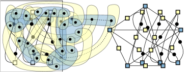
(b) weakly but not strongly embedable

Figure 3: Examples of simultaneous embeddings of two partitions proving the strictness of the hierarchy of embedding classes.

In order to prove that the class of strong embeddability is a proper subclass of weak embeddability, we take a detour via string graphs.

A graph $G=(V,E)$ is a string graph if there exists a set $\mathcal{R}=\{R(v)\mid v\in V\}$ of curves in the plane such that $R(u)\cap R(v)\not=\emptyset$ if and only if $\{u,v\}\in E$. Deciding whether a graph is a string graph is -hard [20]. However, Schaefer and S̆tefankovic̆ [21] showed that a graph is no string graph if it is constructed from a non-planar graph by subdividing each edge at least once. Together with the following lemma we can thus prove that the pair of partitions shown in Fig. 3(b) is not strongly embeddable.

Lemma 1

The block intersection graph of a strongly embeddable pair of partitions is a string graph.

Proof

Let $\Gamma$ be a strong embedding of a pair of partitions $\{\mathcal{P}_{0},\mathcal{P}_{1}\}$. Our goal is to construct a set $\mathcal{R}=\{R(B)\mid B\in\mathcal{P}_{0}\cup\mathcal{P}_{1}\}$ of curves in the plane, which correspond to the blocks in $\mathcal{P}_{0}\cup\mathcal{P}_{1}$ such that $R(B)\cap R(B^{\prime})\not=\emptyset$ if and only if $B$ and $B^{\prime}$ share a common element. This is equivalent to the assertion that the block intersection graph $G_{s}(\mathcal{P}_{0},\mathcal{P}_{1})$ is a string graph. We construct $\mathcal{R}$ along $\Gamma$ as follows. First we delete the points in $\Gamma(U)$. Then we delete one point of the boundary of each block region that is not an intersection point. This results in a set $R$ of curves that correspond to the blocks in $\mathcal{P}_{0}\cup\mathcal{P}_{1}$, and since $\Gamma$ is strong, two curves have a common point if and only if the corresponding blocks have at least one common element and the previous block regions were not nested in $\Gamma$. For blocks whose block regions are nested in $\Gamma$, we replace the curve that represents the nested block by a curve that crosses the surrounding block curve. This finally yields the desired set of curves. ∎

Now consider the pair of partitions in Fig. 3(b). The left side of Fig. 3(b) shows a weak embedding while the right side shows the corresponding block intersection graph, which is constructed from $K_{5}$ by subdividing each edge exactly once. Consequently, since $K_{5}$ is not planar, it is no string graph (according to Schaefer and S̆tefankovic̆ [21]). Applying Lemma 1 finally proves that the pair of partitions depicted in Fig. 3(b) is not strongly embeddable.

2.5 Embeddability and Hypergraph Planarity

The weak embeddability class forms the basis of the hierarchy and contains all pairs of partitions. The strong embeddability class and the full embeddability class are characterized by the existence of a planar support and the planarity of the bipartite map of a pair of partitions, respectively, where the latter directly implies a linear time algorithm for the corresponding decision problem. Moreover, these characterizations reveal close relations to the hypergraph planarity concepts of Zykov and vertex planarity.

A hypergraph $H=(V,\mathcal{S})$ is Zykov-planar [25], if there exists a subdivision of the plane into faces, such that each hyperedge $S\in\mathcal{S}$ can be mapped to a face of the subdivision, and each vertex $v\in V$ can be mapped to a point on the boundary of all faces that represent a hyperedge containing $v$. Walsh [24] showed that a hypergraph is Zykov planar if and only if its bipartite map is planar.

In contrast, a hypergraph $H=(V,\mathcal{S})$ is vertex-planar [14] if there exists a subdivision of the plane into faces, such that every vertex $v\in V$ can be mapped to a face and for every hyperedge $S\in\mathcal{S}$, the interior of the union of all faces of the vertices in $S$ is connected. Kaufmann et al. [15] showed that a hypergraph is vertex planar if and only if it has a planar support. This shows that the class of fully embeddable pairs of partitions is a subclass of Zykov planar hypergraphs, and the class of strongly embeddable pairs of partitions is a subclass of vertex planar hypergraphs.

3 Complexity of Deciding Strong Embeddability

In this section we show the -completeness of testing strong embeddability. As a consequence, testing whether the corresponding hypergraph of a pair of partitions has a planar support is also -complete by Theorem 2.2. This seems not very surprising considering the more general hardness results of Johnson and Pollak [14] and Buchin et al. [4] who showed that deciding the existence of a planar support and a 2-outerplanar support in general hypergraphs is -hard. However, we consider a restricted subclass of 2-regular hypergraphs, thus, the -hardness of our problem does not directly follow from the previous results. Moreover, other special cases, e.g., finding path, cycle, tree, and cactus supports are known to be solvable in polynomial time [14, 4, 2]. Together with the characterization of Theorem 2.2, Theorem 3.1 immediately implies that testing the vertex planarity of a 2-regular hypergraph is -complete.

Theorem 3.1

Deciding the strong embeddability of a pair of partitions is -complete.

The existing hardness results [14, 4] rely on elements that are contained in more than two hyperedges and could not be adapted to our 2-regular setting. Instead we prove the hardness of deciding strong embeddability by a quite different reduction from the -complete problem monotone planar 3Sat [9]. A monotone planar 3Sat formula $\varphi$ is a 3Sat formula whose clauses either contain only positive or only negated literals (we call these clauses positive and negative) and whose variable-clause graph $H_{\varphi}$ is planar. A monotone rectilinear representation (MRR) of $\varphi$ is a drawing of $H_{\varphi}$ such that the variables correspond to axis-aligned rectangles on the x-axis and clauses correspond to non-crossing E-shaped “combs” above the x-axis if they contain only positive variables and below the x-axis otherwise; see Fig. 6(a).

An instance of monotone planar 3Sat is an MRR of a monotone planar 3Sat formula $\varphi$. In the proof of Theorem 3.1 we will construct a pair of partitions $\{\mathcal{P}_{0},\mathcal{P}_{1}\}_{\varphi}$ that admits a strong embedding if and only if $\varphi$ is satisfiable.

For the sake of simplicity, we restrict the class of strong embeddings to the subclass of proper strong embeddings, which is equivalent, as we can argue that a pair of partitions has a strong embedding if and only if it also has a proper one. A strong embedding is proper if the contour graph does not contain background or linking faces that are adjacent to only two other faces. Figure 4 illustrates how background or linking faces violating this condition can be removed, transforming a strong embedding into a proper one.

(a) Removing a linking face.

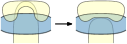
(b) Removing a background face.

Figure 4: Two cases for transforming a strong embedding into a proper strong embedding.

We say that two proper strong embeddings are equivalent if the embeddings of their contour graphs are equivalent, i.e. if the cyclic order of the edges around each vertex is the same. A pair of partitions has a unique strong embedding if all proper strong embeddings are equivalent. Note that, analogously to the definition of equivalence of planar graph embeddings, two equivalent proper strong embeddings may have different unbounded outer background faces. Our construction in the hardness proof is independent of the choice of the outer face.

Next we define a special pair of partitions that has a unique grid-shaped embedding as a scaffold for the gadgets in the subsequent proof of Theorem 3.1. The first step is to construct a base graph $G_{m,n}$ for two integers $m$ and $n$. The graph $G_{m,n}$ is a grid with $mn+1$ columns and $2m+2$ rows of vertices with integer coordinates $(i,j)$ for $0\leq i\leq mn$ and $0\leq j\leq 2m+1$. Each vertex $v$ with coordinates $(i,j)$ is connected to the four vertices at coordinates $(i-1,j),(i+1,j),(i,j-1),(i,j+1)$ (if they exist). Between the middle rows $m$ and $m+1$ we remove all vertical edges except for those in columns $0,m,2m,\dots,nm$. This defines $n$ larger grid cells of width $m$ in this particular row. Figure 5 (left) shows an example.

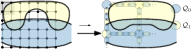
Figure 5: Graph $G_{2,3}$ and the partitions $\{\mathcal{Q}_{0},\mathcal{Q}_{1}\}$ sketched for the top-left grid cell marked in gray.

From $G_{m,n}$ we construct a pair of partitions $\{\mathcal{Q}_{0},\mathcal{Q}_{1}\}$ as follows (see Fig. 5). For each vertex $v$ with coordinates $(i,j)$ we create a vertex block $B_{v}$ in partition $\mathcal{Q}_{(i+j)\pmod{2}}$. For each edge $(u,v)$ in $G_{m,n}$ we create a chain of four edge blocks $B_{u,v}^{1}$, $B_{u,v}^{2}$, $B_{u,v}^{3}$, $B_{u,v}^{4}$, such that $B_{u,v}^{1}$ and $B_{u,v}^{3}$ are in the same partition as $B_{v}$ and $B_{u,v}^{2}$ and $B_{u,v}^{4}$ are in the same partition as $B_{u}$. We distribute five distinct elements among the edge blocks of $(u,v)$ and the vertex blocks for $u$ and $v$ such that they form the desired chain pattern and each intersection face contains one common element. The pair $\{\mathcal{Q}_{0},\mathcal{Q}_{1}\}$ is indeed a pair of partitions as every element belongs to exactly one block of each partition. Edge blocks contain two and vertex blocks up to four elements (depending on the degree of the corresponding vertex in $G_{m,n}$). Below we will add the gadgets of the reduction on top of $\{\mathcal{Q}_{0},\mathcal{Q}_{1}\}$, for which it is required that there is an edge block in each partition that does not share any element with a vertex block. This explains why we link blocks of adjacent vertices by chains of four blocks.

The next lemma shows that $\{\mathcal{Q}_{0},\mathcal{Q}_{1}\}$ has a unique embedding, which is a consequence of the fact that $G_{m,n}$ is a subdivision of a planar 3-connected graph (assuming $n\geq 2$) and thus it has a unique embedding. This property is inherited by $\{\mathcal{Q}_{0},\mathcal{Q}_{1}\}$ in our construction.

Lemma 2

The pair of partitions $\{\mathcal{Q}_{0},\mathcal{Q}_{1}\}$ has a unique embedding.

Proof

First, we observe that the base graph $G_{m,n}$ is a subdivision of a planar 3-connected graph (assuming $n\geq 2$) and thus it has a unique embedding (up to the choice of the outer face) in the plane. We claim that this property is inherited by $\{\mathcal{Q}_{0},\mathcal{Q}_{1}\}$ in our construction.

Each edge block contains exactly two elements and intersects exactly two blocks of the other partition. Thus its contour subgraph in any proper strong embedding is isomorphic to the 4-cycle $C_{4}$ with two non-incident duplicate edges inside, which belong to the boundaries of the two intersecting blocks. Each vertex block $B_{v}$ contains two, three, or four elements, depending on the degree $k$ of $v$ in $G_{m,n}$. Since $B_{v}$ intersects with $k$ edge blocks of the other partition there are exactly two intersection points with the boundary of each of these edge blocks in a proper strong embedding (if there were four intersection points, then the edge block would not be proper). Thus the contour subgraph of $B_{v}$ is a 4-, 6-, or 8-cycle with two, three, or four non-incident duplicate edges inside belonging to the intersecting edge blocks. There is a bijection between the possible cyclic intersection orders of the $k$ edge blocks and the possible cyclic orders of the $k$ incident edges of vertex $v$ in $G_{m,n}$. Thus we have locally the same embedding choices of the contour graph of $C_{v}$ as for the vertex $v$ in $G_{m,n}$. Since $G_{m,n}$ has a unique embedding, and since each edge of $G_{m,n}$ is represented in $\{\mathcal{Q}_{0},\mathcal{Q}_{1}\}$ by a sequence of four edge blocks with a locally unique embedding between the two incident vertex blocks, we conclude that for every proper strong embedding of $\{\mathcal{Q}_{0},\mathcal{Q}_{1}\}$ the induced contour graph is the same graph with the same unique planar embedding. Otherwise we could derive two different embeddings of $G_{m,n}$, which is a contradiction. ∎

Now we have all the tools that we need to prove our main theorem in this section.

Proof (of Theorem 3.1)

First we show that the problem is in . By Theorem 2.2 we know that a pair of partitions is strongly embeddable if and only if it has a planar support. Thus we can “guess” a graph on $U$ and then test its planarity and support property in polynomial time. This shows membership in . It remains to describe the hardness reduction.

Let $\varphi$ be a planar monotone 3Sat formula together with an MRR. First we construct the pair of partitions $\{\mathcal{Q}_{0},\mathcal{Q}_{1}\}$ for the base graph $G_{m,n}$, where $m$ is the number of clauses of $\varphi$ and $n$ is the number of variables of $\varphi$. By Lemma 2 $\{\mathcal{Q}_{0},\mathcal{Q}_{1}\}$ has a unique proper grid-like embedding. We call $\{\mathcal{Q}_{0},\mathcal{Q}_{1}\}$ the base grid and the $n$ special cells between rows $m$ and $m+1$ the variable cells of the base grid.

(a) Monotone rectilinear representation of a formula $\varphi$

(b) Sketch of the clause blocks laid on top of the grid $\{\mathcal{Q}_{0},\mathcal{Q}_{1}\}$ (empty columns omitted)

Figure 6: Illustration of the -hardness reduction

Next we augment the pair of partitions $\{\mathcal{Q}_{0},\mathcal{Q}_{1}\}$ by additional blocks, one for each clause, where positive clauses are added to $\mathcal{Q}_{0}$ and negative clauses to $\mathcal{Q}_{1}$. The definition of these clause blocks closely follows the layout of the given MRR, see Fig. 6(a). Let $C_{1},C_{2},\dots,C_{l}$ be the positive clauses of $\varphi$ ordered so that if $C_{i}$ is nested inside the E-shape of $C_{j}$ in the given MRR then $i<j$. Analogously let $C_{l+1},\dots,C_{m}$ be the ordered negative clauses. We describe the definition of the block $B_{i}$ for a positive clause $C_{i}$ ($1\leq i\leq l$); blocks for negative clauses are defined symmetrically. We create an intermediate embedding of $B_{i}$ (which is not yet strong but serves as a template for a later strong embedding) by putting $B_{i}$ on top of the base grid and adding new elements to $B_{i}$ and to certain edge blocks in $\mathcal{Q}_{1}$. This fixes $B_{i}$ to run through two mirrored E-shaped sets of grid cells of our choice (Fig. 6(b)). In the upper half of the base grid, $B_{i}$ is assigned to run between rows $m-i$ and $m-i+1$. Furthermore, $B_{i}$ is assigned to three columns leading towards the variable cells from the top. Let $x_{j}$ be a variable contained in $C_{i}$ and assume that $C_{i}$ is the $k$-th positive clause from the right connecting to $x_{j}$ in the embedding of the given MRR. Then $B_{i}$ runs between columns $jm-k$ and $jm-k+1$. In the lower half of the base grid we translate and mirror the resulting E-shape as follows. We let $B_{i}$ occupy the cells between rows $2m+2-l+i-1$ and $2m+2-l+i$ and the three columns are shifted to the left by the number of occurrences of the respective variable in negative clauses (Fig. 6(b)). Since each variable cell is $m$ columns wide, we can always assign each clause to a unique column of $x_{j}$ in the top and bottom half of the grid in this way.

We actually fix $B_{i}$ to the base grid by adding one shared element for each crossed edge of a grid cell to both $B_{i}$ and the respective edge block of $\mathcal{Q}_{1}$ that does not share an element with a vertex block in $\mathcal{Q}_{0}$ (recall that $\{\mathcal{Q}_{0},\mathcal{Q}_{1}\}$ contains such a block in each partition and for each grid edge). No two blocks of the same clause type (positive or negative) intersect, but blocks of different type do intersect in certain grid cells. For each grid cell shared between a positive and negative block (except for the $n$ variable cells) we add one shared element (black dots in Fig. 6(b)) and call the respective grid cell the home cell for this element. Recall that the orders of the incoming blocks from the top and the bottom of each variable cell are inverted. Thus, within each variable cell the blocks of each pair of a positive and negative clause using the corresponding variable intersect, but no shared element is added. We denote the resulting new pair of partitions as $\{\mathcal{P}_{0},\mathcal{P}_{1}\}_{\varphi}$ and observe that its size is polynomial in the size of $\varphi$.

Next we argue about the strong embedding options in contrast to the immediate embedding for a clause block $B_{i}$ in $\{\mathcal{P}_{0},\mathcal{P}_{1}\}_{\varphi}$. In the intermediate embedding each block has three connections through variable cells linking the upper E-shape with the lower E-shape. Any element shared with an edge block of the uniquely embedded base grid must obviously be reached by the block region of $B_{i}$. Since the block region must be simple, any strong embedding of $B_{i}$ results from opening the intermediate embedding of $B_{i}$ in exactly two grid cells so that the resulting block region of $B_{i}$ is connected and has no holes. Additionally, a shared element must be placed in any intersection of the block region of $B_{i}$ with block regions of other clause blocks.

First we assume that $\varphi$ is a satisfiable formula and a satisfying variable assignment is given. We need to show that $\{\mathcal{P}_{0},\mathcal{P}_{1}\}_{\varphi}$ has a strong embedding. If a variable $x_{j}$ has the value true in the given assignment we open all blocks of negative clauses using $x_{j}$ in the corresponding variable cell; if $x_{j}$ is false we open all blocks of positive clauses using $x_{j}$. Thus no blocks intersect in variable cells any more. If a clause contains more than one true literal, we open all but one connection in its variable cells of true literals. Since the assignment satisfies $\varphi$, we know that each clause block is opened exactly twice in its variable cells and thus forms a valid simple block region. Moreover, we place all shared elements in their home cells so that every block intersection contains an element and the embedding is strong. We call a strong embedding of $\{\mathcal{P}_{0},\mathcal{P}_{1}\}_{\varphi}$ with the above properties a canonical embedding.

Now assume that $\{\mathcal{P}_{0},\mathcal{P}_{1}\}_{\varphi}$ has a strong embedding. We know that the base grid has its unique embedding and that each block is embedded as a simple region that results from opening the intermediate embedding (with its two E-shapes linked through three variable cells) in exactly two cells. If the embedding is already canonical, we can immediately construct a satisfying variable assignment for $\varphi$: if a variable cell is crossed by clause blocks in $\mathcal{Q}_{0}$ we set the variable to true, otherwise we set it to false. Since every clause block is connected we know that this assignment satisfies all clauses. If the embedding is not canonical we show that it can be transformed into a canonical embedding as follows. In a non-canonical embedding it is possible that two blocks $B_{i}$ and $B_{j}$ intersect in a variable cell $x_{k}$ and have a shared element in their intersection face in the cell of $x_{k}$ rather than in the home cell of that element. This means, on the other hand, that in some shared home cell $\gamma$ of $B_{i}$ and $B_{j}$, say in the upper half, at least one of the two blocks is opened (as there is no more shared element to put into an intersection face). Thus the grid cell $\gamma$ splits the E-shaped block region of one or both blocks in the upper half into two disconnected components, meaning that each opened block crosses at least two variable cells in order to connect both components via the lower half. Hence we can safely split any block that is opened in $\gamma$ in the cell of variable $x_{k}$, re-connect it inside $\gamma$, and place the shared element of $B_{i}$ and $B_{j}$ into its home cell $\gamma$. This removes the block intersection in the cell of $x_{k}$. Once all block crossings within variable cells are removed, the resulting embedding is a canonical embedding and we can derive the corresponding satisfying variable assignment. ∎

4 Extensions and Conclusion

We have characterized three main embeddability classes for pairs of partitions, which in fact form a strict hierarchy, and we have shown -completeness of deciding strong embeddability. From a practical point of view the class of strong embeddings is of particular interest: it guarantees that every intersection between block regions is meaningful as it contains at least one element, but on the other hand allows blocks to cross, imposing less restrictions than full embeddings. Interesting subclasses of strong embeddings that further structure the space between strong and full embeddability can be defined and we mention two of them.

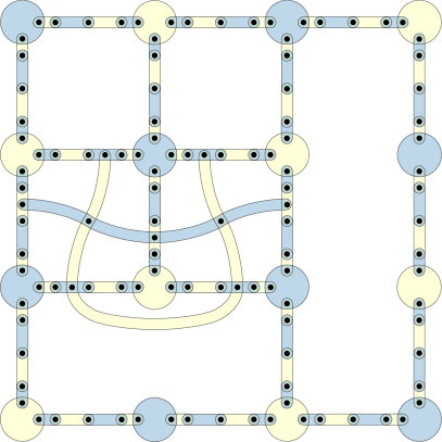
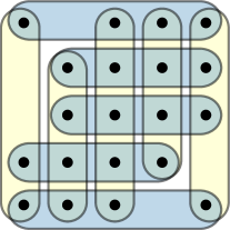
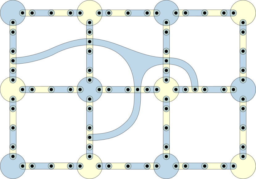
Figure 7: (a) Two partitions based on a uniquely embedded grid that have a strong embedding, but no single-intersection strong embedding. (b) A strong grid embedding. (c) Two partitions based on a uniquely embedded grid that have a single-intersection strong embedding but no strong grid embedding.

In a strong embedding two blocks can intersect many times forming disjoint intersection faces, whereas a full embedding permits only a single connected intersection region for any pair of blocks (this is also a common requirement for Euler diagrams [7]). In single-intersection strong embeddings we adapt this unique intersection region condition of full embeddings, but still permit that two blocks cross in the embedding. This new class is a true subclass of strong embeddings, see the example in Fig. 7. It is open whether the corresponding decision problem is still -complete since our proof is based on the existence of multiple intersection regions between pairs of blocks.

Another interesting subclass are strong grid embeddings, in which the blocks of $\mathcal{P}_{0}$ and $\mathcal{P}_{1}$ are embedded as horizontal and vertical ribbons, respectively, which intersect in a matrix-like fashion, see Fig. 7. Obviously a strong grid embedding is also a single intersection strong embedding, but again strong grid embeddings form a true subclass, see Fig. 7. It is easy to see that a pair of partitions admits a strong grid embedding if and only if its block intersection graph is a grid intersection graph [12], i.e., an intersection graph of horizontal and vertical segments in the plane. Kratochvíl [17] showed that deciding whether a bipartite graph is a grid-intersection graph is -complete. All fully embeddable pairs of partitions have a strong grid embedding: The bipartite map of a fully embeddable pair of partitions is planar by Theorem 2.3 and immediately induces a planar bipartite block intersection graph, which, according to Hartman et al. [12], is a grid intersection graph. This implies -completeness of deciding strong grid embeddability. But as the example of Fig. 3(a) shows, not every instance with a strong grid embedding admits a full embedding.

It is an interesting direction for future work to study the generalization of our embeddability concepts to $k>2$ partitions. While weak embeddability and its properties extend readily to any number of partitions, it is less obvious how to generalize strong and full embeddability. One possibility is to require the properties in a pairwise sense; otherwise constraints for new types of faces in the contour graph belonging to more than one but less than $k$ block regions might be necessary.

On the practical side, future work could be the design of algorithms that find visually appealing simultaneous embeddings according to our different embeddability classes. Finally, if the partitions are clusterings on a graph, one would ideally want to simultaneously draw both the partitions and the underlying graphs.

References

- [1] T. Bläsius, S. G. Kobourov, and I. Rutter. Simultaneous embedding of planar graphs. In R. Tamassia, ed., Handbook of Graph Drawing and Visualization, chapter 11, pp. 349–381. CRC Press, 2013.
- [2] U. Brandes, S. Cornelsen, B. Pampel, and A. Sallaberry. Blocks of hypergraphs: applied to hypergraphs and outerplanarity. In Combinatorial Algorithms (IWOCA’10), vol. 6460 of LNCS, pp. 201–211. Springer, 2011.
- [3] U. Brandes, S. Cornelsen, B. Pampel, and A. Sallaberry. Path-based supports for hypergraphs. J. Discrete Algorithms, 14:248–261, 2012.
- [4] K. Buchin, M. van Kreveld, H. Meijer, B. Speckmann, and K. Verbeek. On planar supports for hypergraphs. In Graph Drawing (GD’09), vol. 5849 of LNCS, pp. 345–356. Springer, 2010. (see also Tech. Rep. UU-CS-2009-035, Utrecht University, 2009)
- [5] A. Buja, D. F. Swayne, M. L. Littman, N. Dean, H. Hofmann, and L. Chen. Data visualization with multidimensional scaling. J. Comput. Graphical Statistics, 17(2):444–472, 2008.
- [6] S. Chaplick, V. Jelínek, J. Kratochvíl, and T. Vyskocil. Bend-bounded path intersection graphs: Sausages, noodles, and waffles on a grill. In Graph-Theoretic Concepts in Computer Science (WG’12), vol. 7551 of LNCS, pp. 274–285. Springer, 2012.
- [7] S. Chow. Generating and Drawing Area-Proportional Euler and Venn Diagrams. PhD thesis, University of Victoria, 2007.
- [8] C. Collins, G. Penn, and S. Carpendale. Bubble sets: Revealing set relations with isocontours over existing visualizations. IEEE TVCG, 15(6):1009–1016, 2009.
- [9] M. de Berg and A. Khosravi. Optimal binary space partitions in the plane. In Computing and Combinatorics (COCOON’10), vol. 6196 of LNCS, pp. 216–225. Springer, 2010.
- [10] Q.-W. Feng, R. Cohen, and P. Eades. Planarity for clustered graphs. In Europ. Symp. Algorithms (ESA’95), vol. 979 of LNCS, pp. 213–226. Springer, 1995.
- [11] J. Flower, A. Fish, and J. Howse. Euler diagram generation. J. Visual Languages and Computing, 19(6):675–694, 2008.
- [12] I. B. A. Hartman, I. Newman, and R. Ziv. On grid intersection graphs. Discrete Mathematics, 87(1):41–52, 1991.
- [13] J. Hopcroft and R. Tarjan. Efficient planarity testing. J. ACM, 21(4):549–568, 1974.
- [14] D. S. Johnson and H. O. Pollak. Hypergraph planarity and the complexity of drawing Venn diagrams. J. Graph Theory, 11(3):309–325, 1987.
- [15] M. Kaufmann, M. van Kreveld, and B. Speckmann. Subdivision drawings of hypergraphs. In Graph Drawing (GD’08), vol. 5417 of LNCS, pp. 396–407. Springer, 2009.
- [16] T. Kohonen. Self-Organizing Maps. Springer, 3rd edition, 2001.
- [17] J. Kratochvíl. A special planar satisfiability problem and a consequence of its \NP-completeness. Discrete Applied Mathematics, 52(3):233–252, 1994.
- [18] E. Mäkinen. How to draw a hypergraph. Int. J. Computer Math., 34(3–4):177–185, 1990.
- [19] J. Pach and R. Wenger. Embedding planar graphs at fixed vertex locations. Graphs and Combinatorics 17(4):717–728, 2001.
- [20] M. Schaefer , E. Sedgwick, and D. S̆tefankovic̆. Recognizing string graphs in NP. Journal of Computer and System Sciences, 67(2):365–380,2003.
- [21] M. Schaefer and D. S̆tefankovic̆. Decidability of string graphs. Journal of Computer and System Sciences, 68(2):319–334,2004.
- [22] P. Simonetto, D. Auber, and D. Archambault. Fully automatic visualisation of overlapping sets. Computer Graphics Forum, 28(3):967–974, 2009.
- [23] S. Wagner and D. Wagner. Comparing Clusterings – An Overview. Tech. Rep. 2006-04, Department of Informatics, Universität Karlsruhe, 2007. http://nbn-resolving.org/urn:nbn:de:swb:90-114774
- [24] T. R. S. Walsh. Hypermaps versus bipartite maps. J. Combinatorial Theory, Series B, 18(2):155–163, 1975.
- [25] A. A. Zykov. Hypergraphs. Russian Mathematical Surveys, 29(6):89–156, 1974.