Universal horizons and black holes in gravitational theories with broken Lorentz symmetry

Abstract

In this paper, we first show that the definition of the universal horizons studied recently in the khronometric theory of gravity can be straightforwardly generalized to other theories that violate the Lorentz symmetry, by simply considering the khronon as a probe field and playing the same role as a Killing vector field. As an application, we study static charged ($D+1$)-dimensional spacetimes in the framework of the healthy (non-projectable) Horava-Lifshitz (HL) gravity in the infrared limit, and find various solutions. Some of them represent Lifshitz space-times with hyperscaling violations, and some have black hole structures. In the latter universal horizons always exist inside the Killing horizons. The surface gravity on them can be either larger or smaller than the surface gravity on the Killing horizons, depending on the space-times considered. Although such black holes are found only in the infrared, we argue that black holes with universal horizons also exist in the full theory of the HL gravity. A simple example is the Schwarzschild solution written in the Painleve-Gullstrand coordinates, which is also a solution of the full theory of the HL gravity and has a universal horizon located inside the Schwarzschild Killing horizon.

I Introduction

Lorentz symmetry has been the cornerstone of modern physics, and verified to such a high accuracy that any modification of it must face one of the most severe experimental constraints existing today in physics Liberati13 , although it is arguable that such constraints in the matter sector are much stronger than those in the gravitational sector LZbreaking . Nevertheless, if space and time emerge from some discrete substratum, as what we currently understand, this symmetry must be an accidental one at low energies.

Following this line of thinking, various gravitational theories that violate Lorentz symmetry have been proposed, ranging from ghost condensation GC , Einstein-aether theory EA , and more recently, to Horava-Lifshitz (HL) gravity Horava . While the ghost condensation and Einstein-aether theory are all considered as the low energy effective theories of gravity, the HL gravity is attempted to be ultraviolet (UV) complete, and by construction is power-counting renormalizable reviews . It is consistent with all the solar system tests carried out so far EA ; KMWZ and binary pulsar observations Yagi , and exhibits various remarkable features when applied to cosmology InflationA ; InflationB ; InflationC ; InflationD .

However, when applying the HL theory to astrophysics, it seems to indicate that black holes are only low energy phenomena KKCP ; GLLSW . This is because, in order to have the theory power-counting renormalizable, high-order spatial operators up to at least sixth-order must be included Horava . Hence, the dispersion relation becomes nonlinear, and generically takes the form reviews ,

$$E^{2}=c_{p}^{2}p^{2}\left(1+\alpha_{1}\left(\frac{p}{M_{*}}\right)^{2}+\alpha_{2}\left(\frac{p}{M_{*}}\right)^{4}\right),$$ (1.1)

where $E$ and $p$ are the energy and momentum of the particle considered, and $c_{p},\;\alpha_{i}$ are coefficients, depending on the particular specie of the particle, while $M_{*}$ denotes the suppression energy scale of the higher-dimensional operators. Then, one can see that both phase and group velocities of the particles are unbounded with the increase of energy. This makes the causal structure of the spacetimes quite different from that given in general relativity (GR), where the light cone of a given point plays a fundamental role in determining its causal structure relative to other events. In the case described by Eq.(1.1), the causal structure is very much similar to the Newtonian case GLLSW . This suggests that black holes may not exist at all in the HL theory, as any ray initially trapped inside a horizon can penetrate it and propagate to infinity, as long as the ray has sufficiently large velocity. On the other hand, in the infrared (IR) the high-order terms are negligible, and the first term in Eq.(1.1) becomes dominant, so one may still define black holes, following what was done in GR .

Surprisingly, in contrast to the above physical intuition, recently it was shown that there still exist absolute causal boundaries, the so-called universal horizons, and particles even with infinitely large velocities would just move around on these boundaries and cannot escape to infinity BS11 . This has immediately attracted lot of attentions UHsA ; UHsB ; BBM ; CLMV ; SVV . In particular, it was shown that the universal horizon radiates like a blackbody at a fixed temperature, and obeys the first law of black hole mechanics BBM . The main idea is as follows: In a given space-time, a timelike foliation parametrized by $\phi\left(x^{\mu}\right)=$ Constant might exist globally. Since the surfaces are timelike, we must have $u^{\lambda}u_{\lambda}=-1$, where $u_{\mu}$ is the normal unit vector of the surface, defined as

$$u_{\mu}=\frac{\phi_{,\mu}}{\sqrt{X}},$$ (1.2)

with $\phi_{,\mu}\equiv\partial\phi/\partial x^{\mu},\;X\equiv-g^{\alpha\beta}\partial_{\alpha}\phi\partial_{\beta}\phi$. The signatures of the metric are $(-1,1,...,1)$. Among these surfaces, there may exist a surface at which $\phi$ diverges, while physically nothing singular happens there, including the metric and the space-time. Given that $\phi$ defines an absolute time, any object crossing this surface from the interior would necessarily also move back in absolute time, which is something forbidden by the definition of the causality in the theory. Thus, even particles with superluminal velocities cannot penetrate this surface, once they are trapped inside it. For more details, we refer readers to BS11 .

In this paper, our purposes are twofold: First, we shall generalize the above definition of the universal horizons to any gravitational theory that may or may not violate the Lorentz symmetry, although such a generalization might be useful only for theories that violate the Lorentz symmetry. In BS11 , $\phi\left(x^{\mu}\right)$ was referred to as the “khronon” field, and considered as describing one degree of freedom of the gravitational field, a spin-0 graviton. To generalize the definition of the universal horizons to other theories, in this paper we shall promote it to the same role as played by a Killing vector of a given space-time, so its existence does not affect the background, but defines the properties of a given space-time. By this way, such a field is no longer part of the underlaid gravitational theory and it may or may not exist in a given space-time, depending on the properties of the space-time considered. Second, we shall find static charged solutions of the healthy extensions of the HL gravity BPS to show that the universal horizons exist in some of these solutions. Such horizons exist not only in the IR limit of the HL gravity, as has been considered so far in BS11 ; UHsA ; UHsB ; BBM ; CLMV ; SVV , but also in the full HL gravity, that is, when high-order operators are not negligible.

The rest of the paper is organized as follows: In Sec. II, we generalize the definition of the universal horizons first discovered in BS11 in the khronometric theory, which is equivalent to the Einstein-aether theory with the hypersurface-orthogonal condition Jacobson10 ; Wang13 , to any theory by considering the khronon field as a probe field, quite similar to a Killing vector field existing in a given space-time, so that whether a khronon field exists or not depends totally on the properties of a given space-time. In Sec. III, we consider charged static spacetimes in the framework of the non-projectable HL gravity in the IR limit, and present various classes of solutions. In Sec. IV, we study the existence of universal horizons in some of the solutions presented in Sec. III, and find that universal horizons indeed exist. The paper is ended with Sec. V, in which we derive our main conclusions and present some discussing remarks. An appendix is also included, in which we briefly review the non-projectable HL gravity in ($D+1$)-dimensional spacetimes when coupled with an electromagnetic field.

It should be noted that electromagnetic static spacetimes in other versions of the HL theory were studied in EMa , while a new mechanism for generation of primordial magnetic seed field in the early universe without the local U(1) symmetry was considered in EMb . However, so far no studies of the existence of the universal horizons have been carried out in these models.

II Causal Structure of Gravitational Theories with Broken Lorentz Symmetry and Universal Horizons

As shown in the last section, once the Lorentz symmetry is broken, the speed of particles can become superluminal, and even instantaneous propagation exists. Then, the causal structure will be quite different from that in theories with Lorentz symmetry, in which light-cones play a central role. It should be noted that the violation of the Lorentz symmetry does not mean the violation of the causality. In fact, in such theory the causality still exists, but different from that given, for example, in GR. In particular, now the causal structure of a given point $p$ is uniquely determined by the time difference, $\Delta{t}\equiv t_{p}-t_{q}$, between the two events $p$ and $q$. If $\Delta{t}>0$, the event $q$ is to the past of $p$; if $\Delta{t}<0$, it is to the future; and if $\Delta{t}=0$, the two events are simultaneous [cf. Fig.1].

Figure 1: (a) The light cone of the event $p$ in GR. (b) The causal structure of the event $p$ in the HL gravity (See also GLLSW ).

As a result, all the definitions of black holes in terms of event horizons HE73 ; Tip77 ; Hay94 ; Wang become invalid, as a particle initially trapped inside such a horizon now can penetrate it and propagate to infinity, as long as its velocity is sufficiently large. To provide a proper definition of black holes, anisotropic conformal boundaries HMT2 and kinematics of particles KM have been studied in the framework of the HL gravity. In particular, defining a horizon as the infinitely redshifted 2-dimensional (closed) surface of massless test particles KKb , it was found that for test particles with sufficiently high energy, the radius of the horizon can be made as small as desired, although the singularities can be seen in principle only by observers with infinitely high energy GLLSW . This is expected, as such horizons are similar to the event horizon defined in GR HE73 .

Remarkably, studying the behavior of a khronon field in the fixed Schwarzschild black hole background,

$$ds^{2}=-\left(1-\frac{r_{s}}{r}\right)dv^{2}+2dvdr+r^{2}d\Omega^{2},$$ (2.1)

where $r_{s}\equiv 2M$, Blas and Sibiryakov showed that a universal horizon exists inside the Schwarzschild radius $r_{s}$ BS11 . This surface, in contrast to the event horizon, now is spacelike, and on which the time-translation Killing vector $\zeta^{\mu}=\delta^{\mu}_{v}$ becomes orthogonal to $u^{\mu}$,

$$u_{\mu}\zeta^{\mu}=0.$$ (2.2)

Since $u_{\mu}$ is well-defined in the whole space-time, and remains timelike from the asymptotical infinity ($r=\infty$) all the way down to the space-time singularity ($r=0$), Eq.(2.2) is possible only inside the Killing horizon ($\zeta^{\lambda}\zeta_{\lambda}=0$), as only there $\zeta^{\mu}$ becomes spacelike and can be possibly orthogonal to $u_{\mu}$.

The khronon defines globally an absolute time, and the trajectory of a particle must be always along the increasing direction of $\phi$. Thus, once the particle across the universal horizon, the only destination is to move towards the space-time singularity, and arrive at it within a finite (proper) time, as shown in Fig.2. From this same figure, one can also see that the normal vector $u_{\mu}$ is pointing outwards for some $\phi$ at the event horizon $r=r_{EH}$. That is, for a particle with a sufficient large velocity (larger than that of light), it can escape from the interior of the event horizon to asymptotically-flat infinities. In particular, near the universal horizon the khronon behaves like BS11 ,

$$\phi\simeq v+\frac{\log(\xi_{UH}-\xi)}{\xi_{UH}^{2}u_{\tau}^{\prime}\sqrt{\xi_{UH}^{2}-1}},$$ (2.3)

where $\xi\equiv r_{s}/r$, and $\xi=\xi_{UH}$ (or $\phi=\infty)$ is the location of the universal horizon. $u_{\tau}$ is the $\tau$-component of the khronon field, and $u_{\tau}^{\prime}\equiv du_{\tau}/d\xi$. Here $\tau$ is the Schwarzschild timelike coordinate, defined as BS11

$$\tau=v-\left[r+r_{s}\ln\left(\frac{r}{r_{s}}-1\right)\right].$$ (2.4)

The hypersurfaces of $\phi=$ Constant are illustrated in Fig.2, from which we can see that these curves are all accumulated to the one $\phi=\infty\;(\xi=\xi_{UH})$, which is the location of the universal horizon and only particles with infinitely large velocities can move around on this surface. A particle inside this surface cannot get out of it, no matter how large its velocity would be.

It should be noted that the singularity of the khronon on the universal horizon is not physical, and can be removed by the gauge transformation,

$$\tilde{\phi}={\cal{F}}(\phi),$$ (2.5)

allowed by the symmetry of the khronon field, where ${\cal{F}}(\phi)$ is an arbitrary monotonic function of $\phi$. In this sense, the khronon is quite different from a usual scalar field.

Figure 2: The foliation of the timelike hypersurfaces $\phi=$ Constant, and the location of the universal horizon $\xi=\xi_{UH}$ on the ($v,r$)-plane. The khronon defines globally an absolute time, and the trajectory of a particle is always along the increasing direction of $\phi$. Thus, once it cross the horizon, the particle move toward the singularity $r=0$ and reaches it within a finite proper time.

To generalize the above definition of the universal horizon to other gravitational theories, one can see that two important ingredients are essential: the existence of the khronon field $\phi\left(x^{\mu}\right)$, and the existence of the asymptotically timelike Killing vector $\zeta^{\mu}$. For a given space-time, the latter can be obtained by solving the Killing equation,

$$D_{\nu}\zeta_{\mu}+D_{\mu}\zeta_{\nu}=0,$$ (2.6)

where $D_{\mu}$ denotes the covariant derivative with respect to the ($D+1$)-dimensional metric $g_{\mu\nu}$.

To find the equation for the khronon, we start with its general action EA ,

$$S_{\phi} = \int d^{D+1}x\sqrt{|g|}\Big{[}c_{1}\left(D_{\mu}u_{\nu}\right)^{2}+c_{2}\left(D_{\mu}u^{\mu}\right)^{2}$$ (2.7)

$$~{}~{}+c_{3}\left(D^{\mu}u^{\nu}\right)\left(D_{\nu}u_{\mu}\right)-c_{4}a^{\mu}a_{\mu}\Big{]},$$

where $a_{\mu}\equiv u^{\alpha}D_{\alpha}u_{\mu}$, and $c_{i}$’s are arbitrary constants. It should be noted that the above action is the most general one in the sense that the resulting differential equations in terms of $u_{\mu}$ are second-order EA . However, when $u_{\mu}$ is hypersurface-orthogonal, that is, when $u_{\mu}$ satisfies the relation,

$$u_{[\nu}D_{\alpha}u_{\beta]}=0,$$ (2.8)

only three of them are independent , as in this case we have the identity EA ,

$$\Delta{\cal{L}}_{\phi}\equiv a^{\mu}a_{\mu}-\big{(}D_{\alpha}u_{\beta}\big{)}\big{(}D^{\alpha}u^{\beta}\big{)}+\big{(}D_{\alpha}u_{\beta}\big{)}\big{(}D^{\beta}u^{\alpha}\big{)}=0.$$ (2.9)

Then, one can always add the term,

$$\Delta{S}_{\phi}=\alpha\int{\sqrt{|g|}\;d^{D+1}x\Delta{\cal{L}}_{\phi}},$$ (2.10)

into $S_{\phi}$, where $\alpha$ is an arbitrary constant. This is effectively to shift the coupling constants $c_{i}$ to ${c}_{i}^{\prime}$, where

$${c}_{1}^{\prime}=c_{1}+\alpha,\;{c}_{2}^{\prime}=c_{2},\;{c}_{3}^{\prime}=c_{3}-\alpha,\;{c}_{4}^{\prime}=c_{4}-\alpha.$$ (2.11)

Thus, by properly choosing $\alpha$, one can always set one of $c_{1,3,4}$ to zero. However, in the following we shall leave this possibility open.

Hence, the variation of $S_{\phi}$ with respect to $\phi$ yields the khronon equation,

$$D_{\mu}{\cal{A}}^{\mu}=0,$$ (2.12)

where Wang13 ,

$${\cal{A}}^{\mu} \equiv \frac{\left(\delta^{\mu}_{\nu}+u^{\mu}u_{\nu}\right)}{\sqrt{X}}\AE^{\nu},$$

$$\AE^{\nu} \equiv D_{\gamma}J^{\gamma\nu}+c_{4}a_{\gamma}D^{\nu}u^{\gamma},$$

$$J^{\alpha}_{\;\;\;\mu} \equiv \big{(}c_{1}g^{\alpha\beta}g_{\mu\nu}+c_{2}\delta^{\alpha}_{\mu}\delta^{\beta}_{\nu}+c_{3}\delta^{\alpha}_{\nu}\delta^{\beta}_{\mu}$$ (2.13)

$$~{}~{}~{}-c_{4}u^{\alpha}u^{\beta}g_{\mu\nu}\big{)}D_{\beta}u^{\nu}.$$

Eq.(2.12) is a second-order differential equation for $u_{\mu}$, and to uniquely determine it, two boundary conditions are needed. These two conditions can be chosen as follows BS11 : (i) One of them is to require it to be aligned asymptotically with the timelike Killing vector,

$$u^{\mu}\propto\zeta^{\mu}.$$ (2.14)

(ii) The second condition can be that the khronon has a regular future sound horizon, which is a null surface of the effective metric EJ ,

$$g^{(\phi)}_{\mu\nu}=g_{\mu\nu}-\left(c_{\phi}^{2}-1\right)u_{\mu}u_{\nu},$$ (2.15)

where $c_{\phi}$ denotes the speed of the khronon .

With the above definition of the universal horizon, several comments now are in order. First, the above definition does not refer to any particular theory of gravity. Therefore, it is applicable to any theory that violates the Lorentz symmetry, including the Einstein-aether theory EA and the HL gravity Horava . But, there is a fundamental difference between the khronon introduced in this paper and the one (a particular aether field with hypersurface-orthognal condition) considered in BS11 ; UHsA ; UHsB ; BBM . In this paper, the khronon plays the same role as a Killing vector field $\zeta^{\mu}$, both of them describe only some properties of a given space-time and have no effects on the given space-time. But, in BS11 ; UHsA ; UHsB ; BBM the khronon was considered as a part of the gravitational field, although in some cases their effects on the gravitational fields were assumed to be negligible. Second, in the literature it has been often considered that the Einstein-aether theory with the hypersurface-orthogonal condition (2.8) is equivalent to the non-projectable HL gravity in the low energy limit. This is incorrect, as the two theory have different gauge symmetries, and they are equivalent only with a particular choice of the gauge, the $T$-gauge, in which the aether $u_{\mu}$ is aligned with the time coordinate $t$, that is, choosing $t=\phi$, as shown explicitly in Jacobson10 ; Wang13 . In the following, we shall refer to these coordinates as the $T$-coordinates. In particular, the Einstein-aether theory is gauge-invariant under the general coordinate transformations,

$$t=\xi^{0}\left(t^{\prime},{x^{\prime}}^{k}\right),\;\;\;x^{i}=\xi^{i}\left(t^{\prime},{x^{\prime}}^{k}\right),$$ (2.16)

where $\xi^{\mu}$ are arbitrary functions of their indicated arguments. While the HL gravity is gauge-invariant only under the foliation-preserving diffeomorphism,

$$t=f\left(t^{\prime}\right),\;\;\;x^{i}=\xi^{i}\left(t^{\prime},{x^{\prime}}^{k}\right).$$ (2.17)

A typical example is the Schwarzschild space-time written in the Painleve-Gullstrand coordinates PG ,

$$ds^{2}=-dt^{2}+\left(dr+\sqrt{\frac{r_{s}}{r}}dt\right)^{2}+r^{2}d\Omega^{2}.$$ (2.18)

This solution is also a solution of the HL gravity (not only in the IR but also in the UV as now $R_{ij}=0$ and all high-order operators of $R_{ij}$ vanish) GLLSW , but the one given by Eq.(2.1) is not. This is because theses two solutions are connected by the coordinate transformations,

$$dt=dv-\frac{dr}{1+\sqrt{\frac{r_{s}}{r}}},$$ (2.19)

which are forbidden by the gauge transformations of Eq.(2.17), although they are allowed by the ones of Eq.(2.16). Therefore, in the Einstein-aether theory these two solutions describe the same space-time, but in the HL gravity they do not, as they are not connected by any coordinate transformations allowed by its gauge symmetry (2.17). More examples of this kind can be found in CW .

Therefore, the Einstein-aether theory with the hypersurface-orthogonal condition is equivalent to the non-projectable HL gravity in the low energy limit only in the $T$-coordinates, in which the timelike foliations of the space-time fixed in the HL gravity coincide with the spacelike hypersurfaces $\phi(x^{\mu})=$ Constant .

The equivalence shown in Jacobson10 is actually the equivalence between the Einstein-aether theory with the hypersurface-orthogonal condition (2.8) and the khronometric theory BPS , as both of them are gauge-invariant under the general covariant coordinate transformations (2.16) and have the same degree of freedom. For more details, we refer readers to Jacobson10 ; Wang13 ; BS11 .

As an application of the universal horizons defined above, in the next section we shall find static charged solutions in the framework of the HL gravity without the projectability condition in the low energy limit BPS . In Sec. V, we study their local and global properties, by paying particular attention to the existence of the universal horizons.

III Static charged Lifshitz-type Solutions in non-projectable $(D+1)$-dimensional HL Gravity

The non-projectable HL gravity in (D+1)-dimensional space-time is briefly reviewed in Appendix A, in which all the field equations are derived, including the generalized Maxwell equations.

In this paper, we shall study static spacetimes described by,

$$N=r^{z}f(r),\;\;\;N^{i}=0,$$

$$g_{ab}dx^{a}dx^{b}=\frac{g^{2}(r)}{r^{2}}dr^{2}+r^{2}\delta_{ij}dx^{i}dx^{j},$$

$$A_{0}=A_{0}(r),\;\;\;A_{r}=A_{1}(r),\;\;\;A_{i}=0,$$ (3.1)

in the coordinates ($t,r,x^{k}$), where $D=d+1,\;(i,j,k=1,2,...,d)$, and $z$ is a constant. The $D-$dimensional Ricci scalar curvature is given by

$$R=2d\frac{rg^{\prime}(r)}{g^{3}(r)}-\frac{d(d+1)}{g^{2}(r)}.$$ (3.2)

In the IR limit, all the operators higher than order 2 can be safely ignored, as mentioned above. Then, from the Maxwell equations (A.16) and (V.1), we obtain

$$A_{1}\alpha_{0}^{\prime}=0,$$ (3.3)

$$\frac{A_{0}^{\prime\prime}}{A_{0}^{\prime}}-\frac{g^{\prime}}{g}-\frac{f^{\prime}}{f}+\frac{d+1-z}{r}=0.$$ (3.4)

Thus, $\alpha_{0}=\alpha_{0}(A^{1}A_{1})$ must be a constant. Then, from Eqs.(A.4) and (A.5) we can see that now $\alpha_{0}$ acts like a cosmological constant, and can be absorbed to $\Lambda$. Therefore, without loss of the generality, we shall set $\alpha_{0}=0$ in the rest of the paper. On the other hand, from Eq.(3.4) we find that,

$$A^{\prime}_{0}=\frac{q}{r^{d+1-z}}f(r)g(r),$$ (3.5)

where $q$ is an integration constant.

Substituting the above ADM variables and $A_{0}$ into the rest of field equations, we find that the momentum constraint vanish directly, but the Hamiltonian constraint and $(r,r)$- and $(i,i)$-components of the dynamical equations are non-trivial. It can be shown that the $(i,i)$-component of the dynamical equations can be derived from the Hamiltonian constraint and the $(r,r)$-component. Therefore, in the current case there are only two independent field equations, after integrating out the electromagnetic field equations (3.3) and (3.4), which are sufficient to determine the two unknown functions $f(r)$ and $g(r)$. The Hamiltonian constraint and the $(r,r)$-component of the dynamical equations are given, respectively, by

$$-2r^{2}\beta\frac{f^{\prime\prime}}{f}+\left(2r^{2}\beta\frac{g^{\prime}}{g}-2r(d+1+z)\beta\right)\frac{f^{\prime}}{f}$$

$$+2r(z\beta+d\gamma_{1})\frac{g^{\prime}}{g}+\left(2\Lambda+\frac{q^{2}}{2g_{e}^{2}r^{2d}}\right)g^{2}$$

$$+r^{2}\beta\frac{f^{\prime 2}}{f^{2}}-2dz\beta-z^{2}\beta-d(d+1)\gamma_{1}=0,$$ (3.6)

$$\frac{r^{2}\beta}{2}\frac{f^{\prime 2}}{f^{2}}+(z\beta+d\gamma_{1})r\frac{f^{\prime}}{f}+\frac{z^{2}\beta}{2}+dz\gamma_{1}$$

$$-\left(\Lambda+\frac{q^{2}}{4g_{e}^{2}r^{2d}}\right)g^{2}+\frac{d}{2}(d-1)\gamma_{1}=0,~{}~{}~{}$$ (3.7)

where

$$\Lambda\equiv\frac{\gamma_{0}\zeta^{2}}{2}.$$ (3.8)

To solve the above equations, we first note that Eq.(III) can be cast in the form,

$$2d\beta\gamma_{1}W+\beta^{2}W^{2}-d^{2}\gamma_{1}^{2}(r_{*}^{2}-1)=0,$$ (3.9)

where

$$r_{*}(r) \equiv \sqrt{r_{s}^{2}+\frac{2\beta g^{2}}{d^{2}\gamma_{1}^{2}}\left(\Lambda+\frac{2q^{2}}{8g_{e}^{2}r^{2d}}\right)},$$

$$W(r) \equiv z+r\frac{f^{\prime}(r)}{f(r)},$$

$$r_{s}^{2} \equiv 1-\frac{(d-1)\beta}{d\gamma_{1}}.$$ (3.10)

Inversely, we find that

$$g^{2}=\frac{d^{2}\gamma_{1}^{2}}{2\beta}\left(r_{*}^{2}-r_{s}^{2}\right)\left(\Lambda+\frac{2q^{2}}{8g_{e}^{2}r^{2d}}\right)^{-1}.$$ (3.11)

From Eq.(3.9), we obtain

$$W=s\frac{1+\epsilon r_{*}(r)}{1-s},$$ (3.12)

where $\epsilon=\pm 1$, and

$$s\equiv\frac{d\gamma_{1}}{d\gamma_{1}-\beta}.$$ (3.13)

Then, from the stability conditions (A.24), we get

$$1\leq s<\frac{d-1}{d-2},$$ (3.14)

which implies that

$$0<r_{s}\leq 1,$$ (3.15)

where the equality holds only when $\beta=0$ or $s=1$.

When $s\not=1$, inserting Eq.(3.12) into the Hamiltonian constraint, we obtain a master equation for $r_{*}(r)$,

$$\frac{2dq^{2}r_{*}}{2q^{2}+C_{2}r^{2d}}+\frac{rsr_{*}^{2}r_{*}^{\prime}}{1-d+(d-2)s+sr_{*}^{2}}$$

$$=\epsilon\left(\frac{1}{1-s}-2+d\right)+\left(d+\frac{s}{1-s}\right)r_{*}+rr_{*}^{\prime},$$ (3.16)

which can be further rewritten as

$$(s-1)rr^{\prime}_{*}+\Delta(r)\left(r^{2}_{*}-r_{s}^{2}\right)\left(r_{*}+\epsilon{\cal{D}}(r)\right)=0,$$ (3.17)

where $\Delta={s}/{\cal D}$, and

$${\cal{D}} \equiv \frac{[(d-1)+(2-d)s][2q^{2}+C_{2}r^{2d}]}{2q^{2}s+C_{2}r^{2d}[d+(1-d)s]},$$

$$C_{2} \equiv 8g_{e}^{2}\Lambda.$$ (3.18)

When $q=0$, we find that

$${\cal{D}} = \frac{d\gamma_{1}-(d-1)\beta}{d(\gamma_{1}-\beta)},\;(q=0),$$ (3.19)

which reduces to the case considered in SLWW ; LSWW . So, in the rest of the paper we consider only the case $q\not=0$. Unlike the case without the electromagnetic field, now it is found difficult to find the general solutions of Eq.(3.17). Therefore, in the following we consider some particular cases.

III.1 $s=1$

When $s=1$, from Eq.(3.13) we find that this implies $\beta=0$. Then, the stability and ghost-free conditions require

$$\lambda=1,\;(\beta=0)$$ (3.20)

as one can see from Eq.(A.20). Therefore, whenever we consider the case $s=1$ (or $\beta=0$) we always assume that $\lambda=1$. To study the solutions further, we consider the two cases $d\not=1$ and $d=1$, separately.

III.1.1 $d\geq 2$

Then, we find Eqs.(III) and (III) reduce to

$$2rd\gamma_{1}\frac{g^{\prime}}{g}+\left(2\Lambda+\frac{q^{2}}{2g_{e}^{2}r^{2d}}\right)g^{2}$$

$$~{}~{}~{}~{}~{}~{}~{}~{}~{}~{}~{}~{}-d(d+1)\gamma_{1}=0,$$ (3.21)

$$d\gamma_{1}r\frac{f^{\prime}}{f}+dz\gamma_{1}+\frac{d}{2}(d-1)\gamma_{1}$$

$$~{}~{}~{}~{}~{}~{}~{}~{}~{}~{}~{}-\left(\Lambda+\frac{q^{2}}{4g_{e}^{2}r^{2d}}\right)g^{2}=0,$$ (3.22)

from which we get

$$g^{2} = 4g_{e}^{2}d(d^{2}-1)\gamma_{1}r^{2d+1}\big{[}(d-1)r^{d}(C_{2}r^{d+1}$$

$$+4g_{0}g_{e}^{2}d(d+1)\gamma_{1})-2q^{2}(d+1)r\big{]}^{-1},$$

$$f = f_{0}g^{-1}r^{1-z},$$ (3.23)

where $f_{0}$ and $g_{0}$ are two integration constants. Rescaling $t\rightarrow f_{0}^{-1}t$, the metric can be cast in the form,

$$ds^{2}=-F(r)dt^{2}+\frac{dr^{2}}{F(r)}+r^{2}\delta_{ij}dx^{i}dx^{j},~{}~{}~{}~{}$$ (3.24)

where

$$F(r)=-\frac{2m}{r^{d-1}}+\frac{Q^{2}}{r^{2d-2}}-\frac{2\Lambda_{e}r^{2}}{d(d+1)},$$ (3.25)

with $g_{0}\equiv-2m$, and

$$Q^{2}\equiv\frac{q^{2}}{2|\gamma_{1}|g_{e}^{2}d(d-1)},\;\;\;\Lambda_{e}\equiv\frac{\Lambda}{|\gamma_{1}|}.$$ (3.26)

Note that in writing the above expressions we had used the fact

$$\gamma_{1}<0,\;(d\geq 2)$$ (3.27)

as one can see from Eq.(A.25). The corresponding Ricci scalar of the surfaces $t=$ Constant is given by

$$R=-\frac{r^{2d}C_{2}+2q^{2}}{4g_{e}^{2}\gamma_{1}r^{2d}},$$ (3.28)

which is singular at $r=0$ when $q\not=0$. On the other hand, the $(d+2)$-dimensional Ricci scalar is given by

$${}^{(d+2)}R = -F^{\prime\prime}-2d\frac{F^{\prime}}{r}-d(d-1)\frac{F}{r^{2}}$$ (3.29)

$$= 2\frac{d+2}{d}\Lambda_{e}-(d-2)(d-1)\frac{q^{2}}{r^{2d}},$$

which is also only singular at $r=0$, provided that $q\not=0$.

The above solutions are nothing but the topologically Reissner-Nordstrom (anti-) de Sitter solutions, and the Penrose diagrams have been given for various possibilities for $d=2$ in Yumei . It can be shown that these diagrams can be easily generalized to the case with any $d$.

III.1.2 $d=1$

In this case, since $\lambda=1$, from Eq.(A.29) we find that

$$\gamma_{1}\;\;{\mbox{is arbitrary}},\;(d=1)$$ (3.30)

and can take any of real values. Thus, from Eqs.(III) and (III) we find that

$$f = f_{0}r^{-z}\sqrt{\left|C_{2}r^{2}+8g_{e}^{2}\gamma_{1}g_{0}+4q^{2}\ln(r)\right|},$$

$$g^{2} = \frac{8g_{e}^{2}\gamma_{1}r^{2}}{C_{2}r^{2}+8g_{e}^{2}\gamma_{1}g_{0}+4q^{2}\ln(r)}.$$ (3.31)

Then, after rescaling the coordinate $t$, the metric can be cast in the form,

$$ds^{2}=-{{F}}(r)dt^{2}+\frac{dr^{2}}{{{F}}(r)}+r^{2}dx^{2},~{}~{}~{}~{}$$ (3.32)

but now with

$${{F}}(r)=-M+A\ln(r)+Br^{2},$$ (3.33)

where

$$M\equiv-g_{0},\;\;\;{{A}}\equiv\frac{q^{2}}{2\gamma_{1}g_{e}^{2}},\;\;\;{{B}}\equiv\frac{\Lambda}{\gamma_{1}}.$$ (3.34)

The corresponding 2d Ricci scalar is given by

$$R=-\frac{{{A}}+2{{B}}r^{2}}{r^{2}},$$ (3.35)

which is singular only at $r=0$ for $A\not=0$. The nature of this singularity depends on the signs of $B$. In particular, when $B>0$ and $A<0$, the above solutions are identical to the charged Banados-Teitelboim-Zanelli (BTZ) black hole BTZ with

$$\left(M,Q,\Lambda_{e}\right)=\left(-g_{0},\sqrt{-A},-B\right),$$ (3.36)

where $M,\;Q$ and $\Lambda_{e}$ denotes, respectively, the BTZ black hole mass, charge, and the the effective cosmological constant.

But, the solutions of Eq.s(3.33) are more general than the charged BTZ black hole. In particular, $A$ is not necessarily negative, as now $\gamma_{1}$ is a free parameter. To study these solutions further, we consider the cases $B>0$, $B=0$ and $B<0$, separately.

Case i) $B>0$. In this case, one can see that the space-time is always asymptotically anti-de Sitter. However, depending on the signs of $A$, the solutions can have different properties. To see these clearly, let us consider the cases $A>0$, $A=0$ and $A<0$, separately.

Case i.1) $B>0,\;A>0$: In this case, we find that

$$\gamma_{1}>0,\;\Lambda>0,$$ (3.37)

for which we have

$${{F}}(r)=\cases{-\infty,&$r=0$,\cr<0,&$r<r_{EH}$,\cr 0,&$r=r_{EH}$,\cr>0,&$r>r_{EH}$,\cr\infty,&$r=\infty$,\cr}$$ (3.38)

where $r_{EH}$ is the unique real root of ${{F}}(r)=0$, as shown in Fig. 3. Thus, in this case the singularity is covered by the Killing horizon located at $r=r_{EH}$. The space-time is asymptotically anti-de Sitter with the effective cosmological constant given by $\Lambda_{\mbox{\small eff}}=-B$. The surface gravity on the Killing horizon is given by

$$\kappa_{EH}=\frac{B(r_{EH}^{2}+r_{c}^{2})}{r_{EH}},$$ (3.39)

which is always positive, where $r_{c}\equiv\sqrt{A/(2B)}$.

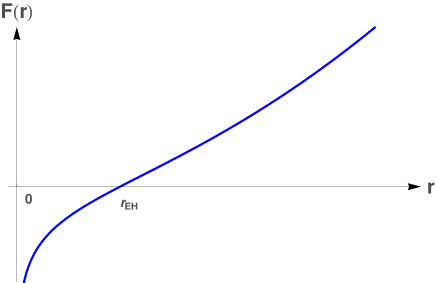
Figure 3: The function ${{F}}(r)$ defined in Eq.(3.33) vs $r$ for $B>0$ and $A>0$, where $r=r_{EH}$ represents the Killing (event) horizon of the black hole. The space-time is singular at $r=0$.

Case i.2) $B>0,\;A=0$: In this case, we have $q=0$, and the corresponding solutions are not charged. Then, we find,

$${{F}}(r)=-M+Br^{2}=\cases{-M,&$r=0$,\cr 0,&$r=r_{EH}$,\cr\infty,&$r=\infty$,\cr}$$ (3.40)

where $r_{EH}\equiv\sqrt{M/B}$. The surface gravity on the Killing horizon now is given by

$$\kappa_{EH}=\sqrt{BM}.$$ (3.41)

Case i.3) $B>0,\;A<0$: In this case, we find

$$\gamma_{1}<0,\;\;\;\Lambda<0,$$ (3.42)

and $F(r)\rightarrow\infty$ for both $r\rightarrow 0$ and $r\rightarrow\infty$. Thus, depending on the values of $B$ (or $\Lambda$), the equation $F(r)=0$ can have two, one or none real roots. In particular, we have $F^{\prime}(r)=-2B(r^{2}-r_{m}^{2})/r$, where $r_{m}\equiv\sqrt{|A|/(2B)}$. Thus, we find

$$F(r_{m}) = \frac{|A|}{2}\left[\ln\left(\frac{2B}{|A|}\right)+1\right]-M$$ (3.43)

$$= \cases{>0,&$\Lambda<\Lambda_{c}$,\cr=0,&$\Lambda=\Lambda_{c}$,\cr<0,&$0>\Lambda>\Lambda_{c}$,\cr}$$

where

$$\Lambda_{c}\equiv-\frac{1}{2}|\gamma_{1}A|e^{\frac{2M-|A|}{|A|}}.$$ (3.44)

Then, the behavior of $F(r)$ is illustrated in Fig.4, from which we can see that the singularity at $r=0$ is naked in Case (a), in which we have $\Lambda<\Lambda_{c}$. In case (c), where $0>\Lambda>\Lambda_{c}$, there exist two Killing horizons, located, respectively, at $r=r_{-}$ and $r=r_{+}$. In this case, the Penrose diagram is similar to the Reissner-Nordstrom anti-de Sitter solutions. In particular, the surface gravity is negative at $r=r_{-}$, while positive at $r=r_{+}$, as one can see from Fig. 4. In Case (b), the two horizons become degenerate, and the surface gravity is zero.

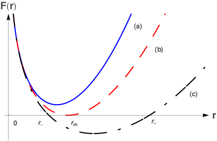
Figure 4: The function ${{F}}(r)$ defined in Eq.(3.33) vs $r$ for $B>0$ and $A<0$: (a) $\Lambda<\Lambda_{c}$; (b) $\Lambda=\Lambda_{c}$; and (c) $0>\Lambda>\Lambda_{c}$, where $\Lambda_{c}$ is defined in Eq.(3.44).

Case ii) $B=0$. In this case, we find that

$$F(r)=-M+A\ln(r).$$ (3.45)

Thus, depending on the values of $A$, the solutions can have different properties. In particular, when $A>0$ ($A<0$) the function $F(r)$ is monotonically increasing (deceasing) as shown in Fig. 5. Then, there always exists a point $r_{EH}$ at which $F(r_{EH})=0$. The surface gravity on this Killing horizon is positive for $A>0$ and negative for $A<0$. When $A=0$, the space-time is flat.

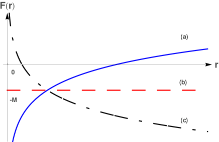
Figure 5: The function ${{F}}(r)$ defined in Eq.(3.33) vs $r$ for $B=0$: (a) $A>0$; (b) $A=0$; and (c) $A<0$.

Case iii) $B<0$: In this case, we have

$${{F}}^{\prime}(r) = 2|B|\frac{r_{m}^{2}-r^{2}}{r},$$

$${{F}}(r_{m}) = -M+\frac{A}{2}\left[\ln\left(\frac{A}{2|B|}\right)-1\right]$$ (3.46)

$$= \cases{>0,&$|B|<B_{m}$,\cr=0,&$|B|=B_{m}$,\cr<0,&$|B|>B_{m}$,\cr}$$

where

$$r_{m}\equiv\sqrt{\frac{A}{2|B|}},\;\;\;B_{m}\equiv\frac{1}{2}Ae^{\frac{-(2M+A)}{A}}.$$ (3.47)

Fig. 6 shows the curve of ${{F}}(r)$ vs $r$. In the case $|B|>B_{m}$, we can see that ${{F}}(r)$ is always negative, and the coordinate $r$ is timelike, and the corresponding space-time is dynamical, and has a spacelike naked singularity at $r=0$.

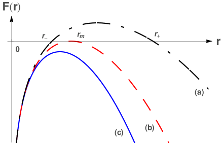
Figure 6: The function ${{F}}(r)$ defined in Eq.(3.33) vs $r$ for $B<0$ and $A>0$. (a) $|B|<B_{m}$; (b) $|B|=B_{m}$; and (c) $|B|>B_{m}$; where $B_{m}$ is defined in Eq.(3.47).

In the case $|B|=B_{m}$, a coordinate singularity appears at $r=r_{m}$, as it can be seen from Eq.(3.35), which now takes the form,

$$R=-2|B|\frac{r_{m}^{2}-r^{2}}{r^{2}}.$$ (3.48)

Therefore, in order to obtain a geodesically maximal space-time, extension across this surface is needed. Such an extension is quite similar to the one of the extremal case, $9\Lambda m^{2}=1$, of the Schwarzschild-de Sitter solution, $F(r)=1-2m/r-\Lambda r^{2}/3$. The corresponding surface gravity is zero, as it can be seem from Eq.(III.1.2).

In the case $|B|<B_{m}$, ${{F}}(r)$ is positive only for $r_{-}<r<r_{+}$, where $r_{\pm}$ are the two real roots of ${{F}}(r)=0$, with $r_{+}>r_{-}$. From Eq.(3.48) we can see that the singularities at $r=r_{\pm}$ represent horizons, and the extensions beyond these horizons are similar to the Schwarzschild–de Sitter solution with $0<\Lambda<1/(9m^{2})$. The corresponding surface gravity is given by

$$\kappa_{\pm}=|B|\frac{r_{m}^{2}-r_{\pm}^{2}}{r_{\pm}},$$ (3.49)

which is positive only when $r_{m}>r_{\pm}$.

It should be noted that the above analysis holds only for $A>0$.

When $A=0$, we have $F(r)=-M-|B|r^{2}<0$, and the solutions represent dynamical space-time, in which $r$ ($t$) is always timelike (spacelike), and the singularity at $r=0$ is naked.

When $A<0$, we find that

$$F(r) = -M-|A|\ln(r)-|B|r^{2}$$ (3.50)

$$= \cases{\infty,&$r=0$,\cr-\infty,&$r=\infty$,\cr}$$

which is monotonically decreasing function of $r$ [cf. Curve (c) in Fig.5], and asymptotically approaches to the de Sitter space-time. The surface gravity at $r=r_{EH}$ now clearly is negative.

III.2 $\Lambda=0$

In this case, from Eq.(III) we find

$${\cal{D}}=r_{s}^{2}=\frac{d-1+s(2-d)}{s}.$$ (3.51)

Since $s\not=1$, from Eqs.(3.14) and(3.15) we find that the stability condition (A.24) leads to

$$0<r_{s}<1,\;\;\;1<s<\frac{d-1}{d-2}.$$ (3.52)

Without loss of the generality, we set $\epsilon=1$ in Eq.(3.12). Then, Eq.(3.17) can be cast in the form,

$$\frac{dr}{r} = \Bigg{[}\frac{r_{s}-1}{2(d-1)\left(r_{*}-r_{s}\right)}-\frac{r_{s}+1}{2(d-1)\left(r_{*}+r_{s}\right)}$$ (3.53)

$$+\frac{1}{(d-1)\left(r_{*}+r_{s}^{2}\right)}\Bigg{]}dr_{*},$$

from which we find that the general solution,

$$r(r_{*})=r_{EH}\frac{\left|r_{*}+r_{s}^{2}\right|^{\frac{1}{d-1}}}{\left|r_{*}-r_{s}\right|^{\frac{1-r_{s}}{2(d-1)}}\left|r_{*}+r_{s}\right|^{\frac{r_{s}+1}{2(d-1)}}},$$ (3.54)

where $r_{EH}$ is a constant. Then, we obtain

$$r(r_{*})=\cases{r_{EH},&$r_{*}\rightarrow-\infty$,\cr\infty,&$r_{*}=-r_{s}$,\cr 0,&$r_{*}=-r_{s}^{2}$,\cr\infty,&$r_{*}=r_{s}$,\cr r_{EH},&$r_{*}\rightarrow+\infty$,\cr}$$ (3.55)

Fig. 7 shows the curve of $r(r_{*})$ vs $r_{*}$.

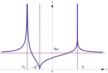
Figure 7: The function $r\equiv r(r_{*})$ defined in Eq.(3.54) for $1<s<\frac{d-1}{d-2}$.

On the other hand, from Eqs.(III) and (3.12) we find

$$\frac{df}{f} = \left[\frac{d-1+z-zr_{s}}{2(d-1)\left(r_{*}-r_{s}\right)}+\frac{d-1+z+zr_{s}}{2(d-1)\left(r_{*}+r_{s}\right)}\right.$$ (3.56)

$$\left.+\frac{1-d-z}{(d-1)\left(r_{*}+r_{s}^{2}\right)}\right]dr_{*},$$

which has the general solution,

$$f=f_{0}\left|r_{*}-r_{s}\right|^{\delta_{1}}\left|r_{*}+r_{s}\right|^{\delta_{2}}\left|r_{*}+r_{s}^{2}\right|^{-\frac{d-1+z}{d-1}},~{}~{}~{}~{}$$ (3.57)

where $f_{0}$ is another integration constant, and

$$\delta_{1}\equiv\frac{d-1+z-zr_{s}}{2(d-1)},\;\;\;\delta_{2}\equiv\frac{d-1+z+zr_{s}}{2(d-1)}.$$ (3.58)

Finally, from Eq.(3.11) we find

$$g^{2}(r_{*})=C_{1}r^{2d}\left(r_{s}^{2}-r_{*}^{2}\right),$$ (3.59)

where $C_{1}\equiv-2d^{2}{g_{e}^{2}\gamma_{1}^{2}}/{(q^{2}\beta)}$. Since $\beta<0$, we find that $C_{1}$ is always positive, $C_{1}>0$. Then, to have $g^{2}$ positive, we must restrict ourselves to the region $|r_{*}|<r_{s}$. Hence, the corresponding metric takes the form,

$$ds^{2}=-N^{2}dt^{2}+G^{2}dr^{2}+\delta_{ij}r^{2}dx^{i}dx^{j},$$ (3.60)

where

$$N^{2} = N_{0}^{2}\frac{r_{s}^{2}-r_{*}^{2}}{\left(r_{*}+r_{s}^{2}\right)^{2}},$$

$$G^{2} = C_{1}r^{2(d-1)}\left(r_{s}^{2}-r_{*}^{2}\right),$$ (3.61)

where $N_{0}\equiv r_{EH}^{z}f_{0}$. The corresponding Ricci scalar is given by

$$R = R_{0}\frac{(r_{*}-r_{s})^{\frac{1-dr_{s}}{d-1}}(r_{*}+r_{s})^{\frac{1+dr_{s}}{d-1}}}{(r_{*}+r_{s}^{2})^{\frac{2d}{d-1}}}$$ (3.62)

$$\times\left[r_{s}^{4}+2r_{*}^{2}+r_{s}^{2}(2r_{*}-1)\right],$$

where

$$R_{0} \equiv \frac{d(d-1)}{r_{EH}^{2d}C_{1}(1-r_{s}^{2})r_{s}^{2}}.$$ (3.63)

Thus, the space-time is always singular at $r_{*}=-r_{s}^{2}$, which divides the regions $|r_{*}|<r_{s}$ into two, $-r_{s}<r_{*}<-r_{s}^{2}$ and $-r_{s}^{2}<r_{*}<r_{s}$.

In the region $-r_{s}<r_{*}<-r_{s}^{2}$, we have $r\in(0,\infty)$. So, in this region the space-time is already complete with a naked singularity located at $r_{*}=-r_{s}^{2}$ (or $r=0$). As $r_{*}\rightarrow-r_{s}^{-}$ or $r\rightarrow\infty$, we find that the metric (3.60) takes the asymptotical form,

$$ds^{2} \simeq L^{2}\bar{r}^{-\frac{2(d-\theta)}{d}}\left(-\bar{r}^{-2(z-1)}d\bar{t}^{2}+d\bar{r}^{2}+\delta_{ij}dx^{i}dx^{j}\right),$$

with

$$\theta=\frac{d(1+dr_{s})}{(d-1)r_{s}},\;\;\;z=\frac{d(1+r_{s})}{(d-1)r_{s}}.$$ (3.65)

The above metric represents Lifshitz space-times with hyperscaling violation.

In the region $-r_{s}^{2}<r_{*}<r_{s}$, the space-time is also singular at $r_{*}=r_{s}$ when $r_{s}>\frac{1}{d}$. Then, the physical interpretation is unclear, as the space-time is singular at both $r=0$ and $r=\infty$. However, when $r_{s}\leq\frac{1}{d}$, the space-time is free of this kind of singularity. In fact, the space-time also take asymptotically the form (3.52) but now with

$$\theta=\frac{d(dr_{s}-1)}{(d-1)r_{s}},\;\;\;z=-\frac{d(1-r_{s})}{(d-1)r_{s}}.$$ (3.66)

IV Universal Horizons and static charged black holes

According to the definition of the universal horizons given in Section II, they can exist only inside the Killing horizons. Then, from the charged solutions presented in the last section, one can see that this is the case only for the solutions given by Eqs.(3.24) and (3.32), for which we have $(\beta,\lambda)=(0,1)$ . Moreover, in order to keep $t$ being asymptotically timelike, in the following we shall consider only the case that the solutions given by Eqs.(3.24) and (3.32) are asymptotically anti-de Sitter, that is,

$$F(r)\simeq\left(\frac{r}{\ell_{d}}\right)^{2},$$ (4.1)

as $r\rightarrow\infty$.

To solve the khronon equation (2.12) in general case is found to be very difficult. But, when $c_{1}+c_{4}=0$, Eq.(2.12) has a simple solution $u^{r}=r_{B}/r^{d}$, where $r_{B}$ is an integration constant. Then, from the condition $u_{\lambda}u^{\lambda}=-1$ we can find $u^{t}$, so finally we have,

$$u^{\mu}=\delta^{\mu}_{t}\frac{\sqrt{r_{B}^{2}+r^{2d}F(r)}}{r^{d}F(r)}-\delta^{\mu}_{r}\frac{r_{B}}{r^{d}}.$$ (4.2)

Hence, we arrive at

$$u_{\mu}\zeta^{\mu} = -\frac{\sqrt{r_{B}^{2}+r^{2d}F(r)}}{r^{d}}.$$ (4.3)

To assure that the four-velocity of the khronon is well-defined in the whole space-time, especially inside the universal horizon, we require that BBM

$$\left.\frac{d}{dr}\left(u_{\mu}\zeta^{\mu}\right)^{2}\right|_{r=r_{UH}}=0,$$ (4.4)

on the universal horizon. Then, from Eq.(4.3) we find that

$$r_{B}^{2}=-F(r_{UH})r_{UH}^{2d},$$ (4.6)

$$2dF(r_{UH})+r_{UH}F^{\prime}(r_{UH})=0.$$

The corresponding surface gravity CLMV is given by,

$$\kappa_{UH} \equiv \frac{1}{2}u^{\alpha}D_{\alpha}\left(u_{\lambda}\zeta^{\lambda}\right)$$ (4.7)

$$= \left.\frac{r_{B}}{2\sqrt{2}r^{d}}\sqrt{G^{\prime\prime}\left(r\right)}\right|_{r=r_{UH}},$$

where

$$G(r)\equiv\frac{r_{B}^{2}}{r^{2d}}+F(r).$$ (4.8)

To study the universal horizons further, we need to consider the cases $d\geq 2$ and $d=1$, separately.

IV.0.1 $d\geq 2$

In this case, from Eq.(4.6) we find that

$$r_{B}^{2}=-Q^{2}r_{UH}^{2}+2mr_{UH}^{1+d}+\frac{2\Lambda_{e}r_{UH}^{2+2d}}{d+d^{2}},$$ (4.9)

where $r_{UH}$ is a real and positive root of Eq.(4.6), which now takes the form,

$$2\left|\Lambda_{e}\right|r_{UH}^{d+1}+dQ^{2}r_{UH}^{1-d}-d(d+1)m=0.$$ (4.10)

Note that in writing the above equation we assumed $\Lambda_{e}<0$ in order for the solutions to be asymptotically anti-de Sitter.

In Figs. 8 and 9, we show the locations of the universal horizons vs the total charge $Q$ for $\Lambda_{e}=-\frac{d(d+1)}{2},\;m=\frac{1}{2}$ in the cases $d=2$ and $d=3$. From these figures we can see that the universal horizons are always inside the outer Killing horizon $r=r_{+}$ but outside the inner horizon $r=r_{-}$. At the extremal case, the universal horizon coincides with two Killing horizons, where the charge of black hole is given by

$$Q_{c}^{2}=-2^{\frac{1-d}{1+d}}\frac{\Lambda_{e}}{d(d-1)}\left[\frac{-\Lambda_{e}}{M(d^{2}-1)}\right]^{-\frac{2d}{d+1}}.$$ (4.11)

When $Q^{2}>Q_{c}^{2}$, the singularity located at the center $r=0$ becomes naked, and no black hole exists. On the other hand, from Figs. 10 and 11 we can see that the surface gravity on the universal horizons are always larger than those on the outer Killing horizons.

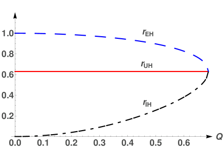
Figure 8: The locations of the universal horizon $r=r_{UH}$, Killing (event) horizon $r=r_{EH}$, and inner horizon $r=r_{IH}$ for the solutions given by Eqs.(3.24) and (3.25) with $d=2,\;\Lambda_{e}=-\frac{d(d+1)}{2},\;m=\frac{1}{2}$.

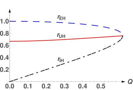
Figure 9: The locations of the universal horizon $r=r_{UH}$, Killing (event) horizon $r=r_{EH}$ and inner horizon $r=r_{IH}$ for the solutions given by Eqs.(3.24) and (3.25) with $d=3$, $\Lambda_{e}=-\frac{d(d+1)}{2}$ and $m=\frac{1}{2}$.

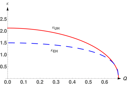
Figure 10: The surface gravity $\kappa_{UH}$ on the universal horizon $r=r_{UH}$, and the one $\kappa_{EH}$ on the event horizon $r=r_{EH}$ for the solutions given by Eqs.(3.24) and (3.25) with $d=2,\;\Lambda_{e}=-\frac{d(d+1)}{2},\;m=\frac{1}{2}$.

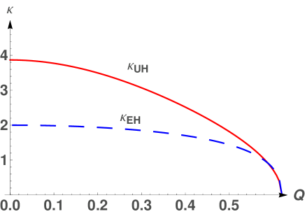
Figure 11: The surface gravity $\kappa_{UH}$ on the universal horizon $r=r_{UH}$, and the one $\kappa_{EH}$ on the event horizon $r=r_{EH}$ for the solutions given by Eqs.(3.24) and (3.25) with $d=3$, $\Lambda_{e}=-\frac{d(d+1)}{2}$ and $m=\frac{1}{2}$.

IV.0.2 $d=1$

In this case the solutions are given by Eqs.(3.32) and (3.33). Substituting $r_{B}$ given by Eq.(4.6) into Eq.(4.6) we find that

$$4Br_{UH}^{2}+2A\ln(r_{UH})+(A-2M)=0.$$ (4.12)

As shown in the last section, depending on the choice of the free parameter $B[=\Lambda/\gamma_{1}]$, the corresponding solutions have different properties.

When $B>0$, it is found that the locations of the universal horizons are different depending on whether $M>B,M=B$ or $M<B$. In particular, when $M>B$, Fig.12 shows the locations of the universal, Killing and inner horizons with different values of $A$, while Fig.13 shows the surface gravity $\kappa_{UH}$ on the universal horizon and $\kappa_{EH}$ on the event horizon $r=r_{EH}$. On the other hand, Figs.14 and 15 are for $M=B$, and Figs.16 and 17 for $M<B$. Again, from these figures we can see that the universal horizons are always inside the outer Killing horizon and outside the inner Killing horizon. However, unlike the previous cases, now the surface gravity at $r=r_{UH}$ can be either larger or smaller than that at $r=r_{EH}$.

It should be noted that for $B>0$ there exist two Killing horizons only when $A\leq 0$. Then, similar to the case $d\geq 2$, the universal horizon coincides with the two Killing horizons in the extremal case, where the three horizons coincide. At this point, the parameter $A$ takes its extremal value $A_{c}$, given by,

$$A_{c}\ln\left(\sqrt{\frac{-A_{c}}{2B}}\right)-\frac{A_{c}}{2}-M=0.$$ (4.13)

In particular, when $M=B$, the above equation yields $A_{c}=-2M$.

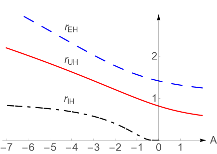
Figure 12: The locations of the universal horizon $r=r_{UH}$, Killing (event) horizon $r=r_{EH}$, and inner horizon $r=r_{IH}$ for the solutions given by Eqs.(3.32) and (3.33) for $M>B>0$. When drawing this figure, we set $(M,B)=(2,1)$.

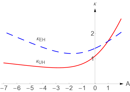
Figure 13: The surface gravity $\kappa_{UH}$ on the universal horizon $r=r_{UH}$, and the surface gravity $\kappa_{EH}$ on the event horizon $r=r_{EH}$ for the solutions given by Eqs.(3.32) and (3.33) for $M>B>0$. When drawing this figure, we set $(M,B)=(2,1)$.

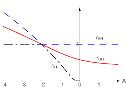
Figure 14: The locations of the universal horizon $r=r_{UH}$, Killing (event) horizon $r=r_{EH}$, and inner horizon $r=r_{IH}$ for the solutions given by Eqs.(3.32) and (3.33) for $M=B>0$. When drawing this figure, we set $(M,B)=(1,1)$.

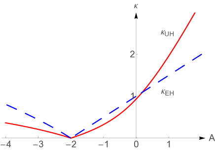
Figure 15: The surface gravity $\kappa_{UH}$ on the universal horizon $r=r_{UH}$, and the surface gravity $\kappa_{EH}$ on the event horizon $r=r_{EH}$ for the solutions given by Eqs.(3.32) and (3.33) for $M=B>0$. When drawing this figure, we set $(M,B)=(1,1)$.

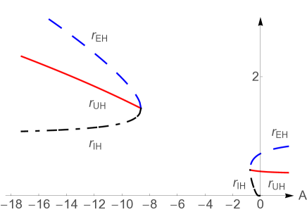
Figure 16: The locations of the universal horizon $r=r_{UH}$, Killing (event) horizon $r=r_{EH}$, and inner horizon $r=r_{IH}$ for the solutions given by Eqs.(3.32) and (3.33) for $B>M>0$. When drawing this figure, we set $(M,B)=(1,2)$.

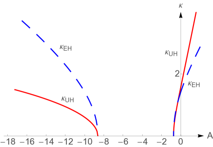
Figure 17: The surface gravity $\kappa_{UH}$ on the universal horizon $r=r_{UH}$, and the surface gravity $\kappa_{EH}$ on the event horizon $r=r_{EH}$ for the solutions given by Eqs.(3.32) and (3.33) for $B>M>0$. When drawing this figure, we set $(M,B)=(1,2)$.

When $B=0$, there exists only one Killing horizon. Fig.18 shows the locations of the universal and Killing horizons with different values of $A$, while Fig.19 shows the surface gravity $\kappa_{UH}$ on the universal horizon and $\kappa_{EH}$ on the event horizon $r=r_{EH}$. It is interesting to note that now the surface gravity on the universal horizon again becomes always larger than that on the outer Killing horizon.

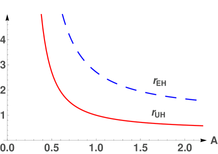
Figure 18: The locations of the universal horizon $r=r_{UH}$ and Killing (event) horizon $r=r_{EH}$ for the solutions given by Eqs.(3.32) and (3.33) for $B=0$. When drawing this figure, we set $M=1$.

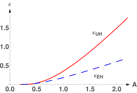
Figure 19: The surface gravity $\kappa_{UH}$ on the universal horizon $r=r_{UH}$, and the surface gravity $\kappa_{EH}$ on the event horizon $r=r_{EH}$ for the solutions given by Eqs.(3.32) and (3.33) for $B=0$. When drawing this figure, we set $M=1$.

When $B<0$, the corresponding solutions are asymptotically de Sitter, and the Killing vector $\zeta^{\mu}=\delta^{\mu}_{t}$ becomes spacelike, $\zeta^{\lambda}\zeta_{\lambda}=-F(r)\rightarrow\infty$, as $r\rightarrow\infty$. Then, it is not clear how to impose the boundary condition for the khronon at $r=\infty$.

V Conclusions

In this paper, we have considered the definition of the universal horizons in any gravitational theories that violate the Lorentz symmetry, first discovered in the study of the black hole thermodynamics in the khronometric theory BS11 . The latter is equivalent to the Einstein-aether theory with the hypersurface-orthogonal condition Jacobson10 . We have found that such a generalization is straightforward, and can be realized by simply promoting the khronon field to a probe field, and has no effects on a given background, quite similar to a Killing field. This is in contrast to all the studies of the universal horizons carried out so far, as in all these studies the khronon was always considered as part of the gravitational field UHsA ; UHsB ; BBM ; CLMV ; SVV , although in some cases its backreactions were assumed to be negligible BS11 .

To apply the definition of the universal horizons to theory with Lorentz violation, we have first studied static charged spacwetimes in the non-projectable HL gravity in the IR limit in Sec. III, and found various solutions. Some of them represent Lifshitz space-times with hyperscaling violation, and some have structures with the presence of Killing horizons. In Sec. IV, we have solved the khronon equation in the space-times that have Killing horizons, and found that universal horizons always exist inside these Killing horizons. Then, the regions inside these universal horizons naturally define black holes in the HL gravity. We have also calculated the surface gravity on these universal horizons, by using the new definition given in CLMV , which seems to be consistent with the first law of black hole mechanics. We have shown explicitly that it can be either larger or smaller than the surface gravity on the Killing horizons, depending on the particular space-time backgrounds considered. It would be very interesting to study the laws of black hole mechanics on the universal horizons found above. Specially what is the role that the charge shall play, and how to define the entropy of these black holes?

In addition, from the definition of the universal horizons one can see that the locations of them usually depend on three free parameters out of the four, $c_{1},...,c_{4}$. When the khronon is part of the gravitational field, each of them has its physical interpretations EA . What are their physical interpretations when the khronon is considered as a probe field? We wish to return to these important issues soon.

Finally, we would like to note that, although in our current paper we have considered black holes only in the IR limit of the non-projectable HL theory BPS , such defined black holes also exist in the full theory of the HL gravity. To see this, let us return to the Schwarzschild black hole given by Eq.(2.1). Blas and Sibiryakov showed that a universal horizon always exist in such a background BS11 . Since the universal horizon is defined in the covariant form (2.2), if it exists in the ($v,r$)-coordinates, it must also exist in the Painleve-Gullstrand coordinates. The Schwarzschild solution given by Eq.(2.18) in the Painleve-Gullstrand coordinates is a solution of the HL gravity not only in the IR limit, but also in the full theory of the HL gravity GLLSW . This is simply because the Ricci tensor $R_{ij}$ of the surfaces $t=$ Constant in these coordinates vanishes identically, so all high-order operators made of $R_{ij}$ have no contributions. Therefore, if it is a solution in the IR limit, it must be also a solution of the full theory. Then, the universal horizon found in the IR limit in BS11 is also the universal horizon of the full theory.

Appendix A: Field Equations of the non-projectable HL Gravity in $(D+1)$-dimensions

In this Appendix, we shall first give a brief introduction to the non-projectable HL theory in $(D+1)$-dimensions, and then consider the constraints from stability and ghost-free conditions. To these goals, let us start with the ADM variables,

$$\left(N,N_{i},g_{ij}\right),\;(i,\;j=1,2,\cdot\cdot\cdot,d+1),$$ (A.1)

which are all functions of both $t$ and $x^{i}$, where $D=d+1$. Then, the general action of the HL theory without the projectability condition in $(D+1)$-dimensional spacetimes is given by

$$S = \zeta^{2}\int dtd^{D+1}xN\sqrt{g}\Big{(}{\cal{L}}_{K}-{\cal{L}}_{{V}}+{\zeta^{-2}}{\cal{L}}_{M}\Big{)},~{}~{}~{}~{}$$ (A.2)

where $g={\rm det}(g_{ij})$, $\zeta^{2}={1}/{(16\pi G)}$, and

$${\cal{L}}_{K}=K_{ij}K^{ij}-\lambda K^{2},$$

$$K_{ij}=\frac{1}{2N}\left(-\dot{g}_{ij}+\nabla_{i}N_{j}+\nabla_{j}N_{i}\right),$$ (A.3)

where $\lambda$ is a dimensionless coupling constant. ${\cal{L}}_{{M}}$ is the Lagrangian of the electromagnetic field, which is given by KM ; KKb

$${\cal{L}}_{M} = \frac{\zeta^{2}}{4g_{e}^{2}}\Big{[}2\frac{g^{ij}}{N^{2}}\left({\cal F}_{0i}-N^{k}{\cal F}_{ki}\right)\left({\cal F}_{0j}-N^{l}{\cal F}_{lj}\right)$$ (A.4)

$$-{\cal F}^{ij}{\cal F}_{ij}-{\cal G}\Big{]},$$

where $g_{e}$ is a coupling constant, $B^{i}=\frac{1}{2}\frac{\epsilon^{ijk}}{\sqrt{g}}{\cal F}_{jk}$, $\epsilon^{ijk}$ is the Levi-Civita symbol, ${\cal F}_{ij}\equiv\nabla_{i}A_{j}-\nabla_{j}A_{i}$, ${\cal F}_{0i}\equiv\partial_{t}A_{i}-\partial_{i}A_{0}$ and the potential of the electromagnetic field is

$${\cal G}=\alpha_{0}+\alpha_{1}B_{i}B^{i}+\alpha_{2}a_{i}B^{i}+{{\cal{G}}}^{z>1},$$ (A.5)

where $\alpha_{i}$ is the arbitrary function of $A^{i}A_{i}$, and ${{\cal{G}}}^{z>1}$ includes all of the operators of ${\cal G}$ higher than order two.

The potential ${\cal{L}}_{V}$ can be cast in the form BPS ; Horava ; ZWWS ,

$${\cal{L}}_{V} = \gamma_{0}\zeta^{2}+\beta a_{i}a^{i}+\gamma_{1}R+{{\cal{L}}}_{V}^{z>1},$$ (A.6)

where $\beta\equiv-\beta_{0}$, and ${{\cal{L}}}_{V}^{z>1}$ includes all of the higher-order derivative terms of ${\cal{L}}_{V}$, and

$$a_{i} = \frac{N_{,i}}{N},\;\;\;a_{ij}=\nabla_{i}a_{j}.$$ (A.7)

V.1 Field Equations

Variation of the action (A.2) with respect to the lapse function $N$ yields the Hamiltonian constraint

$${\cal{L}}_{K}+{\cal{L}}_{V}^{R}+F_{V}=8\pi GJ^{t},\;\;$$ (A.8)

where

$$J^{t} = -\frac{\zeta^{2}}{8g_{e}^{2}}\Big{[}\frac{2g^{ij}}{N^{2}}\left({\cal F}_{0i}-N^{k}{\cal F}_{ki}\right)\left({\cal F}_{0j}-N^{l}{\cal F}_{lj}\right)+{\cal G}$$ (A.9)

$$+{\cal F}^{ij}{\cal F}_{ij}-\alpha_{2}a_{i}B^{i}-\nabla_{i}\left(\alpha_{2}B^{i}\right)]+{J}^{t}_{z>1},$$

$${\cal{L}}_{V}^{R} = \gamma_{0}\zeta^{2}+\gamma_{1}R+{{\cal{L}}}_{V}^{R,z>1},$$ (A.10)

$$F_{V} = -\beta\left(2a^{i}_{i}+a_{i}a^{i}\right)+{F}^{z>1}_{V},$$ (A.11)

where ${{\cal{L}}}_{V}^{R,z>1}$, ${F}_{V}^{z>1}$ and ${J}^{t}_{z>1}$ are all made of spatial derivative terms higher than order 2.

Variation with respect to the shift vector $N_{i}$ yields the momentum constraint

$$\nabla_{j}\pi^{ij}=8\pi GJ^{i},$$ (A.12)

where

$$\pi^{ij} \equiv -K^{ij}+\lambda Kg^{ij},$$

$$J^{i} = \frac{\zeta^{2}g^{lj}}{2g_{e}^{2}N}\left({\cal F}_{0l}-N^{k}{\cal F}_{kl}\right){\cal F}_{ij}+{J}^{i}_{z>1}.$$ (A.13)

Similarly, ${J}^{i}_{z>1}$ consists of spatial derivative terms higher than order 2.

The dynamical equations are obtained by varying with respect to $g_{ij}$,

$$\frac{1}{\sqrt{g}N}\frac{\partial}{\partial t}\left(\sqrt{g}\pi^{ij}\right)+2(K^{ik}K^{j}_{k}-\lambda KK^{ij})$$

$$-\frac{1}{2}g_{ij}{\cal{L}}_{K}+\frac{1}{N}\nabla_{k}(\pi^{ik}N^{j}+\pi^{kj}N^{i}-\pi^{ij}N^{k})$$

$$-F^{ij}-F^{ij}_{a}=8\pi G\tau^{ij},\;\;\;\;\;\;$$ (A.14)

where

$$\tau_{ij} = -\frac{\zeta^{2}}{8g_{e}^{2}}\Big{\{}\frac{2}{N^{2}}\left({\cal F}_{0i}-N^{k}{\cal F}_{ki}\right)\left({\cal F}_{0j}-N^{l}{\cal F}_{lj}\right)$$

$$-2g^{lk}{\cal F}_{il}{\cal F}_{jk}-{\cal G}_{i}j-\frac{g_{ij}}{2}\Big{[}\frac{2}{N^{2}}g^{qp}\left({\cal F}_{0q}-N^{k}{\cal F}_{kq}\right)$$

$$\times\left({\cal F}_{0p}-N^{l}{\cal F}_{lp}\right)-{\cal F}^{lk}{\cal F}_{lk}-{\cal G}\Big{]}\Big{\}}+\tau_{ij}^{z>1},$$

$${\cal G}_{ij} = (\alpha_{0}^{\prime}+\alpha_{1}^{\prime}B_{i}B^{i}+\alpha_{2}^{\prime}a_{i}B^{i})A_{i}A_{j}$$

$$+\alpha_{1}B_{i}B_{j}+\alpha_{2}a_{(i}B_{j)},$$

$$\alpha_{i}^{\prime} = \frac{\partial\alpha_{i}}{\partial(A_{i}A^{i})},$$

$$F^{ij} \equiv \frac{1}{\sqrt{g}N}\frac{\delta(-\sqrt{g}N{\cal{L}}_{V}^{R})}{\delta g_{ij}}$$

$$= -\Lambda g^{ij}+\gamma_{1}\left(R^{ij}-\frac{1}{2}Rg^{ij}\right)$$

$$+\frac{\gamma_{1}}{N}\left(g^{ij}\nabla^{2}N-\nabla^{i}\nabla^{j}N\right)+{F}^{ij}_{z>1},$$

$$F^{ij}_{a} \equiv \frac{1}{\sqrt{g}N}\frac{\delta(-\sqrt{g}N{\cal{L}}_{V}^{a})}{\delta g_{ij}}$$ (A.15)

$$= \beta\left(a^{i}a^{j}-\frac{1}{2}g^{ij}a^{k}a_{k}\right)+{F}^{ij}_{a,z>1},$$

with ${F}^{ij}_{z>1}$, ${F}^{ij}_{a,z>1}$ and $\tau_{ij}^{z>1}$ all made of operators higher than order two of $F^{ij}$, $F^{ij}_{a}$ and $\tau_{ij}$, respectively.

Finally, the Maxwell equations are

$$\nabla^{i}\left[\frac{1}{N}\left({\cal F}_{0i}-N^{k}{\cal F}_{ki}\right)\right]+{\cal E}^{z>1}=0,$$ (A.16)

$$\partial_{t}\left[\frac{g^{ij}}{N}\left({\cal F}_{0j}-N^{k}{\cal F}_{kj}\right)\right]$$

$$-\nabla_{k}\left[\frac{g^{ij}N^{k}-g^{kj}N^{i}}{N}\left({\cal F}_{0j}-N^{l}{\cal F}_{lj}\right)\right]+\nabla_{j}\left(N{\cal F}^{ij}\right)$$

$$-\frac{N}{2}A^{i}(\alpha_{0}^{\prime}+\alpha_{1}^{\prime}B_{l}B^{l}+\alpha_{2}^{\prime}a_{l}B^{l})$$

$$-\frac{\epsilon^{kji}}{4\sqrt{g}}\nabla_{j}\left[N(2\alpha_{1}B_{k}+\alpha_{2}a_{k})\right]+{\cal E}^{i}_{z>1}=0.$$ (A.17)

Again, ${\cal E}^{z>1}$ and ${\cal E}^{i}_{z>1}$ are made of operators higher than order two.

In the infrared (IR) limit, all the quantities made of operators higher than order two can be ignored. This is the case that will be assumed in the rest of the paper.

V.2 Stability and Ghost-free Conditions

When $\gamma_{0}=0$, the above HL theory admits the Minkowski space-time

$$\left(\bar{N},\bar{N}_{i},\bar{g}_{ij}\right)=\left(1,0,\delta_{ij}\right),$$ (A.18)

as a solution of the theory. Then, its linear perturbations reveals that the theory has two modes GHMT , one represents the spin-2 massless gravitons with a dispersion relation,

$$\omega_{T}^{2}=-\gamma_{1}k^{2},$$ (A.19)

and the other represents the spin-0 massless gravitons with

$$\omega_{S}^{2}=-\frac{\gamma_{1}(\lambda-1)}{(d+1)\lambda-1}\left[d\left(\frac{\gamma_{1}}{\beta}-1\right)+1\right]k^{2}.$$ (A.20)

The stability conditions of these modes requires

$$\omega_{T}^{2}>0,\;\;\;\omega_{S}^{2}>0,$$ (A.21)

for any given $k$.

On the other hand, the kinetic term of the spin-0 gravitons is proportional to $(\lambda-1)/[(d+1)\lambda-1]$ GHMT , so the ghost-free condition requires

$$\frac{\lambda-1}{(d+1)\lambda-1}\geq 0.$$ (A.22)

Thus, depending on the values of $d$ and $\lambda$, the stability and ghost-free conditions take different forms.

V.2.1 $\lambda\not=1,\;d\geq 2$

In this case, the conditions (A.21) and (A.22) require

$$\gamma_{1}<0,\;\;\;\frac{d\gamma_{1}}{d-1}<\beta<0,$$ (A.23)

$$i)\;\lambda>1,\;\;\;{\mbox{or}}\;\;\;\;ii)\;\lambda\leq\frac{1}{d+1}.$$ (A.24)

V.2.2 $\lambda=1,\;d\geq 2$

When $\lambda=1$ and $d\geq 2$, we have $\omega_{S}^{2}=0$, and the conditions (A.21) and (A.22) require

$$\gamma_{1}<0,\;\;\;{\mbox{and}}\;\;\beta\;\;{\mbox{is free}}.$$ (A.25)

In particular, $\beta$ can be zero, as can be seen from Eq.(A.20).

V.2.3 $\lambda\not=1,\;d=1$

In this case, the spin-2 gravitons do not exist, as noted above, and then we find that

$$\omega_{S}^{2}=-\frac{\gamma_{1}^{2}(\lambda-1)}{\beta(2\lambda-1)}k^{2}.$$ (A.26)

Thus, the stability and ghost-free conditions require

$$\beta<0,\;\;\;\gamma_{1}\;\;{\mbox{is free}},$$ (A.27)

$$i)\;\lambda>1,\;\;\;{\mbox{or}}\;\;\;\;ii)\;\lambda\leq\frac{1}{2}.$$ (A.28)

V.2.4 $\lambda=1=d$

In this case, from the above we can see that both $\beta$ and $\gamma_{1}$ are free,

$$\beta\;\;{\mbox{and }}\;\;\gamma_{1}\;\;{\mbox{ are all free}}.$$ (A.29)

References

- (1) S. Liberati, Class. Qnatum Grav. 30, 133001 (2013).
- (2) D. Mattingly, Living Rev. Relativity, 8, 5 (2005); S. Liberati and L. Maccione, Annu. Rev. Nucl. Part. Sci. 59, 245 (2009); J. Polchinski, Classical Quantum Gravity 29, 088001 (2012).
- (3) N. Arkani-Hamed, H.C. Cheng, M.A. Luty, and S. Mukohyama, J. High Energy Phys. 05, 074 (2004).
- (4) T. Jacobson and Mattingly, Phys. Rev. D64, 024028 (2001); T. Jacobson, Proc. Sci. QG-PH, 020 (2007) [arXiv:0801.1547].
- (5) P. Hořava, Phys. Rev. D79, 084008 (2009).
- (6) S. Mukohyama, Class. Quantum Grav. 27, 223101 (2010); P. Hořava, Class. Quantum Grav. 28, 114012 (2011); T. Clifton, P.G. Ferreira, A. Padilla, and C. Skordis, Phys. Rept. 513, 1 (2012).
- (7) K. Lin, S. Mukohyama, A. Wang, and T. Zhu, Phys. Rev. D89, 084022 (2014).
- (8) K. Yagi, D. Blas, E. Barausse, and N. Yunes, Phys. Rev. D89, 084067 (2014); K. Yagi, D. Blas, N. Yunes, and E. Barausse, Phys. Rev. Lett. 112, 161101 (2014).
- (9) S. Mukohyama, JCAP 0906, 001 (2009); A. Wang and R. Maartens, Phys. Rev. D81, 024009 (2010); A. Wang, D. Wands, and R. Maartens, J. Cosmol. Astropart. Phys., 03, 013 (2010); J.-O. Gong, S. Koh, and M. Sasaki, Phys. Rev. D81, 084053 (2010); A. Wang, Phys. Rev. D82, 124063 (2010).
- (10) X. Gao, Y. Wang, R. Brandenberger, and A. Riotto, Phys. Rev. D81, 083508 (2010); B. Chen, S. Pi and J. -Z. Tang, JCAP 0908, 007 (2009); T. Kobayashi, Y. Urakawa, and M. Yamaguchi, JCAP, 04, 025 (2010); A. Cerioni and R. H. Brandenberger, arXiv:1008.3589; R.-G. Cai, B. Hu, and H.-B. Zhang, Phys. Rev. D83, 084009 (2011).
- (11) Y.-Q. Huang, A. Wang, and Q. Wu, JCAP, 10, 010 (2012); Y.-Q. Huang and A. Wang, Phys. Rev. D86, 103523 (2012).
- (12) T. Zhu, Y.-Q. Huang, and A. Wang, JHEP, 01, 138 (2013); A. Wang, Q. Wu, W. Zhao, and T. Zhu, Phys. Rev. D87, 103512 (2013); T. Zhu, W. Zhao, Y.-Q. Huang, A. Wang, and Q. Wu, Phys. Rev. D88, 063508 (2013).
- (13) E. Kiritsis and G. Kofinas, JHEP 01, 122 (2010); D. Capasso and A.P. Polychronakos, ibid., 02, 068 (2010).
- (14) J. Greenwald, J. Lenells, J. X. Lu, V. H. Satheeshkumar, and A. Wang, Phys. Rev. D84, 084040 (2011); A. Wang, Phys. Rev. Lett. 110, 091101 (2013).
- (15) J.W. Elliott, G.D. Moore, and H. Stoica, JHEP 08, 066 (2005).
- (16) D. Blas and S. Sibiryakov, Phys. Rev. D84, 124043 (2011).
- (17) E. Barausse, T. Jacobson, and T. Sotiriou, Phys. Rev. D83, 124043 (2011); B. Cropp, S. Liberati, and M. Visser, Class. Quantum Grav. 30, 125001 (2013); S. Janiszewski, arXiv:1401.1463; S. Janiszewski, A. Karch, B. Robinson, and D. Sommer, JHEP 04, 163 (2014).
- (18) M. Saravani, N. Afshordi, and R.B. Mann, Phys. Rev. D89, 084029 (2014); A. Mohd, arXiv:1309.0907; C. Eling and Y. Oz, arXiv:1408.0268.
- (19) P. Berglund, J. Bhattacharyya, and D. Mattingly, Phys. Rev. D85, 124019 (2012); Phys. Rev. Lett. 110, 071301 (2013).
- (20) B. Cropp, S. Liberati, A. Mohd, and M. Visser, Phys. Rev. D89, 064061 (2014).
- (21) T. Sotiriou, I. Vega, and D. Vernieri, arXiv:1405.3715.
- (22) D. Blas, O. Pujolas, and S. Sibiryakov, Phys. Lett. B688, 350 (2010); J. High Energy Phys. 1104, 018 (2011).
- (23) T. Jacobson, Phys. Rev. D81, 101502 (R) (2010).
- (24) A. Wang, On “No-go theorem for slowly rotating black holes in Hořava-Lifshitz gravity, arXiv:1212.1040.
- (25) R.-G. Cai, L.-M. Cao and N. Ohta, Phys. Rev. D80 (2009) 024003; S.-S. Kim, T. Kim and Y. Kim, Phys. Rev. D80 (2009) 124002; E. O Colgain and H. Yavartanoo, JHEP 08 (2009) 021; J.-Z. Tang, arXiv:0911.3849; E. Gruss, Class. Quant. Grav. 28 (2011) 085007; J.M. Romero, J.A. Santiago, O. Gonzalez-Gaxiola and A. Zamora, Mod. Phys. Lett. A25 (2010) 3381; A. Borzou, K. Lina, and A. Wang, JCAP 02 (2012) 025.
- (26) S. Maeda, S. Mukohyama and T. Shiromizu, Phys. Rev. D80 (2009) 123538.
- (27) S.W. Hawking and G.F.R. Ellis, The large scale structure of space-time, Cambridge Monographs on Mathematical Physics, (Cambridge University Press, Cambridge, 1973).
- (28) F.J. Tipler, Nature, 270, 500 (1977).
- (29) S.A. Hayward, Phys. Rev. D49, 6467 (1994); Class. Quantum Grav. 17, 1749 (2000).
- (30) A. Wang, Phys. Rev. D68, 064006 (2003); ibid., D72, 108501 (2005); Gen. Relativ. Grav. 37, 1919 (2005); A.Y. Miguelote, N.A. Tomimura, and A. Wang, ibid., 36, 1883 (2004); and P. Sharma, A. Tziolas, A. Wang, and Z.-C. Wu, Inter. J. Mord. Phys. A26, 273 (2011).
- (31) P. Horava and C.M. Melby-Thompson, Gen. Relativ. Grav. 43, 1391 (2011).
- (32) T. Suyama, JHEP, 01, 093 (2010); J. Alexandre, K. Farakos, P. Pasipoularides, and A. Tsapalis, Phys. Rev. D81, 045002 (2010); J.M. Romero, V. Cuesta, J.A. Garcia, and J. D. Vergara, ibid., D81, 065013 (2010); S.K. Rama, arXiv:0910.0411; L. Sindoni, arXiv:0910.1329; I. Kimpton and A. Padilla, JHEP 04 (2013) 133. Matter in Horava-Lifshitz gravity Ian Kimpton, Antonio Padilla (Nottingham U.). Jan 2013. 25 pp. Published in JHEP 1304 (2013) 133
- (33) E. Kiritsis and G. Kofinas, Nucl. Phys. B821, (2009) 467.
- (34) R.M. Wald, General Relativity (The University of Chicago Press, Chicago, 1984).
- (35) C. Eling and T. Jacobson, Class. Quantum Grav. 23, 5643 (2006).
- (36) P. Painleve, C. R. Acad. Sci. (Paris) 173, 677 (1921); A. Gullstrand, Arkiv. Mat. Astron. Fys. 16, 1 (1922).
- (37) R.-G. Cai and A. Wang, Phys. Lett. B686, 166 (2010).
- (38) K. Lin, F.-W. Shu, A. Wang, and Q. Wu, arXiv:1404.3413.
- (39) F.-W. Shu, K. Lin, A. Wang, and Q. Wu, J. High Energy Phys. 04 (2014) 056.
- (40) Y. Wu, M. F. A. da Silva, N. O. Santos, and A. Wang, Phys. Rev. D68, 084012 (2003).
- (41) M. Banados, C. Teitelboim, and J. Zanelli, Phys. Rev. Lett. 69, 1849 (1992).
- (42) T. Griffin, P. Hořava, and C. Melby-Thompson, Phys. Rev. Lett. 110, 081602 (2013).
- (43) T. Zhu, Q. Wu, A. Wang, and F.-W. Shu, Phys. Rev. D84, 101502 (R) (2011); T. Zhu, F.-W. Shu, Q. Wu, and A. Wang, Phys. Rev. D85, 044053 (2012); K. Lin, S. Mukohyama, A. Wang, and T. Zhu, arXiv:1310.6666.