A Dichotomy of Functions in Distributed Coding: An Information Spectral Approach

Abstract

The problem of distributed data compression for function computation is considered, where (i) the function to be computed is not necessarily symbol-wise function and (ii) the information source has memory and may not be stationary nor ergodic. We introduce the class of smooth sources and give a sufficient condition on functions so that the achievable rate region for computing coincides with the Slepian-Wolf region (i.e., the rate region for reproducing the entire source) for any smooth sources. Moreover, for symbol-wise functions, the necessary and sufficient condition for the coincidence is established. Our result for the full side-information case is a generalization of the result by Ahlswede and Csiszár to sources with memory; our dichotomy theorem is different from Han and Kobayashi’s dichotomy theorem, which reveals an effect of memory in distributed function computation. All results are given not only for fixed-length coding but also for variable-length coding in a unified manner. Furthermore, for the full side-information case, the error probability in the moderate deviation regime is also investigated.

I Introduction

We study the problem of distributed data compression for function computation described in Fig. 2 and Fig. 2, where the function to be computed is not necessarily symbol-wise function. In [1], Körner and Marton revealed that the achievable rate region for computing modulo-sum is strictly larger than the rate region that can be achieved by first applying Slepian-Wolf coding [2] and then computing the function. Since then, distributed coding schemes that are tailored for some classes of functions were studied (e.g., see [3, Chapter 21]). These results are the cases such that the structure of functions can be utilized for distributed coding. However, not all functions have such nice structures, and even for some classes of functions, it is known that the Slepian-Wolf region cannot be improved at all [4, 5], i.e., reproducing function value is as difficult as reproducing the entire source. Thus, it is important to understand what makes distributed computation difficult, which is the main theme of this paper. This direction of research has been studied for i.i.d. sources, which will be reviewed next.

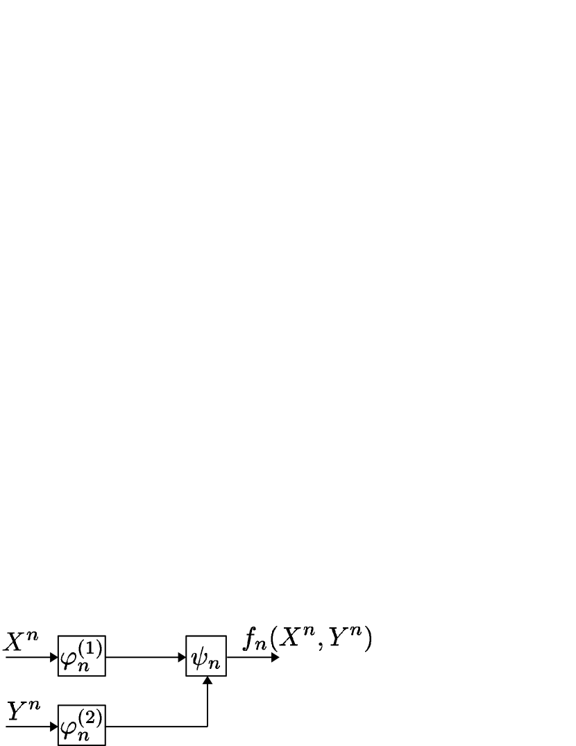
Figure 1: Distributed computing

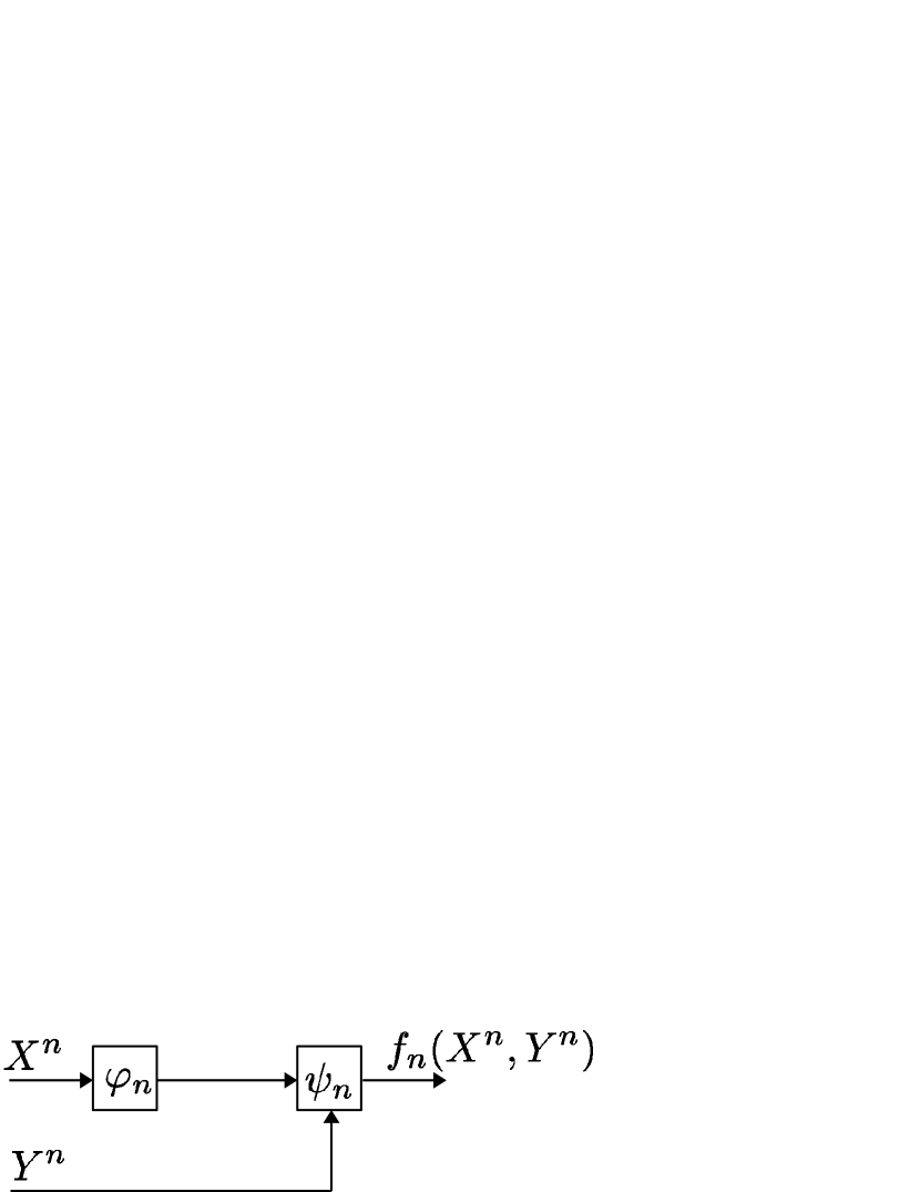
Figure 2: Distributed computing with full-side-information

In [4], Ahlswede and Csiszár investigated distributed coding for function computation when the full side-information is available at the decoder (see Fig. 2); they introduced the concept of sensitive functions, and showed that the achievable rate for computing sensitive functions coincides with the achievable rate of Slepian-Wolf coding (with full side-information) provided that the source is an i.i.d. source satisfying the positivity condition. Surprisingly, the class of sensitive functions includes a function such that the image size is just one bit. Later, El Gamal gave a simple proof of Ahlswede and Csiszár’s result [6].

In [5], Han and Kobayashi investigated distributed coding for function computation with two-encoders case (see Fig. 2); they considered the class of symbol-wise functions, and derived the necessary and sufficient condition of functions such that the achievable rate region coincides with that of Slepian-Wolf coding for any i.i.d. sources satisfying the positivity condition. In the rest of the paper, we shall call functions satisfying Han and Kobayashi’s condition HK functions.

For the class of i.i.d. sources satisfying the positivity condition, the above mentioned two results [4, 5] showed some classes of functions that are difficult to compute via distributed coding. Then, a natural question is:

($\spadesuit$)

Are functions in those classes difficult to compute even for wider classes of sources that have memory and may not be stationary nor ergodic?

In order to answer this question in a unified manner, we study distributed computation problem by information-spectral approach [7, 8]. Our contributions are summarized as follows.

I-A Contributions

First, we introduce a class of sources which we called smooth sources; other than the smooth condition, we do not impose any condition on sources, i.e., we consider general sources. Roughly speaking, the smooth condition says that the probability of a sequence does not change significantly when we flip a symbol of the sequence. When we restrict sources to be i.i.d., then the smooth condition coincides with the positivity condition studied in [4, 5]. However, the class of smooth sources is much wider than the class of i.i.d. sources satisfying the positivity condition. In fact, it includes Markov sources with positive transition matrices or mixtures of i.i.d. sources satisfying positivity condition.

Next, we introduce the concept of joint sensitivity; a function $f_{n}$ is said to be jointly sensitive if $f_{n}(\bm{x},\bm{y})\neq f_{n}(\hat{\bm{x}},\hat{\bm{y}})$ whenever $\bm{x}\neq\hat{\bm{x}}$ and $\bm{y}\neq\hat{\bm{y}}$. Then, we introduce the class of totally sensitive functions as the set of all functions that are sensitive in the sense of [4] and also jointly sensitive. When we restrict functions to be symbol-wise, the class of totally sensitive functions is a strict subset of the class of HK functions. However, totally sensitive functions are not necessarily symbol-wise. The inclusive relation among the classes of functions is summarized in Fig. 3.

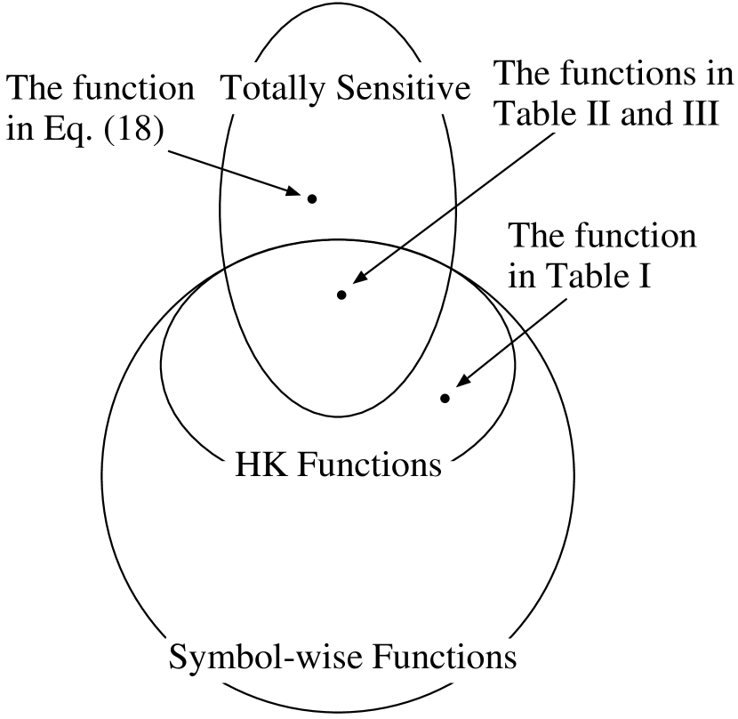
Figure 3: The inclusive relation among the classes of functions.

When the full side-information is available at the decoder, we show that the Slepian-Wolf rate cannot be improved if the function is sensitive and the source is smooth. This result generalizes the result in [4] for smooth sources. Thus, for the class of sensitive functions, the answer to Question ($\spadesuit$) is positive in the sense that the Slepian-Wolf rate cannot be improved.

For the two-encoders case, we show that the Slepian-Wolf region cannot be improved if the function is totally sensitive and the source is smooth. Furthermore, for symbol-wise functions, we show that the achievable region coincides with the Slepian-Wolf region for any smooth sources if and only if the function is totally sensitive. In fact, for a function that satisfies Han and Kobayashi’s condition but is not totally sensitive, there exists a finite state source, which is smooth, such that the Slepian-Wolf region can be improved. This dichotomy theorem can be regarded as a smooth source counterpart of Han and Kobayashi’s dichotomy theorem [5]; we need the condition that is more strict than Han and Kobayashi’s condition because we broaden the class of sources. Consequently, for the class of HK functions, the answer to Question ($\spadesuit$) is negative in the sense that the Slepian-Wolf region can be improved; but we can say that totally sensitive functions are difficult to compute via distributed coding for any smooth sources.

When a function is sensitive but not totally sensitive, the sum rate can be improved in general. To derive an outer bound for such a case, we introduce another class of functions, which we call $r$-totally sensitive. Then, we show that the improvement of sum rate is at most $r$. Furthermore, we also show that there exist a smooth source and an $r$-totally sensitive function such that our outer bound is saturated, which means that our outer bound cannot be improved anymore only from the two assumptions: smooth condition and $r$-total sensitivity.

We also derive the following refinements of the above results. So far, the study of distributed computing has been restricted to the fixed-length coding in the literature [4, 5]. In this paper, by using the techniques developed by the authors in [10], we show that the above mentioned results also hold even for the variable-length coding. Furthermore, for the full side-information case, we show that the Slepian-Wolf rate cannot be improved even in the moderate deviation regime [11, 12].

Although our main contributions of this paper are structural connections between the achievable rate regions (or rates) for function computing and the Slepian-Wolf regions (or rates), as a byproduct, we can derive explicit forms of the achievable regions (or rates) by using the corresponding results on the Slepian-Wolf regions (or rates). It is also known that distributed computing can be regarded as a special case of distributed lossy coding studied by Yamamoto [13] (see also [14]). Thus, our results may be interesting from the view point of distributed lossy coding for smooth sources.

From technical perspective, we elaborate El Gamal’s argument [6] so that it can be used for the wider class of sources; Lemma 1 is the core of the proofs, and it enables us to prove our main results for both fixed-length coding and variable-length coding in a unified manner. The bounds in Lemma 1 is also tight enough to be used for the moderate deviation analysis.

I-B Organization of Paper

In Section II, we introduce the coding problem investigated in this paper, and also introduce classes of functions and classes of sources. Then, in Section III, main coding theorems are stated. The proofs of main results are given in Section IV, where proofs of some lemmas are shown in Appendices.

I-C Notation

Throughout this paper, random variables (e.g., $X$) and their realizations (e.g., $x$) are denoted by capital and lower case letters respectively. All random variables take values in some finite alphabets which are denoted by the respective calligraphic letters (e.g., $\mathcal{X}$). Similarly, $X^{n}\triangleq(X_{1},X_{2},\dots,X_{n})$ and $x^{n}\triangleq(x_{1},x_{2},\dots,x_{n})$ denote, respectively, a random vector and its realization in the $n$th Cartesian product $\mathcal{X}^{n}$ of $\mathcal{X}$. We will use bold lower letters to represent vectors if the length $n$ is apparent from the context; e.g., we use $\bm{x}$ instead of $x^{n}$.

For a finite set $\mathcal{S}$, $\left\lvert\mathcal{S}\right\rvert$ denotes the cardinality of $\mathcal{S}$ and $\mathcal{S}^{*}$ denotes the set of all finite strings drawn from $\mathcal{S}$. For a sequence $\bm{s}\in\mathcal{S}^{*}$, $\left\lvert\bm{s}\right\rvert$ denotes the length of $\bm{s}$. The Hamming distance between two sequences $\bm{s},\hat{\bm{s}}\in\mathcal{S}^{n}$ is defined as $d(\bm{s},\hat{\bm{s}})\triangleq\left\lvert\{i:s_{i}\neq\hat{s}_{i}\}\right\rvert$. $\mathcal{S}^{c}$ denotes the complement of $\mathcal{S}$.

Information-theoretic quantities are denoted in the usual manner [15, 16]. For example, $H(X|Y)$ denotes the conditional entropy of $X$ given $Y$. All logarithms are with respect to base 2.

Moreover, we will use quantities defined by using the information-spectrum method [8]. Here, we recall the probabilistic limit operation: For a sequence $\bm{Z}\triangleq\{Z_{n}\}_{n=1}^{\infty}$ of real-valued random variables, the limit superior in probability of $\bm{Z}$ is defined as

$$\text{p-}\limsup_{n\to\infty}Z_{n} \triangleq\inf\left\{\alpha:\lim_{n\to\infty}\Pr\{Z_{n}>\alpha\}=0\right\}.$$ (1)

II Problem

II-A General Setting

Let $(\bm{X},\bm{Y})=\{(X^{n},Y^{n})\}_{n=1}^{\infty}$ be a general correlated source with finite alphabets $\mathcal{X}$ and $\mathcal{Y}$. We consider a sequence $\bm{f}=\{f_{n}\}_{n=1}^{\infty}$ of functions $f_{n}\colon\mathcal{X}^{n}\times\mathcal{Y}^{n}\to\mathcal{Z}_{n}$. A variable-length code $\Phi$ for computing $f_{n}$ is defined by a triplet $(\varphi_{n}^{(1)},\varphi_{n}^{(2)},\psi_{n})$ of the first encoder $\varphi_{n}^{(1)}\colon\mathcal{X}^{n}\to\{0,1\}^{*}$, the second encoder $\varphi_{n}^{(2)}\colon\mathcal{Y}^{n}\to\{0,1\}^{*}$, and a decoder $\psi_{n}\colon\mathcal{C}_{n}^{(1)}\times\mathcal{C}_{n}^{(2)}\to\mathcal{Z}_{n}$, where $\mathcal{C}_{n}^{(1)}\triangleq\{\varphi_{n}^{(1)}(\bm{x}):\bm{x}\in\mathcal{X}^{n}\}\subseteq\{0,1\}^{*}$ and $\mathcal{C}_{n}^{(2)}\triangleq\{\varphi_{n}^{(2)}(\bm{y}):\bm{y}\in\mathcal{Y}^{n}\}\subseteq\{0,1\}^{*}$. We assume that both of $\mathcal{C}_{n}^{(1)}$ and $\mathcal{C}_{n}^{(2)}$ satisfy the prefix condition.

For each $i=1,2$, $\varphi_{n}^{(i)}$ is said to be a fixed-length encoder if $\mathcal{C}_{n}^{(i)}$ consists of codewords of the same length. A code $\Phi_{n}$ is called a fixed-length code if both of $\varphi_{n}^{(i)}$ ($i=1,2$) are fixed-length encoders. Clearly, the class of all variable-length codes includes that of all fixed-length codes as a strict subclass.

The average codeword length and the error probability of $\Phi_{n}$ are respectively defined as

$$\mathbb{E}\left[\left\lvert\varphi_{n}^{(1)}(X^{n})\right\rvert\right] \triangleq\sum_{\bm{x}}P_{X^{n}}(\bm{x})\left\lvert\varphi_{n}^{(1)}(\bm{x})\right\rvert,$$ (2)

$$\mathbb{E}\left[\left\lvert\varphi_{n}^{(2)}(Y^{n})\right\rvert\right] \triangleq\sum_{\bm{y}}P_{Y^{n}}(\bm{y})\left\lvert\varphi_{n}^{(2)}(\bm{y})\right\rvert,$$ (3)

and

$$\mathrm{P}_{\mathrm{e}}(\Phi_{n}|f_{n}) \triangleq\Pr\left\{f_{n}(X^{n},Y^{n})\neq\psi_{n}\left(\varphi_{n}^{(1)}(X^{n}),\varphi_{n}^{(2)}(Y^{n})\right)\right\}.$$ (4)

Definition 1.

Given a source $(\bm{X},\bm{Y})$ and a sequence of functions $\bm{f}=\{f_{n}\}_{n=1}^{\infty}$, a pair $(R_{1},R_{2})$ of rates is said to be achievable, if there exists a sequence $\{\Phi_{n}\}_{n=1}^{\infty}$ of codes satisfying

$$\lim_{n\to\infty}\mathrm{P}_{\mathrm{e}}(\Phi_{n}|f_{n}) =0$$ (5)

and

$$\limsup_{n\to\infty}\frac{1}{n}\mathbb{E}\left[\left\lvert\varphi_{n}^{(1)}(X^{n})\right\rvert\right] \leq R_{1},$$ (6)

$$\limsup_{n\to\infty}\frac{1}{n}\mathbb{E}\left[\left\lvert\varphi_{n}^{(2)}(Y^{n})\right\rvert\right] \leq R_{2}.$$ (7)

The set of all achievable rate pairs is denoted by $\mathcal{R}^{\mathsf{vl}}(\bm{X},\bm{Y}|\bm{f})$.

Definition 2.

Given a source $(\bm{X},\bm{Y})$ and a sequence of functions $\bm{f}=\{f_{n}\}_{n=1}^{\infty}$, a pair $(R_{1},R_{2})$ of rates is said to be achievable by fixed-length coding, if there exists a sequence $\{\Phi_{n}\}_{n=1}^{\infty}$ of fixed-length codes satisfying (5), (6), and (7). The set of all rate pairs that are achievable by fixed-length coding is denoted by $\mathcal{R}^{\mathsf{fl}}(\bm{X},\bm{Y}|\bm{f})$.

A variable-length (resp. fixed-length) code $\Phi_{n}$ for computing the identity function $f_{n}^{\mathsf{id}}(\bm{x},\bm{y})\triangleq(\bm{x},\bm{y})$ is called a variable-length (resp. fixed-length) Slepian-Wolf (SW) code.

Definition 3 (SW region).

For a source $(\bm{X},\bm{Y})$, the achievable rate region $\mathcal{R}^{\mathsf{vl}}(\bm{X},\bm{Y}|\bm{f}^{\mathsf{id}})$ for $(\bm{X},\bm{Y})$ and the sequence $\bm{f}^{\mathsf{id}}\triangleq\{f_{n}^{\mathsf{id}}\}_{n=1}^{\infty}$ of identity functions is called the Slepian-Wolf (SW) region and denoted by $\mathcal{R}_{\mathsf{SW}}^{\mathsf{vl}}(\bm{X},\bm{Y})$. By considering only fixed-length codes, $\mathcal{R}_{\mathsf{SW}}^{\mathsf{fl}}(\bm{X},\bm{Y})$ is defined similarly.

Remark 1.

From the definitions, it is apparent that $\mathcal{R}_{\mathsf{SW}}^{\mathsf{vl}}(\bm{X},\bm{Y})\subseteq\mathcal{R}^{\mathsf{vl}}(\bm{X},\bm{Y}|\bm{f})$ and $\mathcal{R}_{\mathsf{SW}}^{\mathsf{fl}}(\bm{X},\bm{Y})\subseteq\mathcal{R}^{\mathsf{fl}}(\bm{X},\bm{Y}|\bm{f})$ for any $(\bm{X},\bm{Y})$ and $\bm{f}$.

Remark 2.

A general formula for the SW region for fixed-length coding was given by Miyake and Kanaya [17] as

$$\mathcal{R}_{\mathsf{SW}}^{\mathsf{fl}}(\bm{X},\bm{Y}) =\left\{(R_{1},R_{2}):R_{1}\geq\overline{H}(\bm{X}|\bm{Y}),R_{2}\geq\overline{H}(\bm{Y}|\bm{X}),R_{1}+R_{2}\geq\overline{H}(\bm{X},\bm{Y})\right\}$$ (8)

where

$$\overline{H}(\bm{X},\bm{Y}) \triangleq\text{p-}\limsup_{n\to\infty}\frac{1}{n}\log\frac{1}{P_{X^{n}Y^{n}}(X^{n}Y^{n})},$$ (9)

$$\overline{H}(\bm{X}|\bm{Y}) \triangleq\text{p-}\limsup_{n\to\infty}\frac{1}{n}\log\frac{1}{P_{X^{n}|Y^{n}}(X^{n}|Y^{n})},$$ (10)

$$\overline{H}(\bm{Y}|\bm{X}) \triangleq\text{p-}\limsup_{n\to\infty}\frac{1}{n}\log\frac{1}{P_{Y^{n}|X^{n}}(Y^{n}|X^{n})}.$$ (11)

As long as the authors know, a general formula for $\mathcal{R}_{\mathsf{SW}}^{\mathsf{vl}}(\bm{X},\bm{Y})$ is not known. One of our contributions is to demonstrate that we can discuss the equivalence between $\mathcal{R}_{\mathsf{SW}}^{\mathsf{vl}}(\bm{X},\bm{Y})$ and $\mathcal{R}^{\mathsf{vl}}(\bm{X},\bm{Y}|\bm{f})$ without knowing the precise form of $\mathcal{R}_{\mathsf{SW}}^{\mathsf{vl}}(\bm{X},\bm{Y})$; for specific sources such that the precise form of $\mathcal{R}_{\mathsf{SW}}^{\mathsf{vl}}(\bm{X},\bm{Y})$ is known, we can get the precise form of $\mathcal{R}^{\mathsf{vl}}(\bm{X},\bm{Y}|\bm{f})$ as a byproduct.

As a special case of distributed computation, we are interested in the case where $\bm{y}\in\mathcal{Y}^{n}$ is completely known at the decoder as the side-information. We call this case as the “full-side-information case”. The optimal coding rates which are achievable in full-side-information case are defined as follows.

Definition 4 (SW rate).

For any $(\bm{X},\bm{Y})$ and $\bm{f}$, let

$$R^{\mathsf{vl}}(\bm{X}|\bm{Y}|\bm{f}) \triangleq\inf\left\{R_{1}:(R_{1},\log\left\lvert\mathcal{Y}\right\rvert)\in\mathcal{R}^{\mathsf{vl}}(\bm{X},\bm{Y}|\bm{f})\right\},$$ (12)

$$R^{\mathsf{fl}}(\bm{X}|\bm{Y}|\bm{f}) \triangleq\inf\left\{R_{1}:(R_{1},\log\left\lvert\mathcal{Y}\right\rvert)\in\mathcal{R}^{\mathsf{fl}}(\bm{X},\bm{Y}|\bm{f})\right\}.$$ (13)

Similarly, for any $(\bm{X},\bm{Y})$, let

$$R_{\mathsf{SW}}^{\mathsf{vl}}(\bm{X}|\bm{Y}) \triangleq\inf\left\{R_{1}:(R_{1},\log\left\lvert\mathcal{Y}\right\rvert)\in\mathcal{R}_{\mathsf{SW}}^{\mathsf{vl}}(\bm{X},\bm{Y})\right\},$$ (14)

$$R_{\mathsf{SW}}^{\mathsf{fl}}(\bm{X}|\bm{Y}) \triangleq\inf\left\{R_{1}:(R_{1},\log\left\lvert\mathcal{Y}\right\rvert)\in\mathcal{R}_{\mathsf{SW}}^{\mathsf{fl}}(\bm{X},\bm{Y})\right\}.$$ (15)

Remark 3.

From (8), we have $R_{\mathsf{SW}}^{\mathsf{fl}}(\bm{X}|\bm{Y})=\overline{H}(\bm{X}|\bm{Y})$. A general formula for $R_{\mathsf{SW}}^{\mathsf{vl}}(\bm{X}|\bm{Y})$ is recently given by the authors [10].

II-B Function Classes

In this subsection, we introduce important classes of functions investigated in this paper. First, we state the concept of sensitivity introduced in [4] and related properties.

Definition 5 (Sensitivity).

A function $f_{n}\colon\mathcal{X}^{n}\times\mathcal{Y}^{n}\to\mathcal{Z}_{n}$ is said to be sensitive conditioned on $\mathcal{Y}^{n}$ if it satisfies the following property: If $\bm{x},\hat{\bm{x}},\bm{y}$ satisfy $f_{n}(\bm{x},\bm{y})=f_{n}(\hat{\bm{x}},\bm{y})$ and $x_{i}\neq\hat{x}_{i}$ for some $i$ then there exists $\hat{\bm{y}}\in\mathcal{Y}^{n}$ such that $\hat{y}_{i}\neq y_{i}$, $\hat{y}_{j}=y_{j}$ for any $j\neq i$ and $f_{n}(\bm{x},\hat{\bm{y}})\neq f_{n}(\hat{\bm{x}},\hat{\bm{y}})$.

Similarly, a function $f_{n}\colon\mathcal{X}^{n}\times\mathcal{Y}^{n}\to\mathcal{Z}_{n}$ is said to be sensitive conditioned on $\mathcal{X}^{n}$ if it satisfies the property, where the role of $\bm{x}$ (resp. $\hat{\bm{x}}$) in Definition 5 is switched with that of $\bm{y}$ (resp. $\hat{\bm{y}}$).

Remark 4.

In [6], the concenpt of $\alpha$-sensitive functions, which includes sensitive functions as a special case, is introduced, and it is shown that the result of [4], which is proved for sensitive functions, can be proved also for $\alpha$-sensitive functions. Although our results for sensitive functions hold also for $\alpha$-sensitive functions, we consider only sensitive functions for simplicity.

Now, we introduce some new sensitivity conditions.

Definition 6 (Joint sensitivity).

A function $f_{n}\colon\mathcal{X}^{n}\times\mathcal{Y}^{n}\to\mathcal{Z}_{n}$ is said to be jointly sensitive if $f_{n}(\bm{x},\bm{y})\neq f_{n}(\hat{\bm{x}},\hat{\bm{y}})$ holds for every $\bm{x}\neq\hat{\bm{x}}$ and $\bm{y}\neq\hat{\bm{y}}$.

Definition 7 (Total sensitivity).

A function $f_{n}\colon\mathcal{X}^{n}\times\mathcal{Y}^{n}\to\mathcal{Z}_{n}$ is said to be totally sensitive if it is jointly sensitive and sensitive conditioned on both of $\mathcal{X}^{n}$ and $\mathcal{Y}^{n}$.

Example 1.

Let $P_{\bm{x}\bm{y}}$ be the joint type of $(\bm{x},\bm{y})$ [16]; i.e., $P_{\bm{x}\bm{y}}$ is a joint distribution on $\mathcal{X}\times\mathcal{Y}$ such as

$$P_{\bm{x}\bm{y}}(a,b)\triangleq\frac{\lvert\{i:(x_{i},y_{i})=(a,b)\}\rvert}{n},\quad(a,b)\in\mathcal{X}\times\mathcal{Y}.$$ (16)

The type function $f_{n}(\bm{x},\bm{y})\triangleq P_{\bm{x}\bm{y}}$ is sensitive conditioned on both of $\mathcal{X}^{n}$ and $\mathcal{Y}^{n}$ but is not jointly sensitive. Hence, it is not totally sensitive.

Example 2.

The function defined by

$$f_{n}(\bm{x},\bm{y})\triangleq\left\{\begin{array}[]{ll}(>,\bm{x})&\mbox{if }\bm{x}>\bm{y}\\ (=,\bm{x})&\mbox{if }\bm{x}=\bm{y}\\ (<,\bm{y})&\mbox{if }\bm{x}<\bm{y}\end{array}\right.,$$ (20)

where $>$ and $<$ are with respect to arbitrary ordering on $\mathcal{X}^{n}=\mathcal{Y}^{n}$, is jointly sensitive but is not sensitive conditioned on $\mathcal{X}^{n}$ (nor $\mathcal{Y}^{n}$). On the other hand,

$$f^{\prime}_{n}(\bm{x},\bm{y})\triangleq(P_{\bm{x}\bm{y}},f_{n}(\bm{x},\bm{y}))$$ (21)

is totally sensitive.

Next, we consider special classes of symbol-wise functions. Given a function $f$ on $\mathcal{X}\times\mathcal{Y}$, the function $f_{n}$ on $\mathcal{X}^{n}\times\mathcal{Y}^{n}$ defined as $f_{n}(\bm{x},\bm{y})\triangleq(f(x_{1},y_{1}),f(x_{2},y_{2}),\dots,f(x_{n},y_{n}))$ is called the symbol-wise function defined by $f$. Now, we introduce a special class of symbol-wise functions defined by Han and Kobayashi [5].

Definition 8 (HK functions).

A function $f_{n}$ is called a Han-Kobayashi (HK) function if $f_{n}$ is a symbol-wise function defined by some $f$ such that

1. for every $a_{1}\neq a_{2}$ in $\mathcal{X}$, the functions $f(a_{1},\cdot)$ and $f(a_{2},\cdot)$ are distinct,

2. for every $b_{1}\neq b_{2}$ in $\mathcal{Y}$, the functions $f(\cdot,b_{1})$ and $f(\cdot,b_{2})$ are distinct, and

3. $f(a_{1},b_{1})\neq f(a_{2},b_{2})$ for every $a_{1}\neq a_{2}$ and $b_{1}\neq b_{2}$.

By definitions, it is easy to see that (i) an HK function is sensitive conditioned on both of $\mathcal{X}^{n}$ and $\mathcal{Y}^{n}$, but (ii) there exists an HK function which is not jointly sensitive (and thus not totally sensitive). On the other hand, it is necessary for a totally sensitive function be an HK function. Indeed, the next proposition gives the sufficient and necessary condition for symbol-wise functions to be totally sensitive. The proof of Proposition 1 is given in Appendix A.

Proposition 1.

Let $f$ be given and $f_{n}$ be the symbol-wise function defined by $f$. Then $f_{n}$ ($n\geq 2$) is totally sensitive if and only if $f$ is an HK function satisfying at least one of the following two properties:

1. for all $x\in\mathcal{X}$, if $f(x,y)=f(x,\hat{y})$ then $y=\hat{y}$, or

2. for all $y\in\mathcal{Y}$, if $f(x,y)=f(\hat{x},y)$ then $x=\hat{x}$.

Example 3.

The function shown in Table III is an HK function, but it does not satisfy 1) nor 2) of Proposition 1. Thus, any $f_{n}$ defined by $f$ is not jointly sensitive nor totally sensitive. Indeed, let $x^{2}=(0,1)$, $y^{n}=(0,1)$, $\hat{x}^{2}=(1,1)$, and $\hat{y}^{2}=(0,2)$, then we have $f_{2}(x^{2},y^{2})=f_{2}(\hat{x}^{2},\hat{y}^{2})=(0,3)$ even though $x^{2}\neq\hat{x}^{2}$ and $y^{2}\neq\hat{y}^{2}$. The function shown in Table III (resp. Table III) is an HK function and satisfies 1) (resp. 2)) of Proposition 1. Hence, the symbol-wise function $f_{n}$ defined by $f$ in Tables III or III is totally sensitive.

TABLE I: $f(x,y)$

$x\setminus y$	0	1	2
0	0	1	2
1	0	3	3

TABLE II: $f(x,y)$

$x\setminus y$	0	1	2
0	0	1	2
1	0	3	4

TABLE III: $f(x,y)$

$x\setminus y$	0	1	2
0	0	1	2
1	3	3	3

Remark 5.

In this subsection, several properties of functions on $\mathcal{X}^{n}\times\mathcal{Y}^{n}$ are introduced. In the following, we say a sequence $\bm{f}=\{f_{n}\}_{n=1}^{\infty}$ of functions satisfies some property, if $f_{n}$ satisfies that property for all $n=1,2,\dots$; e.g., we say “$\bm{f}$ is totally sensitive” meaning “$f_{n}$ is totally sensitive for all $n=1,2,\dots$”.

II-C Classes of General Sources

In this subsection, we introduce the concept of smooth sources.

Definition 9.

A general source $(\bm{X},\bm{Y})$ is said to be smooth with respect to $\bm{Y}$ if there exists a constant $0<q<1$, which does not depend on $n$, satisfying

$$P_{X^{n}Y^{n}}(\bm{x},\hat{\bm{y}})\geq qP_{X^{n}Y^{n}}(\bm{x},\bm{y})$$ (22)

for any $\bm{x}\in\mathcal{X}^{n}$ and any $\bm{y},\hat{\bm{y}}$ such that $d(\bm{y},\hat{\bm{y}})=1$.

The definition implies that, for a smooth source with respect to $\bm{Y}$, the probability of joint sequences $(\bm{x},\bm{y})$ does not drastically change even if a symbol of $\bm{y}$ is replaced with another symbol.

Example 4 (General Source with Positive Side-Information Channel).

If $Q(y|x)>q$ for all $(x,y)\in\mathcal{X}\times\mathcal{Y}$ and

$$P_{X^{n}Y^{n}}(\bm{x},\bm{y})=P_{X^{n}}(\bm{x})\prod_{i=1}^{n}Q(y_{i}|x_{i})$$ (23)

then $(\bm{X},\bm{Y})$ is smooth with respect to $\bm{Y}$.

Similarly, a source is said to be smooth with respect to $\bm{X}$ if it satisfies the property, where the role of $\bm{x}$ in Definition 9 is switched with that of $\bm{y}$. If a source is smooth with respect to both $\bm{X}$ and $\bm{Y}$ then we just call it a smooth source.

As shown in the following proposition, the smooth property is identical with the positivity condition when we consider only i.i.d. sources.

Proposition 2.

Let $(\bm{X},\bm{Y})$ be an i.i.d. source with the joint distribution $P_{X_{1}Y_{1}}=P_{XY}$. Then, $(\bm{X},\bm{Y})$ is smooth if and only if $P_{XY}$ satisfies the positivity condition $P_{XY}(a,b)>0$ ($(a,b)\in\mathcal{X}\times\mathcal{Y}$).

On the other hand, as shown in following examples, the class of smooth sources includes not only i.i.d. sources but also Markov sources and mixed sources.

Example 5 (Markov Source).

Let $(\bm{X},\bm{Y})$ be the source induced by a positive transition matrix $W(x,y|\hat{x},\hat{y})$ and a positive initial distribution $P_{X_{1}Y_{1}}(x,y)$. Then, by setting

$$q_{1} \triangleq\min_{(x_{1},y_{1}),(x_{2},y_{2}),(x_{3},y_{3})}W(x_{3},y_{3}|x_{2},y_{2})W(x_{2},y_{2}|x_{1},y_{1}),$$ (24)

$$q_{2} \triangleq\min_{(x_{1},y_{1}),(x_{2},y_{2})}W(x_{2},y_{2}|x_{1},y_{1})P_{X_{1}Y_{1}}(x_{1},y_{1}),$$ (25)

we can find that $(\bm{X},\bm{Y})$ is a smooth source with the constant $q\triangleq\min\{q_{1},q_{2}\}$.

Example 6 (Mixed Source).

Let $(\bm{X}_{i},\bm{Y}_{i})$ be a smooth source with the constant $q_{i}$ ($i=1,2,\dots,k$) and consider a mixture $(\bm{X},\bm{Y})$ of them such that

$$P_{X^{n}Y^{n}}(\bm{x},\bm{y}) =\sum_{i=1}^{k}\alpha_{k}P_{X_{i}^{n}Y_{i}^{n}}(\bm{x},\bm{y}),\quad(\bm{x},\bm{y})\in\mathcal{X}^{n}\times\mathcal{Y}^{n}$$ (26)

where $\alpha_{i}>0$ for all $i=1,\dots,k$ and $\sum_{i}\alpha_{i}=1$. Then, $(\bm{X},\bm{Y})$ is also a smooth with the constant $q\triangleq\min q_{i}$.

Remark 6.

The condition of smooth sources is different from the mixing condition that is often used as a regularity condition for the central limit theorem in the probability theory (cf. [9]). In fact, as we can find from Example 6, the class of smooth sources includes non-ergodic sources, which do not satisfy the mixing condition. On the other hand, an i.i.d. source that has zero probability for some symbol is not included the class of smooth sources (cf. Proposition 2). Thus, neither of the conditions imply each other.

III Coding Theorems

III-A Two Encoders Case

Our first result shows that, given a code $\{\Phi_{n}\}_{n=1}^{\infty}$ for computing a totally sensitive function $\bm{f}$, we can construct a SW code $\{\hat{\Phi}_{n}\}_{n=1}^{\infty}$ such that the coding rates of $\{\hat{\Phi}_{n}\}_{n=1}^{\infty}$ are asymptotically same as $\{\Phi_{n}\}_{n=1}^{\infty}$ and the error probability of $\{\hat{\Phi}_{n}\}_{n=1}^{\infty}$ is vanishing as $n\to\infty$, provided that $(\bm{X},\bm{Y})$ is smooth.

Theorem 1.

Suppose that $(\bm{X},\bm{Y})$ is smooth and $\bm{f}$ is totally sensitive. Then, for any variable-length (resp. fixed-length) code $\{\Phi_{n}\}_{n=1}^{\infty}$ for computing $\bm{f}$ satisfying (5)–(7), there exists a variable-length (resp. fixed-length) SW code $\{\hat{\Phi}_{n}\}_{n=1}^{\infty}=\{(\hat{\varphi}_{n}^{(1)},\hat{\varphi}_{n}^{(2)},\hat{\psi}_{n})\}_{n=1}^{\infty}$ such that

$$\lim_{n\to\infty}\mathrm{P}_{\mathrm{e}}(\hat{\Phi}_{n}|f_{n}^{\mathsf{id}}) =0$$ (27)

and

$$\limsup_{n\to\infty}\frac{1}{n}\mathbb{E}\left[\left\lvert\hat{\varphi}_{n}^{(1)}(X^{n})\right\rvert\right] \leq R_{1},$$ (28)

$$\limsup_{n\to\infty}\frac{1}{n}\mathbb{E}\left[\left\lvert\hat{\varphi}_{n}^{(2)}(Y^{n})\right\rvert\right] \leq R_{2}.$$ (29)

The proof will be given in the next section. As a consequence of Theorem 1, we have the following theorem, which shows that the achievable rate region for a smooth source $(\bm{X},\bm{Y})$ and a totally sensitive function $\bm{f}$ is identical with the SW region.

Theorem 2.

Suppose that $(\bm{X},\bm{Y})$ is smooth and $\bm{f}$ is totally sensitive. Then we have

$$\mathcal{R}^{\mathsf{fl}}(\bm{X},\bm{Y}|\bm{f}) =\mathcal{R}_{\mathsf{SW}}^{\mathsf{fl}}(\bm{X},\bm{Y})$$ (30)

and

$$\mathcal{R}^{\mathsf{vl}}(\bm{X},\bm{Y}|\bm{f}) =\mathcal{R}_{\mathsf{SW}}^{\mathsf{vl}}(\bm{X},\bm{Y}).$$ (31)

Theorem 2 states that the total sensitivity is a sufficient condition for the set of all achievable rates to coincide with the SW region. It should be noted that total sensitivity is not necessary; See Remark 10 below for more details.

On the other hand, if we restrict our attention to the class of symbol-wise functions, we can also prove the converse statement, i.e., the total sensitivity is the necessary and sufficient condition for the set of all achievable rates to coincide with the SW region. More precisely, we have the following theorem.

Theorem 3.

Let $\bm{f}$ be a sequence of symbol-wise functions. Then $\mathcal{R}^{\mathsf{fl}}(\bm{X},\bm{Y}|\bm{f})=\mathcal{R}_{\mathsf{SW}}^{\mathsf{fl}}(\bm{X},\bm{Y})$ for all smooth sources $(\bm{X},\bm{Y})$ if and only if $\bm{f}$ is totally sensitive.

Now, let us compare our result with that of Han and Kobayashi [5].

Proposition 3 (Theorem 1 of [5]).

Let $\bm{f}$ be a sequence of symbol-wise functions. Then $\mathcal{R}^{\mathsf{fl}}(\bm{X},\bm{Y}|\bm{f})=\mathcal{R}_{\mathsf{SW}}^{\mathsf{fl}}(\bm{X},\bm{Y})$ for all i.i.d. sources $(\bm{X},\bm{Y})$ satisfying the positivity condition $P_{X_{1}Y_{1}}(x,y)>0$ if and only if $\bm{f}$ is an HK function.

Comparison of Theorem 3 with Proposition 3 implies that the condition given by Han and Kobayashi [5] is no longer sufficient for $\mathcal{R}^{\mathsf{fl}}(\bm{X},\bm{Y}|\bm{f})=\mathcal{R}_{\mathsf{SW}}^{\mathsf{fl}}(\bm{X},\bm{Y})$, when we consider not only i.i.d. sources but also sources with memory.

Further, we can generalize the result for the variable-length coding case.

Theorem 4.

Let $\bm{f}$ be a sequence of symbol-wise functions. Then $\mathcal{R}^{\mathsf{vl}}(\bm{X},\bm{Y}|\bm{f})=\mathcal{R}_{\mathsf{SW}}^{\mathsf{vl}}(\bm{X},\bm{Y})$ for all smooth sources $(\bm{X},\bm{Y})$ if and only if $\bm{f}$ is totally sensitive.

III-B Full-Side-Information Case

Theorem 2 assumes the smooth property of the source and the total sensitivity of functions. In the full-side-information case, weaker conditions are sufficient to show the corresponding result. Indeed we have the following theorem.

Theorem 5.

Suppose that $(\bm{X},\bm{Y})$ is smooth with respect to $\bm{Y}$ and $\bm{f}$ is sensitive conditioned on $\mathcal{Y}^{n}$. Then we have

$$R^{\mathsf{fl}}(\bm{X}|\bm{Y}|\bm{f})=R_{\mathsf{SW}}^{\mathsf{fl}}(\bm{X}|\bm{Y}).$$ (32)

As a corollary of the theorem, we can derive the first half of Theorem 3 of [4].

Corollary 1 ([4]).

Suppose that $(\bm{X},\bm{Y})$ is an i.i.d. source satisfying the positivity condition $P_{X_{1}Y_{1}}(x,y)>0$ and $\bm{f}$ is sensitive conditioned on $\mathcal{Y}^{n}$. Then we have

$$R^{\mathsf{fl}}(\bm{X}|\bm{Y}|\bm{f})=R_{\mathsf{SW}}^{\mathsf{fl}}(\bm{X}|\bm{Y}).$$ (33)

Remark 7.

We can also derive Lemmas 1 and 2 of [5] by applying Theorem 5 (or Corollary 1) to symbol-wise functions.

Remark 8.

In the second half of Theorem 3 of [4], it is shown that if $\bm{f}$ is highly sensitive then Corollary 1 holds even under the weaker condition. Similarly, we can prove that if $\bm{f}$ is highly sensitive then Theorem 5 holds even under the condition weaker than the smooth property, and thus, we can derive also the second half of Theorem 3 of [4] as a corollary. See Section III-C for more details.

Further, we can generalize the result for the variable-length coding case.

Theorem 6.

Suppose that $(\bm{X},\bm{Y})$ is smooth with respect to $\bm{Y}$ and $\bm{f}$ is sensitive conditioned on $\mathcal{Y}^{n}$. Then we have

$$R^{\mathsf{vl}}(\bm{X}|\bm{Y}|\bm{f})=R_{\mathsf{SW}}^{\mathsf{vl}}(\bm{X}|\bm{Y}).$$ (34)

III-C Weaker Condition on Sources

So far, we consider only smooth sources for simplicity. In this subsection, we show that all our results in Sections III-A and III-B are true even for a class of sources wider than smooth sources, provided that the function $\bm{f}$ is highly sensitive in the sense of [4].

Definition 10.

A function $f_{n}\colon\mathcal{X}^{n}\times\mathcal{Y}^{n}\to\mathcal{Z}_{n}$ is said to be highly sensitive conditioned on $\mathcal{Y}^{n}$ if for any $a_{1}\neq a_{2}$ in $\mathcal{X}$ and $b_{1}\neq b_{2}$ in $\mathcal{Y}$ the following property holds: If $\bm{x},\hat{\bm{x}},\bm{y}$ satisfy $f_{n}(\bm{x},\bm{y})=f_{n}(\hat{\bm{x}},\bm{y})$, $x_{i}=a_{1}$, $\hat{x}_{i}=a_{2}$, and $y_{i}=b_{1}$ for some $i$ then for $\hat{\bm{y}}\in\mathcal{Y}^{n}$ obtained from $\bm{y}$ by replacing the $i$th component by $b_{2}$ we always have $f_{n}(\bm{x},\hat{\bm{y}})\neq f_{n}(\hat{\bm{x}},\hat{\bm{y}})$.

Similarly, the concept of “the highly sensitivity conditioned on $\mathcal{X}^{n}$” is defined. Further, by replacing the sensitivity with the highly sensitivity in Definition 7, the highly total sensitivity is defined.

Now, we define a class of sources which is wider than the class of smooth sources.

Definition 11.

A general source $(\bm{X},\bm{Y})$ is said to be weakly smooth with respect to $\bm{Y}$ if there exists a constant $0<q<1$, which does not depend on $n$, satisfying the following property: For any $\bm{x}\neq\hat{\bm{x}}$ and $\bm{y}$ satisfying $P_{X^{n}Y^{n}}(\bm{x},\bm{y})\cdot P_{X^{n}Y^{n}}(\hat{\bm{x}},\bm{y})>0$, whenever $x_{i}\neq\hat{x}_{i}$, there exists $\hat{\bm{y}}\in\mathcal{Y}^{n}$ such that $\hat{y}_{i}\neq y_{i}$, $\hat{y}_{j}=y_{j}$ for any $j\neq i$ and

$$P_{X^{n}Y^{n}}(\bm{x},\hat{\bm{y}}) \geq qP_{X^{n}Y^{n}}(\bm{x},\bm{y}),$$ (35)

$$P_{X^{n}Y^{n}}(\hat{\bm{x}},\hat{\bm{y}}) \geq qP_{X^{n}Y^{n}}(\hat{\bm{x}},\bm{y}).$$ (36)

Similarly, a source is said to be weakly smooth with respect to $\bm{X}$ if it satisfies the property, where the role of $\bm{X}$ in Definition 11 is switched with that of $\bm{Y}$ . If a source is weakly smooth with respect to both $\bm{X}$ and $\bm{Y}$ then we just call it a weakly smooth source.

Then, we can modify theorems in Sections III-A and III-B as in the following theorem.

Theorem 7.

Theorems 1, 2, 3, and 4 hold even when we replace “smooth” (resp. “totally sensitive”) with “weakly smooth” (resp. “highly totally sensitive”). Further, Theorems 5 and 6 hold even when we replace “smooth” (resp. “sensitive”) with “weakly smooth” (resp. “highly sensitive”).

Especially, as mentioned in Remark 8, the second half of Theorem 3 of [4] can be derived as a corollary of the above theorem, since the following proposition holds. The proof of Proposition 4 is given in Appendix B.

Proposition 4.

Let $(\bm{X},\bm{Y})$ be an i.i.d. source with the joint distribution $P_{X_{1}Y_{1}}=P_{XY}$. Then, $(\bm{X},\bm{Y})$ is weakly smooth with respect to $\bm{Y}$ if and only if $P_{XY}$ satisfies the condition that for every $a_{1}\neq a_{2}$ in $\mathcal{X}$ the number of elements $b\in\mathcal{Y}$ with

$$P_{XY}(a_{1},b)\cdot P_{XY}(a_{2},b)>0$$ (37)

is different from one.

III-D Weaker Condition on Functions

So far, we considered conditions on functions so that $\mathcal{R}^{\mathsf{**}}(\bm{X},\bm{Y}|\bm{f})=\mathcal{R}_{\mathsf{SW}}^{\mathsf{**}}(\bm{X},\bm{Y})$ ($\mathsf{**}=\mathsf{fl}/\mathsf{vl}$) holds. As a byproduct, we can give explicit forms of $\mathcal{R}^{\mathsf{**}}(\bm{X},\bm{Y}|\bm{f})$ by using the corresponding results on $\mathcal{R}_{\mathsf{SW}}^{\mathsf{**}}(\bm{X},\bm{Y})$, provided that $\bm{f}$ satisfies conditions for the coincidence of two regions. In this subsection, we consider functions which does not satisfy conditions for the coincidence. We introduce a class of functions wider than the totally sensitive functions, and give an outer bound on $\mathcal{R}^{\mathsf{**}}(\bm{X},\bm{Y}|\bm{f})$ of $\bm{f}$ in this class.

To define a new class of functions, we introduce a notation. Given a function $f_{n}\colon\mathcal{X}^{n}\times\mathcal{Y}^{n}\to\mathcal{Z}_{n}$ and $z_{n}\in\mathcal{Z}_{n}$, let $\mathsf{Equiv}(z_{n}|f_{n})$ be the maximum number $J$ such that we can choose $J$ pairs $(\bm{x}_{1},\bm{y}_{1}),(\bm{x}_{2},\bm{y}_{2}),\dots,(\bm{x}_{J},\bm{y}_{J})\in\mathcal{X}^{n}\times\mathcal{Y}^{n}$ satisfying $\bm{x}_{i}\neq\bm{x}_{j}$ and $\bm{y}_{i}\neq\bm{y}_{j}$ for all $i\neq j$ and $z_{n}=f_{n}(\bm{x}_{1},\bm{y}_{1})=f_{n}(\bm{x}_{2},\bm{y}_{2})=\dots=f_{n}(\bm{x}_{J},\bm{y}_{J})$.

Definition 12.

Fix a number $r\geq 0$. A function $f_{n}\colon\mathcal{X}^{n}\times\mathcal{Y}^{n}\to\mathcal{Z}_{n}$ is said to be $r$-totally sensitive if it satisfies

$$\limsup_{n\to\infty}\frac{1}{n}\log\max_{z_{n}\in\mathcal{Z}_{n}}\mathsf{Equiv}(z_{n}|f_{n})\leq r$$ (38)

and sensitive conditioned on both of $\mathcal{X}^{n}$ and $\mathcal{Y}^{n}$.

Remark 9.

Note that the maximum $J$ such that we can choose $J$ pairs $(\bm{x}_{1},\bm{y}_{1}),(\bm{x}_{2},\bm{y}_{2}),\dots,(\bm{x}_{J},\bm{y}_{J})\in\mathcal{X}^{n}\times\mathcal{Y}^{n}$ satisfying $\bm{x}_{i}\neq\bm{x}_{j}$ and $\bm{y}_{i}\neq\bm{y}_{j}$ for all $i\neq j$ is $\min\{\left\lvert\mathcal{X}^{n}\right\rvert,\left\lvert\mathcal{Y}^{n}\right\rvert\}$. Hence, the definition of $r$-total sensitivity is meaningless if $r>\bar{r}\triangleq\min\{\log\left\lvert\mathcal{X}\right\rvert,\log\left\lvert\mathcal{Y}\right\rvert\}$.

Theorem 8.

Suppose that $(\bm{X},\bm{Y})$ is smooth and $\bm{f}$ is $r$-totally sensitive. Then we have

$$\mathcal{R}^{\mathsf{**}}(\bm{X},\bm{Y}|\bm{f}) \subseteq\bigl{\{}(R_{1},R_{2}):0\leq\exists\lambda\leq 1,(R_{1}+\lambda r,R_{2}+(1-\lambda)r)\in\mathcal{R}_{\mathsf{SW}}^{\mathsf{**}}(\bm{X},\bm{Y}),$$

$$\qquad\qquad R_{1}\geq R_{\mathsf{SW}}^{\mathsf{**}}(\bm{X}|\bm{Y}),R_{2}\geq R_{\mathsf{SW}}^{\mathsf{**}}(\bm{Y}|\bm{X})\bigr{\}}$$ (39)

where $\mathsf{**}=\mathsf{fl}/\mathsf{vl}$.

Remark 10.

Theorem 8 states that only the sum rate can be improved at most $r$; see Fig. 4. Note that if $f_{n}$ is totally sensitive then $\mathsf{Equiv}(z_{n}|f_{n})\leq 1$ for any $z_{n}\in\mathcal{Z}_{n}$ and thus (38) holds with $r=0$. In other words, the class of totally sensitive functions can be seen as a special case of $0$-totally sensitive functions. Moreover, by Theorem 8, we can say that $0$-total sensitivity is sufficient for $\mathcal{R}^{\mathsf{**}}(\bm{X},\bm{Y}|\bm{f})=\mathcal{R}_{\mathsf{SW}}^{\mathsf{**}}(\bm{X},\bm{Y})$. In this sense, Theorem 8 is a generalization of Theorem 2.

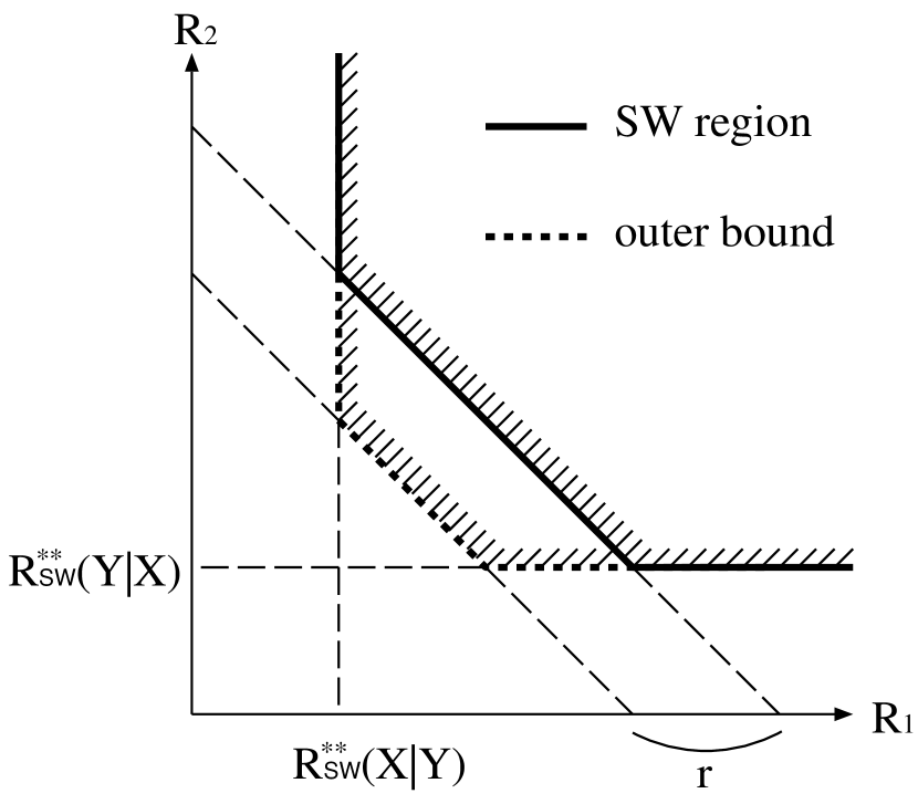
Figure 4: The outer bound given in Theorem 8.

Moreover, as shown in the theorem below, there exist $r$-totally sensitive function and a smooth source for which the outer bound given in Theorem 8 is tight.

Theorem 9.

For any $\delta>0$ and $0\leq r\leq\bar{r}$, there exist $r$-totally sensitive function $\bm{f}$ and a smooth source $(\bm{X},\bm{Y})$ such that

$$\mathcal{R}^{\mathsf{**}}(\bm{X},\bm{Y}|\bm{f}) \supseteq\left\{(R_{1},R_{2}):R_{1}\geq\delta+(1-\rho)\log\left\lvert\mathcal{X}\right\rvert,R_{2}\geq\delta+(1-\rho)\log\left\lvert\mathcal{Y}\right\rvert\right\}$$ (40)

and

$$\mathcal{R}_{\mathsf{SW}}^{\mathsf{**}}(\bm{X},\bm{Y}) \subseteq\bigl{\{}(R_{1},R_{2}):R_{1}\geq(1-\rho)\log\left\lvert\mathcal{X}\right\rvert,R_{2}\geq(1-\rho)\log\left\lvert\mathcal{Y}\right\rvert,$$

$$\qquad\qquad R_{1}+R_{2}\geq r-\delta+(1-\rho)\log\left\lvert\mathcal{X}\right\rvert\left\lvert\mathcal{Y}\right\rvert\bigr{\}}$$ (41)

where $\rho\triangleq r/\bar{r}$ and $\mathsf{**}=\mathsf{fl}/\mathsf{vl}$.

By taking $\delta\to 0$ in Theorem 9, we can make the bound (39) arbitrarily tight. Hence, our outer bound cannot be improved anymore only from $r$-total sensitivity and smooth condition.

III-E Moderate Deviation

In this subsection, we assume that $(\bm{X},\bm{Y})$ is an i.i.d. source with the joint distribution $P_{X_{1}Y_{1}}=P_{XY}$, and we consider the full side-information case. The results in Section III-B states that $R^{\mathsf{**}}(\bm{X}|\bm{Y}|\bm{f})=R_{\mathsf{SW}}^{\mathsf{**}}(\bm{X}|\bm{Y})=H(X|Y)$ ($\mathsf{**}=\mathsf{fl}/\mathsf{vl}$). In the following, we conduct more refined analysis in the moderate deviation regime.

For real numbers $t\in(0,1/2)$ and $\gamma>0$, and a sequence of functions $\bm{f}=\{f_{n}\}_{n=1}^{\infty}$, let

$$e^{\mathsf{vl}}(t,\gamma|\bm{f}) \triangleq\liminf_{n\to\infty}-\frac{1}{n^{1-2t}}\log\min_{\Phi_{n}}\mathrm{P}_{\mathrm{e}}(\Phi_{n}|f_{n})$$ (42)

where the minimum is taken over all sequences of codes $\{\Phi_{n}\}_{n=1}^{\infty}=\{(\varphi_{n}^{(1)},\psi_{n})\}_{n=1}^{\infty}$ for computing $\bm{f}=\{f_{n}\}_{n=1}^{\infty}$ satisfying

$$\limsup_{n\to\infty}\frac{1}{n^{1-t}}\left(\mathbb{E}\left[\left\lvert\varphi_{n}^{(1)}(X^{n})\right\rvert\right]-nH(X|Y)\right)\leq\gamma.$$ (43)

Similarly, by taking the minimum over all fixed-length codes, $e^{\mathsf{fl}}(t,\gamma|\bm{f})$ is defined. Further, by considering the identity function $f_{n}^{\mathsf{id}}$ and SW codes, $e_{\mathsf{SW}}^{\mathsf{vl}}(t,\gamma)$ and $e_{\mathsf{SW}}^{\mathsf{fl}}(t,\gamma)$ are defined. The single-letter characterization of $e_{\mathsf{SW}}^{\mathsf{vl}}(t,\gamma)$ and $e_{\mathsf{SW}}^{\mathsf{fl}}(t,\gamma)$ are obtained by He et. al.[11]. The following theorem states that computing sensitive function is as difficult as reproducing $\mathbf{X}$ itself even for the moderate deviation regime.

Theorem 10.

Suppose that $P_{XY}$ satisfies positivity condition and $\bm{f}$ is sensitive. Then, we have

$$e^{\mathsf{fl}}(t,\gamma|\bm{f}) =e_{SW}^{\mathsf{fl}}(t,\gamma),$$ (44)

$$e^{\mathsf{vl}}(t,\gamma|\bm{f}) =e_{SW}^{\mathsf{vl}}(t,\gamma)$$ (45)

for every $t\in(0,1/2)$ and $\gamma>0$.

IV Proof of Theorems

IV-A Preliminaries for Proofs

First we introduce some notations used in this section. $\bm{1}$ denotes the indicator function, e.g., $\bm{1}[s\in\mathcal{S}]=1$ if $s\in\mathcal{S}$ and $0$ otherwise; $h(p)$ is binary entropy function; $[a]^{+}$ is $0$ if $a<1$ and $\lfloor a\rfloor$ if $a\geq 1$. For given $0<\beta<1/2$, let

$$v_{n}(\beta) \triangleq\sum_{i=1}^{\lceil n\beta\rceil-1}(|\mathcal{X}|-1)^{i}\binom{n}{i}$$ (46)

$$\leq n|\mathcal{X}|^{n\beta}2^{nh(\beta)},$$ (47)

$$u_{n}(\beta) \triangleq\sum_{i=1}^{\lceil n\beta\rceil-1}(|\mathcal{Y}|-1)^{i}\binom{n}{i}$$ (48)

$$\leq n|\mathcal{Y}|^{n\beta}2^{nh(\beta)}.$$ (49)

For a given code $\Phi_{n}=(\varphi_{n}^{(1)},\varphi_{n}^{(2)},\psi_{n})$, we abbreviate the length of codewords by

$$\ell_{n}^{(1)}(\bm{x}) \triangleq\left\lvert\varphi_{n}^{(1)}(\bm{x})\right\rvert,$$ (50)

$$\ell_{n}^{(2)}(\bm{x}) \triangleq\left\lvert\varphi_{n}^{(2)}(\bm{x})\right\rvert.$$ (51)

Without loss of generality, we assume that there are $L_{1}<\infty$ and $L_{2}<\infty$ such that

$$\ell_{n}^{(1)}(\bm{x}) \leq nL_{1},~{}~{}~{}\mbox{for all }\bm{x}\in\mathcal{X}^{n},$$ (52)

$$\ell_{n}^{(2)}(\bm{x}) \leq nL_{2},~{}~{}~{}\mbox{for all }\bm{y}\in\mathcal{Y}^{n}.$$ (53)

Let

$$\mathcal{D}_{n}\triangleq\left\{(\bm{x},\bm{y}):\psi_{n}(\varphi_{n}^{(1)}(\bm{x}),\varphi_{n}^{(2)}(\bm{y}))=f_{n}(\bm{x},\bm{y})\right\}$$ (54)

be the set of all correctly decodable sequences. When we analyze the performance of a variable length code via information spectrum approach, the following typical-like sets play an important role:

$$\mathcal{T}_{n,1} \triangleq\left\{(\bm{x},\bm{y}):\frac{1}{n}\log\frac{1}{P_{X^{n}|Y^{n}}(\bm{x}|\bm{y})}\leq\frac{\ell_{n}^{(1)}(\bm{x})}{n}+\delta\right\},$$ (55)

$$\mathcal{T}_{n,2} \triangleq\left\{(\bm{x},\bm{y}):\frac{1}{n}\log\frac{1}{P_{Y^{n}|X^{n}}(\bm{y}|\bm{x})}\leq\frac{\ell_{n}^{(2)}(\bm{y})}{n}+\delta\right\},$$ (56)

$$\mathcal{T}_{n,0} \triangleq\left\{(\bm{x},\bm{y}):\frac{1}{n}\log\frac{1}{P_{X^{n}Y^{n}}(\bm{x},\bm{y})}\leq\frac{\ell_{n}^{(1)}(\bm{x})}{n}+\frac{\ell_{n}^{(2)}(\bm{y})}{n}+\delta\right\},$$ (57)

where $\delta>0$ is any real number specified later. The following lemma is the core of the proofs of coding theorems, which connect the combinatorial property, i.e., the sensitivity of a function, to a probabilistic analysis. The proof of the lemma will be given in Appendix C.

Lemma 1.

For any code $\Phi_{n}$ and real numbers $\beta,\delta>0$, if $f_{n}$ is sensitive conditioned on $\mathcal{Y}^{n}$ and $(\bm{X},\bm{Y})$ is smooth with respect to $\bm{Y}$, then we have

$$P_{X^{n}Y^{n}}(\mathcal{D}_{n}\cap\mathcal{T}_{n,1}^{c}) \leq\frac{2|\mathcal{Y}|}{\beta q}\mathrm{P}_{\mathrm{e}}(\Phi_{n}|f_{n})+(v_{n}(\beta)+1)2^{-n\delta}.$$ (58)

Similarly, if $f_{n}$ is sensitive conditioned on $\mathcal{X}^{n}$ and $(\bm{X},\bm{Y})$ is smooth with respect to $\bm{X}$, then we have

$$P_{X^{n}Y^{n}}(\mathcal{D}_{n}\cap\mathcal{T}_{n,2}^{c}) \leq\frac{2|\mathcal{X}|}{\beta q}\mathrm{P}_{\mathrm{e}}(\Phi_{n}|f_{n})+(u_{n}(\beta)+1)2^{-n\delta}.$$ (59)

Furthermore, if $f_{n}$ is totally sensitive and $(\bm{X},\bm{Y})$ is smooth, then we have

$$P_{X^{n}Y^{n}}(\mathcal{D}_{n}\cap\mathcal{T}_{n,0}^{c}) \leq\frac{2(|\mathcal{X}|+|\mathcal{Y}|)}{\beta q}\mathrm{P}_{\mathrm{e}}(\Phi_{n}|f_{n})+[(v_{n}(\beta)+1)+(u_{n}(\beta)+1)]2^{-n\delta}.$$ (60)

The following lemma is an immediate consequence of Lemma 1.

Lemma 2.

For any $\delta>0$ and any code satisfying (5), if $\bm{f}$ is totally sensitive, we have

$$\lim_{n\to\infty}P_{X^{n}Y^{n}}(\mathcal{T}_{n,1}^{c}\cup\mathcal{T}_{n,2}^{c}\cup\mathcal{T}_{n,0}^{c})=0.$$ (61)

Proof:

We have

$$P_{X^{n}Y^{n}}(\mathcal{T}_{n,1}^{c}\cup\mathcal{T}_{n,2}^{c}\cup\mathcal{T}_{n,0}^{c})$$

$$=P_{X^{n}Y^{n}}(\mathcal{D}_{n}^{c}\cap(\mathcal{T}_{n,1}^{c}\cup\mathcal{T}_{n,2}^{c}\cup\mathcal{T}_{n,0}^{c}))+P_{X^{n}Y^{n}}(\mathcal{D}_{n}\cap(\mathcal{T}_{n,1}^{c}\cup\mathcal{T}_{n,2}^{c}\cup\mathcal{T}_{n,0}^{c}))$$ (62)

$$\leq\mathrm{P}_{\mathrm{e}}(\Phi_{n}|f_{n})+P_{X^{n}Y^{n}}(\mathcal{D}_{n}\cap\mathcal{T}_{n,1}^{c})+P_{X^{n}Y^{n}}(\mathcal{D}_{n}\cap\mathcal{T}_{n,2}^{c})+P_{X^{n}Y^{n}}(\mathcal{D}_{n}\cap\mathcal{T}_{n,0}^{c}).$$ (63)

Then, we apply Lemma 1 by taking sufficiently small $\beta>0$ so that $v_{n}(\beta)2^{-n\delta}$ and $u_{n}(\beta)2^{-n\delta}$ converges to $0$ as $n\to\infty$. ∎

IV-B Proof of Theorem 1

For a given (variable-length) code $\Phi_{n}$ for function computation, we construct a SW code by using a random binning of adaptive length. Let

$$\tilde{\ell}_{n}^{(1)}(\bm{x}) \triangleq\lceil\ell_{n}^{(1)}(\bm{x})+2n\delta\rceil,$$ (64)

$$\tilde{\ell}_{n}^{(2)}(\bm{x}) \triangleq\lceil\ell_{n}^{(2)}(\bm{x})+2n\delta\rceil,$$ (65)

and for each integer $l$, let

$$\mathcal{S}_{n,1}(l) \triangleq\left\{(\bm{x},\bm{y}):\frac{1}{n}\log\frac{1}{P_{X^{n}|Y^{n}}(\bm{x}|\bm{y})}\leq\frac{l}{n}-\delta\right\},$$ (66)

$$\mathcal{S}_{n,2}(l) \triangleq\left\{(\bm{x},\bm{y}):\frac{1}{n}\log\frac{1}{P_{Y^{n}|X^{n}}(\bm{y}|\bm{x})}\leq\frac{l}{n}-\delta\right\},$$ (67)

$$\mathcal{S}_{n,0}(l) \triangleq\left\{(\bm{x},\bm{y}):\frac{1}{n}\log\frac{1}{P_{X^{n}Y^{n}}(\bm{x},\bm{y})}\leq\frac{l}{n}-\delta\right\}.$$ (68)

Further, for integers $l_{1}$ and $l_{2}$, let

$$\mathcal{S}_{n}(l_{1},l_{2})\triangleq\mathcal{S}_{n,1}(l_{1})\cap\mathcal{S}_{n,2}(l_{2})\cap\mathcal{S}_{n,0}(l_{1}+l_{2}).$$ (69)

Note that, for any $\bm{y}\in\mathcal{Y}^{n}$, we have

$$|\{\hat{\bm{x}}:(\hat{\bm{x}},\bm{y})\in\mathcal{S}_{n}(l_{1},l_{2})\}| \leq|\{\hat{\bm{x}}:(\hat{\bm{x}},\bm{y})\in\mathcal{S}_{n,1}(l_{1})\}|$$ (70)

$$\leq 2^{l_{1}-n\delta}.$$ (71)

Similarly, for any $\bm{x}\in\mathcal{X}^{n}$, we have

$$|\{\hat{\bm{y}}:(\bm{x},\hat{\bm{y}})\in\mathcal{S}_{n}(l_{1},l_{2})\}|\leq 2^{l_{2}-n\delta}$$ (72)

and

$$|\{(\hat{\bm{x}},\hat{\bm{y}}):(\hat{\bm{x}},\hat{\bm{y}})\in\mathcal{S}_{n}(l_{1},l_{2})\}|\leq 2^{l_{1}+l_{2}-n\delta}.$$ (73)

Now, we construct a SW code as follows:

• Given $\bm{x}\in\mathcal{X}^{n}$, the encoder 1

  1. sends the integer $l_{1}=\tilde{\ell}_{n}^{(1)}(\bm{x})$ by using at most $2(\lfloor\log\tilde{\ell}_{n}^{(1)}(\bm{x})\rfloor+1)$ bits [18], and then

  2. by using a random bin-code with $\tilde{\ell}_{n}^{(1)}(\bm{x})$ bits, sends the bin-index $m_{1}$ of $\bm{x}$.

• Given $\bm{y}\in\mathcal{Y}^{n}$, the encoder 2

  1. sends the integer $l_{2}=\tilde{\ell}_{n}^{(2)}(\bm{y})$ by using at most $2(\lfloor\log\tilde{\ell}_{n}^{(1)}(\bm{x})\rfloor+1)$ bits [18], and then

  2. by using a random bin-code with $\tilde{\ell}_{n}^{(2)}(\bm{y})$ bits, sends the bin-index $m_{2}$ of $\bm{y}$.

• The decoder

  1. extracts $l_{1}$, $l_{2}$, $m_{1}$, and $m_{2}$ from the received codewords, and then

  2. looks for the unique pair $(\bm{x},\bm{y})$ such that $(\bm{x},\bm{y})\in\mathcal{S}_{n}(l_{1},l_{2})$, $\tilde{\ell}_{n}^{(1)}(\bm{x})=l_{1}$, $\tilde{\ell}_{n}^{(2)}(\bm{y})=l_{2}$, and the bin-index of $\bm{x}$ (resp. $\bm{y}$) is $m_{1}$ (resp. $m_{2}$).

By using the standard argument, we can upper bound the average error probability $\mathbb{E}[\mathrm{P}_{\mathrm{e}}(\hat{\Phi}_{n}|f_{n}^{\mathsf{id}})]$ of the constructed SW code with respect to random bin-coding by

$$\mathbb{E}[\mathrm{P}_{\mathrm{e}}(\hat{\Phi}_{n}|f_{n}^{\mathsf{id}})] \leq\Pr\Bigg{\{}\frac{1}{n}\log\frac{1}{P_{X^{n}|Y^{n}}(X^{n}|Y^{n})}>\frac{\tilde{\ell}_{n}^{(1)}(X^{n})}{n}-\delta\text{ or }$$

$$~{}~{}~{}\frac{1}{n}\log\frac{1}{P_{Y^{n}|X^{n}}(Y^{n}|X^{n})}>\frac{\tilde{\ell}_{n}^{(2)}(Y^{n})}{n}-\delta\text{ or }$$

$$~{}~{}~{}\frac{1}{n}\log\frac{1}{P_{X^{n}Y^{n}}(X^{n},Y^{n})}>\frac{\tilde{\ell}_{n}^{(1)}(X^{n})+\tilde{\ell}_{n}^{(2)}(Y^{n})}{n}-\delta\Bigg{\}}$$

$$+\sum_{\bm{x},\bm{y}}P_{X^{n}Y^{n}}(\bm{x},\bm{y})\frac{\left|\left\{\hat{\bm{x}}:(\hat{\bm{x}},\bm{y})\in\mathcal{S}_{n}(\tilde{\ell}_{n}^{(1)}(\bm{x}),\tilde{\ell}_{n}^{(2)}(\bm{y}))\right\}\right|}{2^{\tilde{\ell}_{n}^{(1)}(\bm{x})}}$$

$$+\sum_{\bm{x},\bm{y}}P_{X^{n}Y^{n}}(\bm{x},\bm{y})\frac{\left|\left\{\hat{\bm{y}}:(\bm{x},\hat{\bm{y}})\in\mathcal{S}_{n}(\tilde{\ell}_{n}^{(1)}(\bm{x}),\tilde{\ell}_{n}^{(2)}(\bm{y}))\right\}\right|}{2^{\tilde{\ell}_{n}^{(2)}(\bm{y})}}$$

$$+\sum_{\bm{x},\bm{y}}P_{X^{n}Y^{n}}(\bm{x},\bm{y})\frac{\left|\left\{\hat{\bm{x}}:(\hat{\bm{x}},\hat{\bm{y}})\in\mathcal{S}_{n}(\tilde{\ell}_{n}^{(1)}(\bm{x}),\tilde{\ell}_{n}^{(2)}(\bm{y}))\right\}\right|}{2^{\tilde{\ell}_{n}^{(1)}(\bm{x})+\tilde{\ell}_{n}^{(2)}(\bm{y})}}$$ (74)

$$\leq\Pr\Bigg{\{}\frac{1}{n}\log\frac{1}{P_{X^{n}|Y^{n}}(X^{n}|Y^{n})}>\frac{\ell_{n}^{(1)}(X^{n})}{n}+\delta\text{ or }$$

$$~{}~{}~{}\frac{1}{n}\log\frac{1}{P_{Y^{n}|X^{n}}(Y^{n}|X^{n})}>\frac{\ell_{n}^{(2)}(Y^{n})}{n}+\delta\text{ or }$$

$$~{}~{}~{}\frac{1}{n}\log\frac{1}{P_{X^{n}Y^{n}}(X^{n},Y^{n})}>\frac{\ell_{n}^{(1)}(X^{n})+\ell_{n}^{(2)}(Y^{n})}{n}+\delta\Bigg{\}}+3\cdot 2^{-n\delta}$$ (75)

$$=P_{X^{n}Y^{n}}(\mathcal{T}_{n,1}^{c}\cup\mathcal{T}_{n,2}^{c}\cup\mathcal{T}_{n,0}^{c})+3\cdot 2^{-n\delta}.$$ (76)

Hence, by Lemma 2, we have $\mathbb{E}[\mathrm{P}_{\mathrm{e}}(\hat{\Phi}_{n}|f_{n}^{\mathsf{id}})]\to 0$ as $n\to\infty$. This implies that there exists a SW code $\hat{\Phi}_{n}=(\hat{\varphi}_{n}^{(1)},\hat{\varphi}_{n}^{(2)},\hat{\psi}_{n})$ satisfying (27).

On the other hand, the codeword length of the encoder $\hat{\varphi}_{n}^{(1)}$ of the constructed SW code satisfies that

$$\left\lvert\hat{\varphi}_{n}^{(1)}(\bm{x})\right\rvert \leq\tilde{\ell}_{n}^{(1)}(\bm{x})+2(\lfloor\log\tilde{\ell}_{n}^{(1)}(\bm{x})\rfloor+1)$$ (77)

$$\leq\ell_{n}^{(1)}(\bm{x})+2n\delta+2\log(\ell_{n}^{(1)}(\bm{x})+2n\delta)+3$$ (78)

$$\leq\ell_{n}^{(1)}(\bm{x})+2n\delta+2\log(nL_{1}+2n\delta)+3.$$ (79)

Since we can take $\delta>0$ arbitrarily small, $\hat{\varphi}_{n}^{(1)}$ satisfies (28). Similarly, we can prove (29). ∎

IV-C Proof of Theorem 3 and Theorem 4

Since “if” part is obvious from Theorem 2, we only prove “only if” part. When a function is symbol-wise but not sensitive conditioned on $\mathcal{X}$ or $\mathcal{Y}$, then it does not satisfy Condition 1 or Condition 2 in Definition 8. Thus, the result in [5] implies that the Slepian-Wolf region can be improved. Hence, it suffice to consider a symbol-wise function that is sensitive condition on $\mathcal{X}$ and $\mathcal{Y}$, but not jointly sensitive.

Let us consider a class of finite-state sources such that

$$P_{X^{2n}Y^{2n}}(\bm{x},\bm{y})=\prod_{i=1}^{n}P_{X^{2}Y^{2}}(x_{2i-1}x_{2i},y_{2i-1}y_{2i}).$$ (80)

In other words, let us consider a class of two-symbol-wise i.i.d. sources. Note that such a source $(\bm{X},\bm{Y})$ includes an i.i.d. source $(\bm{U},\bm{V})$ with alphabets $\mathcal{U}=\mathcal{X}^{2}$ and $\mathcal{V}=\mathcal{Y}^{2}$.

Assume that $\bm{f}$ is symbol-wise but not jointly sensitive. Then, as shown in the proof of Proposition 1, there exists $x^{2}=(a_{0},a_{1})$, $\hat{x}^{2}=(a_{0},a_{2})$, $y^{2}=(b_{1},b_{0})$, and $\hat{y}^{2}=(b_{2},b_{0})$ such that $x^{2}\neq\hat{x}^{2}$, $y^{2}\neq\hat{y}^{2}$, and $f_{2}(x^{2},y^{2})=f_{2}(\hat{x}^{2},\hat{y}^{2})$. Note that $f$ induces a function $g$ on $\mathcal{U}\times\mathcal{V}$ which is not an HK function.

Now, we can prove the theorem by applying the result of Han and Kobayashi [5, Theorem 1] to $(\bm{U},\bm{V})$ and $g_{n}(\bm{u},\bm{v})=(g(u_{1},v_{1}),\ldots,g(u_{n},v_{n}))$; it should be noted that, while Han and Kobayashi deal with fixed length coding, the SW region for fixed length coding is identical with that of variable length coding if the source is i.i.d.. Further, it is not hard to see that $(\bm{X},\bm{Y})$ is smooth if $(\bm{U},\bm{V})$ satisfies the positivity condition, i.e., $P_{UV}(u,v)>0$ for all $(u,v)$. ∎

IV-D Proofs of Theorem 5 and Theorem 6

The proof of these theorems are almost the same as that of Theorem 1. Thus, we only show the outline. For a given variable-length code $\Phi_{n}=(\varphi_{n}^{(1)},\psi_{n})$ for computing $f_{n}$, by a similar argument as Section IV-B, we can show that there exists a SW code (with full side-information) $\hat{\Phi}_{n}=(\hat{\varphi}_{n}^{(1)},\hat{\psi}_{n})$ satisfying

$$\mathrm{P}_{\mathrm{e}}(\hat{\Phi}_{n}|f_{n}^{\mathsf{id}}) \leq P_{X^{n}Y^{n}}(\mathcal{T}_{n,1}^{c})+2^{-n\delta}$$ (81)

$$=P_{X^{n}Y^{n}}(\mathcal{D}_{n}^{c}\cap\mathcal{T}_{n,1}^{c})+P_{X^{n}Y^{n}}(\mathcal{D}_{n}\cap\mathcal{T}_{n,1}^{c})+2^{-n\delta}$$ (82)

$$\leq\mathrm{P}_{\mathrm{e}}(\Phi_{n}|f_{n})+P_{X^{n}Y^{n}}(\mathcal{D}_{n}\cap\mathcal{T}_{n,1}^{c})+2^{-n\delta}$$ (83)

and

$$\left\lvert\hat{\varphi}_{n}^{(1)}(\bm{x})\right\rvert\leq\ell_{n}^{(1)}(\bm{x})+2n\delta+2\log(nL_{1}+2n\delta)+3.$$ (84)

Now, we apply Lemma 1 to (83), and obtain

$$\mathrm{P}_{\mathrm{e}}(\hat{\Phi}_{n}|f_{n}^{\mathsf{id}})\leq\left(1+\frac{2|\mathcal{Y}|}{\beta q}\right)\mathrm{P}_{\mathrm{e}}(\Phi_{n}|f_{n})+(v_{n}(\beta)+2)2^{-n\delta}.$$ (85)

Thus, by taking $\beta>0$ sufficiently small compared to $\delta>0$, we can derive the statement of the theorem. ∎

IV-E Proof of Theorem 7

The only modifications we need is the proof of Lemma 1. In the proof of Lemma 1, we use the properties of sensitivity and smooth in (119) and (120). Suppose that $P_{X^{n}Y^{n}}(\bm{x}_{k}^{\prime},\bm{y})\cdot P_{X^{n}Y^{n}}(\bm{x}_{k}^{\prime\prime},\bm{y})>0$ (otherwise, since $P_{X^{n}Y^{n}}(\bm{x}_{v+2k},\bm{y})=0$, the desired inequality $P_{X^{n}Y^{n}}(\bm{x}_{k,j}^{*},\bm{y}_{j})\geq qP_{X^{n}Y^{n}}(\bm{x}_{v+2k},\bm{y})$ holds trivially) and $\bm{x}_{k}^{\prime}$ and $\bm{x}_{k}^{\prime\prime}$ differ in $i_{1}$th, …, $i_{\lceil\beta n\rceil}$th positions. Since $(\bm{X},\bm{Y})$ is weakly smooth, for each $j=1,\ldots,\lceil\beta n\rceil$, there exists $\bm{y}_{j}$ that differs from $\bm{y}$ only in $i_{j}$th position and

$$P_{X^{n}Y^{n}}(\bm{x}_{k}^{\prime},\bm{y}_{j}) \geq qP_{X^{n}Y^{n}}(\bm{x}_{k}^{\prime},\bm{y}),$$ (86)

$$P_{X^{n}Y^{n}}(\bm{x}_{k}^{\prime\prime},\bm{y}_{j}) \geq qP_{X^{n}Y^{n}}(\bm{x}_{k}^{\prime\prime},\bm{y}).$$ (87)

Furthermore, since $f_{n}$ is highly sensitive conditioned on $\mathcal{Y}^{n}$, we have $f_{n}(\bm{x}_{k}^{\prime},\bm{y}_{j})\neq f_{n}(\bm{x}_{k}^{\prime\prime},\bm{y}_{j})$, which implies either of the events in (119) is true. Then, by defining $\bm{x}_{k,j}^{*}$ in the same manner as the proof of Lemma 1, (120) also holds. The rest of the proof goes through exactly in the same manner. ∎

IV-F Proof of Theorem 8

The key of the proof is to modify (60) in Lemma 1 as follows: Under the assumption of the theorem, we have

$$P_{X^{n}Y^{n}}(\mathcal{D}_{n}\cap\tilde{\mathcal{T}}_{n,0}^{c}) \leq\frac{2(|\mathcal{X}|+|\mathcal{Y}|)}{\beta q}\mathrm{P}_{\mathrm{e}}(\Phi_{n}|f_{n})+[(v_{n}(\beta)+1)+(u_{n}(\beta)+1)]2^{-n\delta}$$ (88)

where

$$\tilde{\mathcal{T}}_{n,0} \triangleq\left\{(\bm{x},\bm{y}):\frac{1}{n}\log\frac{1}{P_{X^{n}Y^{n}}(\bm{x},\bm{y})}\leq\frac{\ell_{n}^{(1)}(\bm{x})}{n}+\frac{\ell_{n}^{(2)}(\bm{y})}{n}+r+2\delta\right\}.$$ (89)

Then, by using the same construction as the proof of Theorem 1, we can show that, for any $\lambda\in[0,1]$, there exists a SW code $\hat{\Phi}_{n}=(\hat{\varphi}_{n}^{(1)},\hat{\varphi}_{n}^{(2)},\hat{\psi}_{n})$ satisfying (27) and

$$\left\lvert\hat{\varphi}_{n}^{(1)}(\bm{x})\right\rvert \leq\ell_{n}^{(1)}(\bm{x})+2n\delta+2\log(nL_{1}+2n\delta)+2+n\lambda r,$$ (90)

$$\left\lvert\hat{\varphi}_{n}^{(2)}(\bm{y})\right\rvert \leq\ell_{n}^{(2)}(\bm{y})+2n\delta+2\log(nL_{1}+2n\delta)+2+n(1-\lambda)r.$$ (91)

Hence, we have

$$\mathcal{R}^{\mathsf{**}}(\bm{X},\bm{Y}|\bm{f}) \subseteq\left\{(R_{1},R_{2}):0\leq\exists\lambda\leq 1,(R_{1}+\lambda r,R_{2}+(1-\lambda)r)\in\mathcal{R}_{\mathsf{SW}}^{\mathsf{**}}(\bm{X},\bm{Y})\right\}.$$ (92)

On the other hand, note that $f_{n}$ is sensitive conditioned on both of $\mathcal{X}^{n}$ and $\mathcal{Y}^{n}$ by the definition of $r$-total sensitivity. Hence, from Theorems 5 and 6, we have

$$\mathcal{R}^{\mathsf{**}}(\bm{X},\bm{Y}|\bm{f}) \subseteq\left\{(R_{1},R_{2}):R_{1}\geq R_{\mathsf{SW}}^{\mathsf{**}}(\bm{X}|\bm{Y}),R_{2}\geq R_{\mathsf{SW}}^{\mathsf{**}}(\bm{Y}|\bm{X})\right\}.$$ (93)

Combining (92) and (93), we have the theorem.

Now, we prove (88). Since (88) is a modification of (60), we explain how the proof of (60), which is given in Appendix C, is modified to prove (88).

Since (38) holds, for sufficiently large $n$ and for any $z_{n}\in\mathcal{Z}_{n}$, we have

$$\mathsf{Equiv}(z_{n}|f_{n})\leq 2^{n(r+\delta)}.$$ (94)

This guarantees that, instead of (130), we can find $(\bm{x}_{1},\bm{y}_{1}),\dots,(\bm{x}_{J},\bm{y}_{J})$ such that $\bm{x}_{i}\neq\bm{x}_{j}$ and $\bm{y}_{i}\neq\bm{y}_{j}$ for every $i\neq j$, $J\leq 2^{n(r+\delta)}$, and

$$\mathcal{D}_{a,b}\subseteq\bigcup_{i=1}^{J}\left[(\mathcal{D}_{a,\bm{y}_{i}}\times\{\bm{y}_{i}\})\cup(\{\bm{x}_{i}\}\times\mathcal{D}_{\bm{x}_{i},b})\right].$$ (95)

Thus, instead of (133), we have

$$P_{X^{n}Y^{n}}(\mathcal{D}\cap\tilde{\mathcal{T}}_{0}^{c})$$

$$\leq\sum_{a\in\mathcal{C}^{(1)}}\sum_{b\in\mathcal{C}^{(2)}}\left[\sum_{i=1}^{J}\sum_{\bm{x}\in\mathcal{D}_{a,\bm{y}_{i}}}P_{X^{n}Y^{n}}(\bm{x},\bm{y}_{i})\bm{1}[(\bm{x},\bm{y}_{i})\in\tilde{\mathcal{T}}_{0}^{c}]+\sum_{i=1}^{J}\sum_{\bm{y}\in\mathcal{D}_{\bm{x}_{i},b}}P_{X^{n}Y^{n}}(\bm{x}_{i},\bm{y})\bm{1}[(\bm{x}_{i},\bm{y})\in\tilde{\mathcal{T}}_{0}^{c}]\right]$$ (96)

$$\leq\sum_{a\in\mathcal{C}^{(1)}}\sum_{b\in\mathcal{C}^{(2)}}J[(v+1)+(u+1)]2^{-\ell(a)-\ell(b)-r-2n\delta}$$

$$+\sum_{a\in\mathcal{C}^{(1)}}\sum_{b\in\mathcal{C}^{(2)}}\sum_{i=1}^{J}\sum_{k=1}^{\left[\frac{1}{2}(|\mathcal{D}_{a,\bm{y}_{i}}|-v)\right]^{+}}\left(P_{X^{n}Y^{n}}(\bm{x}_{v+2k},\bm{y}_{i})+P_{X^{n}Y^{n}}(\bm{x}_{v+2k+1},\bm{y}_{i})\right)$$

$$+\sum_{a\in\mathcal{C}^{(1)}}\sum_{b\in\mathcal{C}^{(2)}}\sum_{i=1}^{J}\sum_{k=1}^{\left[\frac{1}{2}(|\mathcal{D}_{\bm{x}_{i},b}|-u)\right]^{+}}\left(P_{X^{n}Y^{n}}(\bm{x}_{i},\bm{y}_{u+2k})+P_{X^{n}Y^{n}}(\bm{x}_{i},\bm{y}_{u+2k+1})\right).$$ (97)

Then, each term in (97) is upper bounded in the same way as (134), (136), and (137) respectively. Hence, we have (88). ∎

IV-G Proof of Theorem 9

Let $\mathsf{p}$ be the smallest prime integer larger than $\left\lvert\mathcal{X}\right\rvert+\left\lvert\mathcal{Y}\right\rvert-2$ and consider a Galois field $\mathsf{GF}(\mathsf{p})=\{0,1,\dots,\mathsf{p}-1\}$. Without loss of generality, we assume that $\mathcal{X}=\{0,1,\dots,\left\lvert\mathcal{X}\right\rvert-1\}\subseteq\mathsf{GF}(\mathsf{p})$ and $\mathcal{Y}=\{0,1,\dots,\left\lvert\mathcal{Y}\right\rvert-1\}\subseteq\mathsf{GF}(\mathsf{p})$. Then, let us define the function $f_{n}$ as

$$f_{n}(\bm{x},\bm{y}) \triangleq\left(x_{1}\oplus y_{1},x_{2}\oplus y_{2},\dots x_{n\rho}\oplus y_{n\rho},(x_{n\rho+1},y_{n\rho+1}),(x_{n\rho+2},y_{n\rho+2}),\dots,(x_{n},y_{n})\right)$$ (98)

where $\oplus$ is addition in $\mathsf{GF}(\mathsf{p})$. In other words, the first $n\rho$ symbols of $f_{n}(\bm{x},\bm{y})$ is symbol-wise addition in $\mathsf{GF}(\mathsf{p})$ and the remaining part of $f_{n}(\bm{x},\bm{y})$ is identical with the last $n(1-\rho)$ symbols of $(\bm{x},\bm{y})$. We can see that $\bm{f}=\{f_{n}\}_{n=1}^{\infty}$ is $r$-totally sensitive, since $\max_{z_{n}\in\mathcal{Z}_{n}}\mathsf{Equiv}(z_{n}|f_{n})=M^{n\rho}=2^{nr}$, where $M\triangleq\min\{\left\lvert\mathcal{X}\right\rvert,\left\lvert\mathcal{Y}\right\rvert\}=2^{\bar{r}}$.

On the other hand, we consider a general source $(\bm{X},\bm{Y})$ defined as follows. Fix $\varepsilon>0$ specified later, and let $Q_{XY}$ be a joint distribution on $\mathcal{X}\times\mathcal{Y}$ such that

$$Q_{XY}(x,y) =\begin{cases}\frac{1-\varepsilon}{M}&(x,y)=(0,M-1),(1,M-2),\dots,(M-1,0),\\ \frac{\varepsilon}{\left\lvert\mathcal{X}\right\rvert\left\lvert\mathcal{Y}\right\rvert-M}&\text{otherwise}.\end{cases}$$ (99)

Then, let us define the joint distribution of $(X^{n},Y^{n})$ as

$$P_{X^{n}Y^{n}}(\bm{x},\bm{y}) =\left[\prod_{i=1}^{n\rho}Q_{XY}(x_{i},y_{i})\right]\times\left(\frac{1}{\left\lvert\mathcal{X}\right\rvert\left\lvert\mathcal{Y}\right\rvert}\right)^{n(1-\rho)}$$ (100)

for all $(\bm{x},\bm{y})$. That is, the first $n\rho$ symbols of $(X^{n},Y^{n})$ is i.i.d. with the joint distribution $Q_{XY}$ and the last $n(1-\rho)$ symbols of $(X^{n},Y^{n})$ is i.i.d. with the uniform distribution on $\mathcal{X}\times\mathcal{Y}$. We can see that $(\bm{X},\bm{Y})\triangleq\{(X^{n},Y^{n})\}_{n=1}^{\infty}$ is smooth, since $Q_{XY}$ satisfies the positivity condition.

Now, we prove that (40) and (41) hold for $\bm{f}$ and $(\bm{X},\bm{Y})$ defined above.

At first, let us construct a coding scheme for computing $f_{n}$ as follows: (i) The first $n\rho$ symbols are coded by the coding scheme given in Lemma 5 of [5]; i.e., a generalization of the coding scheme of Körner and Marton [1]. (ii) The remaining $n(1-\rho)$ symbols are sent to the decoder without compression. Note that if $(X,Y)\sim Q_{XY}$ and $\varepsilon$ is sufficiently small then

$$H(X\oplus Y)\leq h(\varepsilon)+\varepsilon\log\left(\left\lvert\mathcal{X}\right\rvert\left\lvert\mathcal{Y}\right\rvert-M\right)\leq\delta/\rho.$$ (101)

Thus, by the coding scheme described above, the pair $(R_{1},R_{2})$ satisfying $R_{1}\geq\delta+(1-\rho)\log\left\lvert\mathcal{X}\right\rvert$ and $R_{2}\geq\delta+(1-\rho)\log\left\lvert\mathcal{Y}\right\rvert$ is achievable. Hence, we have (40).

On the other hand, note that if $(X,Y)\sim Q_{XY}$ and $\varepsilon$ is sufficiently small then

$$H(X,Y) =(1-\varepsilon)\log M+h(\varepsilon)+\varepsilon\log\left(\left\lvert\mathcal{X}\right\rvert\left\lvert\mathcal{Y}\right\rvert-M\right)$$ (102)

$$\geq\bar{r}-\delta/\rho.$$ (103)

Hence, from (100), we have

$$H(X^{n}|Y^{n}) \geq n(1-\rho)\log\left\lvert\mathcal{X}\right\rvert$$ (104)

$$H(Y^{n}|X^{n}) \geq n(1-\rho)\log\left\lvert\mathcal{X}\right\rvert$$ (105)

and

$$H(X^{n},Y^{n}) \geq n\rho(\bar{r}-\delta/\rho)+n(1-\rho)\log\left\lvert\mathcal{X}\right\rvert\left\lvert\mathcal{Y}\right\rvert$$ (106)

$$=n\left\{r-\delta+(1-\rho)\log\left\lvert\mathcal{X}\right\rvert\left\lvert\mathcal{Y}\right\rvert\right\}.$$ (107)

From (104)–(107), it is not hard to see that (41) holds. ∎

IV-H Proof of Theorem 10

We only prove (45) since (44) can be proved in a similar manner. It suffice to prove only one direction, i.e., $e^{\mathsf{vl}}(t,\gamma|\bm{f})\leq e_{SW}^{\mathsf{vl}}(t,\gamma)$. For a given code $\{\Phi_{n}\}_{n=1}^{\infty}$ satisfying (43) and

$$\liminf_{n\to\infty}-\frac{1}{n^{1-2t}}\log\mathrm{P}_{\mathrm{e}}(\Phi_{n}|f_{n})\geq e^{\mathsf{vl}}(t,\gamma|\bm{f}),$$ (108)

we can construct a SW code $\hat{\Phi}_{n}=(\hat{\varphi}_{n}^{(1)},\hat{\psi}_{n})$ satisfying (84) and (85). We set $\beta=\beta_{n}=\frac{1}{n}$ and $\delta=\delta_{n}=\frac{1}{n^{3t/2}}$. Then, by noting $h(\beta)\leq 2\beta+2\beta\log(1/2\beta)$ for $0<\beta<1/2$, we have $v_{n}(\beta_{n})\leq 16|\mathcal{X}|n^{3}$. Thus, we have

$$\limsup_{n\to\infty}\frac{1}{n^{1-t}}\left(\mathbb{E}\left[\left\lvert\hat{\varphi}_{n}^{(1)}(X^{n})\right\rvert\right]-nH(X|Y)\right)\leq\gamma$$ (109)

and

$$\liminf_{n\to\infty}-\frac{1}{n^{1-2t}}\log\mathrm{P}_{\mathrm{e}}(\hat{\Phi}_{n}|f_{n}^{\mathsf{id}})\geq e^{\mathsf{vl}}(t,\gamma|\bm{f}).$$ (110)

V Conclusion

In this paper, we investigated a dichotomy of functions in distributed coding: for a sequence $\bm{f}$ of functions, does the achievable rate region for computing $\bm{f}$ coincide with the SW region? We introduced the class of smooth sources and gave a sufficient condition for the coincidence: if $\bm{f}$ is totally sensitive then the achievable rate region for computing $\bm{f}$ coincides with the SW region for any smooth sources. Further, we proved that, for symbol-wise functions, the total sensitivity is the necessary and sufficient condition for the coincidence of two regions. On the other hand, it remains as a future work to establish the necessary and sufficient condition on functions which may not be symbol-wise.

Moreover, as a generalization of our dichotomy theorem, we give an outer bound on the achievable rate region for computing a class of functions wider than the totally sensitive functions. Of course, to characterize the achievable rate region for general functions remains as a future work.

In our investigation, we used the information-spectrum approach so that we can establish the results in a unified way. This approach allows us to derive a refined result in the moderate deviation regime as given in Section III-E. Although we consider only i.i.d. sources in Section III-E for simplicity, it is not hard to generalize Theorem 10 for wider classes of sources. Indeed, the assumption of i.i.d. is not so critical in the proof of Theorem 10 given in Section IV-H. On the other hand, for general sources that have memory and may not be stationary nor ergodic, to characterize $e_{\mathsf{SW}}^{\mathsf{vl}}(t,\gamma)$ and $e_{\mathsf{SW}}^{\mathsf{fl}}(t,\gamma)$ itself remains as an important work.

In this paper, we considered only lossless computation, where the error probability is required to tend zero as the block size goes to infinity. It is an important future work to generalize our results for $\varepsilon$-error case, where the error probability is required only to be smaller than the given threshold $\varepsilon>0$. When we consider $\varepsilon$-error case, the strong converse property is an important subject to be investigated; e.g., it is an interesting problem to establish the necessary and sufficient condition on functions so that the strong converse holds for function computation whenever the strong converse holds for SW coding. Furthermore, it is also an important future work to generalize our results for lossy case and to establish the condition so that the rate-distortion region for distributed computing coincides with that for distributed source coding.

Appendix A Proof of Proposition 1

If part

At first, we assume that $f$ is an HK function and satisfies 1) of the proposition. Then we have

$$f(a_{1},b_{1})=f(a_{2},b_{2})\text{ means }b_{1}=b_{2}.$$ (111)

Indeed, if $a_{1}=a_{2}$ then (111) follows from 1) of the proposition. Moreover, if $a_{1}\neq a_{2}$ then (111) follows from the condition 3) in the definition of HK functions.

Now, note that if $f_{n}(\bm{x},\bm{y})=f_{n}(\hat{\bm{x}},\hat{\bm{y}})$ then $f(x_{i},y_{i})=f(\hat{x}_{i},\hat{y}_{i})$ for all $i=1,2,\dots,n$, since $f_{n}$ is symbol-wise. Hence, by (111), we can see that if $f_{n}(\bm{x},\bm{y})=f_{n}(\hat{\bm{x}},\hat{\bm{y}})$ then $y_{i}=\hat{y}_{i}$ for all $i=1,2,\dots,n$, that is, $\bm{y}=\hat{\bm{y}}$.

On the other hand, similar argument holds for a case where $f$ satisfies 2) of the proposition, and we can show that if $f_{n}(\bm{x},\bm{y})=f_{n}(\hat{\bm{x}},\hat{\bm{y}})$ then $\bm{x}=\hat{\bm{x}}$ in this case.

Summarizing the above, if $f$ is an HK function and satisfies 1) or 2) of the proposition then $f_{n}(\bm{x},\bm{y})=f_{n}(\hat{\bm{x}},\hat{\bm{y}})$ implies $\bm{x}=\hat{\bm{x}}$ or $\bm{y}=\hat{\bm{y}}$. This completes the proof of “if part”. ∎

Only if part

We prove this part by contradiction. If $f$ does not satisfies 1) then there exists $b_{1},b_{2}\in\mathcal{Y}$ and $a_{0}\in\mathcal{X}$ such that $b_{1}\neq b_{2}$ and $f(a_{0},b_{1})=f(a_{0},b_{2})$. Similarly, if $f$ does not satisfies 2) then there exists $a_{1},a_{2}\in\mathcal{X}$ and $b_{0}\in\mathcal{Y}$ such that $a_{1}\neq a_{2}$ and $f(a_{1},b_{0})=f(a_{2},b_{0})$. Hence, if $f$ does not satisfies 1) nor 2) then $x^{2}=(a_{0},a_{1})$, $\hat{x}^{2}=(a_{0},a_{2})$, $y^{2}=(b_{1},b_{0})$, and $\hat{y}^{2}=(b_{2},b_{0})$ satisfy $x^{2}\neq\hat{x}^{2}$, $y^{2}\neq\hat{y}^{2}$, and $f_{2}(x^{2},y^{2})=f_{2}(\hat{x}^{2},\hat{y}^{2})$. ∎

Appendix B Proof of Proposition 4

If part

Let $q\triangleq\min\{P_{XY}(a,b):(a,b)\in\mathcal{X}\times\mathcal{Y},P_{XY}(a,b)>0\}$. Fix $\bm{x}\neq\hat{\bm{x}}$ and $\bm{y}$ satisfying $P_{X^{n}Y^{n}}(\bm{x},\bm{y})\cdot P_{X^{n}Y^{n}}(\hat{\bm{x}},\bm{y})>0$ arbitrarily, and suppose that $x_{i}\neq\hat{x}_{i}$. Since $P_{X_{i}Y_{i}}(x_{i},y_{i})\cdot P_{X_{i}Y_{i}}(\hat{x}_{i},y_{i})>0$ holds, by the assumption, there exists $b\neq y_{i}$ satisfying $P_{X_{i}Y_{i}}(x_{i},b)\cdot P_{X_{i}Y_{i}}(\hat{x}_{i},b)>0$. We can see that $\hat{\bm{y}}\in\mathcal{Y}^{n}$ obtained by replacing the $i$th component of $\bm{y}$ with $b$ satisfies (35) and (36). ∎

Only if part

This part is obvious, since if the source is weakly smooth then the property required in Definition 11 holds for $n=1$. ∎

Appendix C Proof of Lemma 1

Throughout the proof, we omit subscript $n$ if it is obvious from the context. Furthermore, we also omit $\beta$ from $v_{n}(\beta)$ and $u_{n}(\beta)$, and thus they are just denoted by $v$ and $u$. For $a\in\mathcal{C}^{(1)}$ and $b\in\mathcal{C}^{(2)}$, let

$$\mathcal{D}_{a,b} \triangleq\left\{(\bm{x},\bm{y}):\varphi^{(1)}(\bm{x})=a,\varphi^{(2)}(\bm{y})=b,(\bm{x},\bm{y})\in\mathcal{D}\right\},$$ (112)

$$\mathcal{D}_{a,\bm{y}} \triangleq\left\{\bm{x}:\varphi^{(1)}(\bm{x})=a,(\bm{x},\bm{y})\in\mathcal{D}\right\},$$ (113)

$$\mathcal{D}_{\bm{x},b} \triangleq\left\{\bm{y}:\varphi^{(2)}(\bm{y})=b,(\bm{x},\bm{y})\in\mathcal{D}\right\}.$$ (114)

Proof of (58)

We leverage El Gamal’s argument [6]. For each $(a,\bm{y})$, we sort the elements in $\mathcal{D}_{a,\bm{y}}$ in the decreasing order of probabilities, i.e.,

$$P_{X^{n}Y^{n}}(\bm{x}_{1},\bm{y})\geq P_{X^{n}Y^{n}}(\bm{x}_{2},\bm{y})\geq\cdots\geq P_{X^{n}Y^{n}}(\bm{x}_{|\mathcal{D}_{a,\bm{y}}|},\bm{y}).$$ (115)

First, we take $\bm{x}_{1}^{\prime}\triangleq\bm{x}_{1}$, and pair it with an $\bm{x}_{1}^{\prime\prime}\in\mathcal{D}_{a,\bm{y}}$ that satisfies $d(\bm{x}_{1}^{\prime},\bm{x}_{1}^{\prime\prime})\geq\beta n$ and has the largest probability. Clearly, we have

$$P_{X^{n}Y^{n}}(\bm{x}_{1}^{\prime\prime},\bm{y})\geq P_{X^{n}Y^{n}}(\bm{x}_{v+2},\bm{y}).$$ (116)

Next, we select the $\bm{x}_{2}^{\prime}\in\mathcal{D}_{a,\bm{y}}\backslash\{\bm{x}_{1}^{\prime},\bm{x}_{1}^{\prime\prime}\}$ with the largest probability, and pair it with an unselected $\bm{x}_{2}^{\prime\prime}$ satisfying $d(\bm{x}_{2}^{\prime},\bm{x}_{2}^{\prime\prime})\geq\beta n$ and that has the largest probability. Clearly, we have

$$P_{X^{n}Y^{n}}(\bm{x}_{2}^{\prime},\bm{y}) \geq P_{X^{n}Y^{n}}(\bm{x}_{3},\bm{y}),$$ (117)

$$P_{X^{n}Y^{n}}(\bm{x}_{2}^{\prime\prime},\bm{y}) \geq P_{X^{n}Y^{n}}(\bm{x}_{v+4},\bm{y}).$$ (118)

We repeat this process until no more pairing is possible. Then, since $f_{n}$ is sensitive conditioned on $\mathcal{Y}^{n}$, for each pair $(\bm{x}_{k}^{\prime},\bm{x}_{k}^{\prime\prime})$, we can find $\bm{y}_{k,1},\ldots,\bm{y}_{k,\lceil\beta n\rceil}$ such that $d(\bm{y},\bm{y}_{k,j})=1$ and $f_{n}(\bm{x}_{k}^{\prime},\bm{y}_{k,j})\neq f_{n}(\bm{x}_{k}^{\prime\prime},\bm{y}_{k,j})$, which implies that either

$$(\bm{x}_{k}^{\prime},\bm{y}_{k,j})\in\mathcal{D}^{c}\mbox{ or }(\bm{x}_{k}^{\prime\prime},\bm{y}_{k,j})\in\mathcal{D}^{c}$$ (119)

is true. For each $j$, let $\bm{x}_{k,j}^{*}\in\{\bm{x}_{k}^{\prime},\bm{x}_{k}^{\prime\prime}\}$ be such that $(\bm{x}_{k,j}^{*},\bm{y}_{k,j})\in\mathcal{D}^{c}$. Since $(\bm{X},\bm{Y})$ is smooth with respect to $\bm{Y}$, we have

$$P_{X^{n}Y^{n}}(\bm{x}_{k,j}^{*},\bm{y}_{k,j}) \geq qP_{X^{n}Y^{n}}(\bm{x}_{k,j}^{*},\bm{y})$$ (120)

$$\geq qP_{X^{n}Y^{n}}(\bm{x}_{v+2k},\bm{y}),$$ (121)

where the second inequality follows from the procedure of pairing (cf. (117) and (118)). Thus, we have

$$\lceil\beta n\rceil q\sum_{k=1}^{\left[\frac{1}{2}(|\mathcal{D}_{a,\bm{y}}|-v)\right]^{+}}P_{X^{n}Y^{n}}(\bm{x}_{v+2k},\bm{y})\leq\sum_{j=1}^{\lceil\beta n\rceil}\sum_{k=1}^{\left[\frac{1}{2}(|\mathcal{D}_{a,\bm{y}}|-v)\right]^{+}}P_{X^{n}Y^{n}}(\bm{x}_{k,j}^{*},\bm{y}_{k,j}).$$ (122)

Here, note that

$$\bigcup_{a\in\mathcal{C}^{(1)}}\bigcup_{\bm{y}\in\mathcal{Y}^{n}}\left\{(\bm{x}_{k,j}^{*},\bm{y}_{k,j}):k=1,\ldots,\left[\frac{1}{2}(|\mathcal{D}_{a,\bm{y}}|-v)\right]^{+},j=1,\ldots,\lceil\beta n\rceil\right\}\subseteq\mathcal{D}^{c},$$ (123)

and each element in $\mathcal{D}^{c}$ overlaps at most $n|\mathcal{Y}|$ times in the lefthand side. Thus, we have

$$\sum_{a\in\mathcal{C}^{(1)}}\sum_{\bm{y}}\sum_{k=1}^{\left[\frac{1}{2}(|\mathcal{D}_{a,\bm{y}}|-v)\right]^{+}}P_{X^{n}Y^{n}}(\bm{x}_{v+2k},\bm{y}) \leq\frac{n|\mathcal{Y}|}{\beta nq}\sum_{(\bm{x},\bm{y})\in\mathcal{D}^{c}}P_{X^{n}Y^{n}}(\bm{x},\bm{y})$$ (124)

$$=\frac{|\mathcal{Y}|}{\beta q}\mathrm{P}_{\mathrm{e}}(\Phi_{n}|f_{n}).$$ (125)

Now, we have

$$P_{X^{n}Y^{n}}(\mathcal{D}\cap\mathcal{T}_{1}^{c}) =\sum_{a\in\mathcal{C}^{(1)}}\sum_{\bm{y}}\sum_{\bm{x}\in\mathcal{D}_{a,\bm{y}}}P_{X^{n}Y^{n}}(\bm{x},\bm{y})\bm{1}[(\bm{x},\bm{y})\in\mathcal{T}_{1}^{c}]$$ (126)

$$\leq\sum_{a\in\mathcal{C}^{(1)}}\sum_{\bm{y}}(v+1)P_{Y^{n}}(\bm{y})2^{-\ell(a)-n\delta}$$

$$+\sum_{a\in\mathcal{C}^{(1)}}\sum_{\bm{y}}\sum_{k=1}^{\left[\frac{1}{2}(|\mathcal{D}_{a,\bm{y}}|-v)\right]^{+}}\left(P_{X^{n}Y^{n}}(\bm{x}_{v+2k},\bm{y})+P_{X^{n}Y^{n}}(\bm{x}_{v+2k+1},\bm{y})\right)$$ (127)

$$\leq(v+1)2^{-n\delta}+2\sum_{a\in\mathcal{C}^{(1)}}\sum_{\bm{y}}\sum_{k=1}^{\left[\frac{1}{2}(|\mathcal{D}_{a,\bm{y}}|-v)\right]^{+}}P_{X^{n}Y^{n}}(\bm{x}_{v+2k},\bm{y})$$ (128)

$$\leq(v+1)2^{-n\delta}+\frac{2|\mathcal{Y}|}{\beta q}\mathrm{P}_{\mathrm{e}}(\Phi_{n}|f_{n}),$$ (129)

where $\ell(a)$ is the length of codeword $a$; the first inequality is derived by splitting $\mathcal{D}_{a,\bm{y}}$ into the first $(v+1)$ elements and the rest, and then by applying the property of $\mathcal{T}_{1}^{c}$ to the former; and the second inequality follows from the Kraft inequality. Thus, we have the desired bound. The bound (59) is proved exactly in the same manner. ∎

Proof of (60)

To bound $P_{X^{n}Y^{n}}(\mathcal{D}\cap\mathcal{T}_{0}^{c})$, we need the following observation. Since $f_{n}$ is jointly sensitive, if we pick arbitrary $(\bm{x}_{a,b}^{*},\bm{y}_{a,b}^{*})\in\mathcal{D}_{a,b}$, the following must be true:

$$\mathcal{D}_{a,b}\subseteq(\mathcal{D}_{a,\bm{y}_{a,b}^{*}}\times\{\bm{y}_{a,b}^{*}\})\cup(\{\bm{x}_{a,b}^{*}\}\times\mathcal{D}_{\bm{x}_{a,b}^{*},b}).$$ (130)

Otherwise, there exists $(\bm{x},\bm{y})\in\mathcal{D}_{a,b}$ such that $\bm{x}\neq\bm{x}_{a,b}^{*}$ and $\bm{y}\neq\bm{y}^{*}_{a,b}$, but it contradict with the fact that $f_{n}$ is jointly sensitive. Consequently, we have

$$P_{X^{n}Y^{n}}(\mathcal{D}\cap\mathcal{T}_{0}^{c}) =\sum_{a\in\mathcal{C}^{(1)}}\sum_{b\in\mathcal{C}^{(2)}}\sum_{(\bm{x},\bm{y})\in\mathcal{D}_{a,b}}P_{X^{n}Y^{n}}(\bm{x},\bm{y})\bm{1}[(\bm{x},\bm{y})\in\mathcal{T}_{0}^{c}]$$ (131)

$$\leq\sum_{a\in\mathcal{C}^{(1)}}\sum_{b\in\mathcal{C}^{(2)}}\Bigg{[}\sum_{\bm{x}\in\mathcal{D}_{a,\bm{y}_{a,b}^{*}}}P_{X^{n}Y^{n}}(\bm{x},\bm{y}_{a,b}^{*})\bm{1}[(\bm{x},\bm{y}_{a,b}^{*})\in\mathcal{T}_{0}^{c}]$$

$$+\sum_{\bm{y}\in\mathcal{D}_{\bm{x}_{a,b}^{*},b}}P_{X^{n}Y^{n}}(\bm{x}_{a,b}^{*},\bm{y})\bm{1}[(\bm{x}_{a,b}^{*},\bm{y})\in\mathcal{T}_{0}^{c}]\Bigg{]}$$ (132)

$$\leq\sum_{a\in\mathcal{C}^{(1)}}\sum_{b\in\mathcal{C}^{(2)}}[(v+1)+(u+1)]2^{-\ell(a)-\ell(b)-n\delta}$$

$$+\sum_{a\in\mathcal{C}^{(1)}}\sum_{b\in\mathcal{C}^{(2)}}\sum_{k=1}^{\left[\frac{1}{2}(|\mathcal{D}_{a,\bm{y}_{a,b}^{*}}|-v)\right]^{+}}\left(P_{X^{n}Y^{n}}(\bm{x}_{v+2k},\bm{y}_{a,b}^{*})+P_{X^{n}Y^{n}}(\bm{x}_{v+2k+1},\bm{y}_{a,b}^{*})\right)$$

$$+\sum_{a\in\mathcal{C}^{(1)}}\sum_{b\in\mathcal{C}^{(2)}}\sum_{k=1}^{\left[\frac{1}{2}(|\mathcal{D}_{\bm{x}_{a,b}^{*},b}|-u)\right]^{+}}\left(P_{X^{n}Y^{n}}(\bm{x}_{a,b}^{*},\bm{y}_{u+2k})+P_{X^{n}Y^{n}}(\bm{x}_{a,b}^{*},\bm{y}_{u+2k+1})\right),$$ (133)

where $\bm{y}_{u+2k}$ is defined in a similar manner as $\bm{x}_{v+2k}$ by sorting the elements in $\mathcal{D}_{\bm{x},b}$ for each $\bm{x}$ and $b$ (cf. (115)), and where the inequality in (133) is derived in a similar manner as the inequality in (127). By the Kraft inequality, we have

$$\sum_{a\in\mathcal{C}^{(1)}}\sum_{b\in\mathcal{C}^{(2)}}[(v+1)+(u+1)]2^{-\ell(a)-\ell(b)-n\delta}\leq[(v+1)+(u+1)]2^{-n\delta}.$$ (134)

By using (125), we have

$$\sum_{a\in\mathcal{C}^{(1)}}\sum_{b\in\mathcal{C}^{(2)}}\sum_{k=1}^{\left[\frac{1}{2}(|\mathcal{D}_{a,\bm{y}_{a,b}^{*}}|-v)\right]^{+}}\left(P_{X^{n}Y^{n}}(\bm{x}_{v+2k},\bm{y}_{a,b}^{*})+P_{X^{n}Y^{n}}(\bm{x}_{v+2k+1},\bm{y}_{a,b}^{*})\right)$$

$$\leq 2\sum_{a\in\mathcal{C}^{(1)}}\sum_{\bm{y}}\sum_{k=1}^{\left[\frac{1}{2}(|\mathcal{D}_{a,\bm{y}}|-v)\right]^{+}}P_{X^{n}Y^{n}}(\bm{x}_{v+2k},\bm{y})$$ (135)

$$\leq\frac{2|\mathcal{Y}|}{\beta q}\mathrm{P}_{\mathrm{e}}(\Phi_{n}|f_{n}).$$ (136)

Similarly, we have

$$\sum_{a\in\mathcal{C}^{(1)}}\sum_{b\in\mathcal{C}^{(2)}}\sum_{k=1}^{\left[\frac{1}{2}(|\mathcal{D}_{\bm{x}_{a,b}^{*},b}|-u)\right]^{+}}\left(P_{X^{n}Y^{n}}(\bm{x}_{a,b}^{*},\bm{y}_{u+2k})+P_{X^{n}Y^{n}}(\bm{x}_{a,b}^{*},\bm{y}_{u+2k+1})\right)$$

$$\leq\frac{2|\mathcal{X}|}{\beta q}\mathrm{P}_{\mathrm{e}}(\Phi_{n}|f_{n}).$$ (137)

Thus, we have the desired bound. ∎

Acknowledgements

The authors would like to thank Young-Han Kim for a valuable comment on Remark 6.

References

- [1] J. Körner and K. Marton, “How to encode the modulo-two sum of binary sources,” IEEE Trans. Inf. Theory, vol. IT-25, pp. 219–221, Mar. 1979.
- [2] D. Slepian and J. K. Wolf, “Noiseless coding of correlated information sources,” IEEE Trans. Inf. Theory, vol. IT-19, no. 4, pp. 471–480, Jul. 1973.
- [3] A. El Gamal and Y.-H. Kim, Network Information Theory. Cambridge University Press, 2011.
- [4] R. Ahlswede and I. Csiszár, “To get a bit of information may be as hard as to get full information,” IEEE Trans. Inf. Theory, vol. 27, no. 4, pp. 398–408, 1981.
- [5] T. S. Han and K. Kobayashi, “A dichotomy of functions of correlated sources from the viewpoint of the achievable rate region,” IEEE Trans. Inf. Theory, vol. 33, no. 1, pp. 69–76, Jan. 1987.
- [6] A. A. E. Gamal, “A simple proof of the Ahlswede-Csiszár one-bit theorem,” IEEE Trans. Inf. Theory, vol. 29, no. 6, pp. 931–933, 1983.
- [7] T. S. Han and S. Verdú, “Approximation theory of output statistics,” IEEE Trans. Inf. Theory, vol. 39, no. 3, pp. 752–772, May 1993.
- [8] T. S. Han, Information-spectrum methods in information theory. New York: Springer-Verlag, 2002.
- [9] P. Billingsley, Probability and Measure. New York: John Wiley & Sons, 1995.
- [10] S. Kuzuoka and S. Watanabe, “An information-spectrum approach to weak variable-length source coding with side-information,” Jan. 2013, arXiv:1401.3809.
- [11] D. K. He, L. A. Lastras-Montaño, E. H. Yang, A. Jagmohan, and J. Chen, “On the redundancy of Slepian-Wolf coding,” IEEE Trans. Inf. Theory, vol. 55, no. 12, pp. 5607–5627, Dec. 2009.
- [12] Y. Altuğ and A. B. Wagner, “Moderate deviations in channel coding,” IEEE Trans. Inf. Theory, vol. 60, no. 8, pp. 4417–4426, 2014.
- [13] H. Yamamoto, “Wyner-Ziv theory for a general function of the correlated sources,” IEEE Trans. Inf. Theory, vol. 28, no. 5, pp. 803–807, Sep. 1982.
- [14] A. Orlitsky and J. R. Roche, “Coding for computing,” IEEE Trans. Inf. Theory, vol. 47, no. 3, pp. 903–917, 2001.
- [15] T. M. Cover and J. A. Thomas, Elements of Information Theory, 2nd ed. John Wiley & Sons, Inc., 2006.
- [16] I. Csiszár and J. Körner, Information Theory: Coding Theorems for Discrete Memoryless Systems. New York: Academic, 1981.
- [17] S. Miyake and F. Kanaya, “Coding theorems on correlated general sources,” IEICE Trans. Fundamentals, vol. E78-A, no. 9, pp. 1063–1070, Sep. 1995.
- [18] P. Elias, “Universal codeword sets and representations of the integers,” IEEE Trans. Inf. Theory, vol. 21, no. 2, pp. 194–203, 1975.