Planar Octilinear Drawings with One Bend Per Edge

Abstract

In octilinear drawings of planar graphs, every edge is drawn as an alternating sequence of horizontal, vertical and diagonal ($45^{\circ}$) line-segments. In this paper, we study octilinear drawings of low edge complexity, i.e., with few bends per edge. A $k$-planar graph is a planar graph in which each vertex has degree less or equal to $k$. In particular, we prove that every 4-planar graph admits a planar octilinear drawing with at most one bend per edge on an integer grid of size $O(n^{2})\times O(n)$. For 5-planar graphs, we prove that one bend per edge still suffices in order to construct planar octilinear drawings, but in super-polynomial area. However, for 6-planar graphs we give a class of graphs whose planar octilinear drawings require at least two bends per edge.

1 Motivation

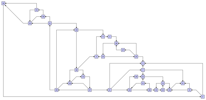
Figure 13: Example layout of a biconnected 4-planar graph. Vertices are labeled by their indices. The corresponding SPQR-tree $\mathcal{T}$ has been rooted at a Q-node representing the edge $(v_{32},v_{2})$ with the only child being an S-node whose skeleton is the simple cycle $v_{32},v_{21},v_{2}$. It has two R-nodes as children, a smaller in the upper left (with poles $\{v_{32},v_{21}\}$) and a larger one (with poles $\{v_{21},v_{2}\}$) occupying most of the drawing area. The latter one contains two smaller S-nodes (with poles $\{v_{10},v_{12}\}$ and $\{v_{4},v_{26}\}$) and a P-node (with poles $\{v_{26},v_{25}\}$) that has two children. One of them being an $(s,t)$-edge, the other one an S-node.

Drawing edges as octilinear paths plays a central role in the design of metro-maps (see e.g., [8, 17, 18]), which dates back to the 1930’s when Henry Beck, an engineering draftsman, designed the first schematic map of London Underground using mostly horizontal, vertical and diagonal segments; see Fig.1. Laying out networks in such a way is called octilinear graph drawing. More precisely, an octilinear drawing of a (planar) graph $G=(V,E)$ of maximum degree eight is a (planar) drawing $\Gamma(G)$ of $G$ in which each vertex occupies a point on the integer grid and each edge is drawn as a sequence of alternating horizontal, vertical and diagonal ($45^{\circ}$) line-segments. For an example, see Fig.13 in Section 7.

Figure 1: Henry Beck Tube Map (first edition), 1933. Printed at Waterlow & Sons Ltd., London.

For drawings of (planar) graphs to be readable, special care is needed to keep the number of bends small. However, the problem of determining whether a given embedded 8-planar graph (that is, a planar graph of maximum degree eight with given combinatorial embedding) admits a bendless octilinear drawing is NP-hard [16]. This negative result motivated us to study octilinear drawings of low edge complexity, that is, with few bends per edge. Surprisingly enough, very few results relevant to this problem were known, even if the octilinear model has been well-studied in the context of metro-map visualization and map schematization (see e.g. [20]). As an immediate byproduct of a result of Keszegh et al. [12], it turns out that every $d$-planar graph, with $3\leq d\leq 8$, admits a planar octilinear drawing with at most two bends per edge; see Section 2. On the other hand, every 3-planar graph on five or more vertices admits a planar octilinear drawing in which all edges are bendless [5, 11].

In this paper, we bridge the gap between the two aforementioned results. In particular, we prove that every 4-planar graph admits a planar octilinear drawing with at most one bend per edge in cubic area (see Section 4). We further show that every 5-planar graph also admits a planar octilinear drawing with at most one bend per edge, but our construction may require super-polynomial area (see Section 5). Hence, we have made no effort in proving a concrete bound. We complement our results by demonstrating an infinite class of 6-planar graphs whose planar octilinear drawings require at least two bends per edge (see Section 6).

2 Related Work

The research on the (planar) slope number of graphs focuses on minimizing the number of used slopes (see e.g., [9, 12, 13, 14, 15]). Octilinear drawings can be seen as a special case thereof, since only four slopes (horizontal, vertical and the two diagonals) are used. In a related work, Keszegh et al. [12] showed that any $d$-planar graph admits a planar drawing with one bend per edge, in which all edge-segments have at most $2d$ different slopes. So, for $d=4$ and for $d=5$, we significantly reduce the number of different slopes from $8$ and $10$, resp., to $4$. They also proved that $d$-planar graphs, with $d\geq 3$, admit planar drawings with two bends per edge that require at most $\lceil\frac{d}{2}\rceil$ different slopes. It is not difficult to transfer this technique to the octilinear model and show that any $d$-planar graph, with $3\leq d\leq 8$, admits a planar octilinear drawing with two bends per edge. However, for $d=3$, Di Giacomo et al. [5] recently proved that any 3-planar graph with $n\geq 5$ vertices has a bendless planar drawing with at most $4$ different slopes and angular resolution $\pi/4$ (see also [11]); their approach also yields octilinear drawings.

Octilinear drawings can be considered as an extension of orthogonal drawings, which allow only horizontal and vertical segments (i.e., graphs of maximum degree $4$ admit such drawings). Tamassia [19] showed that one can minimize the total number of bends in orthogonal drawings of embedded 4-planar graphs. However, minimizing the number of bends over all embeddings of a 4-planar graph is NP-hard [6]. Note that the core of Tamassia’s approach is a min-cost flow algorithm that first specifies the angles and the bends of the drawing, producing an orthogonal representation, and then based on this representation computes the actual drawing by specifying the exact coordinates for the vertices and the bends of the edges. It is known that Tamassia’s algorithm can be employed to produce a bend-minimum octilinear representation for any given embedded 8-planar graph. However, a bend-minimum octilinear representation may not be realizable by a corresponding planar octilinear drawing [3]. Furthermore, the number of bends on a single edge might be very high, but can easily be bounded by applying appropriate capacity constraints to the flow-network.

Biedl and Kant [1] showed that any 4-planar graph except the octahedron admits a planar orthogonal drawing with at most two bends per edge on an $O(n^{2})$ integer grid. Hence, the octilinear drawing model allows us to reduce the number of bends per edge at the cost of an increased area. On the other hand, not all 4-planar graphs admit orthogonal drawings with one bend per edge; however, testing whether a 4-planar graph admits such a drawing can be done in polynomial time [2]. In the context of metro-map visualization, several approaches have been proposed to produce metro-maps using octilinear or nearly-octilinear polylines, such as force-driven algorithms [8], hill climbing multi-criteria optimization techniques [18] and mixed-integer linear programs [17]. However, the problem of laying out a metro-map in an octilinear fashion is significantly more difficult than the octilinear graph drawing problem, as several metro-lines may connect the same pair of stations and the positions of the vertices have to reflect geographical coordinates of the stations.

3 Preliminaries

In our algorithms, we incrementally construct the drawings similar to the method of Kant [10]. We first employ the canonical order to cope with triconnected graphs. Then, we extend them to biconnected graphs using the SPQR-tree [4] and to simply connected graphs using the BC-tree. In this section we briefly recall them; however we assume basic familiarity.

Definition 1 (Canonical order [10]).

For a given triconnected plane graph $G=(V,E)$ let $\Pi=(P_{0},\ldots,P_{m})$ be a partition of $V$ into paths such that $P_{0}=\{v_{1},v_{2}\}$, $P_{m}=\{v_{n}\}$ and $v_{2}\rightarrow v_{1}\rightarrow v_{n}$ is a path on the outer face of $G$. For $k=0,\ldots,m$ let $G_{k}$ be the subgraph induced by $\cup_{i=0}^{k}P_{i}$ and assume it inherits its embedding from $G$. Partition $\Pi$ is a canonical order of $G$ if for each $k=1,\ldots,m-1$ the following hold: (i) $G_{k}$is biconnected, (ii) all neighbors of $P_{k}$ in $G_{k-1}$ are on the outer face, of $G_{k-1}$ (iii) all vertices of $P_{k}$ have at least one neighbor in $P_{j}$ for some $j>k$. $P_{k}$ is called a singleton if $|P_{k}|=1$ and a chain otherwise.

Definition 2 (BC-tree).

The BC-tree $\mathcal{B}$ of a connected graph $G$ has a B-node for each biconnected component of $G$ and a C-node for each cutvertex of $G$. Each B-node is connected with the C-nodes that are part of its biconnected component.

An SPQR-tree [4] provides information about the decomposition of a biconnected graph into its triconnected components. It can be computed in linear time and space [7]. Every triconnected component is associated with a node $\mu$ in the SPQR-tree $\mathcal{T}$. The triconnected component itself is referred to as the skeleton of $\mu$, denoted by $G^{\textit{skel}}_{\mu}=(V^{\textit{skel}}_{\mu},E^{\textit{skel}}_{\mu})$. We refer to the degree of a vertex $v\in V^{\textit{skel}}_{\mu}$ in $G^{\textit{skel}}_{\mu}$ as $\textit{deg}^{\textit{skel}}_{\mu}(v)$. We say that $\mu$ is an R-node, if $G^{\textit{skel}}_{\mu}$ is a simple triconnected graph. A bundle of at least three parallel edges classifies $\mu$ as a P-node, while a simple cycle of length at least three classifies $\mu$ as an S-node. By construction R-nodes are the only nodes of the same type that are allowed to be adjacent in $\mathcal{T}$. The leaves of $\mathcal{T}$ are formed by the Q-nodes. Their skeleton consists of two parallel edges; one of them corresponds to an edge of $G$ and is referred to as real edge. The skeleton edges that are not real are referred to as virtual edges. A virtual edge $e$ in $G^{\textit{skel}}_{\mu}$ corresponds to a tree node $\mu^{\prime}$ that is adjacent to $\mu$ in $\mathcal{T}$, more exactly, to another virtual edge $e^{\prime}$ in $G^{\textit{skel}}_{\mu^{\prime}}$. We assume that $\mathcal{T}$ is rooted at a Q-node. Hence, every skeleton (except the one of the root) contains exactly one virtual edge $e=(s,t)$ that has a counterpart in the skeleton of the parent node. We call this edge the reference edge of $\mu$ denoted by $\textit{ref}(\mu)$. Its endpoints, $s$ and $t$, are named the poles of $\mu$ denoted by $\mathcal{P}_{\mu}=\{s,t\}$. Every subtree rooted at a node $\mu$ of $\mathcal{T}$ induces a subgraph of $G$ called the pertinent graph of $\mu$ that we denote by $G^{\textit{pert}}_{\mu}=(V^{\textit{pert}}_{\mu},E^{\textit{pert}}_{\mu})$. We abbreviate the degree of a node $v$ in $G^{\textit{pert}}_{\mu}$ with $\textit{deg}^{\textit{pert}}_{\mu}(v)$. The pertinent graph is the subgraph of $G$ for which the subtree describes the decomposition.

Now, assume that $G$ be a simple, biconnected $k$-planar graph, whose SPQR-tree $\mathcal{T}$ is given. Additionally, we may assume that $\mathcal{T}$ is rooted at a Q-node that is adjacent to an S- or R-node. Notice that at least one such node exists since the graph does not contain any multi-edges, which would be the case if only a P-node existed. Biconnectivity and maximum degree of $k$ yield basic bounds for the graph degree of a node $v\in V$, i.e., $2\leq\textit{deg}(v)\leq k$. By construction the pertinent graph of a tree node $\mu$ is a (connected) subgraph of $G$; thus $1\leq\textit{deg}^{\textit{pert}}_{\mu}(v)\leq\textit{deg}(v)$. For the degrees in a skeleton graph $G^{\textit{skel}}_{\mu}$, we obtain bounds based on the type of the corresponding node. Skeletons of Q-nodes are cycles of length two, whereas S-nodes are by definition simple cycles of length at least three; hence, $\textit{deg}^{\textit{skel}}_{\mu}(v)=2$. For P- and R-nodes the degree can be bounded by $3\leq\textit{deg}^{\textit{skel}}_{\mu}(v)\leq k$, since the skeleton of the former is at least a bundle of three parallel virtual edges and the latter’s skeleton is triconnected by definition. The upper bound is derived from the relation between skeleton and graph degrees: A virtual edge $e=(s,t)$ hides at least one incident edge of each node (not necessarily an $(s,t)$-edge). This observation can be easily proven by induction on the tree. Hence, $2\leq\textit{deg}^{\textit{skel}}_{\mu}(v)\leq\textit{deg}(v)$.

Next, we use this observation to derive bounds for the pertinent degree by distinguishing two cases depending on whether $v$ is a pole or not. Recall that $G^{\textit{pert}}_{\mu}$ is a subgraph of $G$ that is obtained by recursively replacing virtual edges by the skeletons of the corresponding children. In the first case when $v$ is an internal node in $G^{\textit{pert}}_{\mu}$, i.e., $v\notin\mathcal{P}_{\mu}$, $v$ is not incident to the reference edge in $G^{\textit{skel}}_{\mu}$. Thus, every edge of $G$ hidden by a virtual edge in $G^{\textit{skel}}_{\mu}$ is in $G^{\textit{pert}}_{\mu}$. Hence, $\textit{deg}^{\textit{skel}}_{\mu}(v)\leq\textit{deg}^{\textit{pert}}_{\mu}(v)\leq k$. In the other case, i.e., $v\in\mathcal{P}_{\mu}$, at least one edge that is hidden by the reference edge, is not part of $G^{\textit{pert}}_{\mu}$, thus, $\textit{deg}^{\textit{skel}}_{\mu}(v)-1\leq\textit{deg}^{\textit{pert}}_{\mu}(v)\leq k-1$. Notice that the lower bounds depend on the skeleton degree which in turn depends on the type of node, unlike the upper bounds that hold for all tree nodes. The next lemma tightens these bounds based on the type of the parent node.

Lemma 1.

Let $\mu$ be a tree node that is not the root in the SPQR-tree $\mathcal{T}$ of a simple, biconnected, $k$-planar graph $G$ and $\mu^{\prime}$ its parent in $\mathcal{T}$. For $v\in\mathcal{P}_{\mu}$, it holds that $\textit{deg}^{\textit{pert}}_{\mu}(v)\leq k-2$, if $\mu^{\prime}$ is a P- or an R-node and $\textit{deg}^{\textit{pert}}_{\mu}(v)\leq k-1$ otherwise, i.e. $\mu^{\prime}$ is an S- or a Q-node.

Proof.

Since the case where $\mu^{\prime}$ is an S- or a Q-node follows from the fact that $G$ is k-planar and the reference edge hides at least one edge that is not in $G^{\textit{pert}}_{\mu}$, we restrict ourselves to the more interesting cases where $\mu^{\prime}$ is either a P- or an R-node. From our previous observations we know that $3\leq\textit{deg}^{\textit{skel}}_{\mu^{\prime}}(v)\leq k$. Each of the at least three edges in $G^{\textit{skel}}_{\mu^{\prime}}$ hides at least one edge of $G$ that is incident to $v$. However, the total number of edges is at most $k$ due to the degree restriction. Hence, we are left with the problem of $k$ edges of $G$ being hidden by at least three virtual edges, each hiding at least one. As a result the virtual edge that corresponds to $\mu$ cannot contribute more than $k-2$ edges to its pertinent graph $G^{\textit{pert}}_{\mu}$. ∎

Lemma 2.

In the SPQR-tree $\mathcal{T}$ of a planar biconnected graph $G=(V,E)$ with $\deg(v)\geq 3$ for every $v\in V$, there exists at least one Q-node that is adjacent to a P- or an R-node.

Proof.

Assume to the contrary that all Q-nodes are adjacent to S-nodes only. We pick such a Q-node and root $\mathcal{T}$ at it. Let $\mu$ be an S-node (possibly the root itself) with poles $\mathcal{P}_{\mu}=\{s,t\}$ such that there is no other S-node in the subtree of $\mu$. By definition of an S-node, $\mu$ has at least two children. If all of them were Q-nodes then there exists a $v\in V^{\textit{skel}}_{\mu}$ with $s\neq v\neq t$ and $\deg(v)=2$; a contradiction. Hence, there is at least one child $\mu^{\prime}$ that is a P- or an R-node. However, since the leaves of $\mathcal{T}$ are Q-nodes and those are not allowed to be children of P- and R-nodes by our assumption, there exists at least one other S-node in the subtree of $\mu^{\prime}$ and therefore in the subtree of $\mu$ which contradicts our choice of $\mu$. ∎

4 Octilinear Drawings of 4-Planar Graphs

In this section, we focus on planar octilinear drawings of 4-planar graphs. We first consider the case of triconnected 4-planar graphs and then we extend our approach first to biconnected and then to simply connected graphs. Central in our approach is the port assignment; by the port of a vertex we refer to the side of the vertex an edge is connected to. The different ports on a vertex are distinguished by the cardinal directions.

4.1 The Triconnected Case

Let $G=(V,E)$ be a triconnected 4-planar graph and $\Pi=\{P_{0},\ldots,P_{m}\}$ be a canonical order of $G$. We momentarily neglect the edge $(v_{1},v_{2})$ of the first partition $P_{0}$ of $\Pi$ and we start by placing the second partition, say a chain $P_{1}=\{v_{3},\ldots, v_{|P_{1}|+2}\}$, on a horizontal line from left to right. Since by definition of $\Pi$, $v_{3}$ and $v_{|P_{1}|+2}$ are adjacent to the two vertices, $v_{1}$ and $v_{2}$, of the first partition $P_{0}$, we place $v_{1}$ to the left of $v_{3}$ and $v_{2}$ to the right of $v_{|P_{1}|+2}$. So, they form a single chain where all edges are drawn using horizontal line-segments that are attached to the east and west port at their endpoints. The case where $P_{1}$ is a singleton is analogous. Having laid out the base of our drawing, we now place in an incremental manner the remaining partitions. Assume that we have already constructed a drawing for $G_{k-1}$ and we now have to place $P_{k}$, for some $k=2,\ldots,m-1$.

In case where $P_{k}=\{v_{i},\ldots,v_{j}\}$ is a chain of $j-i+1$ vertices, we draw them from left to right along a horizontal line one unit above $G_{k-1}$. Since $v_{i}$ and $v_{j}$ are the only vertices that are adjacent to vertices in $G_{k-1}$, both only to one, we place the chain between those two as in Fig.2a. The port used at the endpoints of $P_{k}$ in $G_{k-1}$ depends on the following rule: Let $v_{i}^{\prime}$ ($v_{j}^{\prime}$, resp.) be the neighbor of $v_{i}$ ($v_{j}$, resp.) in $G_{k-1}$. If the edge $(v_{i},v_{i}^{\prime})$ ($(v_{j},v_{j}^{\prime})$, resp.) is the last to be attached to vertex $v_{i}^{\prime}$ ($v_{j}^{\prime}$, resp.), i.e., there is no vertex $v$ in $P_{l}\in\Pi$, $l>k$ such that $(v_{i}^{\prime},v)\in E$ ($(v_{j}^{\prime},v)\in E$, resp.), then we use the northern port of $v_{i}^{\prime}$ ($v_{j}^{\prime}$, resp.). Otherwise, we choose the north-east port for $(v_{i},v_{i}^{\prime})$ or the north-west port for $(v_{j},v_{j}^{\prime})$.

In case of a singleton $P_{k}=\{v_{i}\}$, we can apply the previous rule if the singleton is of degree three, as the third neighbor of $v_{i}$ should belong to a partition $\Pi_{j}$ for some $j>k$. However, in case where $v_{i}$ is of degree four we may have to deal with an additional third edge $(v_{i},v)$ that connects $v_{i}$ with $G_{k-1}$. By the placement so far, we may assume that $v$ lies between the other two endpoints, thus, we place $v_{i}$ such that $x(v_{i})=x(v)$. This enables us to draw $(v_{i},v)$ as a vertical line-segment; see Fig.2b.

The above procedure is able to handle all chains and singletons except the last partition $P_{m}$, because $v_{n}$ may have $4$ edges pointing downwards. One of these edges is $(v_{n},v_{1})$, by definition of $\Pi$. We exclude $(v_{n},v_{1})$ and draw $v_{n}$ as an ordinary singleton. Then, we shift $v_{1}$ to the left and up as in Fig.2c. This enables us to draw $(v_{1},v_{n})$ as a horizontal-vertical segment combination. For $(v_{1},v_{2})$, we move $v_{2}$ one unit to the right and down. We free the west port of $v_{2}$ by redrawing its incident edges as in Fig.2c and attach $(v_{1},v_{2})$ to it. Edge $(v_{1},v_{2})$ will be drawn as a diagonal segment with positive slope connected to $v_{1}$ and a horizontal segment connected to $v_{2}$, which requires one bend. Let $(v_{2},v_{i})$ be the other incomplete edge according to Figure 2c. It will be drawn using a diagonal segment with positive slope connected to $v_{2}$ and a horizontal segment connected to $v_{i}$, again requiring one bend.

So far, we have specified a valid port assignment and the y-coordinates of the vertices. However, we have not fully specified their x-coordinates. Notice that by construction every edge, except the ones drawn as vertical line-segments, contains exactly one horizontal segment. This enables us to stretch the drawing horizontally by employing appropriate cuts. A cut, for us, is a $y$-monotone continuous curve that crosses only horizontal segments and divides the current drawing into a left and a right part. It is not difficult to see that we can shift the right part of the drawing that is defined by the cut further to the right while keeping the left part of the drawing on place and the result remains a valid octilinear drawing.

To compute the x-coordinates, we proceed as follows. We first assign consecutive x-coordinates to the first two partitions and from there on we may have to stretch the drawing in two cases. The first one appears when we introduce a chain, say $P_{k}$, as it may not fit into the gap defined by its two adjacent vertices in $G_{k-1}$. In this case, we horizontally stretch the drawing between its two adjacent vertices in $G_{k-1}$ to ensure that their horizontal distance is at least $|P_{k}|+1$. The other case appears when an edge that contains a diagonal segment is to be drawn. Such an edge requires a horizontal distance between its endpoints that is at least the height it bridges. We also have to prevent it from intersecting any horizontal-vertical combinations in the face below it. We can cope with both cases by horizontally stretching the drawing by a factor that is bounded by the current height of the drawing. Since the height of the resulting drawing is bounded by $|\Pi|=O(n)$, it follows that in the worst case its width is $O(n^{2})$. We are now ready to state the main theorem of this subsection.

(a)

(b)

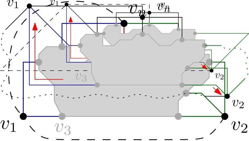
(c)

Figure 2: (a) Horizontal placement of a chain $P_{k}=\{v_{i},\ldots,v_{j}\}$. (b) Placement of a singleton $P_{k}=\{v_{i}\}$ with degree four. (c) Final layout after repositioning $v_{1}$ and $v_{2}$ (the shape of the dotted edges can be obtained by extending the stubs until they intersect).

Theorem 1.

Given a triconnected 4-planar graph $G$, we can compute in $O(n)$ time an octilinear drawing of $G$ with at most one bend per edge on an $O(n^{2})\times O(n)$ integer grid.

Proof.

In order to keep the time complexity of our algorithm linear, we employ a simple trick. We assume that any two adjacent points of the underlying integer grid are by $n$ units apart in the horizontal direction and by one unit in the vertical direction. This a priori ensures that all edges that contain a diagonal segment will not be involved in crossings and simultaneously does not affect the total area of the drawing, which asymptotically remains cubic. On the other hand, the advantage of this approach is that we can use the shifting method of Kant [10] to cope with the introduction of chains in the drawing, that needs $O(n)$ time in total by keeping relative coordinates that can be efficiently updated and computing the absolute values only at the last step. ∎

Note that our algorithm produces drawings that have a linear number of bends in total (in particular, exactly $2|\Pi|=O(n)$ bends). In the following, we prove that this bound is asymptotically tight.

Theorem 2.

There exists an infinite class of 4-planar graphs which do not admit bendless octilinear drawings and if they are drawn with at most one bend per edge, then a linear number of bends is required.

Proof.

Based on the simple fact that in an orthogonal drawing a triangle requires at least one bend, we describe an example that translates this idea to the octilinear model (see Fig.3). While a triangle can easily be drawn bendless with the additional ports available, we will occupy those to enforce the creation of a bend as in the orthogonal model. Furthermore, the example is triconnected. Hence, its embedding is fixed up to the choice of the outer face. Our construction is heavily based on the so called separating triangle, i.e., a three-cycle whose removal disconnects the graph. Each vertex of such a triangle has degree four. Any triangle which is drawn bendless has a $45^{\circ}$ angle inside. But since the triangles are nested and have incident edges going inside of the triangles, this is impossible. ∎

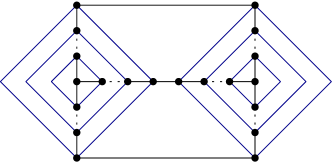
Figure 3: Nested separating triangles each requiring one bend.

4.2 The Biconnected Case

Following standard practice, we employ a rooted SPQR-tree and assume for a tree node that the pertinent graphs of its children are drawn in a pre-specified way. Consider a node $\mu$ in $\mathcal{T}$ with poles $\mathcal{P}_{\mu}=\{s,t\}$. In the drawing of $G^{\textit{pert}}_{\mu}$, $s$ should be located at the upper-left and $t$ at the lower-right corner of the drawing’s bounding box with a port assignment as in Fig.4a. In general, we assume that the edges incident to $s$ ($t$, resp.) use the western (eastern, resp.) port at their other endpoint, except of the northern (southern, resp.) most edge which may use the north (south, resp.) port instead. In that case we refer to $s$ and $t$ as fixed; see $\overline{e}_{s},\overline{e}_{t}$ in Fig.4a. More specifically, we maintain the following invariants:

1. The width (height) of the drawing of $\mu$ is quadratic (linear) in the size of $G^{\textit{pert}}_{\mu}$. $s$ is located at the upper-left; $t$ at the lower-right corner of the drawing’s bounding box.

2. If $\textit{deg}^{\textit{pert}}_{\mu}(s)\geq 2$, $s$ is fixed; $t$ is fixed if $\textit{deg}^{\textit{pert}}_{\mu}(t)=3$ and $\mu$’s parent is not the root.

3. The edges that are incident at $s$ and $t$ in $G^{\textit{pert}}_{\mu}$ use the south, south-east and east ports at $s$ and the north, north-west and west port at $t$, resp. If $s$ or $t$ is not fixed, incident edges are attached at their other endpoints via the west and east port, respectively. If $s$ or $t$ is fixed, the northern-most edge at $s$ and the southern-most edge at $t$ may use the north (south, resp.) port at its other endpoint.

Notice that the port assignment, i.e. IP-3, guarantees the ability to stretch the drawing horizontally even in the case where both poles are fixed. Furthermore, IP-2 is interchangeable in the following sense: If $\textit{deg}^{\textit{pert}}_{\mu}(s)=2$ and $\textit{deg}^{\textit{pert}}_{\mu}(t)=1$, then $s$ is fixed but $t$ is not. But, if we relabel $s$ and $t$ such that $t^{\prime}=s$ and $s^{\prime}=t$, then $\textit{deg}^{\textit{pert}}_{\mu}(s^{\prime})=1$ and $\textit{deg}^{\textit{pert}}_{\mu}(t^{\prime})=2$. By IP-2, we can create a drawing where both $s^{\prime}$ and $t^{\prime}$ are not fixed and located in the upper-left and lower-right corner of the drawing’s bounding box. Afterwards, we mirror the resulting layout vertically and horizontally to obtain one where $s$ and $t$ are in their respective corners and not fixed. Notice that in general the property of being fixed is not symmetric, e.g., when $\textit{deg}^{\textit{pert}}_{\mu}(s)=3$ and $\textit{deg}^{\textit{pert}}_{\mu}(t)=2$ holds, $s$ remains fixed while $t$ becomes fixed as well. For a non-fixed vertex, we introduce an operation that is referred to as forming or creating a nose; see Fig.4b, where $t$ has been moved downwards at the cost of a bend. As a result, the west port of $t$ is no longer occupied.

(a)

(b)

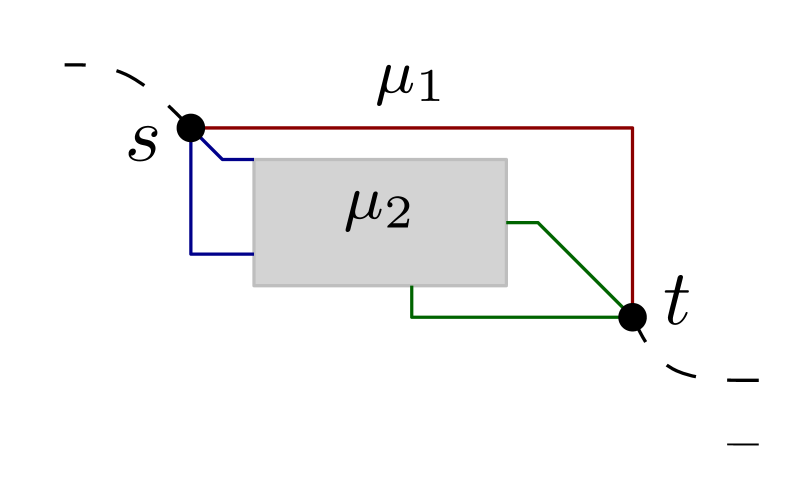
(c)

(d)

Figure 4: (a) Schematic view of the layout requirements. (b) Creating a nose at $t$. (c) First P-node subcase without an $(s,t)$-edge but $s$ might be fixed in a child $\mu_{1}$. (d) Second P-node subcase with an $(s,t)$-edge where $t$ might get fixed in a child $\mu_{2}$.

P-node case:

Let $\mu$ be a P-node. By Lemma 1, for a child $\mu^{\prime}$ of $\mu$, it holds that $\textit{deg}^{\textit{pert}}_{\mu^{\prime}}(s)\leq 2$ and $\textit{deg}^{\textit{pert}}_{\mu^{\prime}}(t)\leq 2$. So, $t$ can form a nose in $\mu^{\prime}$, while $s$ might be fixed in the case where $\textit{deg}^{\textit{pert}}_{\mu^{\prime}}(s)=2$. Notice that there exists at most one such child due to the degree restriction. We distinguish two cases based on the existence of an $(s,t)$-edge.

In the first case, assume that there is no $(s,t)$-edge, i.e., there is no child that is a Q-node. We draw the children of $\mu$ from top to bottom such that a possible child in which $s$ is fixed, is drawn topmost (see $\mu_{1}$ in Fig.4c). In the second case, we draw the $(s,t)$-edge at the top and afterwards the remaining children (see Fig.4d). Of course, this works only if $s$ is not fixed in any of the other children. Let $\mu^{\prime}$ be such a potential child where $s$ is fixed, i.e., $\textit{deg}^{\textit{pert}}_{\mu^{\prime}}(s)=2$, and thus, the only child that remains to be drawn. Here, we use the property of interchangeability to “unfix” $s$ in $\mu^{\prime}$. As a result $s$ can form a nose, whereas $t$ may now be fixed in $\mu^{\prime}$ when $\textit{deg}^{\textit{pert}}_{\mu^{\prime}}(t)=2$ holds, as in Fig.4d. However, then $\textit{deg}^{\textit{pert}}_{\mu}(t)=3$ follows. Notice that the presence of an $(s,t)$-edge implies that the parent of $\mu$ is not the root of $\mathcal{T}$, since this would induce a pair of parallel edges. Hence, by IP-2 we are allowed to fix $t$ in $\mu$. Port assignment and area requirements comply in both cases with our invariant properties.

S-node case:

We place the drawings of the children, say $\mu_{1},\ldots,\mu_{\ell}$, of an S-node $\mu$ in a “diagonal manner” such that their corners touch as in Fig.5a. In case of Q-nodes being involved, we draw their edges as horizontal segments (see, e.g., edge $(v_{3},v_{4})$ in Fig.5a that corresponds to Q-node $\mu_{3}$). Observe that $s$ and $t$ inherit their port assignment and pertinent degree from $\mu_{1}$ and $\mu_{\ell}$, respectively, i.e., $\textit{deg}^{\textit{pert}}_{\mu}(s)=\textit{deg}^{\textit{pert}}_{\mu_{1}}(s)$ and $\textit{deg}^{\textit{pert}}_{\mu}(t)=\textit{deg}^{\textit{pert}}_{\mu_{\ell}}(t)$. So, we may assume that $s$ is fixed in $\mu$, if $s$ is fixed in $\mu_{1}$. Similarly, $t$ is fixed in $\mu$, if $t$ is fixed in $\mu_{\ell}$. By IP-2, $t$ is not allowed to be fixed in the case where the parent of $\mu$ is the root of $\mathcal{T}$. However, Lemma 2 states that we can choose the root such that $t$ is not fixed in that case, and thus, complies with IP-2. Since we only concatenated the drawings of the children, IP-1 and IP-3 are satisfied.

R-node case:

For the case where $\mu$ is an R-node with poles $\mathcal{P}_{\mu}=\{s,t\}$, we follow the basic idea of the triconnected algorithm of the previous section and describe the modifications necessary to handle the drawing of the children of $\mu$. To do so, we assume the worst case where no child of $\mu$ is a Q-node. Let $\mu_{uv}$ denote the child that is represented by the virtual edge $(u,v)\in E^{\textit{skel}}_{\mu}$. Notice that due to Lemma 1, $\textit{deg}^{\textit{pert}}_{\mu_{uv}}(u)\leq 2$ and $\textit{deg}^{\textit{pert}}_{\mu_{uv}}(v)\leq 2$ holds. Hence, with IP-2 we may assume that at most one out of $u$ and $v$ is fixed in $\mu_{uv}$. We choose the first partition in the canonical ordering to be $P_{0}=\{s,t\}$ and distinguish again between whether the partition to be placed next is a chain or a singleton.

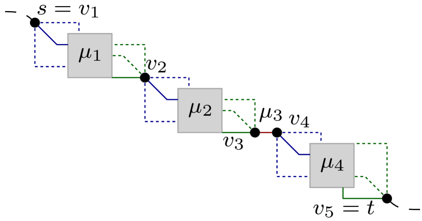
(a)

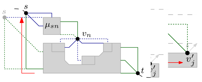
(b)

(c)

(d)

Figure 5: (a) S-node with children $\mu_{1},\ldots,\mu_{4}$; $\mu_{3}$ is a Q-node representing the edge $(v_{3},v_{4})$. Optional edges are drawn dotted. (b) Example for a chain $v_{i},\ldots,v_{j}$ with virtual edges representing $\mu_{i},\ldots,\mu_{j-1}$ in the R-node case. (c) Singleton $v_{i}$ with possibly three incident virtual edges representing $\mu^{\prime}_{i},\mu^{\prime}_{v},\mu^{\prime}_{j}$. (d) Placing $v_{n}$ and moving up $s$ which might be fixed in $\mu_{sn}$.

In case of a chain, say $P_{k}=\{v_{i},\ldots,v_{j}\}$ with two neighbors $v_{i}^{\prime}$ and $v_{j}^{\prime}$ in $G_{k-1}$, we have to replace two types of edges with the drawings of the corresponding children: the edges $(v_{i},v_{i+1}),\ldots,(v_{j-1},v_{j})$ representing the children $\mu_{i},\ldots,\mu_{j-1}$ and $(v_{i}^{\prime},v_{i})$ ($(v_{j},v_{j}^{\prime})$ resp.) representing $\mu_{i}^{\prime}$ ($\mu_{j}^{\prime}$ resp.). We place the vertices of $P_{k}$ on a horizontal line high enough above $G_{k-1}$ such that every drawing may fit in-between it and $G_{k-1}$. Then, we insert the drawings aligned below the horizontal line and choose for $i\leq l<j$, $v_{l}$ to be the fixed node in $\mu_{l}$, whereas in $\mu_{i}^{\prime}$ ($\mu_{j}^{\prime}$ resp.), we set $v_{i}$ ($v_{j}$ resp.) to be fixed. Hence, for $i\leq l<j$, $v_{l+1}$ may form a nose in $\mu_{l}$ pointing upwards while $v_{i}^{\prime}$ and $v_{j}^{\prime}$ form each one downwards as depicted in Fig.5b. For the extra height and width, we stretch the drawing horizontally.

For the case where $P_{k}=\{v_{i}\}$ and $i\neq n$ is a singleton, we only outline the difference which is a possible third edge $(v_{i},v)$ to $G_{k-1}$ representing say $\mu_{v}^{\prime}$. While the other two involved children, say $\mu_{i}^{\prime}$ and $\mu_{j}^{\prime}$, are handled as in the chain-case, $\mu_{v}^{\prime}$ requires extra height now and we may place $v_{i}$ such that $\mu_{v}^{\prime}$ fits below $\mu_{j}^{\prime}$ as in Fig.5c. Notice that $\textit{deg}^{\textit{pert}}_{\mu_{v}^{\prime}}(v_{i})=1$ holds and therefore by IP-2 both $v_{i}$ and $v$ are not fixed in $\mu_{v}^{\prime}$. Hence, forming a nose at $v_{i}$ and $v$ as in Fig.5c is feasible.

It remains to describe the special case where the last singleton $P_{k}=\{v_{n}\}$ is placed. Since $s,t\in P_{0}$, both have not been fixed yet. We proceed as in the triconnected algorithm and move $s=v_{1}$ above $v_{n}$ as depicted in Fig.5d, high enough to accommodate the drawing of the child $\mu_{sn}$ represented by the edge $(s,v_{n})$. Since we may require $v_{n}$ to form a nose in $\mu_{sn}$ as in Fig.5d, we choose $s$ to be fixed in $\mu_{sn}$. However, we are allowed by IP-2 to fix $s$ since $t$ remains unfixed. For the area constraints of IP-1, we argue as follows: Although some diagonal segments may force us to stretch the whole drawing by its height, the height of the drawing has been kept linear in the size of $G^{\textit{pert}}_{\mu}$. Since we increase the width by the height a constant number of times per step, the resulting width remains quadratic.

Root case:

For the root of $\mathcal{T}$ we distinguish two cases: In the first case, there exists a vertex $v\in V$ with $\deg(v)\leq 3$. Then, we choose as root a Q-node $\mu$ that represents one of its three incident edges and orient the poles $\{s,t\}$ such that $t=v$. Hence, for the child $\mu^{\prime}$ of $\mu$ follows $\textit{deg}^{\textit{pert}}_{\mu^{\prime}}(t)\leq 2$. In the other case, i.e., for every $v\in V$ we have $\deg(v)=4$, we choose a Q-node that is not adjacent to an S-node, whose existence is guaranteed by Lemma 2. In both cases, we may form a nose with $t$ pointing downwards and draw the edge as in the triconnected algorithm.

Theorem 3.

Given a biconnected 4-planar graph $G$, we can compute in $O(n)$ time an octilinear drawing of $G$ with at most one bend per edge on an $O(n^{2})\times O(n)$ integer grid.

Proof.

The SPQR-tree $\mathcal{T}$ can be computed in $O(n)$-time and its size is linear to the size of $G$ [7]. The pertinent degrees of the poles at every node can be pre-computed by a bottom-up traversal of $\mathcal{T}$. Drawing a P-node requires constant time; S- and R-nodes require time linear to the size of the skeleton. However, the sum over all skeleton edges is linear, as every virtual edge corresponds to a tree node. ∎

4.3 The Simply Connected Case

After having shown that we can cope with biconnected 4-planar graphs, we turn our attention to the connected case. We start by computing the BC-tree of $G$ and root it at some arbitrary B-node. Every B-node, except the root, contains a designated cut vertex that links it to the parent. A bridge for a biconnected component consists only of a single edge. Similar to the biconnected case, we define an invariant for the drawing of a subtree: The cut vertex that links the subtree to the parent is located in the upper left corner of the drawing’s bounding box.

(a)

(b)

(c)

(d)

Figure 6: (a) Rooting the SPQR-tree such that $v_{b}$ is in the upper-left corner. (b) All possible situations at an S-node $\mu$. For attaching $b_{2}$ to $v_{2}$, the layout had to be modified. (c) Attaching a subtree via a bridge to a cut vertex $v_{c}$ in an R-node. The dashed edge $(v_{i},v^{\prime})$ may only be present if $v_{i}=v_{n}$. (d) A cut vertex where all of its children are attached via bridges.

Any subgraph, say $G_{b}$, induced by a non-bridge biconnected component can be laid out using the biconnected algorithm. However, to construct a drawing that satisfies our invariant we have to take care of two problems. First, the cut vertex, say $v_{b}$, that links $G_{b}$ to the parent, has to be drawn in the upper-left corner of the subtrees drawing. Second, there may be other cut vertices of $G$ in $G_{b}$ to which we have to attach their corresponding subtrees.

For the first problem we describe how to root the SPQR-tree $\mathcal{T}_{b}$ for $G_{b}$ so that $v_{b}$ is located in the upper-left corner. There are at least two Q-nodes having $v_{b}$ as a pole (as $G_{b}$ is biconnected) and the degree of $v_{b}$ in $G_{b}$ is at most $3$. In the biconnected case, we distinguished for the root of the tree between whether there exists $v\in V$ with $\deg(v)\leq 3$ or not. Hence, we may choose for the root of $\mathcal{T}_{b}$ a Q-node having $v_{b}$ as a pole and orient it such that $v_{b}=t$, thus, satisfying $\deg(t)\leq 3$. Then, we flip the final drawing of $G_{b}$ such that $t$ is in the upper left corner (see Fig.6a).

Next, we address the second problem. Let $v_{c}$ be a cut vertex in $G_{b}$ that is not the link to the parent. If $v_{c}$ has degree $3$, then it may occur in the pertinent graph of every node. However, in this case we only have to attach a subtree of the BC-tree that is connected via a bridge. This poses no problem, as there are enough free ports available at $v_{c}$ and we can afford a bend at the bridge. We only consider S- and R- nodes here since the poles of P-nodes occur in the pertinent graphs of the first two. For R-nodes we assume that the south east port at $v_{c}$ is free. So, we attach the drawing via the bridge by creating a bend as in Fig.6c. In the diagonal drawing of an S-node, the north-east port is free. So, we can proceed similar; see Fig.6b.

If $v_{c}$ has degree $2$ in $G_{b}$, it only occurs in the pertinent graph of an S-node; see $v_{3}$ in Fig.6b. However, we may no longer assume that the bridge is available. As a result, we cannot afford a bend and have to deal with two incident edges instead of one. We modify the drawing by exploiting the two real edges incident to $v_{c}$ in the S-nodes layout to free the east and south east port; see $v_{2}$ in Fig.6b. This enables us to attach the subtrees drawing without modifying it. We finish this section by dealing with the most simple case where there are only bridges attached to a cut vertex. The idea is illustrated in Fig.6d and matches our layout specification.

Theorem 4.

Given a connected 4-planar graph $G$, we can compute in $O(n)$ time an octilinear drawing of $G$ with at most one bend per edge on an $O(n^{2})\times O(n)$ integer grid.

Proof.

Decomposing a connected graph into its biconnected components takes linear time. It remains the area property. Inserting a subtree with $n$ vertices and the given dimensions into the drawing of an R- or S-node clearly increases the width of the drawing by at most $O(n^{2})$ and the height by at most $O(n)$. Hence, the total drawing area is cubic, as desired. ∎

5 Octilinear Drawings of 5-Planar Graphs

In this section, we focus on planar octilinear drawings of 5-planar graphs. As in Section 4, we first consider the case of triconnected 5-planar graphs and then we extend our approach first to biconnected and then to the simply connected graphs.

5.1 The Triconnected Case

Let $G=(V,E)$ be a triconnected 5-planar graph and $\Pi=\{P_{0},\ldots,P_{m}\}$ be a canonical order of $G$. We place the first two partitions $P_{0}$ and $P_{1}$ of $\Pi$, similar to the case of 4-planar graphs. Again, we assume that we have already constructed a drawing for $G_{k-1}$ and now we have to place $P_{k}$, for some $k=2,\ldots,m-1$. We further assume that the $x$- and $y$-coordinates are computed simultaneously so that the drawing of $G_{k-1}$ is planar and horizontally stretchable in the following sense: If $e\in E(G_{k-1})$ is an edge incident to the outer face of $G_{k-1}$, then there is always a cut which crosses $e$ and can be utilized to horizontally stretch the drawing of $G_{k-1}$. This is guaranteed by our construction which makes sure that in each step the edges incident to the outer face have a horizontal segment. In other words, one can define a cut through every edge incident to the outer face of $G_{k-1}$ (stretchability-invariant).

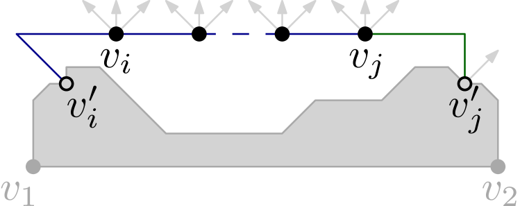
(a)

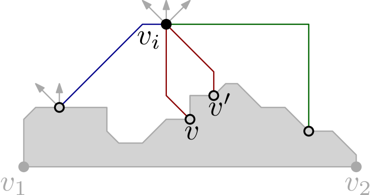
(b)

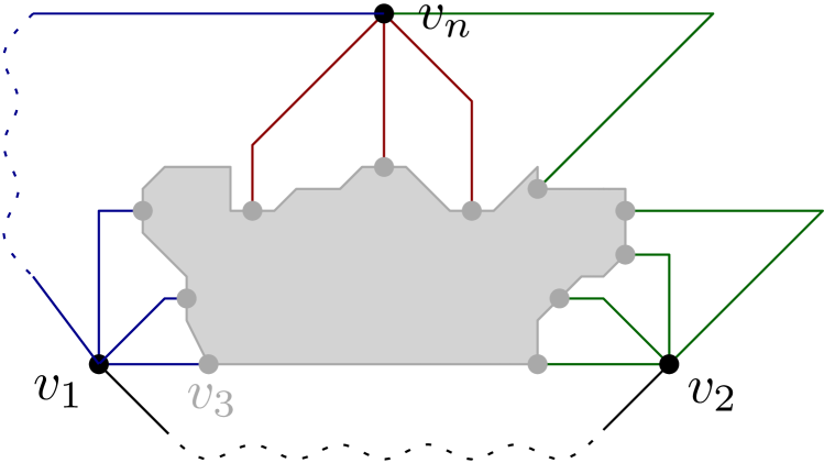
(c)

Figure 7: (a) Horizontal placement of a chain $P_{k}=\{v_{i},\ldots,v_{j}\}$. (b) Placement of a singleton $P_{k}=\{v_{i}\}$ of degree five. (c) Final layout (the shape of the dotted edges can be obtained by extending the stubs until they intersect).

If $P_{k}=\left\{v_{i},\ldots,v_{j}\right\}$ is a chain, it is placed exactly as in the case of 4-planar graphs, but with different port assignment. Recall that by $v_{i}^{\prime}$ ($v_{j}^{\prime}$, resp.) we denote the neighbor of $v_{i}$ ($v_{j}$, resp.) in $G_{k-1}$. Among the northern available ports of vertex $v_{i}^{\prime}$ ($v_{j}^{\prime}$, resp.), edge $(v_{i},v_{i}^{\prime})$ ($(v_{j},v_{j}^{\prime})$, resp.) uses the eastern-most unoccupied port of $v_{i}^{\prime}$ (western-most unoccupied port of $v_{j}^{\prime}$, resp.); see Fig.7a. If $P_{k}$ does not fit into the gap between its two adjacent vertices $v_{i}^{\prime}$ and $v_{j}^{\prime}$ in $G_{k-1}$, then we horizontally stretch $G_{k-1}$ between $v_{i}^{\prime}$ and $v_{j}^{\prime}$ to ensure that the horizontal distance between $v_{i}^{\prime}$ and $v_{j}^{\prime}$ is at least $|P_{k}|+1$. This can always be accomplished due to the stretchability-invariant, as both $v_{i}^{\prime}$ and $v_{j}^{\prime}$ are on the outer face of $G_{k-1}$. Potential crossings introduced by edges of $P_{k}$ containing diagonal segments can be eliminated by employing similar cuts to the ones presented in the case of 4-planar graphs. So, we may assume that $G_{k}$ is plane. Also, $G_{k}$ complies with the stretchability-invariant, as one can define a cut that crosses any of the newly inserted edges of $P_{k}$ and then follows one of the cuts of $G_{k-1}$ that crosses an edge between $v_{i}^{\prime}$ and $v_{j}^{\prime}$.

In case of a singleton $P_{k}=\{v_{i}\}$ of degree $3$ or $4$, our approach is very similar to the one of the case of 4-planar graphs. Here, we mostly focus on the case where $v_{i}$ is of degree five. In this case, we have to deal with two additional edges (called nested) that connect $v_{i}$ with $G_{k-1}$, say $(v_{i},v)$ and $(v_{i},v^{\prime})$; see Fig.7b. Such a pair of edges does not always allow vertex $v_{i}$ to be placed along the next available horizontal grid line; $v_{i}$’s position is more or less prescribed, as each of $v$ and $v^{\prime}$ may have only one northern port unoccupied. However, a careful case analysis on the type of ports (i.e., north-west, north or north-east) that are unoccupied at $v$ and $v^{\prime}$ in conjunction with the fact that $G_{k-1}$ is horizontally stretchable shows that we can always find a feasible placement for $v_{i}$ (usually far apart from $G_{k-1}$). Potential crossings due to the remaining edges incident to $v_{i}$ are eliminated by employing similar cuts to the ones presented in the case of 4-planar graphs. So, we may assume that $G_{k}$ is planar. Similar to the case of a chain, we prove that $G_{k}$ complies with the stretchability-invariant. In this case special attention should be paid to avoid crossings with the nested edges of $v_{i}$, as a nested edge may contain no horizontal segment. Note that the case of the last partition $P_{m}=\{v_{n}\}$ is treated in the same way, even if $v_{n}$ is potentially incident to three nested edges; see Fig.7c.

To complete the description of our approach it remains to describe how edge $(v_{1},v_{2})$ is drawn. By construction both $v_{1}$ and $v_{2}$ are along a common horizontal line. So, $(v_{1},v_{2})$ can be drawn using two diagonal segments that form a bend pointing downwards; see Fig.7c.

Theorem 5.

Given a triconnected 5-planar graph $G$, we can compute in $O(n^{2})$ time an octilinear drawing of $G$ with at most one bend per edge.

Proof.

Unfortunately, we can no longer use the shifting method of Kant [10], since the $x$- and $y$-coordinates are not independent. However, the computation of each cut can be done in linear time, which implies that our drawing algorithm needs $O(n^{2})$ time in total. ∎

Recall that when placing a singleton $P_{k}=\left\{v_{i}\right\}$ that has four edges to $G_{k-1}$, the height of $G_{k}$ is determined by the horizontal distance of its neighbors along the outer face of $G_{k-1}$, which is bounded by the actual width of the drawing of $G_{k-1}$. On the other hand, when placing a chain $P_{k}$ the amount of horizontal stretching required in order to avoid potential crossings is delimited by the height of the drawing of $G_{k-1}$. Unfortunately, this connection implies that for some input triconnected 5-planar graphs our drawing algorithm may result in drawings of super-polynomial area, as the following theorem suggests.

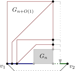
Figure 8: A recursive construction of an infinite class of 5-planar graphs requiring super-polynomial drawing area.

Theorem 6.

There exist infinitely many triconnected 5-planar graphs for which our drawing algorithm produces drawings of super-polynomial area.

Proof.

Fig.8 illustrates a recursive construction of an infinite class of 5-planar triconnected graphs with this property. The base of the construction is a “long chain” connecting $v_{1}$ and $v_{2}$ (refer to the bold drawn edges of Fig.8). Each next member, say $G_{n+O(1)}$, of this class is constructed by adding a constant number of vertices (colored black in Fig.8) to its immediate predecessor member, say $G_{n}$, of this class, as illustrated in Fig.8. If $W_{n}$ and $H_{n}$ is the width and the height of $G_{n}$, respectively, then it is not difficult to show that $W_{n+O(1)}>2W_{n}$ and $H_{n+O(1)}>2H_{n}$, which implies that the required area is asymptotically exponential. ∎

5.2 The Biconnected Case

For the 4-planar case we defined several invariants in order to keep the area of the resulting drawings polynomial. Since we drop this requirement now we can define a (simpler) new invariant for the biconnected 5-planar case. When considering a node $\mu$ in $\mathcal{T}$ and its poles $\mathcal{P}_{\mu}=\{s,t\}$, then in the drawing of $G^{\textit{pert}}_{\mu}$, $s$ and $t$ are horizontally aligned at the bottom of the drawing’s bounding box as in Fig.9a. If an $(s,t)$-edge is present, it can be drawn at the bottom. An $(s,t)$-edge only occurs in the pertinent graph of a P-node (and Q-node). Again, we use the term fixed for a pole-node that is not allowed to form a nose. We maintain the following properties through the recursive construction process: In S- and R- nodes, $s$ and $t$ are not fixed. In P- and Q-nodes, only one of them is fixed, say $s$. But similar to the 4-planar biconnected case, we may swap their roles.

(a)

(b)

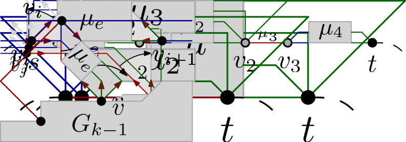
(c)

Figure 9: (a) Layout specification; $s$ and $t$ are located at the bottom. (b) P-node with an $(s,t)$-edge from a Q-node $\mu_{1}$. $s$ and $t$ form a nose in $\mu_{2},\mu_{3}$. (c) S-node example with four children $\mu_{1},\ldots,\mu_{4}$.

P-node case:

Let $\mu$ be a P-node. It is not difficult to see that $\mu$ has at most $4$ children; one of them might be a Q-node, i.e., an $(s,t)$-edge, which can be drawn at the bottom as a horizontal segment. Since P-nodes are not adjacent to each other in $\mathcal{T}$, the remaining children are S- or R-nodes. By our invariant we may form noses enabling us to stack them as in Fig.9b, as $s$ and $t$ are not fixed in them.

S-node case:

Let $\mu$ be an S-node with children $\mu_{1},\ldots,\mu_{l}$. Instead of the diagonal layout used earlier, we now align the drawings horizontally; see Fig.9c. In the S-node case, the poles inherit their pertinent degree from the children and the same holds for the property of being fixed. However, by our new invariant this is forbidden, as it clearly states that $s$ and $t$ are not fixed. It is easy to see that when $\mu_{1}$ is a P-node, $s$ is fixed by the invariant in $\mu_{1}$. In this case, we swap the roles of the poles in $\mu_{1}$ such that $s$ is not fixed. However, the other pole of $\mu_{1}$, say $v_{1}$, is fixed now. Since the skeleton of an S-node is a cycle of length at least three, $v_{1}\neq t$ holds. As a result, both $s$ and $t$ are not fixed in the resulting drawing.

R-node case:

To compute a layout of an R-node, we employ the triconnected algorithm (with $s=v_{1}$ and $t=v_{2}$). So, let $\mu$ be an R-node and $\mu_{e}$ a child of $\mu$ that corresponds to the virtual edge $e=(u,v)$ in $G^{\textit{skel}}_{\mu}$. Then, $\textit{deg}^{\textit{pert}}_{\mu_{e}}(u)\leq 3$ and $\textit{deg}^{\textit{pert}}_{\mu_{e}}(v)\leq 3$ holds. When inserting the drawing of $G^{\textit{pert}}_{\mu_{e}}$, we require at most three consecutive ports at $u$ and $v$ for the additional edges. As the triconnected algorithm assigns ports in a consecutive manner based on the relative position of the endpoints, we modify the port assignment so that an edge may have more than one port assigned. To do so, we assign each edge $e=(u,v)$ in $G^{\textit{skel}}_{\mu}$ a pair $(\textit{deg}^{\textit{pert}}_{\mu_{e}}(u),\textit{deg}^{\textit{pert}}_{\mu_{e}}(v))\in\{1,2,3\}^{2}$ that reflects the number of ports required by this edge at its endpoints. Then, we extend the triconnected algorithm such that when a port of $u$ is assigned to an edge $e=(u,v)$, $\textit{deg}^{\textit{pert}}_{\mu_{e}}(u)-1$ additional consecutive ports in clockwise or counterclockwise order are reserved. The direction depends on the different types of edges that we will discuss next.

(a)

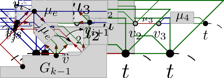
(b)

(c)

(d)

(e)

(f)

Figure 10: (a) Virtual edge $e=(v_{i},v_{i+1})$ connecting two consecutive vertices of a chain. At both endpoints the drawing of $\mu_{e}$ requires two ports. (b) Replacing $e$ in (a) with the corresponding drawing of the child $\mu_{e}$. (c) Example of an edge $e=(v_{j},v_{j}^{\prime})$ that requires three ports at $v_{j}$ and two at $v_{j}^{\prime}$. (d) Inserting the drawing of $\mu_{e}$ into (c) with $v_{j}$ being fixed and $v_{j}^{\prime}$ forming a nose. (e) Reserving ports for the nested edges. A single port for a real edge is reserved and then two ports for the virtual edge e = $(v_{i},v)$. (f) Final layout after inserting the drawing of $\mu_{e}$.

The simplest type of edges are the ones among consecutive vertices $v_{i},v_{i+1}$ of a chain. Recall that $P_{0}=\{v_{1},v_{2}\}$ is a special case and the edge $(v_{1},v_{2})$ is drawn differently. Also, the edges from $P_{0}$ to $P_{1}$ are drawn as horizontal segments; see Fig.7c. For each such edge we reserve the additional ports at $v_{i}$ in counter-clockwise order and at $v_{i+1}$ in clockwise order; see Fig.10a. So, we can later plug the drawing of the children into the layout as in Fig.10b without forming noses. The second type of edges are the ones that connect $P_{k}=\left\{v_{i},\ldots,v_{j}\right\}$ to $v_{i}^{\prime}$ and $v_{j}^{\prime}$ in $G_{k-1}$. No matter if $P_{k}$ is a singleton or a chain, we proceed by reserving the ports as in the previous case, i.e., at $v_{i}$ clockwise, ($v_{j}$ counter-clockwise, resp.) and at $v_{i}^{\prime}$ counter-clockwise ($v_{j}^{\prime}$ clockwise); see Fig.10c. In case where $(v_{i},v_{i}^{\prime})$ or $(v_{j},v_{j}^{\prime})$ is a virtual edge, we choose the poles such that $v_{i}$ ($v_{j}$ resp.) is fixed in $\mu_{(v_{i},v_{i}^{\prime})}$ ($\mu_{(v_{j},v_{j}^{\prime})}$ resp.). Thus, we can create a nose with $v_{i}^{\prime}$ ($v_{j}^{\prime}$ resp.). Having exactly the ports required at both endpoints, we insert the drawing by replacing the bend with a nose as in Fig.10d. The remaining edges from $P_{k}$ to $G_{k-1}$ in case of a singleton $P_{k}=\{v_{i}\}$ can be handled similarly; see Fig.10. Notice that during the replacement of the edges, the fixed vertex is always the upper one. The only exception are the horizontal drawn edges of a chain. There, it does not matter which one is fixed, as none of the poles has to form a nose.

Root case:

We root $\mathcal{T}$ at an arbitrarily chosen Q-node representing a real edge $(s,t)$. By our invariant we may construct a drawing with $s$ and $t$ at the bottom of the drawing’s bounding box, hence, we draw the edge $(s,t)$ below the bounding box with a ninety degree bend using the south east port at $s$ and south west port at $t$.

Theorem 7.

Given a biconnected 5-planar graph $G$, we can compute in $O(n^{2})$ time an octilinear drawing of $G$ with at most one bend per edge.

Proof.

We have shown that the ability to rotate and scale suffices to extend the result from 4-planar to 5-planar at the expense of the area. Similar to the 4-planar case, computing $\mathcal{T}$ takes linear time. Hence, the overall runtime is governed by the triconnected algorithm. ∎

5.3 The Simply Connected Case

In the following, we only outline the differences in comparison with the corresponding 4-planar case. As an invariant, the drawing of every subtree should conform to the layout depicted in Fig.11a. For a single biconnected component $b$, let $v_{c}$ refer to the cut vertex linking it to the parent. As root for the SPQR-tree $\mathcal{T}_{b}$ of $G_{b}$, we again choose a Q-node $\mu_{r}$ whose real edge is incident to $v_{c}$; see Fig.11b. Hence, the layout generated by the biconnected approach matches this scheme.

(a)

(b)

(c)

(d)

Figure 11: (a) Layout scheme for a BC-subtree rooted at $v_{c}$. (b) Rooting $\mathcal{T}_{b}$ at a Q-node $\mu_{r}$. (c) Attaching a subtree at a chain and in (d) at a singleton inside an R-node.

It remains to show that we can attach the children. Since we are able to scale and rotate, we keep things simple and look for suitable spots to attach them. Notice that in the drawings of S-nodes and chains in R-nodes all southern ports are free. Hence, we may rotate the drawings of the subtrees and attach the at most three (two for a chain) edges to $v_{c}$ there (refer to Fig.11c for an example of a chain). The only exception are the singletons. Assume that $v_{i}$ is an ordinary singleton that has one nested edge attached. Hence, it has degree four, leaving us with a single bridge to attach the component; Fig.11d. However, this does not hold in case $v_{i}=v_{n}$. Consider the case where $v_{n}$ has a nested edge and we have to attach a subtree that requires two ports. As a result $v_{n}$ has degree $3$ in $G_{b}$ and, thus, all northern ports are free.

Theorem 8.

Given a connected 5-planar graph $G$, we can compute in $O(n^{2})$ time an octilinear drawing of $G$ with at most one bend per edge.

Proof.

We described how to attach any subtree to cut vertices inside a biconnected component. Furthermore, the component itself complies with the layout scheme. In addition, this scheme enables us to compose such drawings at a cut vertex using rotations. ∎

6 A Note on Octilinear Drawings of 6-Planar Graphs

In this section, we show that it is not always possible to construct a planar octilinear drawing of a given $6$-planar graph with at most one bend per edge. In particular, we present an infinite class of 6-planar graphs, which do not admit planar octilinear drawings with at most one bend per edge.

Theorem 9.

There exists an infinite class of 6-planar graphs which do not admit planar octilinear drawings with at most one bend per edge.

Proof.

Our proof is heavily based on the following simple observation: If the outer face $\mathcal{F}(\Gamma(G))$ of a given planar octilinear drawing $\Gamma(G)$ consists of exactly three vertices, say $v,v^{\prime}$ and $v^{\prime\prime}$, that have the so-called outerdegree-property, i.e., $deg(v)=deg(v^{\prime})=6$ and $5\leq deg(v^{\prime\prime})\leq 6$, then it is not feasible to draw all edges delimiting $\mathcal{F}(\Gamma(G))$ with at most one bend per edge; one of them has to be drawn with (at least) two bends in $\Gamma(G)$. Next, we construct a specific maximal 6-planar graph, in which each face has at most one vertex of degree $5$ and at least two vertices of degree $6$; see Fig.12a. This specific graph does not admit a planar octilinear drawing with at most one bend, as its outerface is always bounded by three vertices that have the outerdegree-property.

To obtain an infinite class of 6-planar graphs with this property, we give the following recursive construction. Let $G_{1}$ and $G_{2}$ be two copies of the graph of Fig.12a. Let also $f_{i}$ be a bounded face of $G_{i}$, $i=1,2$. We proceed to subdivide each edge of $f_{i}$ by introducing a new vertex on it. We further assume that the new vertices of $f_{i}$ are pairwise adjacent (see the top part of Fig.12b). Hence, they form a triangular face, say $f_{i}^{\prime}$, in the augmented graph, say $G_{i}^{aug}$, constructed in this manner. Up to now, each of the newly introduced vertices is of degree four. Now, assume that $G_{1}^{aug}$ is drawn on the plane so that $f_{1}^{\prime}$ is a bounded face in $\Gamma(G_{1}^{aug})$, and $G_{2}^{aug}$ is drawn such that $f_{2}^{\prime}$ is the unbounded face in $\Gamma(G_{2}^{aug})$. By choosing $f_{2}^{\prime}$ as the outer face in $\Gamma(G_{2}^{aug})$ we make sure that we can connect the three degree four vertices of $f_{2}^{\prime}$ to the three degree four vertices of $f_{1}^{\prime}$ in the following way: We appropriately scale down $\Gamma(G_{2}^{aug})$ and proceed to draw it in the interior of $f_{1}^{\prime}$ without introducing any crossings (see the small gray-colored triangle of the bottom drawing of Fig.12b). If we connect the vertices of $f_{1}^{\prime}$ and $f_{2}^{\prime}$ in an “octahedron-like manner”, then all vertices of $f_{1}^{\prime}$ and $f_{2}^{\prime}$ are of degree $6$ and the resulting graph, say $G_{1}^{aug}\oplus G_{2}^{aug}$, is maximal $6$-planar and has the outerdegree-property. ∎

(a)

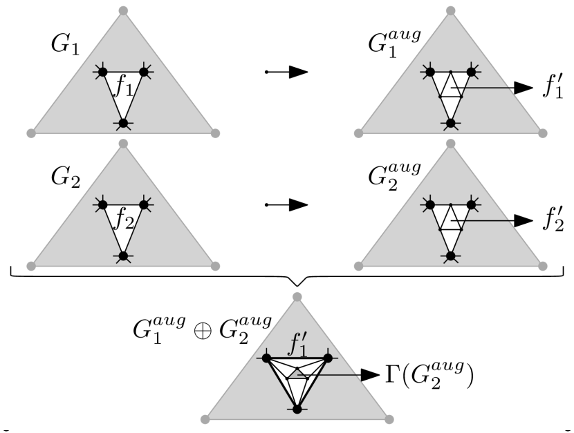
(b)

Figure 12: (a) A maximal $6$-planar graph in which each face has at most one vertex of degree $5$ (black-colored vertices) and at least two vertices of degree $6$ (gray-colored vertices). From Euler’s formula for maximal planar graphs, it follows that any graph with this property must have at least $12$ vertices of degree $5$. Hence, this is the smallest graph with this property. (b) Illustration of the recursive construction.

7 A Sample Octilinear Drawing with at most 1 bend per edge

8 Conclusions

Motivated by the fundamental role of planar octilinear drawings in map schematization, we presented algorithms for their construction with at most one bend per edge for 4- and 5-planar graphs. We also improved the known bounds on the required number of slopes for $4$- and $5$-planar drawings from $8$ and $10$, resp. ([12]) to $4$. Our work raises several open problems:

• Is it possible to construct planar octilinear drawings of 4-planar (5-planar, resp.) graphs with at most one bend per edge in $o(n^{3})$ (polynomial, resp.) area?

• Does any triangle-free 6-planar graph admit a planar octilinear drawing with at most one bend per edge?

• What is the complexity to determine whether a $6$-planar graph admits a planar octilinear drawing with at most one bend per edge?

• What is the number of necessary slopes for bendless drawings of $4$-planar graphs?

References

- [1] T. C. Biedl and G. Kant. A better heuristic for orthogonal graph drawings. In J. van Leeuwen, editor, Algorithms - ESA ’94, volume 855 of LNCS, pages 24–35. Springer Berlin Heidelberg, 1994.
- [2] T. Bläsius, M. Krug, I. Rutter, and D. Wagner. Orthogonal graph drawing with flexibility constraints. Algorithmica, 68(4):859–885, 2014.
- [3] H. L. Bodlaender and G. Tel. A note on rectilinearity and angular resolution. Journal of Graph Algorithms and Applications, 8(1):89–94, 2004.
- [4] G. Di Battista and R. Tamassia. On-line graph algorithms with SPQR-trees. In M. Paterson, editor, Automata, Languages and Programming, volume 443 of LNCS, pages 598–611. Springer Berlin Heidelberg, 1990.
- [5] E. Di Giacomo, G. Liotta, and F. Montecchiani. The planar slope number of subcubic graphs. In A. Pardo and A. Viola, editors, LATIN 2014: Theoretical Informatics, volume 8392 of LNCS, pages 132–143. Springer Berlin Heidelberg, 2014.
- [6] A. Garg and R. Tamassia. On the computational complexity of upward and rectilinear planarity testing. SIAM Journal on Computing, 31(2):601–625, 2001.
- [7] C. Gutwenger and P. Mutzel. A linear time implementation of SPQR-trees. In J. Marks, editor, Graph Drawing, volume 1984 of LNCS, pages 77–90. Springer Berlin Heidelberg, 2001.
- [8] S.-H. Hong, D. Merrick, and H. A. D. do Nascimento. Automatic visualisation of metro maps. Journal of Visual Languages and Computing, 17(3):203–224, 2006.
- [9] V. Jelínek, E. Jelínková, J. Kratochvíl, B. Lidický, M. Tesar, and T. Vyskocil. The planar slope number of planar partial 3-trees of bounded degree. Graphs and Combinatorics, 29(4):981–1005, 2013.
- [10] G. Kant. Drawing planar graphs using the lmc-ordering. In 33rd Annual Symposium on Foundations of Computer Science (FOCS ’92), pages 101–110. IEEE, 1992.
- [11] G. Kant. Hexagonal grid drawings. In E. W. Mayr, editor, Graph-Theoretic Concepts in Computer Science, volume 657 of LNCS, pages 263–276. Springer Berlin Heidelberg, 1992.
- [12] B. Keszegh, J. Pach, and D. Pálvölgyi. Drawing planar graphs of bounded degree with few slopes. SIAM Journal of Discrete Mathematics, 27(2):1171–1183, 2013.
- [13] B. Keszegh, J. Pach, D. Pálvölgyi, and G. Tóth. Drawing cubic graphs with at most five slopes. Computational Geometry, 40(2):138–147, 2008.
- [14] W. Lenhart, G. Liotta, D. Mondal, and R. I. Nishat. Planar and plane slope number of partial 2-trees. In S. Wismath and A. Wolff, editors, Graph Drawing, volume 8242 of LNCS, pages 412–423. Springer International Publishing, 2013.
- [15] P. Mukkamala and D. Pálvölgyi. Drawing cubic graphs with the four basic slopes. In M. van Kreveld and B. Speckmann, editors, Graph Drawing, volume 7034 of LNCS, pages 254–265. Springer Berlin Heidelberg, 2011.
- [16] M. Nöllenburg. Automated drawings of metro maps. Technical Report 2005-25, Fakultät für Informatik, Universität Karlsruhe, 2005.
- [17] M. Nöllenburg and A. Wolff. Drawing and labeling high-quality metro maps by mixed-integer programming. IEEE Transactions on Visualization and Computer Graphics, 17(5):626–641, 2011.
- [18] J. M. Stott, P. Rodgers, J. C. Martinez-Ovando, and S. G. Walker. Automatic metro map layout using multicriteria optimization. IEEE Transactions on Visualization and Computer Graphics, 17(1):101–114, 2011.
- [19] R. Tamassia. On embedding a graph in the grid with the minimum number of bends. SIAM Journal of Computing, 16(3):421–444, 1987.
- [20] A. Wolff. Graph drawing and cartography. In R. Tamassia, editor, Handbook of Graph Drawing and Visualization, chapter 23, pages 697–736. CRC Press, 2013.