Conformal Behavior at Four Loops and Scheme (In)Dependence

Abstract

We search for infrared zeros of the beta function and evaluate the anomalous dimension of the mass at the associated fixed point for asymptotically free vector-like fermionic gauge theories with gauge group $SU(N)$. The fixed points of the beta function are studied at the two, three and four loop level in two different explicit schemes. These are the modified regularization invariant, RI’, scheme and the minimal momentum subtraction, mMOM, scheme. The search is performed in Landau gauge where the beta function of the gauge parameter vanishes. We then compare our findings to earlier identical investigations performed in the modified minimal subtraction, $\overline{\text{MS}}$, scheme.

It is found that the value of the anomalous dimension of the mass is smaller at three and four loops than at two loops. This seems to be a generic pattern that is observed in all three different schemes. We then estimate the value of the anomalous dimension to be $\gamma\sim 0.225-0.375$ for twelve fundamental flavors and three colors, $\gamma\sim 0.500-0.593$ for two adjoint flavors and two colors and finally $\gamma\sim 1.12-1.70$ for two two-indexed flavors and three colors with the lower and upper bound set by the minimum and maximum value respectively over all three schemes and at three and four loops. Our analysis suggests that the former two theories lie in the conformal window while the latter belongs to the chirally broken phase. Preprint: CP³-Origins-2014-030 DNRF 90 & DIAS-2014-30

I Introduction

One of the key discoveries that lead to the establishment of the Standard Model of particle physics was the realization that nonabelian gauge theories under a set of appropriate conditions exhibit the phenomena of asymptotic freedom Gross:1973id ; Politzer:1973fx ; Gross:1973ju ; Gross:1974cs ; Politzer:1974fr . Physically this means that for instance in the case of the strong interactions, described by Quantum Chromo Dynamics (QCD), the quarks behave as if they are free and noninteracting at short distances.

The discovery is a consequence of a one loop computation of the beta function dictating how the coupling constant changes as one varies the energy scale. The beta function can generically be expanded as a polynomial in the coupling constant and a one loop computation reveals the first coefficient in this expansion to be negative for a sufficiently small number of matter fields. Evaluating the running of the gauge coupling as a function of the energy scale one therefore finds that in the ultraviolet the gauge coupling tends to zero canceling the mutual interaction between the matter fields prompting them to behave freely. On the other hand as the energy is decreased the value of the gauge coupling increases eventually blowing up in the deep infrared invalidating the perturbative expansion.

It should be clear that this immediately begs the question of what happens if one includes the second term in the perturbative expansion of the beta function. Is the qualitative picture of an ever increasing coupling constant at lower energies, presumably leading to confinement and chiral symmetry breaking, kept intact or could new phenomena and behavior emerge?

This question was first addressed by Caswell Caswell:1974gg and later by Banks and Zaks Banks:1981nn who computed and studied the inclusion of the second term in the beta function. Remarkably they found that as they varied the number of matter fields just below where the theory becomes asymptotically free there is a region in which the second coefficient is positive as opposed to the first coefficient which is negative. This has the dramatic effect of turning the beta function around such that it crosses zero for a finite positive value of the coupling constant instead of blowing down to minus infinity. In other words such systems must possess a nontrivial infrared fixed point. As the energy is lowered the coupling constant increases eventually settling at the fixed point value with the theory exhibiting scale invariance.

As the number of matter fields is lowered even further it was also noted that there was a critical point where the second coefficient of the beta function would eventually become negative similarly to the first coefficient. In this regime there would be no sign of scale invariance. On the contrary the phase would presumably be characterized similarly to what is expected from QCD with confinement, chiral symmetry breaking, massive composite states, etc.

Now a second question seems to be pressing us. What is the critical number of matter fields where the system transitions from a phase with scale invariance to a phase without scale invariance in the deep infrared? As we tune the number of flavors and approach, from above, the critical value where the second coefficient changes sign the fixed point value of the coupling constant blows to infinity. Again we seem to be haunted by the limits of truncating a perturbative expansion of the beta function.

In the last 30 years there has been a tremendous effort put into the task of estimating this critical value of the number of matter fields where the phase transition occurs. The phase has eventually become known as the conformal window. First, many attempts have been made to estimate the critical value of the coupling constant that is needed to trigger chiral symmetry breaking using truncated Dyson-Schwinger equations Holdom:1984sk ; Yamawaki:1985zg ; Appelquist:1986tr ; Appelquist:1986an ; Appelquist:1988yc ; Appelquist:1987fc ; Appelquist:1997dc ; Brodsky:2008be . Then by equating the critical value needed for chiral symmetry breaking with the fixed point value stemming from the two loop beta function one can obtain an estimate of the conformal window Sannino:2004qp ; Dietrich:2006cm . This approach is known as the Ladder approximation.

A different strategy has been to simulate various theories on a computer and study whether they exhibited scale invariance or not in the deep infrared. In recent years these lattice simulations have received much interests. Investigations have been concerned with a plethora of different $SU(N)$ gauge theories including systems with fundamental matter for two colors Bursa:2010xr ; Bursa:2010xn ; Karavirta:2011zg ; Appelquist:2013pqa ; Hietanen:2013fya ; Hietanen:2014xca and three colors Appelquist:2007hu ; Deuzeman:2008sc ; Deuzeman:2009mh ; Appelquist:2009ty ; Jin:2009mc ; Fodor:2009wk ; Fodor:2011tu ; Appelquist:2011dp ; Deuzeman:2012ee ; Jin:2012dw , systems with adjoint matter for two colors Catterall:2007yx ; Hietanen:2008mr ; Catterall:2008qk ; DelDebbio:2008zf ; DelDebbio:2009fd ; Bursa:2009we ; Hietanen:2009az ; DelDebbio:2010hx ; DelDebbio:2010hu ; Catterall:2011zf ; Bursa:2011ru ; DeGrand:2011qd ; Karavirta:2011mv , systems with two-indexed symmetric matter for three colors DeGrand:2008kx ; Shamir:2008pb ; Fodor:2009ar ; Shamir:2010cq ; DeGrand:2010na ; Fodor:2012ty ; DeGrand:2012yq ; DeGrand:2013uha and four colors DeGrand:2012qa and finally $SO(4)$ gauge theories with fundamental matter Hietanen:2012sz ; Hietanen:2012qd .

In this paper we attempt to estimate the boundary of the conformal window using higher order calculations of the beta function and anomalous dimension of the mass. We perform the analysis in two different explicit schemes. This is the modified regularization invariant, RI’, scheme Martinelli:1994ty ; Gracey:2003yr and the minimal momentum subtraction scheme mMOM vonSmekal:2009ae ; Celmaster:1979km ; Chetyrkin:2000fd ; Gracey:2011pf ; Gracey:2011vw ; Gracey:2013sca . We then compare our results to earlier similar investigations Ryttov:2010iz ; Pica:2010xq performed in the usual modified minimal subtraction, $\overline{\text{MS}}$, scheme. The analysis is done at the four loop level and therefore extends earlier investigations done at the three loop level Ryttov:2013hka ; Ryttov:2013ura . It is the most up-to-date and complete investigation of higher order calculations and their effect on the phase diagram for vectorial fermionic gauge theories. As we shall there is a generic pattern in our computations showing that the anomalous dimension of the mass is smaller at the three and four loop level than the corresponding evaluation at two loops.

It should be noted that all three schemes are of course related perturbatively in the sense that they give the same predictions at the ultraviolet fixed point. However as has been stressed in Ryttov:2012ur ; Ryttov:2012nt one can imagine schemes that share this property, i.e. are perturbatively related, but are not suitable for the study of infrared fixed points. For a scheme transformation to be physically acceptable it must satisfy the following conditions Ryttov:2012ur ; Ryttov:2012nt : 1) it must map a real positive value of the coupling constant $\alpha$ to a real and positive value of the coupling constant $\alpha^{\prime}$, 2) it must map a moderate value of $\alpha$ to a moderate value of $\alpha^{\prime}$, 3) the Jacobian of the scheme transformation should not vanish in the region of $\alpha$ and $\alpha^{\prime}$ of interest and 4) it must preserve the existence of the infrared zeroes of the beta functions. A priory it is not clear whether the scheme transformations connecting the $\overline{\text{MS}}$, RI’ and mMOM schemes possess these properties. In general the conversion functions are highly complicated expressions that depend on the theory under investigation, the gauge parameter, etc, and it is not clear whether they satisfy the above constraints. This provides another reason for our studies.

For completeness and the readers convenience we note that there has also been other orthogonal methods developed in order to calculate the conformal window Ryttov:2007cx ; Pica:2010mt ; Antipin:2009wr ; Appelquist:1999hr ; Appelquist:1999vs . Also studies of systems with multiple distinct fermion representations Ryttov:2009yw ; Ryttov:2010hs , Yukawa theories Molgaard:2014mqa ; Molgaard:2014hpa ; Antipin:2013sga and fermions belonging to a spinorial representation or a representation of an exceptional gauge group has been done Mojaza:2012zd . Much work trying to clarify the issues concerning scheme dependence can be found in Shrock:2013uaa ; Shrock:2014qea while additional complimentary investigations into higher order corrections can be found in Ryttov:2012qu ; Shrock:2013ca ; Shrock:2013pya ; Shrock:2013cca ; Shrock:2014zca .

The paper is organized as follows. In Section II we introduce our calculational setup while Section III is devoted to a complete presentation of our numerical results. We finally conclude in Section IV. Appendix A and B contain all useful relations and quantities used throughout the paper while all of our numerical results and associated plots can be found in Appendix C and D.

II Generalitites

Our considerations are centered on massless vector-like gauge theories with a set of $N_{f}$ Dirac fermions transforming according to a representation $r$ of the $G=SU(N)$ gauge group. At the classical level these theories enjoy scale invariance which is spoiled, however, at the quantum level. The quantum fluctuations give rise to a coupling constant which changes (or runs) as one changes the scale.

Massless vector-like fermionic gauge theories contain two dimensionless parameters. This is the gauge coupling $\alpha$ and the covariant gauge parameter $\xi$. Both of these parameters will receive quantum corrections and scale with the energy. They each have their own associated beta function $\beta_{\alpha}$ and $\beta_{\xi}$ respectively. On the most general grounds one would expect them to be coupled such that each beta function depends on both the gauge coupling and the gauge parameter. Hence we should formally write the renormalization group functions as

$$\mu\frac{d\alpha}{d\mu} = \beta_{\alpha}\left(\alpha,\xi\right)$$ (1)

$$\mu\frac{d\xi}{d\mu} = \beta_{\xi}\left(\alpha,\xi\right)$$ (2)

where $\mu$ is the scale. If we want to know the running of the coupling constant we should solve the coupled set of differential equations. In perturbation theory the beta function is an expansion in the coupling constant where in principle we can calculate order by order each term. It is important to remember that the beta function is also a scheme dependent object. By far the most popular scheme in which to calculate the beta function has been the original minimal subtraction, MS, scheme 'tHooft:1973mm or the modified minimal subtraction, $\overline{\text{MS}}$ scheme Bardeen:1978yd . Within these two schemes one enjoys the simplicity that the gauge coupling beta function becomes a function of only the coupling constant. The above two renormalization group equations decouple. Within the class of MS-type schemes Mojaza:2012mf ; Brodsky:2013vpa it can be shown that the first two coefficients of the beta function are scheme independent. This however is not true on the most general grounds where the gauge coupling beta function also depends on the gauge parameter. Here it is only the first coefficient which is scheme independent. As we will see below this is the case for the mMOM scheme but not the RI’ scheme for which the beta function of the gauge coupling actually coincides with the one in the $\overline{\text{MS}}$ scheme.

If we want to study the fixed points of the theory we need to solve the coupled set of equations

$$0 = \beta_{\alpha}\left(\alpha_{0},\xi_{0}\right)$$ (3)

$$0 = \beta_{\xi}\left(\alpha_{0},\xi_{0}\right)$$ (4)

for the fixed points values $\alpha_{0}$ and $\xi_{0}$ of the coupling constant and the gauge parameter. In addition we should classify all the fixed points. At a given loop order there will typically be many solutions to the fixed point equations for which we are only interested in the solutions that are infrared stable with $\alpha_{0}>0$. At the three loop level all the fixed points were classified in the RI’ and mMOM scheme in Ryttov:2013hka ; Ryttov:2013ura . Here we want to extend the analysis to the four loop order.

First note that $\beta_{\xi}$ is proportional to $\xi$. This is so since $\beta_{\xi}=\xi\gamma_{\xi}$ where $\gamma_{\xi}$ is the anomalous dimension of the gauge parameter. Hence we are always guaranteed to find a fixed point solution at $\xi_{0}=0$ (Landau gauge). In addition if we fix the gauge to the Landau gauge $\xi=0$ in the ultraviolet then as we evolve the renormalization group equation for the gauge parameter it is kept in the Landau gauge $\xi(\mu)=0$ for all energy scales $\mu$. It is then a matter of solving the last fixed point equation $\beta_{\alpha}\left(\alpha_{0},0\right)=0$ in order to find the first nontrivial positive solution $\alpha_{0}$. If the theory is asymptotically free this solution is then guaranteed to be infrared stable in the $\alpha$ direction. At last we remind the reader that the first coefficient of the beta function of the coupling constant is scheme independent in any scheme such that asymptotic freedom is a well defined property.

One should note that typically there will be fixed points for which $\xi_{0}\neq 0$ which are also infrared stable. At two and three loops these solutions are either found to reside in smaller ranges of the number of flavors or they fail to predict the correct limit for the anomalous dimension as one approaches the critical number of flavors where asymptotic freedom is lost Ryttov:2013hka ; Ryttov:2013ura . First in the RI’ scheme there are four independent real solutions. One solution is the Landau gauge solution, two solutions only exists for a limited number flavors and one solution does not predict the correct limit for the anomalous dimension. Second in the mMOM scheme there exists two independent real solutions. The first is again the Landau gauge solution while the second generally only exists for a limited number of flavors. In the special case of adjoint fermions the solution exists only at three loops and not at two loops.

With these considerations in mind we focus our attention at four lops on the Landau gauge solution. Although it would be desirable to do a search for all fixed points at four loops it seems reasonable in the light of the discussion presented above to initially limit ourselves to $\xi_{0}=0$. At two and three loops in both the RI’ and mMOM schemes this gives the only fully consistent and trustable solution.

As has been noted several times the beta function is a scheme dependent quantity and so is the fixed point value $\alpha_{0}$. Since one of our aims is to compare the predictions of different schemes to a given loop order we need to find a quantity which is scheme independent at the fixed point. This is the anomalous dimension of the mass $\gamma\left(\alpha,\xi\right)$. It has been computed to four loop order in both the RI’ scheme Gracey:2003yr and the mMOM scheme Gracey:2013sca in any gauge covariant gauge. This allows for a comparison with a similar analysis at four loops Ryttov:2010iz ; Pica:2010xq in the $\overline{\text{MS}}$ scheme vanRitbergen:1997va ; Vermaseren:1997fq .

Our setup should now be clear. In the Landau gauge we look for positive solutions to the fixed point equation $\beta_{\alpha}(\alpha_{0},0)=0$ and evaluate the associated anomalous dimension of the mass $\gamma(\alpha_{0},0)$. From now on we will no longer explicitly write that we are considering Landau gauge $\xi=0$.

III Discussion of Results

One can expand both the beta function and the anomalous dimension of the mass in the coupling constant

$$\beta_{\alpha}\left(\alpha\right) = -b_{1}\left(\frac{\alpha}{4\pi}\right)^{2}-b_{2}\left(\frac{\alpha}{4\pi}\right)^{3}-b_{3}\left(\frac{\alpha}{4\pi}\right)^{4}-b_{4}\left(\frac{\alpha}{4\pi}\right)^{5}+O\left(\alpha^{6}\right)$$ (5)

$$\gamma\left(\alpha\right) = c_{1}\left(\frac{\alpha}{4\pi}\right)+c_{2}\left(\frac{\alpha}{4\pi}\right)^{2}+c_{3}\left(\frac{\alpha}{4\pi}\right)^{3}+c_{4}\left(\frac{\alpha}{4\pi}\right)^{4}+O\left(\alpha^{5}\right)$$ (6)

The coefficients $b_{i}$ and $c_{i}$, $i=1\ldots 4$, have all been computed through four loop order in the $\overline{\text{MS}}$ vanRitbergen:1997va ; Vermaseren:1997fq , RI’ Gracey:2003yr and mMOM Gracey:2013sca schemes. They can be found in Appendix A. They depend on the number of colors and flavors as well as certain group invariants. We denote by $T(r)$ and $C_{2}(r)$ the trace normalization factor and quadratic Casimir respectively. These group invariants enter at every loop order At the four loop order yet another set of invariants appear in the coefficients. These are the completely symmetric fourth order tensors $d^{abcd}_{r}$. For the readers convenience we provide in Appendix B the explicit expression for all of the group invariants for all the representations used in this work. This includes the fundamental representation denoted by F, the adjoint representation denoted by G, the two-indexed symmetric representation denoted by 2S and the two-indexed antisymmetric representation denoted by 2A. The dimension of each representation is finally denoted by $d(r)$. At last we note that the coefficients also contain $\zeta_{n}\equiv\zeta(n)$ which is the Riemann zeta function.

We are searching for infrared fixed points in a range of flavors just below where asymptotic freedom is lost

$$N_{f} \leq \frac{11}{4}\frac{C_{2}(G)}{T(r)}$$ (7)

This occurs when the first coefficient of the beta function changes sign. At any loop order the beta function always has a double zero at the origin. This is the ultraviolet fixed point. In addition at two loops there is a single nontrivial zero, at three loops there is a pair of zeros which are the complex conjugate of each other and at four loops there are three nontrivial zeros. In all situations we shall pick the first positive zero away from the origin.

At four loops there is the possibility that the first positive zero away from the origin is not the only infrared stable fixed point. If there exists three distinct real zeros then if the additional two zeros are also positive then the third one away from the origin will be infrared stable while if the additional two zeros are both negative then the second negative zero away from the origin will be infrared stable. The first hypothetical situation with three positive zeros is not observed in any of the three schemes for any of the theories studied here. This fact was first observed in the $\overline{\text{MS}}$ scheme in Pica:2010xq but is now seen to occur in both the RI’ and mMOM schemes as well. The second situation is observed for certain theories but since the fixed point is at a negative value of the coupling constant these theories must be nonunitary and hence are not included. We conclude that in all three different schemes at four loops and in Landau gauge (where needed) there is only a single physical infrared fixed point.

There is also a lower bound on the number of flavors that we consider. This is fixed by the value of the coupling constant reaching order one.

In Appendix C we provide a comprehensive list of tables all with explicit values of the coupling constant and the anomalous dimension of the mass evaluated at the infrared fixed point in all three different schemes. This is done for the fundamental, adjoint and two-indexed representations and for a range of number of colors and flavors.

As one decreases the number of flavors below where asymptotic freedom is lost the value of the coupling constant at the infrared fixed point increases. We stop our search for infrared fixed points once the coupling constant reaches a value of order one. We have chosen an exception to this restriction for fermions in the fundamental and two-indexed antisymmetric representations where we have included numerical values of the coupling constant for a certain number of flavors even though $\alpha_{0}>1$. This is because $\alpha_{0}$ might be larger than one in certain schemes and at certain loop orders and less than one in other schemes and loop orders. An example of this is the theory with two colors and seven fundamental flavors where the two, three and four loop evaluations in both the $\overline{\text{MS}}$ and RI’ schemes and the two loop evaluation in the mMOM scheme predict a value $\alpha_{0}>1$ while the three and four loop evaluations in the mMOM scheme scheme predict $\alpha_{0}<1$. In such a case we have included the results in the table and indicated with parenthesis that the evaluation is not trustable since $\alpha_{0}>1$. In addition if the value of the coupling constant is larger than one then the associated value of the anomalous dimension is equally put in parenthesis to indicate that the computation is no longer trustable.

In addition in Appendix D we provide plots of the anomalous dimension as a function of the number of flavors. Each plot shows the two, three and four loop evaluation in a given scheme for different representations and various number of colors.

In order for a conformal theory not to contain negative normed states the full dimension of any spinless operator must be larger than unity Mack:1975je ; Flato:1983te ; Dobrev:1985qv . In particular it must true for the bilinear $\bar{\psi}\psi$ operator where $\psi$ is the fermion. Therefore since $D(\bar{\psi}\psi)=3-\gamma$ the anomalous dimension must be bounded by $\gamma\leq 2$ in a conformal theory. The plots in Appendix D are therefore cut off at this maximal possible value of the anomalous dimension. We stress that the conformal window not necessarily extends all the way to $\gamma=2$. For instance in the Ladder approximation the lower boundary of the conformal window is set by the anomalous dimension reaching the value unity Holdom:1984sk ; Yamawaki:1985zg ; Appelquist:1986tr ; Appelquist:1986an ; Appelquist:1988yc ; Appelquist:1987fc ; Appelquist:1997dc . Similarly in supersymmetric QCD the conformal window extends to the point where the anomalous dimension of $\tilde{\Phi}\Phi$ where $\tilde{\Phi}$ and $\Phi$ are chiral superfields reaches unity Seiberg:1994pq ; Ryttov:2007sr . However by cutting off the plots at $\gamma=2$ we allow for the largest possible value that the anomalous dimension can conceivably take at an infrared fixed point. The plots are also cut off at a number of flavors around the point at which the value of the coupling constant reaches order unity. The solid parts of the curves then correspond to $\alpha_{0}<1$ while the dashed parts correspond to $\alpha_{0}>1$.

By examining the different tables and plots the trend should be clear. Both the three and four loop evaluations of the anomalous dimension of the mass is smaller relative to the two loop evaluation. In addition in all but a few special cases the four loop result is lower than the three loop result. In the mMOM scheme for two, three and four colors with fermions in the fundamental representation and for four colors with fermions in the two-indexed antisymmetric representation the four loop evaluation is a bit larger than the three loop evaluation. The trend is seen for all representations, various numbers of colors and in all three different schemes.

It is important to ask about the reliability of the perturbative calculation. Naively one might expect that as long as $\alpha_{0}<1$ then the results can be trusted. This is not always the case however. For fermions in the adjoint and two-indexed symmetric representations the three and four loop evaluation of $\gamma$ in all three schemes are very similar. The same is true for fermions in the fundamental and two-indexed antisymmetric representation in the mMOM scheme. But for fermions in the fundamental representation and the two-indexed antisymmetric representation in the $\overline{\text{MS}}$ and RI’ schemes and for a sufficiently small number of flavors, i.e. at the lower end of the conformal window, the behavior of the anomalous dimension differs significantly between the three and four loop evaluation. This occurs even though $\alpha_{0}<1$ and perturbation theory is expected to be a reasonable approximation. This could be due to the fact that the perturbative expansion has not yet converged.

There are a few theories which are of specific interest to both the lattice and beyond the Standard Model physics communities. First is the theory with twelve fundamental flavors and three colors. Here the three and four loop evaluations of the fixed point coupling constant and anomalous dimension is in quite good agreement among all three schemes with a prediction of $\alpha_{0}\sim 0.364-0.470$ and $\gamma\sim 0.225-0.375$. Second is the theory with two adjoint flavors and two colors for which the three and four loop evaluations are almost identical. This is again the case in all three different schemes with a prediction $\alpha_{0}\sim 0.398-0.459$ and $\gamma\sim 0.500-0.593$. Third is the theory with two two-indexed symmetric flavors and three colors. At the three and four loop level the prediction of the fixed point value is $\alpha_{0}\sim 0.394-0.500$ while the anomalous dimension is $\gamma\sim 1.12-1.70$. In this case there is considerable deviation in the value of the anomalous dimension between the various loop orders and schemes.

This could be a sign of the limitations of the perturbative analysis (poor convergence of the perturbative expansion) and/or be due to the fact that the theory is not within the conformal window. Remember that the anomalous dimension is only a scheme independent quantity at a fixed point. Hence if the theory has not reached the fixed point (and never will) it is no surprise that if one attempts to compute the anomalous dimension in different schemes one will obtain a wide range of different values. The hint that this might have occurred comes from the fact that the anomalous dimension has exceeded unity and according to the Ladder approximation instead must have entered a chirally broken phase. However we warn the reader that in order to fully access whether the theory is inside or outside the conformal window requires complete nonperturbative knowledge about its dynamics.

It should also be noted that the former two theories with twelve fundamental flavors and three colors or two adjoint flavors and two colors lie very close to the point where deviations between the three and four loop evaluations in certain schemes start to become significant. Similarly this could be a sign that these theories lie very close to (but within) the boundary of the conformal window.

IV Conclusion

We have searched for infrared fixed points in theories with massless vector-like fermionic matter and gauge group $SU(N)$. This was done by analyzing the beta function of the coupling constant and the anomalous dimension of the mass at two, three and four loop level. The search was done in the RI’ and mMOM schemes and then compared to earlier studies in the $\overline{\text{MS}}$ scheme. In cases where the beta function depended on the gauge parameter the investigations were performed in the Landau gauge.

We found a generic pattern with the value of the anomalous dimension at three and four loops being smaller as compared to its two loop evaluation. This was found in all three different schemes. We then discussed specifically the prediction of the anomalous dimension for three different theories. This was twelve fundamental flavors and three colors, two adjoint flavors and two colors and two two-indexed symmetric flavors and three colors. In the first two models our prediction of the anomalous dimension was $\gamma\sim 0.225-0.375$ and $\gamma\sim 0.500-0.593$ respectively while in the third model it was $\gamma\sim 1.12-1.70$. This seems to indicate that the first two theories belong to the conformal window while the third belongs to the chirally broken phase.

Appendix A Beta Function and Anomalous Dimension of the Mass to Four Loops

A.1 $\overline{\text{MS}}$ Scheme

Coefficients in the modified minimal subtraction, $\overline{\text{MS}}$, scheme of the beta function and the anomalous dimension of the mass to four loop order

$$b_{1} = \frac{11}{3}C_{2}(G)-\frac{4}{3}T(r)N_{f}$$ (8)

$$b_{2} = \frac{34}{3}C_{2}(G)^{2}-4C_{2}(r)T(r)N_{f}-\frac{20}{3}C_{2}(G)T(r)N_{f}$$ (9)

$$b_{3} = \frac{2857}{54}C_{2}(G)^{3}+2C_{2}(r)^{2}T(r)N_{f}-\frac{205}{9}C_{2}(r)C_{2}(G)T(r)N_{f}-\frac{1415}{27}C_{2}(G)^{2}T(r)N_{f}$$ (10)

$$+\frac{44}{9}C_{2}(r)T(r)^{2}N_{f}^{2}+\frac{158}{27}C_{2}(G)T(r)^{2}N_{f}^{2}$$

$$b_{4} = \left(\frac{150653}{486}-\frac{44}{9}\zeta_{3}\right)C_{2}(G)^{4}+\left(-\frac{39143}{81}+\frac{136}{3}\zeta_{3}\right)C_{2}(G)^{3}T(r)N_{f}$$ (11)

$$+\left(\frac{7073}{243}-\frac{656}{9}\zeta_{3}\right)C_{2}(G)^{2}C_{2}(r)T(r)N_{f}+\left(-\frac{4204}{27}+\frac{352}{9}\zeta_{3}\right)C_{2}(G)C_{2}(r)^{2}T(r)N_{f}$$

$$+46C_{2}(r)^{3}T(r)N_{f}+\left(\frac{7930}{81}+\frac{224}{9}\zeta_{3}\right)C_{2}(G)^{2}T(r)^{2}N_{f}^{2}+\left(\frac{1352}{27}-\frac{704}{9}\zeta_{3}\right)C_{2}(r)^{2}T(r)^{2}N_{f}^{2}$$

$$+\left(\frac{17152}{243}+\frac{448}{9}\zeta_{3}\right)C_{2}(G)C_{2}(r)T(r)^{2}N_{f}^{2}+\frac{424}{243}C_{2}(G)T(r)^{3}N_{f}^{3}+\frac{1232}{243}C_{2}(r)T(r)^{3}N_{f}^{3}$$

$$+\left(-\frac{80}{9}+\frac{704}{3}\zeta_{3}\right)\frac{d_{G}^{abcd}d_{G}^{abcd}}{d(G)}+\left(\frac{512}{9}-\frac{1664}{3}\zeta_{3}\right)N_{f}\frac{d_{r}^{abcd}d_{G}^{abcd}}{d(G)}$$

$$+\left(-\frac{704}{9}+\frac{512}{3}\zeta_{3}\right)N_{f}^{2}\frac{d_{r}^{abcd}d_{r}^{abcd}}{d(G)}$$

$$c_{1} = 6C_{2}(r)$$ (12)

$$c_{2} = 3C_{2}(r)^{2}+\frac{97}{3}C_{2}(G)C_{2}(r)-\frac{20}{3}C_{2}(r)T(r)N_{f}$$ (13)

$$c_{3} = 129C_{2}(r)^{3}-\frac{129}{2}C_{2}(G)C_{2}(r)^{2}+\frac{11413}{54}C_{2}(G)^{2}C_{2}(r)+\left(-92+96\zeta_{3}\right)C_{2}(r)^{2}T(r)N_{f}$$ (14)

$$-\left(\frac{1112}{27}+96\zeta_{3}\right)C_{2}(G)C_{2}(r)T(r)N_{f}-\frac{280}{27}C_{2}(r)T(r)^{2}N_{f}^{2}$$

$$c_{4} = -\left(\frac{1261}{4}+672\zeta_{3}\right)C_{2}(r)^{4}+\left(\frac{15349}{6}+632\zeta_{3}\right)C_{2}(G)C_{2}(r)^{3}$$ (15)

$$+\left(-\frac{34045}{18}-304\zeta_{3}+880\zeta_{5}\right)C_{2}(G)^{2}C_{2}(r)^{2}+\left(\frac{70055}{36}+\frac{2836}{9}\zeta_{3}-880\zeta_{5}\right)C_{2}(G)^{3}C_{2}(r)$$

$$+\left(-\frac{560}{3}+1104\zeta_{3}-960\zeta_{5}\right)C_{2}(r)^{3}T(r)N_{f}+\left(-\frac{17638}{27}+736\zeta_{3}-528\zeta_{4}+160\zeta_{5}\right)C_{2}(G)C_{2}(r)^{2}T(r)N_{f}$$

$$+\left(-\frac{65459}{81}-\frac{5368}{3}\zeta_{3}+528\zeta_{4}+800\zeta_{5}\right)C_{2}(G)^{2}C_{2}(r)T(r)N_{f}$$

$$+\left(\frac{608}{27}-320\zeta_{3}+192\zeta_{4}\right)C_{2}(r)^{2}T(r)^{2}N_{f}^{2}+\left(\frac{2684}{81}+320\zeta_{3}-192\zeta_{4}\right)C_{2}(G)C_{2}(r)T(r)^{2}N_{f}^{2}$$

$$+\left(-\frac{1328}{81}+\frac{256}{9}\zeta_{3}\right)C_{2}(r)T(r)^{3}N_{f}^{3}+\left(-64+480\zeta_{3}\right)\frac{d_{r}^{abcd}d_{G}^{abcd}}{d(r)}+\left(128-960\zeta_{3}\right)N_{f}\frac{d_{r}^{abcd}d_{r}^{abcd}}{d(r)}$$

A.2 RI’ Scheme

Coefficients in the modified regularization invariant, RI’, scheme of the beta function and the anomalous dimension of the mass to four loop order and in Landau gauge $\xi=0$

$$b_{1} = \frac{11}{3}C_{2}(G)-\frac{4}{3}T(r)N_{f}$$ (16)

$$b_{2} = \frac{34}{3}C_{2}(G)^{2}-4C_{2}(r)T(r)N_{f}-\frac{20}{3}C_{2}(G)T(r)N_{f}$$ (17)

$$b_{3} = \frac{2857}{54}C_{2}(G)^{3}+2C_{2}(r)^{2}T(r)N_{f}-\frac{205}{9}C_{2}(r)C_{2}(G)T(r)N_{f}-\frac{1415}{27}C_{2}(G)^{2}T(r)N_{f}$$ (18)

$$+\frac{44}{9}C_{2}(r)T(r)^{2}N_{f}^{2}+\frac{158}{27}C_{2}(G)T(r)^{2}N_{f}^{2}$$

$$b_{4} = C_{2}(G)^{4}\left(\frac{150653}{486}-\frac{44}{9}\zeta_{3}\right)+C_{2}(G)^{3}T(r)N_{f}\left(-\frac{39143}{81}+\frac{136}{3}\zeta_{3}\right)$$ (19)

$$+C_{2}(G)^{2}C_{2}(r)T(r)N_{f}\left(\frac{7073}{243}-\frac{656}{9}\zeta_{3}\right)+C_{2}(G)C_{2}(r)^{2}T(r)N_{f}\left(-\frac{4204}{27}+\frac{352}{9}\zeta_{3}\right)$$

$$+46C_{2}(r)^{3}T(r)N_{f}+C_{2}(G)^{2}T(r)^{2}N_{f}^{2}\left(\frac{7930}{81}+\frac{224}{9}\zeta_{3}\right)+C_{2}(r)^{2}T(r)^{2}N_{f}^{2}\left(\frac{1352}{27}-\frac{704}{9}\zeta_{3}\right)$$

$$+C_{2}(G)C_{2}(r)T(r)^{2}N_{f}^{2}\left(\frac{17152}{243}+\frac{448}{9}\zeta_{3}\right)+\frac{424}{243}C_{2}(G)T(r)^{3}N_{f}^{3}+\frac{1232}{243}C_{2}(r)T(r)^{3}N_{f}^{3}$$

$$+\frac{d_{G}^{abcd}d_{G}^{abcd}}{d(G)}\left(-\frac{80}{9}+\frac{704}{3}\zeta_{3}\right)+N_{f}\frac{d_{r}^{abcd}d_{G}^{abcd}}{d(G)}\left(\frac{512}{9}-\frac{1664}{3}\zeta_{3}\right)$$

$$+N_{f}^{2}\frac{d_{r}^{abcd}d_{r}^{abcd}}{d(G)}\left(-\frac{704}{9}+\frac{512}{3}\zeta_{3}\right)$$

$$c_{1} = 6C_{2}(r)$$ (20)

$$c_{2} = \frac{1}{3}\left[185C_{2}(G)+9C_{2}(r)-52T(r)N_{f}\right]C_{2}(r)$$ (21)

$$c_{3} = \frac{1}{108}\left[\left(1944+19008\zeta_{3}\right)C_{2}(G)C_{2}(r)+\left(117428-28512\zeta_{3}\right)C_{2}(G)^{2}\right.$$ (22)

$$\left.-62960C_{2}(G)T(r)N_{f}+13932C_{2}(r)^{2}-\left(16632-3456\zeta_{3}\right)C_{2}(r)T(r)N_{f}+6848T(r)^{2}N_{f}^{2}\right]C_{2}(r)$$

$$c_{4} = -\frac{1}{3888}\left[\left(-92569118+39004740\zeta_{3}-1710720\zeta_{5}\right)C_{2}(G)^{3}C_{2}(r)\right.$$

$$+\left(10355148-22203072\zeta_{3}-1710720\zeta_{5}\right)C_{2}(G)^{2}C_{2}(r)^{2}$$

$$+\left(73217928-14239152\zeta_{3}-1244160\zeta_{5}\right)C_{2}(G)^{2}C_{2}(r)T(r)N_{f}$$

$$+\left(-33960384-1601856\zeta_{3}+10264320\zeta_{5}\right)C_{2}(G)C_{2}(r)^{3}$$

$$+\left(20983248+1347840\zeta_{3}-1244160\zeta_{5}\right)C_{2}(G)C_{2}(r)^{2}T(r)N_{f}$$

$$+\left(-16599552+580608\zeta_{3}\right)C_{2}(G)C_{2}(r)T(r)^{2}N_{f}^{2}+\left(9745920-3856896\zeta_{3}\right)C_{2}(r)^{3}T(r)N_{f}$$

$$+\left(-6653952+2571264\zeta_{3}\right)C_{2}(r)^{2}T(r)^{2}N_{f}^{2}+\left(1225692+2612736\zeta_{3}\right)C_{2}(r)^{4}$$

$$\left.+1025536C_{2}(r)T(r)^{3}N_{f}^{3}+\left(248832-1866240\zeta_{3}\right)\frac{d_{r}^{abcd}d_{G}^{abcd}}{d(r)}+\left(-497664+3732480\zeta_{3}\right)N_{f}\frac{d_{r}^{abcd}d_{r}^{abcd}}{d(r)}\right]$$

A.3 mMOM Scheme

Coefficients in the minimal momentum subtraction, mMOM, scheme of the beta function and the anomalous dimension of the mass to four loop order and in Landau gauge $\xi=0$

$$b_{1} = \frac{11}{3}C_{2}(G)-\frac{4}{3}T(r)N_{f}$$ (24)

$$b_{2} = \frac{34}{3}C_{2}(G)^{2}-4C_{2}(r)T(r)N_{f}-\frac{20}{3}C_{2}(G)T(r)N_{f}$$ (25)

$$b_{3} = -\frac{1}{288}\left[\left(-38620+5148\zeta_{3}\right)C_{2}(G)^{3}+\left(32144+6576\zeta_{3}\right)C_{2}(G)^{2}T(r)N_{f}\right.$$ (26)

$$+\left(20512-16896\zeta_{3}\right)C_{2}(G)C_{2}(r)T(r)N_{f}-\left(4416+3072\zeta_{3}\right)C_{2}(G)T(r)^{2}N_{f}^{2}-576C_{2}(r)^{2}$$

$$\left.+\left(-5888+6144\zeta_{3}\right)C_{2}(r)T(r)^{2}N_{f}^{2}\right]$$

$$b_{4} = -\frac{1}{10368}\left[\left(-22106704+5509416\zeta_{3}+3090780\zeta_{5}\right)C_{2}(G)^{4}\right.$$ (27)

$$+\left(23501280-1217376\zeta_{3}-5178960\zeta_{5}\right)C_{2}(G)^{3}T(r)N_{f}$$

$$+\left(17477280-7050240\zeta_{3}-6082560\zeta_{5}\right)C_{2}(G)^{2}C_{2}(r)T(r)N_{f}$$

$$+\left(-5719680-1654272\zeta_{3}+1474560\zeta_{5}\right)C_{2}(G)^{2}T(r)^{2}N_{f}^{2}$$

$$+\left(-607104-7907328\zeta_{3}+12165120\zeta_{5}\right)C_{2}(G)C_{2}(r)^{2}T(r)N_{f}$$

$$+\left(-10861056+4755456\zeta_{3}+2211840\zeta_{5}\right)C_{2}(G)C_{2}(r)T(r)^{2}N_{f}^{2}$$

$$+\left(229376+344064\zeta_{3}\right)C_{2}(G)T(r)^{3}N_{f}^{3}-476928C_{2}(r)^{3}T(r)N_{f}$$

$$+\left(267264+3538944\zeta_{3}-4423680\zeta_{5}\right)C_{2}(r)^{2}T(r)^{2}N_{f}^{2}+\left(1327104-884736\zeta_{3}\right)C_{2}(r)T(r)^{3}N_{f}^{3}$$

$$+\left(92160-2433024\zeta_{3}\right)\frac{d_{G}^{abcd}d_{G}^{abcd}}{d(G)}+\left(-589824+5750784\zeta_{3}\right)N_{f}\frac{d_{r}^{abcd}d_{G}^{abcd}}{d(G)}$$

$$\left.+\left(811008-1769472\zeta_{3}\right)N_{f}^{2}\frac{d_{r}^{abcd}d_{r}^{abcd}}{d(G)}\right]$$

$$c_{1} = 6C_{2}(r)$$ (28)

$$c_{2} = \frac{1}{2}\left[6C_{2}(r)+67C_{2}(G)-8T(r)N_{f}\right]C_{2}(r)$$ (29)

$$c_{3} = -\frac{1}{24}\left[\left(-10095+5634\zeta_{3}\right)C_{2}(G)^{2}+\left(244-4224\zeta_{3}\right)C_{2}(G)C_{2}(r)\right.$$ (30)

$$+\left(3888-1152\zeta_{3}\right)C_{2}(G)T(r)N_{f}-3096C_{2}(r)^{2}+\left(736+1536\zeta_{3}\right)C_{2}(r)T(r)N_{f}$$

$$\left.-384T(r)^{2}N_{f}^{2}\right]C_{2}(r)$$

$$c_{4} = -\frac{1}{2592}\left[\left(-10139319+16036470\zeta_{3}-6334605\zeta_{5}\right)C_{2}(G)^{3}C_{2}(r)\right.$$ (31)

$$+\left(-2188530-10029096\zeta_{3}+3421440\zeta_{5}\right)C_{2}(G)^{2}C_{2}(r)^{2}$$

$$+\left(8403640-15748128\zeta_{3}+2737152\zeta_{4}+4147200\zeta_{5}\right)C_{2}(G)^{2}C_{2}(r)T(r)N_{f}$$

$$+\left(-4669704+2208384\zeta_{3}+6842880\zeta_{5}\right)C_{2}(G)C_{2}(r)^{3}$$

$$+\left(-2214048+7091712\zeta_{3}-2737152\zeta_{4}+1244160\zeta_{5}\right)C_{2}(G)C_{2}(r)^{2}T(r)N_{f}$$

$$+\left(-2128192+2405376\zeta_{3}-995328\zeta_{4}\right)C_{2}(G)C_{2}(r)T(r)^{2}N_{f}^{2}$$

$$+\left(-817128-1741824\zeta_{3}\right)C_{2}(r)^{4}+\left(3509568+4935168\zeta_{3}-7464960\zeta_{5}\right)C_{2}(r)^{3}T(r)N_{f}$$

$$+\left(-605568-1327104\zeta_{3}+995328\zeta_{4}\right)C_{2}(r)^{2}T(r)^{2}N_{f}^{2}+\left(-2048+147456\zeta_{3}\right)C_{2}(r)T(r)^{3}N_{f}^{3}$$

$$+\left(-165888+1244160\zeta_{3}\right)\frac{d_{r}^{abcd}d_{G}^{abcd}}{d(r)}+\left(331776-2488320\zeta_{3}\right)N_{f}\frac{d_{r}^{abcd}d_{r}^{abcd}}{d(r)}$$

Appendix B Group Invariants for $SU(N)$

$r$	$d(r)$	$T(r)$	$C_{2}(r)$	$d^{abcd}_{r}d^{abcd}_{G}$	$d^{abcd}_{r}d^{abcd}_{r}$
F	$N$	$\frac{1}{2}$	$\frac{N^{2}-1}{2N}$	$\frac{N(N^{2}-1)(N^{2}+6)}{48}$	$\frac{(N^{2}-1)\left(N^{4}-6N^{2}+18\right)}{96N^{2}}$
G	$N^{2}-1$	$N$	$N$	$\frac{N^{2}\left(N^{2}-1\right)\left(N^{2}+36\right)}{24}$	$\frac{N^{2}\left(N^{2}-1\right)\left(N^{2}+36\right)}{24}$
2S	$\frac{N(N+1)}{2}$	$\frac{N+2}{2}$	$\frac{(N-1)(N+2)}{N}$	$\frac{N(N^{2}-1)(N+2)\left(N^{2}+6N+24\right)}{48}$	$\frac{(N^{2}-1)(N+2)\left(N^{5}+14N^{4}+72N^{3}-48N^{2}-288N+576\right)}{96N^{2}}$
2A	$\frac{N(N-1)}{2}$	$\frac{N-2}{2}$	$\frac{(N+1)(N-2)}{N}$	$\frac{N(N^{2}-1)(N-2)\left(N^{2}-6N+24\right)}{48}$	$\frac{(N^{2}-1)(N-2)\left(N^{5}-14N^{4}+72N^{3}+48N^{2}-288N-576\right)}{96N^{2}}$

Appendix C Values of the Coupling Constant and Anomalous Dimension of the Mass at Fixed Points

F		$\overline{\text{MS}}$			RI’			mMOM
$N$	$N_{f}$	$\alpha_{2l}$	$\alpha_{3l}$	$\alpha_{4l}$	$\alpha_{2l}$	$\alpha_{3l}$	$\alpha_{4l}$	$\alpha_{2l}$	$\alpha_{3l}$	$\alpha_{4l}$
2	6	(11.4)	(1.65)	(2.40)	(11.4)	(1.65)	(2.40)	(11.4)	(1.26)	(1.11)
2	7	(2.83)	(1.05)	(1.21)	(2.83)	(1.05)	(1.21)	(2.83)	0.854	0.790
2	8	(1.26)	0.688	0.760	(1.26)	0.688	0.760	(1.26)	0.588	0.571
2	9	0.595	0.418	0.444	0.595	0.418	0.444	0.595	0.377	0.377
2	10	0.231	0.196	0.200	0.231	0.196	0.200	0.231	0.187	0.188
3	9	(5.24)	(1.03)	(1.07)	(5.24)	(1.03)	(1.07)	(5.24)	0.810	0.690
3	10	(2.21)	0.764	0.815	(2.21)	0.764	0.815	(2.21)	0.621	0.556
3	11	(1.23)	0.579	0.626	(1.23)	0.579	0.626	(1.23)	0.485	0.453
3	12	0.754	0.435	0.470	0.754	0.435	0.470	0.754	0.377	0.364
3	13	0.468	0.317	0.337	0.468	0.317	0.337	0.468	0.283	0.281
3	14	0.278	0.215	0.224	0.278	0.215	0.224	0.278	0.198	0.199
3	15	0.143	0.123	0.126	0.143	0.123	0.126	0.143	0.118	0.119
3	16	0.0416	0.0397	0.0398	0.0416	0.0397	0.0398	0.0416	0.0392	0.0392
4	12	(3.54)	0.754	0.759	(3.54)	0.754	0.759	(3.54)	0.600	0.507
4	13	(1.85)	0.604	0.628	(1.85)	0.604	0.628	(1.85)	0.490	0.432
4	14	(1.16)	0.489	0.521	(1.16)	0.489	0.521	(1.16)	0.406	0.371
4	15	0.783	0.397	0.428	0.783	0.397	0.428	0.783	0.338	0.318
4	16	0.546	0.320	0.345	0.546	0.320	0.345	0.546	0.278	0.269
4	17	0.384	0.254	0.271	0.384	0.254	0.271	0.384	0.226	0.223
4	18	0.266	0.194	0.205	0.266	0.194	0.205	0.266	0.177	0.177
4	19	0.175	0.140	0.145	0.175	0.140	0.145	0.175	0.131	0.132
4	20	0.105	0.0907	0.0924	0.105	0.0907	0.0924	0.105	0.0868	0.0873
4	21	0.0472	0.0441	0.0444	0.0472	0.0441	0.0444	0.0472	0.0432	0.0433

Table 1: Values of the coupling constant at the infrared fixed point at two, three and four loop level in the $\overline{\text{MS}}$, RI’ and mMOM schemes. The fermions are in the fundamental representation of the $SU(N)$ gauge group.

F		$\overline{\text{MS}}$			RI’			mMOM
$N$	$N_{f}$	$\gamma_{2l}$	$\gamma_{3l}$	$\gamma_{4l}$	$\gamma_{2l}$	$\gamma_{3l}$	$\gamma_{4l}$	$\gamma_{2l}$	$\gamma_{3l}$	$\gamma_{4l}$
2	6	(33.2)	(0.925)	(-4.02)	(49.7)	(2.06)	(-0.297)	(39.6)	(1.03)	(1.39)
2	7	(2.67)	(0.457)	(0.0325)	(3.49)	(0.671)	(-0.0227)	(3.12)	0.523	0.628
2	8	(0.752)	0.272	0.204	(0.872)	0.312	0.163	(0.849)	0.300	0.338
2	9	0.275	0.161	0.157	0.293	0.166	0.152	0.299	0.169	0.179
2	10	0.0910	0.0738	0.0748	0.0924	0.0740	0.0746	0.0950	0.0748	0.0759
3	9	(19.8)	(1.06)	(-0.143)	(29.0)	(2.23)	(1.46)	(23.4)	1.19	1.41
3	10	(4.19)	0.647	0.156	(5.62)	1.04	0.342	(4.88)	0.735	0.850
3	11	(1.61)	0.439	0.250	(1.99)	0.572	0.221	(1.85)	0.492	0.558
3	12	0.773	0.312	0.253	0.888	0.354	0.225	0.866	0.340	0.375
3	13	0.404	0.220	0.210	0.439	0.232	0.120	0.443	0.233	0.249
3	14	0.212	0.146	0.147	0.221	0.149	0.145	0.227	0.151	0.157
3	15	0.0997	0.0826	0.0836	0.101	0.0828	0.0834	0.104	0.0835	0.0847
3	16	0.0272	0.0258	0.0259	0.0272	0.0258	0.0259	0.0276	0.0259	0.0259
4	12	(17.3)	1.11	0.0584	(25.2)	2.28	1.56	(20.4)	1.24	1.43
4	13	(5.38)	0.755	0.192	(7.33)	1.27	0.558	(6.28)	0.856	0.978
4	14	(2.45)	0.552	0.259	(3.13)	0.784	0.301	(2.82)	0.622	0.706
4	15	1.32	0.420	0.281	1.59	0.523	0.253	1.50	0.466	0.522
4	16	0.778	0.325	0.269	0.892	0.368	0.243	0.871	0.354	0.388
4	17	0.481	0.251	0.234	0.528	0.267	0.221	0.529	0.267	0.287
4	18	0.301	0.189	0.187	0.318	0.194	0.182	0.325	0.197	0.207
4	19	0.183	0.134	0.136	0.189	0.136	0.135	0.194	0.138	0.142
4	20	0.102	0.0854	0.0865	0.104	0.0856	0.0863	0.106	0.0864	0.0875
4	21	0.0440	0.0407	0.0409	0.0441	0.0407	0.0409	0.0449	0.0408	0.0409

Table 2: Values of the anomalous dimension of the mass at the infrared fixed point at two, three and four loop level in the $\overline{\text{MS}}$, RI’ and mMOM schemes. The fermions are in the fundamental representation of the $SU(N)$ gauge group.

G		$\overline{\text{MS}}$			RI’			mMOM
$N$	$N_{f}$	$\alpha_{2l}$	$\alpha_{3l}$	$\alpha_{4l}$	$\alpha_{2l}$	$\alpha_{3l}$	$\alpha_{4l}$	$\alpha_{2l}$	$\alpha_{3l}$	$\alpha_{4l}$
2	2	0.628	0.459	0.450	0.628	0.459	0.450	0.628	0.424	0.398
3	2	0.419	0.306	0.308	0.419	0.306	0.308	0.419	0.283	0.270
4	2	0.314	0.229	0.234	0.314	0.229	0.234	0.314	0.212	0.204

Table 3: Values of the coupling constant at the infrared fixed point at two, three and four loop level in the $\overline{\text{MS}}$, RI’ and mMOM schemes. The fermions are in the adjoint representation of the $SU(N)$ gauge group.

G		$\overline{\text{MS}}$			RI’			mMOM
$N$	$N_{f}$	$\gamma_{2l}$	$\gamma_{3l}$	$\gamma_{4l}$	$\gamma_{2l}$	$\gamma_{3l}$	$\gamma_{4l}$	$\gamma_{2l}$	$\gamma_{3l}$	$\gamma_{4l}$
2	2	0.820	0.543	0.500	0.900	0.593	0.518	0.885	0.569	0.559
3	2	0.820	0.543	0.523	0.900	0.593	0.541	0.885	0.569	0.568
4	2	0.820	0.543	0.532	0.900	0.593	0.550	0.885	0.569	0.571

Table 4: Values of the anomalous dimension of the mass at the infrared fixed point at two, three and four loop level in the $\overline{\text{MS}}$, RI’ and mMOM schemes. The fermions are in the adjoint representation of the $SU(N)$ gauge group.

2S		$\overline{\text{MS}}$			RI’			mMOM
$N$	$N_{f}$	$\alpha_{2l}$	$\alpha_{3l}$	$\alpha_{4l}$	$\alpha_{2l}$	$\alpha_{3l}$	$\alpha_{4l}$	$\alpha_{2l}$	$\alpha_{3l}$	$\alpha_{4l}$
3	2	0.842	0.500	0.470	0.842	0.500	0.470	0.842	0.460	0.394
3	3	0.0849	0.0790	0.0795	0.0849	0.0790	0.0795	0.0849	0.0771	0.0771
4	2	0.967	0.485	0.440	0.967	0.485	0.440	0.967	0.451	0.358
4	3	0.152	0.129	0.131	0.152	0.129	0.131	0.152	0.123	0.122

Table 5: Values of the coupling constant at the infrared fixed point at two, three and four loop level in the $\overline{\text{MS}}$, RI’ and mMOM schemes. The fermions are in the two-indexed symmetric representation of the $SU(N)$ gauge group.

2S		$\overline{\text{MS}}$			RI’			mMOM
$N$	$N_{f}$	$\gamma_{2l}$	$\gamma_{3l}$	$\gamma_{4l}$	$\gamma_{2l}$	$\gamma_{3l}$	$\gamma_{4l}$	$\gamma_{2l}$	$\gamma_{3l}$	$\gamma_{4l}$
3	2	2.44	1.28	1.12	2.96	1.70	1.55	2.69	1.42	1.26
3	3	0.144	0.133	0.133	0.145	0.133	0.133	0.147	0.133	0.134
4	2	4.82	2.08	1.79	6.24	3.19	3.30	5.37	2.44	1.93
4	3	0.381	0.313	0.315	0.395	0.319	0.316	0.400	0.319	0.321

Table 6: Values of the anomalous dimension of the mass at the infrared fixed point at two, three and four loop level in the $\overline{\text{MS}}$, RI’ and mMOM schemes. The fermions are in the two-indexed symmetric representation of the $SU(N)$ gauge group.

2A		$\overline{\text{MS}}$			RI’			mMOM
$N$	$N_{f}$	$\alpha_{2l}$	$\alpha_{3l}$	$\alpha_{4l}$	$\alpha_{2l}$	$\alpha_{3l}$	$\alpha_{4l}$	$\alpha_{2l}$	$\alpha_{3l}$	$\alpha_{4l}$
4	6	(2.17)	0.664	0.770	(2.17)	0.664	0.770	(2.17)	0.557	0.482
4	7	0.890	0.437	0.502	0.890	0.437	0.502	0.890	0.376	0.352
4	8	0.449	0.287	0.319	0.448	0.287	0.319	0.449	0.255	0.252
4	9	0.225	0.174	0.184	0.225	0.174	0.184	0.225	0.161	0.162
4	10	0.0904	0.0804	0.0819	0.0904	0.0804	0.0819	0.0904	0.0775	0.0781

Table 7: Values of the coupling constant at the infrared fixed point at two, three and four loop level in the $\overline{\text{MS}}$, RI’ and mMOM schemes. The fermions are in the two-indexed antisymmetric representation of the $SU(N)$ gauge group.

2A		$\overline{\text{MS}}$			RI’			mMOM
$N$	$N_{f}$	$\gamma_{2l}$	$\gamma_{3l}$	$\gamma_{4l}$	$\gamma_{2l}$	$\gamma_{3l}$	$\gamma_{4l}$	$\gamma_{2l}$	$\gamma_{3l}$	$\gamma_{4l}$
4	6	(9.78)	1.38	0.293	(13.7)	2.57	3.03	(11.3)	1.57	1.81
4	7	2.19	0.695	0.435	2.73	0.942	0.565	2.48	0.770	0.885
4	8	0.802	0.402	0.368	0.904	0.449	0.352	0.885	0.430	0.477
4	9	0.331	0.228	0.232	0.348	0.234	0.228	0.354	0.236	0.248
4	10	0.117	0.101	0.103	0.118	0.101	0.102	0.121	0.102	0.103

Table 8: Values of the anomalous dimension of the mass at the infrared fixed point at two, three and four loop level in the $\overline{\text{MS}}$, RI’ and mMOM schemes. The fermions are in the two-indexed antisymmetric representation of the $SU(N)$ gauge group.

Appendix D Comparison of the Anomalous Dimension at Different Loop Orders

Figure 1: In all the plots below blue curves correspond to two loops, red curves correspond to three loops and green curves correspond to four loops. In addition if the fixed point value $\alpha_{0}<1$ then the curve is solid while if $\alpha_{0}>1$ then the curve is dashed.

Figure 2: The anomalous dimension at an infrared fixed point as a function of the number of flavors. The fermions are in the fundamental representation, F, and the number of colors is $N=2$.

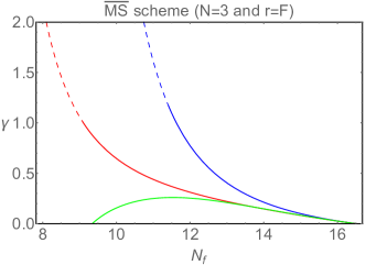
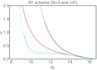
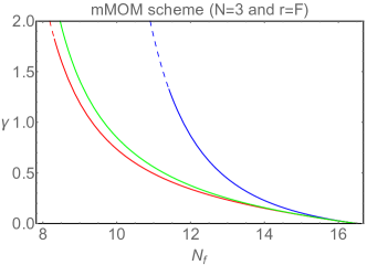
Figure 3: The anomalous dimension at an infrared fixed point as a function of the number of flavors. The fermions are in the fundamental representation, F, and the number of colors is $N=3$.

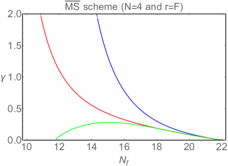
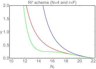
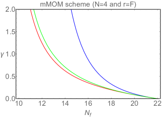
Figure 4: The anomalous dimension at an infrared fixed point as a function of the number of flavors. The fermions are in the fundamental representation, F, and the number of colors is $N=4$.

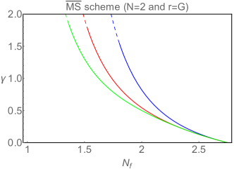
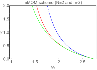
Figure 5: The anomalous dimension at an infrared fixed point as a function of the number of flavors. The fermions are in the adjoint representation, G, and the number of colors is $N=2$.

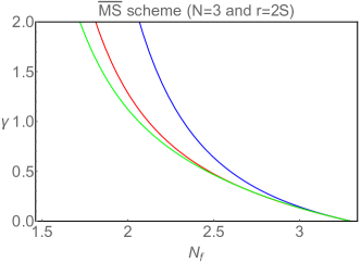
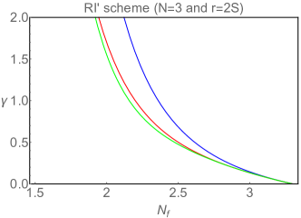
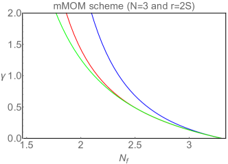
Figure 6: The anomalous dimension at an infrared fixed point as a function of the number of flavors. The fermions are in the two-indexed symmetric representation, 2S, and the number of colors is $N=3$.

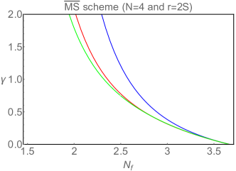
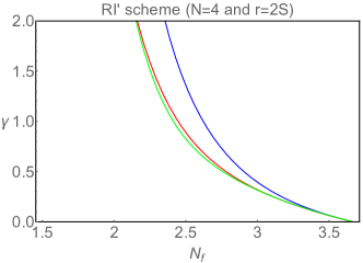
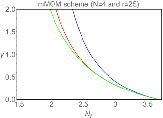
Figure 7: The anomalous dimension at an infrared fixed point as a function of the number of flavors. The fermions are in the two-indexed symmetric representation, 2S, and the number of colors is $N=4$.

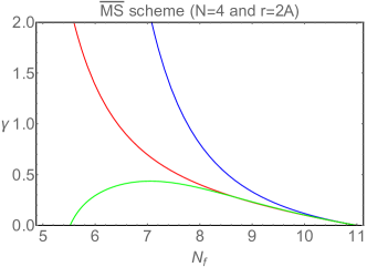
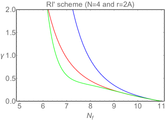
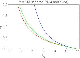
Figure 8: The anomalous dimension at an infrared fixed point as a function of the number of flavors. The fermions are in the two-indexed antisymmetric representation, 2A, and the number of colors is $N=4$.

References

- (1) D. J. Gross and F. Wilczek, “Ultraviolet Behavior of Nonabelian Gauge Theories,” Phys. Rev. Lett. 30, 1343 (1973).
- (2) H. D. Politzer, “Reliable Perturbative Results for Strong Interactions?,” Phys. Rev. Lett. 30, 1346 (1973).
- (3) D. J. Gross and F. Wilczek, “Asymptotically Free Gauge Theories. 1,” Phys. Rev. D 8, 3633 (1973).
- (4) D. J. Gross and F. Wilczek, “Asymptotically Free Gauge Theories. 2.,” Phys. Rev. D 9, 980 (1974).
- (5) H. D. Politzer, “Asymptotic Freedom: An Approach to Strong Interactions,” Phys. Rept. 14, 129 (1974).
- (6) W. E. Caswell, “Asymptotic Behavior of Nonabelian Gauge Theories to Two Loop Order,” Phys. Rev. Lett. 33, 244 (1974).
- (7) T. Banks and A. Zaks, “On the Phase Structure of Vector-Like Gauge Theories with Massless Fermions,” Nucl. Phys. B 196, 189 (1982).
- (8) B. Holdom, “Techniodor,” Phys. Lett. B 150, 301 (1985).
- (9) K. Yamawaki, M. Bando and K. -i. Matumoto, “Scale Invariant Technicolor Model and a Technidilaton,” Phys. Rev. Lett. 56, 1335 (1986).
- (10) T. Appelquist and L. C. R. Wijewardhana, “Chiral Hierarchies and Chiral Perturbations in Technicolor,” Phys. Rev. D 35, 774 (1987).
- (11) T. W. Appelquist, D. Karabali and L. C. R. Wijewardhana, “Chiral Hierarchies and the Flavor Changing Neutral Current Problem in Technicolor,” Phys. Rev. Lett. 57, 957 (1986).
- (12) T. Appelquist, K. D. Lane and U. Mahanta, “On The Ladder Approximation For Spontaneous Chiral Symmetry Breaking,” Phys. Rev. Lett. 61, 1553 (1988).
- (13) T. Appelquist and L. C. R. Wijewardhana, “Chiral Hierarchies from Slowly Running Couplings in Technicolor Theories,” Phys. Rev. D 36, 568 (1987).
- (14) T. Appelquist and S. B. Selipsky, “Instantons and the chiral phase transition,” Phys. Lett. B 400, 364 (1997) [hep-ph/9702404].
- (15) S. J. Brodsky and R. Shrock, “Maximum Wavelength of Confined Quarks and Gluons and Properties of Quantum Chromodynamics,” Phys. Lett. B 666, 95 (2008) [arXiv:0806.1535 [hep-th]].
- (16) F. Sannino and K. Tuominen, “Orientifold theory dynamics and symmetry breaking,” Phys. Rev. D 71, 051901 (2005) [hep-ph/0405209].
- (17) D. D. Dietrich and F. Sannino, “Conformal window of SU(N) gauge theories with fermions in higher dimensional representations,” Phys. Rev. D 75, 085018 (2007) [hep-ph/0611341].
- (18) F. Bursa, L. Del Debbio, L. Keegan, C. Pica and T. Pickup, “Mass anomalous dimension and running of the coupling in SU(2) with six fundamental fermions,” PoS LATTICE 2010, 070 (2010) [arXiv:1010.0901 [hep-ph]].
- (19) F. Bursa, L. Del Debbio, L. Keegan, C. Pica and T. Pickup, “Mass anomalous dimension in SU(2) with six fundamental fermions,” Phys. Lett. B 696, 374 (2011) [arXiv:1007.3067 [hep-ph]].
- (20) T. Karavirta, J. Rantaharju, K. Rummukainen and K. Tuominen, “Determining the conformal window: SU(2) gauge theory with = 4, 6 and 10 fermion flavours,” JHEP 1205, 003 (2012) [arXiv:1111.4104 [hep-lat]].
- (21) T. Appelquist, R. C. Brower, M. I. Buchoff, M. Cheng, G. T. Fleming, J. Kiskis, M. F. Lin and E. T. Neil et al., “Two-Color Theory with Novel Infrared Behavior,” Phys. Rev. Lett. 112, 111601 (2014) [arXiv:1311.4889 [hep-ph]].
- (22) A. Hietanen, R. Lewis, C. Pica and F. Sannino, “Composite Goldstone Dark Matter: Experimental Predictions from the Lattice,” arXiv:1308.4130 [hep-ph].
- (23) A. Hietanen, R. Lewis, C. Pica and F. Sannino, “Fundamental Composite Higgs Dynamics on the Lattice: SU(2) with Two Flavors,” arXiv:1404.2794 [hep-lat].
- (24) T. Appelquist, G. T. Fleming and E. T. Neil, “Lattice study of the conformal window in QCD-like theories,” Phys. Rev. Lett. 100, 171607 (2008) [Erratum-ibid. 102, 149902 (2009)] [arXiv:0712.0609 [hep-ph]].
- (25) A. Deuzeman, M. P. Lombardo and E. Pallante, “The Physics of eight flavours,” Phys. Lett. B 670, 41 (2008) [arXiv:0804.2905 [hep-lat]].
- (26) A. Deuzeman, M. P. Lombardo and E. Pallante, “Evidence for a conformal phase in SU(N) gauge theories,” Phys. Rev. D 82, 074503 (2010) [arXiv:0904.4662 [hep-ph]].
- (27) T. Appelquist, G. T. Fleming and E. T. Neil, “Lattice Study of Conformal Behavior in SU(3) Yang-Mills Theories,” Phys. Rev. D 79, 076010 (2009) [arXiv:0901.3766 [hep-ph]].
- (28) X. -Y. Jin and R. D. Mawhinney, “Lattice QCD with 8 and 12 degenerate quark flavors,” PoS LAT 2009, 049 (2009) [arXiv:0910.3216 [hep-lat]].
- (29) Z. Fodor, K. Holland, J. Kuti, D. Nogradi and C. Schroeder, “Nearly conformal gauge theories in finite volume,” Phys. Lett. B 681, 353 (2009) [arXiv:0907.4562 [hep-lat]].
- (30) Z. Fodor, K. Holland, J. Kuti, D. Nogradi, C. Schroeder, K. Holland, J. Kuti and D. Nogradi et al., “Twelve massless flavors and three colors below the conformal window,” Phys. Lett. B 703, 348 (2011) [arXiv:1104.3124 [hep-lat]].
- (31) T. Appelquist, G. T. Fleming, M. F. Lin, E. T. Neil and D. A. Schaich, “Lattice Simulations and Infrared Conformality,” Phys. Rev. D 84, 054501 (2011) [arXiv:1106.2148 [hep-lat]].
- (32) A. Deuzeman, M. P. Lombardo, T. Nunes Da Silva and E. Pallante, “The bulk transition of QCD with twelve flavors and the role of improvement,” Phys. Lett. B 720, 358 (2013) [arXiv:1209.5720 [hep-lat]].
- (33) X. -Y. Jin and R. D. Mawhinney, “Lattice QCD with 12 Degenerate Quark Flavors,” PoS LATTICE 2011, 066 (2011) [arXiv:1203.5855 [hep-lat]].
- (34) S. Catterall and F. Sannino, “Minimal walking on the lattice,” Phys. Rev. D 76, 034504 (2007) [arXiv:0705.1664 [hep-lat]].
- (35) A. J. Hietanen, J. Rantaharju, K. Rummukainen and K. Tuominen, “Spectrum of SU(2) lattice gauge theory with two adjoint Dirac flavours,” JHEP 0905, 025 (2009) [arXiv:0812.1467 [hep-lat]].
- (36) S. Catterall, J. Giedt, F. Sannino and J. Schneible, “Phase diagram of SU(2) with 2 flavors of dynamical adjoint quarks,” JHEP 0811, 009 (2008) [arXiv:0807.0792 [hep-lat]].
- (37) L. Del Debbio, A. Patella and C. Pica, “Higher representations on the lattice: Numerical simulations. SU(2) with adjoint fermions,” Phys. Rev. D 81, 094503 (2010) [arXiv:0805.2058 [hep-lat]].
- (38) L. Del Debbio, B. Lucini, A. Patella, C. Pica and A. Rago, “Conformal versus confining scenario in SU(2) with adjoint fermions,” Phys. Rev. D 80, 074507 (2009) [arXiv:0907.3896 [hep-lat]].
- (39) F. Bursa, L. Del Debbio, L. Keegan, C. Pica and T. Pickup, “Mass anomalous dimension in SU(2) with two adjoint fermions,” Phys. Rev. D 81, 014505 (2010) [arXiv:0910.4535 [hep-ph]].
- (40) A. J. Hietanen, K. Rummukainen and K. Tuominen, “Evolution of the coupling constant in SU(2) lattice gauge theory with two adjoint fermions,” Phys. Rev. D 80, 094504 (2009) [arXiv:0904.0864 [hep-lat]].
- (41) L. Del Debbio, B. Lucini, A. Patella, C. Pica and A. Rago, “The infrared dynamics of Minimal Walking Technicolor,” Phys. Rev. D 82, 014510 (2010) [arXiv:1004.3206 [hep-lat]].
- (42) L. Del Debbio, B. Lucini, A. Patella, C. Pica and A. Rago, “Mesonic spectroscopy of Minimal Walking Technicolor,” Phys. Rev. D 82, 014509 (2010) [arXiv:1004.3197 [hep-lat]].
- (43) S. Catterall, L. Del Debbio, J. Giedt and L. Keegan, “MCRG Minimal Walking Technicolor,” Phys. Rev. D 85 (2012) 094501 [arXiv:1108.3794 [hep-ph]].
- (44) F. Bursa, L. Del Debbio, D. Henty, E. Kerrane, B. Lucini, A. Patella, C. Pica and T. Pickup et al., “Improved Lattice Spectroscopy of Minimal Walking Technicolor,” Phys. Rev. D 84, 034506 (2011) [arXiv:1104.4301 [hep-lat]].
- (45) T. DeGrand, Y. Shamir and B. Svetitsky, “Infrared fixed point in SU(2) gauge theory with adjoint fermions,” Phys. Rev. D 83, 074507 (2011) [arXiv:1102.2843 [hep-lat]].
- (46) T. Karavirta, A. Mykkanen, J. Rantaharju, K. Rummukainen and K. Tuominen, “Nonperturbative improvement of SU(2) lattice gauge theory with adjoint or fundamental flavors,” JHEP 1106, 061 (2011) [arXiv:1101.0154 [hep-lat]].
- (47) T. DeGrand, Y. Shamir and B. Svetitsky, “Phase structure of SU(3) gauge theory with two flavors of symmetric-representation fermions,” Phys. Rev. D 79, 034501 (2009) [arXiv:0812.1427 [hep-lat]].
- (48) Y. Shamir, B. Svetitsky and T. DeGrand, “Zero of the discrete beta function in SU(3) lattice gauge theory with color sextet fermions,” Phys. Rev. D 78, 031502 (2008) [arXiv:0803.1707 [hep-lat]].
- (49) Z. Fodor, K. Holland, J. Kuti, D. Nogradi and C. Schroeder, “Chiral properties of SU(3) sextet fermions,” JHEP 0911, 103 (2009) [arXiv:0908.2466 [hep-lat]].
- (50) Y. Shamir, B. Svetitsky and E. Yurkovsky, “Improvement via hypercubic smearing in triplet and sextet QCD,” Phys. Rev. D 83, 097502 (2011) [arXiv:1012.2819 [hep-lat]].
- (51) T. DeGrand, Y. Shamir and B. Svetitsky, “Running coupling and mass anomalous dimension of SU(3) gauge theory with two flavors of symmetric-representation fermions,” Phys. Rev. D 82, 054503 (2010) [arXiv:1006.0707 [hep-lat]].
- (52) Z. Fodor, K. Holland, J. Kuti, D. Nogradi, C. Schroeder and C. H. Wong, “Can the nearly conformal sextet gauge model hide the Higgs impostor?,” Phys. Lett. B 718, 657 (2012) [arXiv:1209.0391 [hep-lat]].
- (53) T. DeGrand, Y. Shamir and B. Svetitsky, “Mass anomalous dimension in sextet QCD,” Phys. Rev. D 87, 074507 (2013) [arXiv:1201.0935 [hep-lat]].
- (54) T. DeGrand, Y. Shamir and B. Svetitsky, “Near the sill of the conformal window: gauge theories with fermions in two-index representations,” Phys. Rev. D 88, no. 5, 054505 (2013) [arXiv:1307.2425].
- (55) T. DeGrand, Y. Shamir and B. Svetitsky, “SU(4) lattice gauge theory with decuplet fermions: Schrodinger functional analysis,” Phys. Rev. D 85, 074506 (2012) [arXiv:1202.2675 [hep-lat]].
- (56) A. Hietanen, C. Pica, F. Sannino and U. I. Sondergaard, “Orthogonal Technicolor with Isotriplet Dark Matter on the Lattice,” Phys. Rev. D 87, no. 3, 034508 (2013) [arXiv:1211.5021 [hep-lat]].
- (57) A. Hietanen, C. Pica, F. Sannino and U. I. Sondergaard, “Isotriplet Dark Matter on the Lattice: SO(4)-gauge theory with two Vector Wilson fermions,” PoS LATTICE 2012, 065 (2012) [arXiv:1211.0142 [hep-lat]].
- (58) G. Martinelli, C. Pittori, C. T. Sachrajda, M. Testa and A. Vladikas, “A General method for nonperturbative renormalization of lattice operators,” Nucl. Phys. B 445, 81 (1995) [hep-lat/9411010].
- (59) J. A. Gracey, “Three loop anomalous dimension of nonsinglet quark currents in the RI-prime scheme,” Nucl. Phys. B 662, 247 (2003) [hep-ph/0304113].
- (60) L. von Smekal, K. Maltman and A. Sternbeck, “The Strong coupling and its running to four loops in a minimal MOM scheme,” Phys. Lett. B 681, 336 (2009) [arXiv:0903.1696 [hep-ph]].
- (61) W. Celmaster and R. J. Gonsalves, “The Renormalization Prescription Dependence of the QCD Coupling Constant,” Phys. Rev. D 20, 1420 (1979).
- (62) K. G. Chetyrkin and T. Seidensticker, “Two loop QCD vertices and three loop MOM beta functions,” Phys. Lett. B 495, 74 (2000) [hep-ph/0008094].
- (63) J. A. Gracey, “Three loop QCD MOM beta-functions,” Phys. Lett. B 700, 79 (2011) [arXiv:1104.5382 [hep-ph]].
- (64) J. A. Gracey, “Two loop QCD vertices at the symmetric point,” Phys. Rev. D 84, 085011 (2011) [arXiv:1108.4806 [hep-ph]].
- (65) J. A. Gracey, “Renormalization group functions of QCD in the minimal MOM scheme,” J. Phys. A 46, 225403 (2013) [arXiv:1304.5347 [hep-ph]].
- (66) T. A. Ryttov and R. Shrock, “Higher-Loop Corrections to the Infrared Evolution of a Gauge Theory with Fermions,” Phys. Rev. D 83, 056011 (2011) [arXiv:1011.4542 [hep-ph]].
- (67) C. Pica and F. Sannino, “UV and IR Zeros of Gauge Theories at The Four Loop Order and Beyond,” Phys. Rev. D 83, 035013 (2011) [arXiv:1011.5917 [hep-ph]].
- (68) T. A. Ryttov, “Higher Loop Corrections to the Infrared Evolution of Fermionic Gauge Theories in the RI’ Scheme,” Phys. Rev. D 89, 016013 (2014) [arXiv:1309.3867 [hep-ph]].
- (69) T. A. Ryttov, “Infrared Fixed Points in the minimal MOM Scheme,” Phys. Rev. D 89, 056001 (2014) [arXiv:1311.0848 [hep-ph]].
- (70) T. A. Ryttov and F. Sannino, “Supersymmetry inspired QCD beta function,” Phys. Rev. D 78, 065001 (2008) [arXiv:0711.3745 [hep-th]].
- (71) C. Pica and F. Sannino, “Beta Function and Anomalous Dimensions,” Phys. Rev. D 83, 116001 (2011) [arXiv:1011.3832 [hep-ph]].
- (72) O. Antipin and K. Tuominen, “Resizing the Conformal Window: A beta function Ansatz,” Phys. Rev. D 81, 076011 (2010) [arXiv:0909.4879 [hep-ph]].
- (73) T. Appelquist, A. G. Cohen and M. Schmaltz, “A New constraint on strongly coupled gauge theories,” Phys. Rev. D 60, 045003 (1999) [hep-th/9901109].
- (74) T. Appelquist, A. G. Cohen, M. Schmaltz and R. Shrock, “New constraints on chiral gauge theories,” Phys. Lett. B 459, 235 (1999) [hep-th/9904172].
- (75) T. A. Ryttov and F. Sannino, “Conformal House,” Int. J. Mod. Phys. A 25, 4603 (2010) [arXiv:0906.0307 [hep-ph]].
- (76) T. A. Ryttov and R. Shrock, “Infrared Evolution and Phase Structure of a Gauge Theory Containing Different Fermion Representations,” Phys. Rev. D 81, 116003 (2010) [Erratum-ibid. D 82, 059903 (2010)] [arXiv:1006.0421 [hep-ph]].
- (77) E. M lgaard and R. Shrock, “Renormalization-Group Flows and Fixed Points in Yukawa Theories,” Phys. Rev. D 89, 105007 (2014) [arXiv:1403.3058 [hep-th]].
- (78) E. M lgaard, “Decrypting gauge-Yukawa cookbooks,” Eur. Phys. J. Plus 129, 159 (2014) [arXiv:1404.5550 [hep-th]].
- (79) O. Antipin, M. Gillioz, J. Krog, E. M lgaard and F. Sannino, “Standard Model Vacuum Stability and Weyl Consistency Conditions,” JHEP 1308, 034 (2013) [arXiv:1306.3234, arXiv:1306.3234 [hep-ph]].
- (80) M. Mojaza, C. Pica, T. A. Ryttov and F. Sannino, “Exceptional and Spinorial Conformal Windows,” Phys. Rev. D 86, 076012 (2012) [arXiv:1206.2652 [hep-ph]].
- (81) T. A. Ryttov and R. Shrock, “Scheme Transformations in the Vicinity of an Infrared Fixed Point,” Phys. Rev. D 86, 065032 (2012) [arXiv:1206.2366 [hep-ph]].
- (82) T. A. Ryttov and R. Shrock, “An Analysis of Scheme Transformations in the Vicinity of an Infrared Fixed Point,” Phys. Rev. D 86, 085005 (2012) [arXiv:1206.6895 [hep-th]].
- (83) R. Shrock, “Study of Scheme Transformations to Remove Higher-Loop Terms in the Function of a Gauge Theory,” Phys. Rev. D 88, 036003 (2013) [arXiv:1305.6524 [hep-ph]].
- (84) R. Shrock, “Generalized Scheme Transformations for the Elimination of Higher-Loop Terms in the Beta Function of a Gauge Theory,” arXiv:1405.6244 [hep-th].
- (85) T. A. Ryttov and R. Shrock, “Comparison of Some Exact and Perturbative Results for a Supersymmetric SU() Gauge Theory,” Phys. Rev. D 85, 076009 (2012) [arXiv:1202.1297 [hep-ph]].
- (86) R. Shrock, “Higher-Loop Structural Properties of the Function in Asymptotically Free Vectorial Gauge Theories,” Phys. Rev. D 87, 105005 (2013) [arXiv:1301.3209 [hep-th]].
- (87) R. Shrock, “Higher-loop calculations of the ultraviolet to infrared evolution of a vectorial gauge theory in the limit , with fixed,” Phys. Rev. D 87, 116007 (2013) [arXiv:1302.5434 [hep-th]].
- (88) R. Shrock, “Study of Possible Ultraviolet Zero of the Beta Function in Gauge Theories with Many Fermions,” Phys. Rev. D 89, 045019 (2014) [arXiv:1311.5268 [hep-th]].
- (89) R. Shrock, “On the Question of an Ultraviolet Zero of the Beta Function of the Theory,” arXiv:1408.3141 [hep-th].
- (90) G. ’t Hooft, “Dimensional regularization and the renormalization group,” Nucl. Phys. B 61, 455 (1973).
- (91) W. A. Bardeen, A. J. Buras, D. W. Duke and T. Muta, “Deep Inelastic Scattering Beyond the Leading Order in Asymptotically Free Gauge Theories,” Phys. Rev. D 18, 3998 (1978).
- (92) M. Mojaza, S. J. Brodsky and X. -G. Wu, “Systematic All-Orders Method to Eliminate Renormalization-Scale and Scheme Ambiguities in Perturbative QCD,” Phys. Rev. Lett. 110, no. 19, 192001 (2013) [arXiv:1212.0049 [hep-ph]].
- (93) S. J. Brodsky, M. Mojaza and X. -G. Wu, “Systematic Scale-Setting to All Orders: The Principle of Maximum Conformality and Commensurate Scale Relations,” Phys. Rev. D 89, 014027 (2014) [arXiv:1304.4631 [hep-ph]].
- (94) T. van Ritbergen, J. A. M. Vermaseren and S. A. Larin, “The Four loop beta function in quantum chromodynamics,” Phys. Lett. B 400, 379 (1997) [hep-ph/9701390].
- (95) J. A. M. Vermaseren, S. A. Larin and T. van Ritbergen, “The four loop quark mass anomalous dimension and the invariant quark mass,” Phys. Lett. B 405, 327 (1997) [hep-ph/9703284].
- (96) G. Mack, “All Unitary Ray Representations of the Conformal Group SU(2,2) with Positive Energy,” Commun. Math. Phys. 55, 1 (1977).
- (97) M. Flato and C. Fronsdal, “Representations of Conformal Supersymmetry,” Lett. Math. Phys. 8, 159 (1984).
- (98) V. K. Dobrev and V. B. Petkova, “All Positive Energy Unitary Irreducible Representations of Extended Conformal Supersymmetry,” Phys. Lett. B 162, 127 (1985).
- (99) N. Seiberg, “Electric - magnetic duality in supersymmetric nonAbelian gauge theories,” Nucl. Phys. B 435, 129 (1995) [hep-th/9411149].
- (100) T. A. Ryttov and F. Sannino, “Conformal Windows of SU(N) Gauge Theories, Higher Dimensional Representations and The Size of The Unparticle World,” Phys. Rev. D 76, 105004 (2007) [arXiv:0707.3166 [hep-th]].