Geodesic Transport Barriers in Jupiter’s Atmosphere:
A Video-Based Analysis

Abstract

Jupiter’s zonal jets and Great Red Spot are well known from still images. Yet the planet’s atmosphere is highly unsteady, which suggests that the actual material transport barriers delineating its main features should be time-dependent. Rare video footages of Jupiter’s clouds provide an opportunity to verify this expectation from optically reconstructed velocity fields. Available videos, however, provide short-time and temporally aperiodic velocity fields that defy classical dynamical systems analyses focused on asymptotic features. To this end, we use here the recent theory of geodesic transport barriers to uncover finite-time mixing barriers in the wind field extracted from a video captured by NASA’s Cassini space mission. More broadly, the approach described here provides a systematic and frame-invariant way to extract dynamic coherent structures from time-resolved remote observations of unsteady continua.

1 Introduction

Jupiter’s size is 1,300 times that of the Earth. Its mass is more than twice the mass of all planets in our solar system combined. Jupiter’s fast rotation — one in 10 hours — creates strong jet streams that smear its clouds into bands of zones and belts of almost constant latitude. Another frequently discussed feature of Jupiter is its Great Red Spot (GRS), the largest and longest-living known atmospheric vortex. The GRS is a nearly two-dimensional feature that is apparently unrelated to the topography of the planet [19]. Such vortices abound in nature, but GRS’s size, long-term persistence, and temporal longitudinal oscillations make it unique.

Jupiter’s atmospheric features are generally inferred from still images, but should clearly be time-dependent objects in the planet’s turbulent atmosphere. In fluid dynamics, evolving features in a complex flow are often referred to as transport barriers, which in turn are described as objects that cannot be crossed by other fluid trajectories. However intuitive this characterization of barriers might sound, it actually labels all points in a moving continuum as part of a barrier. This is because any material surface (i..e, a connected, time-evolving set of fluid trajectories) is impenetrable to other trajectories in a flow with unique trajectories. Indeed, a transport barrier is more than just an impenetrable material object: it is a material surface that remains coherent by withstanding stretching and filamentation [23].

A recent approach in dynamical systems theory seeks transport barriers in unsteady flows as key material surfaces with exceptionally coherent features in their deformation. These exceptional material surfaces, Lagrangian coherent structures (or LCSs), were initially defined as most attracting, repelling or shearing material surfaces [22]. Turning this definition into computable mathematical results has proven challenging, prompting instead a widespread use of intuitive diagnostics in LCS detection (see [42] and [47] for reviews). Alternative approaches have also been developed in the meantime to target regions enclosed by LCSs (see [17, 38, 36]).

More recent advances have re-addressed the unsolved mathematical challenges by seeking an LCS as a stationary curve of the Lagrangian strain or shear functional computed along material lines [24, 13]. These variational methods (here collectively referred to as geodesic LCS theory) uncover LCSs as null-geodesics of appropriate strain tensor fields computed from the deformation field. In contrast to the visual assessment of features in intuitive diagnostic fields, geodesic LCS theory renders transport barriers as smooth, parametrized curves that are exact solutions of well-defined stationarity principles. These solutions depend only on frame-invariant tensor fields, and hence remain the same in translating and rotating frames. Given these advantages, we use geodesic LCS detection in the present work to uncover unsteady transport barriers in Jupiter’s atmosphere.

Locating geodesic LCSs requires a time-resolved velocity field. For Jupiter, a representative two-dimensional wind-velocity field can be obtained via image-correlation analysis of available cloud videos. In this work, we apply the Advection Corrected Correlation Image Velocimetry (ACCIV) method [3] to obtain a high-density, time-resolved representation of Jupiter’s wind field from an enhanced version of a video taken by the Cassini mission of NASA in 2000.

Our main objective in this paper is twofold. First, we would like to provide a technical review of geodesic LCS theory, summarizing various aspects of the theory from different sources in a unified notation. Second, we wish to show how this theory reveals details of objectively (i.e., frame-invariantly) defined coherent structures in an unsteady flow known only from remote optical sensing. This flow, the wind field of Jupiter reconstructed from the Cassini video, embodies all the major challenges to practical transport barrier detection. First, the data covers a relatively short time period; second, it is temporally aperiodic; and third, it was captured in a non-inertial frame of reference. These complications necessitate the correct handling of finite-time (as opposed to asymptotic) dynamical systems structures; an abandonment of recurrence and temporal convergence assumptions; and the use of objective (i.e., frame-invariant) methods (cf. [23] for details on these features).

In mathematical terms, our analysis uncovers elliptic and parabolic invariant manifolds in a non-autonomous, temporally aperiodic, finite-time dynamical system. Until recently, a precise definition and extraction of such manifolds has been an unsolved problem even for analytically defined velocity models. As we discuss in detail below, these newly identified dynamical structures support earlier physics-based conclusions obtained by others for Jupiter’s atmosphere. Specifically, we confirm model-based transport predictions by Beron-Vera et al. [6] for zonal jet cores, and find consistency with a geometric circulation model around the GRS proposed by Conrath et al. [10] and de Pater et al. [41]. In addition, we uncover the Lagrangian signature of chevron-type atmospheric features discovered recently in Jupiter’s atmosphere by Simon-Miller et al. [49].

2 Set-up

Consider a two-dimensional unsteady velocity field

$$\dot{x}=v(x,t),\quad x\in U\subset\mathbb{R}^{2},\quad t\in[t_{0},t_{1}],$$ (1)

whose trajectories $x(t;t,x_{0})$ define a finite-time flow map $F_{t_{0}}^{t}(x_{0}):x_{0}\mapsto x(t;t,x_{0})$ for times $t\in[t_{0},t_{1}]$ over the spatial domain $U$. A material line $l(t)$ is a smooth curve of initial conditions under the flow, satisfying

$$l(t)=F_{t_{0}}^{t}\left(l(t_{0})\right).$$ (2)

Any material line spans a two-dimensional invariant manifold in the three-dimensional extended phase space of the $(x,t)$ variables. Lagrangian Coherent Structures (LCSs) in two-dimensions can loosely be defined as exceptional material curves that end up shaping trajectory patterns. This definition will be made more precise in the next section. Here we only observe that an LCS, just as any material line, is an invariant manifold in the extended phase space $U\times[t_{0},t_{1}]$, but generally not in the phase space $U$.

To asses the influence of specific material lines on trajectories, we will need a classic measure of flow deformation, the right Cauchy–Green strain tensor

$$C_{t_{0}}^{t}(x_{0})=({\nabla F_{t_{0}}^{t}})^{\intercal}\nabla F_{t_{0}}^{t},$$ (3)

where $\nabla F_{t_{0}}^{t}$ denotes the gradient of the flow map, and the symbol $\intercal$ indicates matrix transposition. The tensor $C_{t_{0}}^{t}$ is symmetric and positive definite; it has two positive eigenvalues $0<\lambda_{1}\leq\lambda_{2}$ and an orthonormal eigenbasis $\left\{\xi_{1},\xi_{2}\right\}$ satisfying

$$C_{t_{0}}^{t}(x_{0})\xi_{i}(x_{0})=\lambda_{i}(x_{0})\mathbf{\xi}_{i}(x_{0}),\quad\left|\xi_{i}(x_{0})\right|=1,\quad i\in\{1,2\},$$

$$\xi_{2}(x_{0})=\Omega\xi_{1}(x_{0}),\quad\Omega=\left(\begin{array}[]{cc}0&-1\\ 1&0\end{array}\right).$$ (6)

The Cauchy–Green strain tensor is objective in the sense of continuum mechanics: its invariants remain unchanged in rotating and translating frames [20]. We will also need to use the symmetric part of the tensor $C_{t_{0}}^{t}(x_{0})\Omega$, defined as

$$D_{t_{0}}^{t}(x_{0})=\frac{1}{2}\left[C_{t_{0}}^{t}(x_{0})\Omega-\Omega C_{t_{0}}^{t}(x_{0})\right].$$ (7)

3 Geodesic LCS theory

A general material line of system (1) experiences shear and strain in its deformation. Both shear and strain depend continuously on initial conditions owing to the continuity of the map $F_{t_{0}}^{t}$. The averaged strain and shear within a strip of $\epsilon$-close material lines, therefore, generically vary by an $\mathcal{O\left(\epsilon\right)}$ amount within the strip.

The geodesic theory of Lagrangian Coherent Structures (LCSs) seeks exceptionally coherent locations where this general trend breaks down [23]. Specifically, the theory searches for LCSs as special material lines around which $\mathcal{O\left(\epsilon\right)}$ material belts show no $\mathcal{O\left(\epsilon\right)}$ variation either in the material shear or in the material strain, both accumulated over $[t_{0},t]$ and averaged over material lines.

These variational principles identify the time $t_{0}$ positions of LCSs as stationary curves of the material-line-averaged Lagrangian shear or Lagrangian strain functionals. Both principles reveal that the initial positions of shearless (hyperbolic and parabolic) and strainless (elliptic) LCSs are null-geodesics of appropriate tensor fields [24, 13]. Later positions of these LCSs can be found by advecting the null-geodesics under the flow map, as described in (2). Recent results [29] eliminate numerical instabilities arising in the advection of hyperbolic LCSs. For the elliptic and parabolic LCS considered here, the advection process (2) is stable.

We summarize below the main results from [13] for parabolic LCSs (or generalized jet cores) and from [24] for elliptic LCSs (or generalized KAM curves). Parabolic LCSs are expected to identify the unsteady cores of Jupiter’s zonal jets. The largest member of a nested family of elliptic LCSs is expected to mark the Lagrangian boundary of the Great Red Spot. The differential equations rendering these geodesic LCSs only depend on the invariants of the tensor field $C_{t_{0}}^{t}(x_{0})$, and hence give frame-invariant results. This objectivity of geodesic LCSs is especially important when the underlying velocity field (1) is reconstructed in a moving frame, such as the frame of the Cassini spacecraft flying by Jupiter.

3.1 Parabolic LCSs

We consider an initial material line $\gamma:=l(t_{0})$, parametrized as $r(s)$ with $s\in[s_{1},s_{2}]$. The tangent vectors along $\gamma$ are then given by $r^{\prime}(s)$, and a smoothly varying unit normal along $\gamma$ is given by $n(s)=\Omega r^{\prime}(s)/\left|r^{\prime}(s)\right|$. The flow map $F_{t_{0}}^{t}$ maps $\gamma$ to its time $t$ position, as shown in Fig. 1. As in [13], we define the Lagrangian shear $p(r(s),n(s))$ along $\gamma$ as the tangential projection of the linearly advected normal vector $\nabla F_{t_{0}}^{t}(r(s))n(s)$.

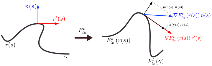
Figure 1: The evolution of material line $\gamma$ as well as its tangent and normal vectors under the linearized flow map $DF_{t_{0}}^{t}$.

The averaged Lagrangian shear experienced by $\gamma$ over the time interval $\left[t_{0},t\right]$ is given by [13]

$$P(\gamma)=\intop_{\gamma}p(r(s),r^{\prime}(s))ds=\intop_{\gamma}\sqrt{\frac{\left\langle r^{\prime}(s),D_{t_{0}}^{t}(r(s))r^{\prime}(s)\right\rangle}{\left\langle r^{\prime}(s),C_{t_{0}}^{t}(r(s))r^{\prime}(s)\right\rangle\left\langle r^{\prime}(s),r^{\prime}(s)\right\rangle}}ds.$$

We seek shearless LCSs as material lines with no leading order variation in their averaged Lagrangian shear. On the time $t_{0}$ position of such LCSs, the first variation of $P$ must necessarily vanish, i.e.,

$$\delta P(\gamma)=0.$$ (8)

The most readily observed solutions of (8) are those obtained under the largest possible set of admissible variations, including changes to the endpoints of $\gamma$. As shown in [13], the variational problem (8) posed with free-endpoint boundary conditions is equivalent to finding null-geodesics connecting singularities of the Lorentzian metric

$$g(u,v)=\left\langle u,D_{t_{0}}^{t}(x_{0})v\right\rangle,$$

where $\left\langle.,.\right\rangle$ denotes the Euclidean inner product. The singularities of $g(u,v)$ are points where $\det D_{t_{0}}^{t}(x_{0})=0$. These are precisely the points where the Cauchy–Green tensor field $C_{t_{0}}^{t}(x_{0})$ has repeated eigenvalues. Following the convention in the tensor-line literature [11], we refer to such points as the singularities of the Cauchy–Green strain tensor (Fig. 2).

All null-geodesics of the metric $g$ are found to be solutions of one of the two ODEs

$$r^{\prime}(s)=\xi_{j}(r(s)),\qquad j=1,2.$$ (9)

We refer to trajectories of (9) with $j=1$ as shrink lines, as they are compressed by the flow. Similarly, we call trajectories of (9) with $j=2$ stretch lines, because they are stretched by the flow. Shrink and stretch lines are special cases of tensor lines used in the scientific visualization literature to illustrate features of two-dimensional tensor fields [11].

Smooth null-geodesics connecting metric singularities of $g(u,v)$ are, therefore, smooth heteroclinic chains formed by shrink lines and stretch lines among the singularities. For observable impact on mixing, we focus on such null-geodesic chains that are structurally stable and locally unique. This requirement restricts the shrink-stretch chains of interest to those along which wedge- and trisector-type singularities of $C_{t_{0}}^{t}(x_{0})$ alternate (cf. Fig. 2 and [13] for details).

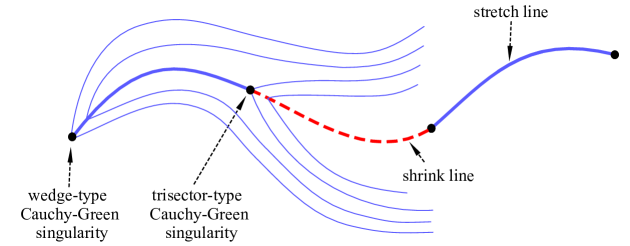
(a)

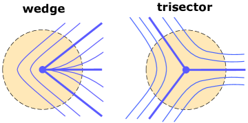
(b)

Figure 2: (a) A parabolic LCS is a structurally stable, alternating chain of shrink-stretch curve segments that connect Cauchy–Green singularities. A single shrink line (red) in such a chain is superimposed on the local stretch-line geometry (blue) near the LCS. (b) Topology of stretch lines around wedge-type and trisector-type Cauchy–Green singularities.

The time $t_{0}$ positions of parabolic LCSs (Lagrangian jet cores) are defined as tensor-line chains of the type in Fig. 2 that are also weak minimizers of a quantity that measures the closeness of the chain to being neutrally stable under advection by $F_{t_{0}}^{t}$ [13]. This quantity, the neutrality of a tensorline at a point $r$, is defined as

$$\mathcal{N}_{\xi_{j}}(r)=\left(\sqrt{\lambda_{k}(r)}-1\right)^{2},\qquad j\neq k.$$ (10)

A weak minimizer of $\mathcal{N}_{\xi_{j}}$ is then defined as a trajectory of (9) that lies, together with the nearest trench of $\mathcal{N}_{\xi_{j}}(r)$, in the same connected component of the set of points defined by the relation $\mbox{$\left\langle\nabla^{2}\mathcal{N}_{\xi_{j}}(r)\xi_{k}(r),\xi_{k}(r)\right\rangle$}>0$, with $j\neq k.$ (cf. [13] for more detail).

Figure 3 illustrates the construction of the time $t_{0}$ position of a parabolic LCS. The position of such an LCS at an arbitrary time $t$ can be found by advecting its $t_{0}$ position under the flow map $F_{t_{0}}^{t}$. Details on the numerical procedures involved can be found in [13].

The resilience of parabolic LCSs (serving as solutions to (8) even under variations to their endpoints) is in agreement with several numerical studies pointing out the robustness and easy observability of Lagrangian jet cores in unsteady zonal flows [44, 45, 6]. For a general discussion of importance of jet cores and their impact on global weather patterns, see [16].

Finally, time $t_{0}$ positions of hyperbolic LCSs are defined as Cauchy-Green tensorlines starting from local extrema of the strain-eigenvalue fields $\lambda_{i}(x_{0})$ [13, 23]. Hyperbolic LCSs, therefore, are also solutions of the stationarity principle (8) for shearless LCSs, but only with respect to variations leaving their endpoints fixed. This constraint on boundary conditions implies a lower degree of observability for hyperbolic LCSs relative to parabolic LCSs. Furthermore, in the short-time, shear-dominated context of the Jupiter video studied here, we have only found weak normal repulsion and attraction along material lines. We therefore omit a discussion of hyperbolic LCSs in this study.

(a)

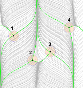
(b)

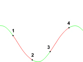
(c)

Figure 3: The construction of the initial position of a parabolic LCS for the standard non-twist map (cf. [13]). (a) Topology of shrink lines around wedges (singularities 1 and 3) and trisectors (singularities 2 and 4). Shrink-line separatrices are shown in red. (b) Topology of stretch lines around singularities. Stretch-line separatrices are shown in green. (c) Parabolic LCSs formed by a smooth shrink-stretch separatrix chain that is a weak minimizer of the neutrality (10).

3.2 Elliptic LCSs

By Fig. 1, the averaged Lagrangian repulsion experienced by a closed material curve $\gamma$ over the time interval $\left[t_{0},t\right]$ is given by

$$Q(\gamma)=\oint\displaylimits_{\gamma}q(r(s),r^{\prime}(s))ds=\oint\displaylimits_{\gamma}\frac{1}{\sqrt{\left\langle r^{\prime}(s),\left[C_{t_{0}}^{t}(r(s))\right]^{-1}r^{\prime}(s)\right\rangle\left\langle r^{\prime}(s),r^{\prime}(s)\right\rangle}}ds.$$ (11)

To generalize the concept of a Kolmogorov–Arnold–Moser-type (KAM-type) transport barrier [2] from time-periodic to finite-time aperiodic flows, we seek closed material curves $\gamma$ along which the averaged repulsion $Q$ shows no leading-order variation. Satisfying

$$\delta Q(\gamma)=0,$$ (12)

such a closed curve $\gamma$ has a thin annular neighborhood in which no material filamentation occurs over the time interval $[t_{0},t]$, just as in neighborhoods of KAM curves in the time-periodic case. As a result, the interior of $\gamma$ exhibits no advective mixing with its exterior. The observability of solutions of (12) is on par with those of (8). Indeed, they prevail under the largest possibly set of admissible variations, as long as those variations are also closed curves.

For incompressible flows, stationarity of the averaged normal repulsion is equivalent to the stationarity of the averaged tangential stretching defined along the material line $\gamma$. As shown in [24], the latter problem is solved by closed null-geodesics of the Lorentzian metric family

$$g_{\lambda}(u,v)=\left\langle u,E_{\lambda}v\right\rangle,\quad\lambda>0,$$

with the generalized Green–Lagrange strain tensor $E_{\lambda}(x_{0})$ defined as

$$E_{\lambda}(x_{0})=\frac{1}{2}\left[C_{t_{0}}^{t}(x_{0})-\lambda^{2}I\right].$$

The metric $g_{\lambda}$ is Lorentzian (i.e., indefinite) on the set $U_{\lambda}=\left\{x_{0}\in U\,:\,\lambda_{1}(x_{0})<\lambda^{2}<\lambda_{2}(x_{0})\right\}.$ In this set, all closed null-geodesics of $g_{\lambda}$ are trajectories of one of the two families of ODEs

$$r^{\prime}(s)=\eta_{\lambda}^{\pm}(r(s)),\qquad\lambda\in\mathbb{R}^{+},$$ (13)

where

$$\eta_{\lambda}^{\pm}(r) =\sqrt{\frac{\lambda_{2}(r)-\lambda^{2}}{\lambda_{2}(r)-\lambda_{1}(r)}}\xi_{1}(r)\pm\sqrt{\frac{\lambda^{2}-\lambda_{1}(r)}{\lambda_{2}(r)-\lambda_{1}(r)}}\xi_{2}(r).$$

Again, for reasons of observability, we focus on structurally stable closed trajectories (i.e., limit cycles) of (13).

Time $t_{0}$ positions of elliptic LCSs are, therefore, limit cycles of the line fields (13). Such limit cycles turn out to encircle at least two wedge-type singularities of the Cauchy–Green strain tensor field (Fig. 4). This fact enables the automated numerical detection of elliptic LCS even in complex flow fields [30].

The position of an elliptic LCS at an arbitrary time $t$ can be found by advecting its $t_{0}$ position under the flow map $F_{t_{0}}^{t}$. Any limit cycle $\gamma$ of (13) turns out to be uniformly stretching under such advection [24]. This means that the arclength of any subset of $\gamma$ increases exactly by the factor $\lambda$ under the flow map $F_{t_{0}}^{t}$. Limit cycles of (13) only tend to exist for $\lambda\approx 1$, guaranteeing a high degree of material coherence for a coherent Lagrangian vortex boundary, defined in [24] as the outermost member of a nested family of limit cycles of (13).

Figure 4 illustrates the construction of the time $t_{0}$ slice of an elliptic LCSs and coherent Lagrangian vortex boundaries. Details on the numerical procedures involved can be found in [24].

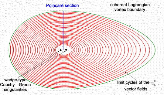
Figure 4: The construction of a Lagrangian vortex boundary for the periodically forced Duffing oscillator [21]. Elliptic LCSs are identified as limit cycles of the $\eta_{\lambda}^{\pm}$ direction fields via a Poincare section. The outermost elliptic LCS is highlighted with green as the Lagrangian vortex boundary.

4 Unsteady transport barriers in the atmosphere of Jupiter

4.1 Prior work and present objectives

Notable earlier attempts to identify transport barriers in Jupiter’s atmosphere from images started in [12], with velocities inferred from a manually assisted image-correlation analysis of 10 pairs of photos. The resulting velocities were then all viewed as part of an underlying steady wind field. This steady vector field produced spiraling streamlines near the GRS without a clear indication of material barriers.

Later work [9] used three high-resolution snapshots from the 2000 Galileo Mission to construct a steady velocity field from automated cloud-tracking via image correlation velocimetry. Again, trajectories spiraling into the GRS emerged from this time-averaged analysis, indicating no particular closed material barrier around the GRS. More recently, a potential-vorticity-conserving flow (steady in the frame co-moving with the GRS) was constructed in [48] as a best fit to cloud motion inferred from different space missions. By construction, this averaged approach renders all streamlines closed near a vortical feature (such as the GRS). The approach, however, does not address the question of actual material transport via the unsteady winds of Jupiter.

Extracting an unsteady velocity field and analyzing its finite-time transport barriers has not been attempted in prior publications. One reason for this is a clear focus of the planetary science community on long-term evolution in Jupiter’s climate. Comparing velocity snapshots and averages taken from different missions and different years, rather than studying a video footage from a single mission, is clearly more appropriate for a study of climate evolution. The unavoidable time-dependence of velocities extracted from temporally close video frames has, in fact, been viewed as undesirable uncertainty to an envisioned steady mean velocity field (see, e.g., Asay-Davis et al. [3]). Another reason for the lack of unsteady transport barrier studies for Jupiter has been the unavailability of precise mathematical tools (such as those surveyed here in Section 3) for LCS extraction from finite-time, aperiodic velocity data.

4.2 Video footage

The raw footage acquired by the Cassini Orbiter comprises 14 cylindrical maps of Jupiter, covering the 10 days ranging from October 31 to November 9 in the year 2000. We use an enhanced version of this video, which NASA created by interpolation and by addition of information from previous Jupiter missions [55, 56]. The pixels of the enhanced footage extend to 360 degrees of longitude and 180 degrees of latitude, with a resolution of $3601\times 1801$. The time step between the frames is 1.1 hours.

To verify the feasibility of the enhanced cloud movie for Lagrangian advection studies, we used the extracted velocity field (to be described below) to advect the first image of the raw footage up to the final time of the same footage. We show representative portions of these two images in Fig. 5 for comparison. We computed an offset error as the $l^{2}$-distance between the pixels of the advected initial raw image and the raw image at the final time, normalized by the $l^{2}$-norm of the final raw image. In this fashion, we obtained an offset error of $5.6\%$, which is in the order otherwise expected from numerical noise, processing errors, and diffusive cloud mixing.

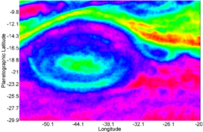
(a)

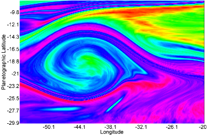
(b)

Figure 5: (a) Final frame of the raw footage. The image is shown in Hue-Saturation-Value (HSV) colormap. (b) The first frame of the raw footage is advected to the final time using the extracted velocity field.

4.3 Optical velocity field reconstruction

Image-correlation analysis applied to available cloud videos provides a two-dimensional representation of Jupiter’s winds. Early wind-field reconstruction studies required a human operator to identify the same cloud feature in subsequent frames [39]. The seminal paper by Limaye [34] introduced the first automated image-correlation method using one-dimensional correlations along latitudinal circles. Later improvements involved two-dimensional extensions and coarse-to-fine iteration schemes [8]. Recent approaches add an advection equation to the procedure [3], or apply the idea of an optical flow [35]. Similar methods have also been applied to image sequences of other planets such as Saturn [46], Uranus and Neptune [31], and the Earth [32].

Here we use the Advection Corrected Correlation Image Velocimetry (ACCIV) algorithm developed in [3] to extract a time-resolved atmospheric velocity field from the enhanced Cassini footage described in section 4.2. ACCIV uses the idea of the two-pass Image Correlation Velocimetry (CIV) developed by [52, 14, 15] for experimental fluid velocity measurement. In [3], the ACCIV algorithm was employed to reconstruct steady velocity fields from image pairs provided by the Hubble Space Telescope, as well as by the Galileo and Cassini space missions. To our knowledge, however, the ACCIV algorithm has not been employed before to reconstruct and analyze a time-resolved, unsteady velocity field from a full video footage.

ACCIV is an iterative technique for reconstructing a velocity field that is assumed to advect an observed scalar field passively. As a first step, ACCIV recursively splits two successive images $I$ and $J$ into sub-images or correlation boxes. Then, for a correlation box $C_{i}\subset I$, ACCIV finds a matching box $C_{j}\subset J$ of the same size. The process of matching correlation boxes is performed by maximizing the cross-correlation between intensity patterns. The velocity at the center of $C_{i}$ is then the distance between the centers of $C_{i}$ and $C_{j}$ divided by the time elapsed.

The algorithm repeats this process for all the correlation boxes in the image $I$, yielding a crude velocity field approximation under the assumption that a correlation box moves from image $I$ to the subsequent image $J$ without any distortion. The crude initial velocity approximation is then used to advect the images to some intermediate time when no real data are available. The difference between the synthetic images at the intermediate time is iteratively used to generate correction vector fields, producing increasingly accurate velocity vectors. In a second step, ACCIV makes use of the first-step results and looks for a correlation between a box of pixels in the image $I$ and a box of pixels transformed in the subsequent image $J$. The possible transformations are a combination of translation, rotation, shear and distortion. Figure 6 illustrates how considering a deformed correlation box can lead to a better approximation of the displacement vector at the center of the correlation box $C_{i}$. Similar to the first step, ACCIV iteratively improves the accuracy of the velocity vectors by building synthetic images and producing correction vectors. The next steps consist of further refinement of the velocity field using smaller correlation boxes.

ACCIV first pass

(a)

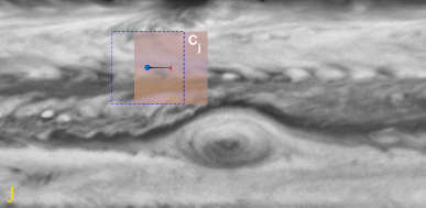
(b)

ACCIV second pass

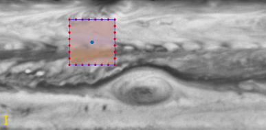
(c)

(d)

Figure 6: Correlation boxes in the first and second ACCIV passes. (a) A correlation box of pixels $C_{i}$ in image $I$ is shown as a solid line. (b) The matching correlation box $C_{j}$ in the subsequent image $J$ is shown along the silhouette of the correlation box $C_{i}$. The black arrow connecting the centers of the correlation boxes shows the estimated displacement vector at the center of $C_{i}$. The displacement vector is obtained under the assumption that $C_{i}$ moves from image $I$ to $J$ without any distortion. (c) The correlation box of pixels $C_{i}$ at initial image $I$. (d) The distorted matching correlation box in the image $J$. The given freedom to the correlation box $C_{i}$ leads to a better estimation of the displacement vector (shown in black).

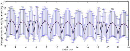
Figure 7: The average correlation velocity uncertainty as a percentage of the spatial mean of the reconstructed velocities is shown in black for each video frame. The standard deviation of velocity uncertainty data is shown in blue.

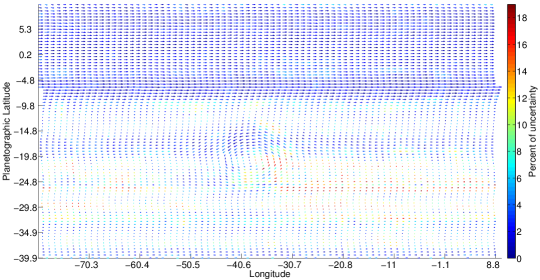
Figure 8: The correlation velocity uncertainty is shown as a percent of velocity magnitude at the location of velocity grid points. The result is shown for the frame number 105.

ACCIV repeats each of these steps iteratively until the velocity correlation uncertainty shows no further decrease. First, ACCIV defines the offset between advected and raw images at time $t_{2}$ as local correlation location uncertainty. The correlation velocity uncertainty is then the correlation location uncertainty divided by the time elapsed between the images. The velocity fields we have extracted with ACCIV have tens to hundreds of thousands of independent velocity vectors with uncertainties on the order of 2-5 $m/s$.

Figure 7 shows the measure of correlation velocity uncertainty as a percentage of the spatial mean velocity for each video frame. The near-periodicity of the uncertainty history arises from the mostly even sampling frequency (roughly two jovian days) of the original raw footage from Cassini. Two time intervals (around days 5-7 and 16-18) with shorter sampling times create an impression of approximate symmetry in the uncertainty distribution with respect to day 12, but this is accidental.

On average, the extracted velocity vectors have about $6.4\%$ uncertainty with respect to the mean of the reconstructed velocities. Figure 8 shows the spatial distribution of velocity uncertainty as a percentage of the velocity norm at each grid point. The velocity uncertainty is higher in regions such as the GRS where we have complicated dynamics and presumably cloud mixing.

We recall that we integrate the reconstructed velocity field to find structurally stable structures: limit cycles for elliptic LCSs and robust heteroclinic cycles for parabolic LCSs (cf. Section 3). These structures persist in the (unknown) true velocity field, as long as the imaging and reconstruction errors represent an overall moderate perturbation to the flow map, such as the perturbation we infer from Fig. 5. This persistence result holds even if the velocity errors are pointwise large at times (cf. [25]).

Some input parameters for ACCIV, such as the times between frames and the threshold for removing outliers, are straightforward to specify. Other parameters, such as correlation box size, search range, and stride, must be optimized iteratively. Table 1 summarizes the input parameters and results for each pass. For more information on setting the input parameters of ACCIV, we refer the reader to the project webpage [58].

Table 1: ACCIV parameters used to produce the time-resolved velocity field. The box size, search range, and stride are in units of pixels. The box size is the size of the correlation box for the relevant CIV pass. The search range is the range of correlation box displacements used in each dimension. The stride is the number of pixels by which the correlation box is shifted between each measurement. It controls the output resolution of the velocity vector field. The number of image pairs is the total number of pairing of the set of images. The Number of Smooth Fit Control Point Neighbors controls the smoothness of the velocity field on the grid.

Figure 9 shows a representative snapshot of the reconstructed unsteady velocity field, which is available over the domain ranging from $-180\,^{\circ}{\rm W}$ to $180^{\circ}{\rm E}$ in longitudes and from $-35^{\circ}{\rm S}$ to $20^{\circ}{\rm N}$ in latitudes, with a grid resolution of $7202\times 1102$. This supersedes the resolution of earlier velocity fields reconstructed for Jupiter from manual cloud-tracking approaches [39, 12, 49, 33, 53].

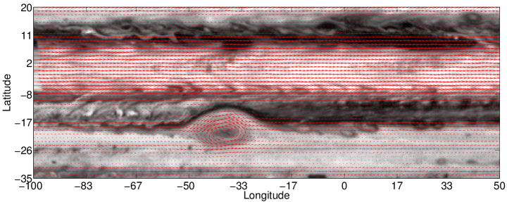
Figure 9: A representative snapshot (frame number 105) of the unsteady velocity field using the ACCIV algorithm. Only one tenth of the total number of velocity vectors are shown for the sake of visual clarity.

In principle, an alternative to the ACCIV method used here would be Digital Particle Image Velocimetry (DPIV), which reproduces fluid velocities from highly resolved tracks of luminescent particles in well-illuminated laboratory flows [26]. Under such conditions, high-speed imaging can reliably detect small particle displacements amidst minimal illumination changes, a basic requirement for the optical flow methods underlying DPIV. In observations of planetary atmospheres, however, these ideal imaging conditions are generally not met. For instance, the sunlight scattered from Jupiter’s cloud cover into the camera of a spacecraft tends to vary considerably between two subsequent images.

As a consequence, optical flow methods have not gained popularity in velocity field reconstruction from planetary observations. A rare exception is Ref. [35], which works with a single pair of well-lit, high-resolution images from NASA’s Galileo mission, separated by one hour. From this data, [35] extracts a single high-quality, steady velocity snapshot. Unfortunately, the data available from the Galileo mission is insufficient for the extraction of a reasonably long unsteady velocity field via the approach of [35].

In comparison to the two high-resolution images used in [35], the more modestly resolved but temporally extended Cassini data set used here offers a clear advantage for unsteady LCS detection. As is now well-established for satellite altimetry maps of the ocean, even without capturing smaller (sub-mesocale and lower) features of a velocity field, one can accurately capture its mesoscale LCSs, which in turn agree with in situ float observations [40].

4.4 Validation of the reconstructed velocity field

Available observational records of Jupiter go back to the late 19th century, indicating that Jupiter’s atmosphere is highly stable in the latitudinal direction. The average zonal velocity profile as a function of latitudinal degree is, therefore, an important benchmark in assessing the quality of the reconstructed velocity field.

In Fig. 10, we compare the temporally averaged zonal velocity profile obtained from ACCIV with the classic profile reported by Limaye [34]. The Limaye profile has been used and confirmed by several other studies on different data sets from different missions (see, e.g., [27, 53, 18]). These studies all support the conclusion that the averaged zonal wind field constructed by Limaye [34] has remained fundamentally unaltered.

Limaye’s velocity profile is based on Voyager I and Voyager II images, covering a total of 142 Jovian days in 1979. In contrast, our ACCIV-based velocity profile is based on the Cassini mission, and covers a total of 24 Jovian days in 2000-2001 [55]. Overall, the two profiles shown in Fig. 10 match fairly closely, showing only appreciable discrepancies near velocity extrema. These discrepancies arise because ACCIV, as other image-correlation methods, systematically underestimates the magnitude of the velocity vectors near peaks of the velocity field [3].

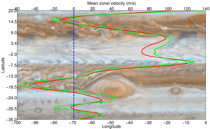
(a)

Figure 10: Zonal velocity profile of Jupiter’s atmosphere. The red line represents the average obtained from the reconstructed velocity field; the green profile is the one reported by S.S. Limaye [34]. The Cassini map PIA07782 is used as background.

We finally note that we have used images taken at the visible wavelength to extract the velocities of Jupiter’s clouds. Asay-Davis et al., [4] show that velocities extracted from images taken with different visible wavelengths (at different times) produce similar zonal velocities. This observation and other empirical studies support the expectation that Jupiter’s cloud velocities can be correctly inferred from images taken at visible wavelengths.

4.5 Lagrangian advection

For the parabolic LCS computation described in section 3.1, we calculate the Cauchy–Green strain tensor field $C_{t_{0}}^{t}$ defined in (3) with $t_{0}=0$ and $t=24$ days, over a uniform grid $\mathcal{G}_{0}^{1}$ of $5600\times 2200$ points. The spatial domain $U$ ranges from $-145\,^{\circ}{\rm W}$ to $95^{\circ}{\rm E}$ in longitudes and from $-35^{\circ}{\rm S}$ to $20^{\circ}{\rm N}$ in latitudes. For the elliptic LCS computations described in section 3.2, a smaller grid $\mathcal{G}_{0}^{2}$ of $900\times 600$ points suffices, because the accurate identification of Cauchy–Green singularities is not crucial. In all computations, we use a variable-order Adams–Bashforth–Moulton solver (ODE113 in MATLAB) to solve the differential equations (1) and (13). The absolute and relative tolerances of the ODE solver are chosen as $10^{-6}$. Off the grid points, we obtain the $\xi_{j}(x_{0})$ and $\eta_{\lambda}^{\pm}(x_{0})$ line fields from bilinear interpolation.

4.6 Unsteady zonal jet cores as parabolic LCSs

Influential work on model flows has indicated that high potential-vorticity (PV) gradients occurring along the cores of the eastward jets of Jupiter create effective barriers to material transport [28]. More recent work on perturbed PV-staircase flow models revealed that westward jet cores also act as material barrier cores, even when the PV has vanishing gradients along these lines [6]. Averaged meridional velocities support this conclusion [6], but time-resolved studies using observed winds have not been carried out to ascertain the existence of actual material transport barriers along eastward and westward jet cores.

Here we examine the validity of the above model-based conclusions on the unsteady wind field inferred from the time-resolved Cassini footage. Applying the theory surveyed in section 3.1, we compute the Lagrangian cores of jet streams located between latitudes $-35\,^{\circ}{\rm S}$ and $20\,^{\circ}{\rm N}$ (see Fig. 11a). In line with the model-based conclusions of [6], we find coherent Lagrangian jet cores both for eastward and westward jets. Unlike the straight lines suggested by individual snapshots, however, the actual unsteady jet cores exhibit small-amplitude north-south oscillations, as shown in Fig. 11b.

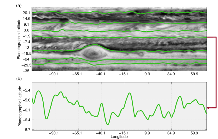
Figure 11: (a) Instantaneous positions of parabolic LCSs at the initial time as shearless transport barriers that form the core of jet streams in the atmosphere of Jupiter. (b) The spatial profile of Jupiter’s southern equatorial jet. The average meandering width is about $0.33\,^{\circ}$ latitudinal degree.

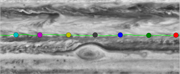
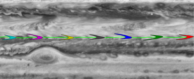
Figure 12: Impact of Jupiter’s southern equatorial shearless transport barrier on tracer disks over 11 jovian days. The deformed tracer disks resemble the shape of the recently discovered chevrons [49], i.e., dark v-shaped clouds in the background. The contrast of images is improved for better visualization. The complete advection sequence over 24 Jovian days is illustrated in the online supplemental movie M1.

Figure 12 shows the evolution of initially circular blobs of tracers, centered on the shearless core of the southern equatorial jet, after 11 Jovian days. The shape of tracer blobs resembles the shape of chevrons, serving as Lagrangian footprints of Rossby waves identified recently from an Eulerian perspective on the southern hemisphere of Jupiter [49].

The advected jet core, as a material line, does not allow mixing between the two wings of any chevron. Specifically, the evolving parabolic LCS does act as a transport barrier, keeping its coherence, and showing no wave-breaking or fingering-type deformation. This coherence effectively blocks the advective excursion of material between the upper and lower half of the material jet.

4.7 The Great Red Spot as a generalized KAM region

Observational evidence suggests the existence of coherent rings around all jovian vortices, including the GRS. The accepted explanation is that these rings are signs of vertically moving air parcels in the three-dimensional atmosphere of the planet [10, 41]. A ring of air parcels is a material transport barrier that is expected to have a two-dimensional footprint in the horizontal wind field around the GRS. Such a signature, however, has not been identified in available advection studies (cf. section 4.1)

Here we seek an annular material transport barrier region around the GRS by applying the geodesic LCS theory described in section 3.2. This necessitates the computation of limit cycles for the family of autonomous dynamical systems defined in eq. (13). We discard limit cycles obtained for the same $\lambda$ value, if they are within two velocity grid steps from each other. This is to focus on robust enough limit cycles that are far enough from undergoing a saddle-node bifurcation.

This computation yields 73 elliptic LCSs, computed as robust limit cycles of the differential equation family (13) (Fig. 13a). This set of closed curves forms a generalized KAM region, filled with material loops that resist filamentation and act as coherent transport barriers through the entire duration of the underlying video footage.

Figure 13b shows separately the elliptic LCS with perfect coherence ($\lambda=1$) in black, as well as the outermost elliptic LCS in blue that forms the outer boundary of the coherent Lagrangian vortex associated with the GRS. This vortex boundary is marked by the parameter value $\lambda=1.0063$, which forecasts a roughly $0.6\%$ increase in arclength. The two closed curves enclose a highly coherent annular barrier, the Lagrangian counterpart of the outer ring identified within a collar of the GRS described in [35]. This outer ring was constructed as the annulus outside the perceived core of the collar, a closed curve of velocity maxima.

Our geometric construction of an annular Lagrangian transport barrier is also motivated by the visual observations in [41]. These often indicate a sharper inner boundary and a more diffusive outer boundary for coherent jovian rings. The sharp observational boundary suggests an elliptic LCS of the highest possible coherence (zero stretching), while a diffusive outer boundary is expected near an elliptic LCS of the lowest possible coherence (highest stretching in a family of elliptic LCSs).

The exact location of these oval barriers is expected to change under varying data resolution. The structural stability in the construction of elliptic LCSs, however, guarantees that the barriers move only by a small amount under small enough variations in resolution.

Advected images of the extracted GRS boundary confirm its sustained coherence over the finite time of extraction (see Figures 13c, 13d and 13e). Our computation shows that the predicted coherent core of the GRS indeed regains its arc-length after 24 Jovian days. At the same time, the coherent outer boundary of the GRS indeed grows in arclength by about $0.6\%$, while its longitudinal extent decreases by about $5\%$. This suggests that the coherent boundary of the GRS is becoming rounder, which is generally consistent with the available observational records taken over much longer periods [50] (see Fig. 13f). Clearly, any firm conclusion or prediction about the long-term behavior of the arclength of material GRS boundary would require the analysis of a substantially longer data set.

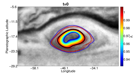
(a)

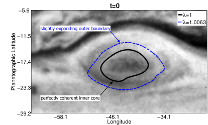
(b)

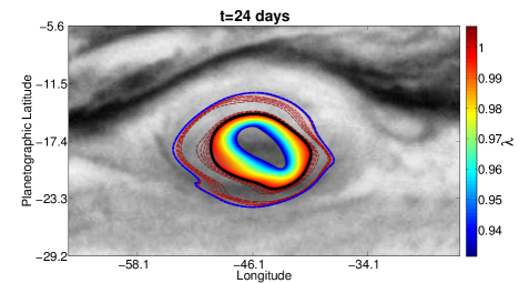
(c)

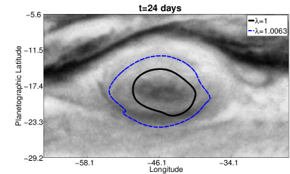
(d)

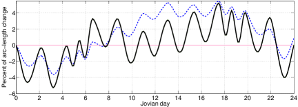
(e)

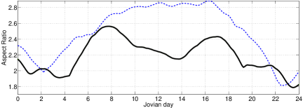
(f)

Figure 13: (a) Elliptic LCSs defining the Lagrangian footprint of the Great Red Spot at time $t=0$. The color-bar refers to values of the stretching parameter $\lambda$ arising in the construction of the elliptic LCS family. (b) Elliptic LCS with perfect coherence (black), as well as the Lagrangian vortex boundary (blue) of the Great Red Spot at time $t=0$. The boundary is extracted from velocity data covering 24 Jovian days. The advection sequence is illustrated in the online supplemental movie M2. (c) Elliptic LCSs defining the Lagrangian footprint of the Great Red Spot at time $t=24$. (d) Elliptic LCS with perfect coherence (black), as well as the Lagrangian vortex boundary (blue) of the Great Red Spot at time $t=24$. (e) Relative stretching of the perfectly coherent ($\lambda=1$) inner-core boundary and the slightly expanding outer boundary of the GRS over 24 Jovian days. As predicted by geodesic theory, the arc-length of the outer boundary changes about $0.6\%$ in agreement with the theoretical stretching value $(\lambda=1.0063$) of the extracted outer boundary. (f) plot of aspect ratio $(length^{2}/area)$ as a function of time.

5 Summary

We have applied the recently developed geodesic theory of transport barriers [24, 13] to an enhanced video from NASA’s Cassini mission to Jupiter. First, we obtained a representative two-dimensional wind field from this video via the Advection Corrected Correlation Image Velocimetry (ACCIV) algorithm of Asay–Davis et al. [3]. Next, we identified, for the first time, unsteady material transport barriers in the wind field that form the cores of zonal jets and the boundary of the Great Red Spot (GRS) in Jupiter’s atmosphere.

The parabolic LCSs (Lagrangian jet cores) we have found show that both easterly and westerly jet cores provide strong material transport barriers. This latter finding confirms the conclusion of Beron-Vera et al. [6] based on a numerical study of a perturbed potential-vorticity-staircase model relevant for Jupiter. Deforming material blobs placed near the parabolic LCS also reveal the Lagrangian footprint of the recently discovered chevron-type atmospheric features [49].

The elliptic LCSs we identify provide a foliation of the GRS into highly coherent, uniformly stretching layers. This supports the existence of a proposed two-dimensional, cylindrical material transport barrier around the GRS [10, 41]. According to our results, this cylindrical region has finite width, represented by an annulus in our two dimensional analysis. The annulus has a perfectly coherent ($\lambda=1$) inner boundary and a nearly perfectly coherent outer boundary, as shown in Fig. 13b. While the outer boundary shrinks in longitudinal extent over the observed 24 Jovian days, its total arc-length shows a slight increase of about $0.6\%$. This suggests a modest evolution of this Lagrangian boundary towards more perfect circularity, which is in line with longer observational records [50].

The time-resolved image reconstruction technique employed here is purely kinematic, and does not incorporate a fit to dynamic equations believed to govern Jupiter’s wind fields. Considerable effort has been devoted to fitting dynamically consistent reduced models to optically reconstructed velocities (see, e.g., [48]). These models, however, are steady in a moving frame, and incorporate velocity measurements from different sources and times. Here, instead of securing dynamical consistency for an averaged, steady velocity field, we have constructed an unsteady velocity field that is kinematically consistent with a specific observational period. Imposing some degree of dynamical consistency on the optically reconstructed velocity field and comparing it with steady models in a moving frame remains a viable future research direction. A clear challenge is that the cloud distribution over the GRS does not align with the location of its associated potential vorticity anomaly or with any other of the GRS’s known dynamical features [3].

Arriving at Jupiter in 2016, the Juno mission of NASA will explore some of the material movement deep beneath the planet’s clouds for the first time [57]. Using this future information, we expect to be able to extend some aspects of our present analysis to three-dimensions using recently developed 3D variational LCS methods [7].

We envision further applications of the methodology developed here to remotely observed patterns in meteorology [43], oceanography [5], environmental monitoring [54, 37] and crowd surveillance [1, 51].

References

- [1] S. ALI and M. SHAH, A Lagrangian particle dynamics approach for crowd flow segmentation and stability analysis, 2007 IEEE Conference on Computer Vision and Pattern Recognition, Vols 1-8 (2007), pp. 65-70.
- [2] V. I. ARNOLD, Mathematical Methods of Classical Mechanics, Springer, 1989.
- [3] X. S. ASAY-DAVIS, P. S. MARCUS, M. H. WONG and I. DE PATER, Jupiter’s shrinking Great Red Spot and steady Oval BA: Velocity measurements with the ’Advection Corrected Correlation Image Velocimetry’ automated cloud-tracking method, Icarus, 203 (2009), pp. 164-188.
- [4] X. S. ASAY-DAVIS, P. S. MARCUS, M. H. WONG and I. DE PATER, Changes in Jupiter’s zonal velocity between 1979 and 2008, Icarus, 211 (2011), pp. 1215-1232.
- [5] F. J. BERON-VERA, M. J. OLASCOAGA and G. J. GONI, Oceanic mesoscale eddies as revealed by Lagrangian coherent structures, Geophysical Research Letters, 35 (2008), L12603.
- [6] F. J. BERON-VERA, M. G. BROWN, M. J. OLASCOAGA, I. I. RYPINA, H. KOCAK and I. A. UDOVYDCHENKOV, Zonal jets as transport barriers in planetary atmospheres, Journal of the Atmospheric Sciences, 65 (2008), pp. 3316-3326.
- [7] D. BLAZEVSKI and G. HALLER, Hyperbolic and elliptic transport barriers in three-dimensional unsteady flows, Physica D-Nonlinear Phenomena, 273 (2014), pp. 46-62.
- [8] H. A. BRUCK, S. R. MCNEILL, M. A. SUTTON and W. H. PETERS, Digital Image Correlation Using Newton-Raphson Method of Partial-Differential Correction, Experimental Mechanics, 29 (1989), pp. 261-267.
- [9] D. S. CHOI, D. BANFIELD, P. GIERASCH and A. P. SHOWMAN, Velocity and vorticity measurements of Jupiter’s Great Red Spot using automated cloud feature tracking, Icarus, 188 (2007), pp. 35-46.
- [10] B. J. CONRATH, F. M. FLASAR, J. A. PIRRAGLIA, P. J. GIERASCH and G. E. HUNT, Thermal Structure and Dynamics of the Jovian Atmosphere .2. Visible Cloud Features, Journal of Geophysical Research-Space Physics, 86 (1981), pp. 8769-8775.
- [11] T. DELMARCELLE and L. HESSELINK, Visualizing 2nd-order tensor-fields with hyperstreamlines, IEEE Computer Graphics and Applications, 13 (1993), pp. 25-33.
- [12] T. E. DOWLING and A. P. INGERSOLL, Potential vorticity and layer thickness variations in the flow around jupiters great red spot and white oval bc, Journal of the Atmospheric Sciences, 45 (1988), pp. 1380-1396.
- [13] M. FARAZMAND, D. BLAZEVSKI and G. HALLER, Shearless transport barriers in unsteady two-dimensional flows and maps, Physica D-Nonlinear Phenomena, 278 (2014), pp. 44-57.
- [14] A. M. FINCHAM and G. R. SPEDDING, Low cost, high resolution DPIV for measurement of turbulent fluid flow, Experiments in Fluids, 23 (1997), pp. 449-462.
- [15] A. FINCHAM and G. DELERCE, Advanced optimization of correlation imaging velocimetry algorithms, Experiments in Fluids, 29 (2000), pp. S13-S22.
- [16] J. A. FRANCIS and S. J. VAVRUS, Evidence linking Arctic amplification to extreme weather in mid-latitudes, Geophysical Research Letters, 39 (2012).
- [17] G. FROYLAND, N. SANTITISSADEEKORN and A. MONAHAN, Transport in time-dependent dynamical systems: Finite-time coherent sets, Chaos, 20 (2010), 043116.
- [18] E. GARCI and A. SANCHEZ-LAVEGA, A study of the stability of jovian zonal winds from HST images: 1995-2000, Icarus, 152 (2001), pp. 316-330.
- [19] G. S. GOLITSYN, Similarity approach to general circulation of planetary atmospheres, Icarus, 13 (1970), pp. 1-8.
- [20] M. E. GURTIN, An Introduction to Continuum Mechanics, Elsevier Science, 1982.
- [21] A. HADJIGHASEM, M. FARAZMAND and G. HALLER, Detecting invariant manifolds, attractors, and generalized KAM tori in aperiodically forced mechanical systems, Nonlinear Dynamics, 73 (2013), pp. 689-704.
- [22] G. HALLER and G. YUAN, Lagrangian coherent structures and mixing in two-dimensional turbulence, Physica D, 147 (2000), pp. 352-370.
- [23] G. HALLER, Lagrangian Coherent Structures, Annual Review of Fluid Mechanics, 47 (2015), pp. 137-162.
- [24] G. HALLER and F. J. BERON-VERA, Coherent Lagrangian vortices: the black holes of turbulence, Journal of Fluid Mechanics, 731 (2013), R4.
- [25] G. HALLER, Lagrangian coherent structures from approximate velocity data, Physics of Fluids, 14 (2002), pp. 1851-1861.
- [26] D. HEITZ, E. MEMIN and C. SCHNORR, Variational fluid flow measurements from image sequences: synopsis and perspectives, Experiments in Fluids, 48 (2010), pp. 369-393.
- [27] A. P. INGERSOLL, R. F. BEEBE, J. L. MITCHELL, G. W. GARNEAU, G. M. YAGI and J. P. MULLER, Interaction of Eddies and Mean Zonal Flow on Jupiter as Inferred from Voyager-1 and Voyager-2 Images, Journal of Geophysical Research-Space Physics, 86 (1981), pp. 8733-8743.
- [28] M. N. JUCKES and M. E. MCINTYRE, A High-Resolution One-Layer Model of Breaking Planetary-Waves in the Stratosphere, Nature, 328 (1987), pp. 590-596.
- [29] D. KARRASCH, M. FARAZMAND and G. HALLER, Attraction-based computation of hyperbolic Lagrangian coherent structures, in press (2015).
- [30] D. KARRASCH, F. HUHN and G. HALLER, Automated detection of coherent Lagrangian vortices in two-dimensional unsteady flows, Proceedings of the Royal Society A-Mathematical Physical and Engineering Sciences, 470 (2015).
- [31] Y. KASPI, A. P. SHOWMAN, W. B. HUBBARD, O. AHARONSON and R. HELLED, Atmospheric confinement of jet streams on Uranus and Neptune, Nature, 497 (2013), pp. 344-347.
- [32] J. A. LEESE, C. S. NOVAK and B. B. CLARK, An Automated Technique for Obtaining Cloud Motion from Geosynchronous Satellite Data Using Cross Correlation, Journal of Applied Meteorology, 10 (1971), pp. 118-132.
- [33] J. LEGARRETA and A. SANCHEZ-LAVEGA, Jupiter’s cyclones and anticyclones vorticity from Voyager and Galileo images, Icarus, 174 (2005), pp. 178-191.
- [34] S. S. LIMAYE, Jupiter - new estimates of the mean zonal flow at the cloud level, Icarus, 65 (1986), pp. 335-352.
- [35] T. LIU, B. WANG and D. S. CHOI, Flow structures of Jupiter’s Great Red Spot extracted by using optical flow method, Physics of Fluids, 24 (2012), 096601.
- [36] T. MA and E. M. BOLLT, Differential Geometry Perspective of Shape Coherence and Curvature Evolution by Finite-Time Nonhyperbolic Splitting, SIAM Journal on Applied Dynamical Systems, 13 (2014), pp. 1106-1136.
- [37] D. MACKENZIE, Walls of Water, Scientific American, 309 (2013), pp. 86-89.
- [38] I. MEZIC, S. LOIRE, V. A. FONOBEROV and P. HOGAN, A New Mixing Diagnostic and Gulf Oil Spill Movement, Science, 330 (2010), pp. 486-489.
- [39] J. L. MITCHELL, R. F. BEEBE, A. P. INGERSOLL and G. W. GARNEAU, Flow-fields within jupiters great red spot and white oval bc, Journal of Geophysical Research-Space Physics, 86 (1981), pp. 8751-8757.
- [40] M. J. OLASCOAGA, F. J. BERON-VERA, G. HALLER, J. TRINANES, M. ISKANDARANI, E. F. COELHO, B. K. HAUS, H. S. HUNTLEY, G. JACOBS, A. D. KIRWAN, B. L. LIPPHARDT, T. M. OZGOKMEN, A. J. H. M. RENIERS and A. VALLE-LEVINSON, Drifter motion in the Gulf of Mexico constrained by altimetric Lagrangian coherent structures, Geophysical Research Letters, 40 (2013), pp. 6171-6175.
- [41] I. DE PATER, M. H. WONG, P. MARCUS, S. LUSZCZ-COOK, M. ADAMKOVICS, A. CONRAD, X. ASAY-DAVIS and C. GO, Persistent rings in and around Jupiter’s anticyclones - Observations and theory, Icarus, 210 (2010), pp. 742-762.
- [42] T. PEACOCK and J. DABIRI, Introduction to Focus Issue: Lagrangian Coherent Structures, Chaos: An Interdisciplinary Journal of Nonlinear Science, 20 (2010), 017501.
- [43] J. F. PENG and R. PETERSON, Attracting structures in volcanic ash transport, Atmospheric Environment, 48 (2012), pp. 230-239.
- [44] I. I. RYPINA, M. G. BROWN and F. J. BERON-VERA, On the lagrangian dynamics of atmospheric zonal jets and the permeability of the stratospheric polar vortex, Journal of the Atmospheric Sciences, 64 (2007), pp. 3595-3610.
- [45] I. I. RYPINA, M. G. BROWN, F. J. BERON-VERA, H. KOCAK, M. J. OLASCOAGA and I. A. UDOVYDCHENKOV, Robust transport barriers resulting from strong Kolmogorov-Arnold-Moser stability, Physical Review Letters, 98 (2007).
- [46] A. SANCHEZ-LAVEGA, T. DEL RIO-GAZTELURRUTIA, R. HUESO, J. M. GOMEZ-FORRELLAD, J. F. SANZ-REQUENA, J. LEGARRETA, E. GARCIA-MELENDO, F. COLAS, J. LECACHEUX, L. N. FLETCHER, D. BARRADO-NAVASCUES, D. PARKER and T. INT OUTER PLANET WATCH, Deep winds beneath Saturn’s upper clouds from a seasonal long-lived planetary-scale storm, Nature, 475 (2011), pp. 71-74.
- [47] S. C. SHADDEN, Lagrangian Coherent Structures, Transport and Mixing in Laminar Flows, Wiley-VCH Verlag GmbH & Co. KGaA, 2011, pp. 59-89.
- [48] S. SHETTY and P. S. MARCUS, Changes in Jupiter’s Great Red Spot (1979-2006) and Oval BA (2000-2006), Icarus, 210 (2010), pp. 182-201.
- [49] A. A. SIMON-MILLER, J. H. ROGERS, P. J. GIERASCH, D. CHOI, M. D. ALLISON, G. ADAMOLI and H.-J. METTIG, Longitudinal variation and waves in Jupiter’s south equatorial wind jet, Icarus, 218 (2012), pp. 817-830.
- [50] A. A. SIMON-MILLER, P. J. GIERASCH, R. F. BEEBE, B. CONRATH, F. M. FLASAR, R. K. ACHTERBERG and C. T. CASSINI, New observational results concerning Jupiter’s Great Red Spot, Icarus, 158 (2002), pp. 249-266.
- [51] A. SURANA, A. NAKHMANI and A. TANNENBAUM, Anomaly detection in videos: A dynamical systems approach, 2013 IEEE 52nd Annual Conference on Decision and Control (CDC) (2013), pp. 6489-95.
- [52] P. T. TOKUMARU and P. E. DIMOTAKIS, Image Correlation Velocimetry, Experiments in Fluids, 19 (1995), pp. 1-15.
- [53] A. R. VASAVADA, A. P. INGERSOLL, D. BANFIELD, M. BELL, P. J. GIERASCH, M. J. S. BELTON, G. S. ORTON, K. P. KLAASEN, E. DEJONG, H. H. BRENEMAN, T. J. JONES, J. M. KAUFMAN, K. P. MAGEE and D. A. SENSKE, Galileo imaging of Jupiter’s atmosphere: The Great Red Spot, equatorial region, and White Ovals, Icarus, 135 (1998), pp. 265-275.
- [54] X. WEI, P. T. NI and H. G. ZHAN, Monitoring cooling water discharge using Lagrangian coherent structures: A case study in Daya Bay, China, Marine Pollution Bulletin, 75 (2013), pp. 105-113.
- [55] http://ciclops.org/view.php?id=92&js=1
- [56] http://svs.gsfc.nasa.gov/goto?3610
- [57] http://www.nasa.gov/mission_pages/juno/overview/
- [58] https://code.google.com/p/acciv/wiki/OptimizingParameters