Event-by-event simulation of a quantum delayed-choice experiment
Abstract
The quantum delayed-choice experiment of Tang et al. [Nature Photonics 6 (2012) 600] is simulated on the level of individual events without making reference to concepts of quantum theory or without solving a wave equation. The simulation results are in excellent agreement with the quantum theoretical predictions of this experiment. The implication of the work presented in the present paper is that the experiment of Tang et al. can be explained in terms of cause-and-effect processes in an event-by-event manner.
keywords:
discrete event simulation , Wheeler delayed-choice experiment , interference , quantum optics1 Introduction
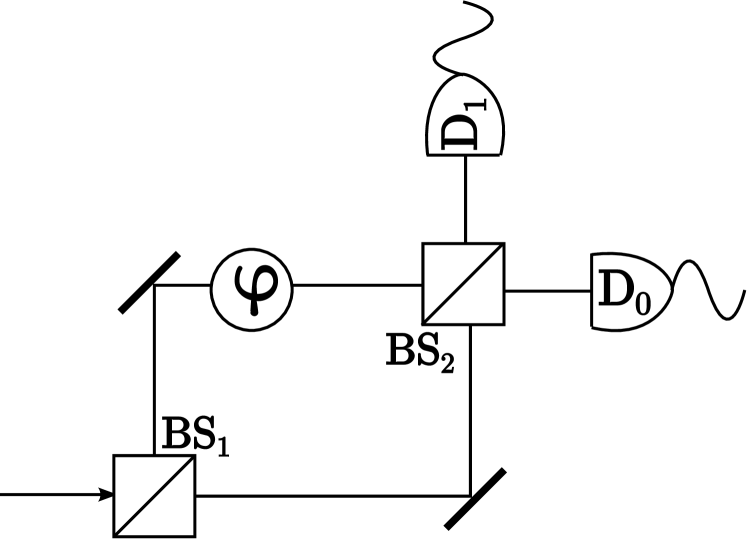
In a Mach-Zehnder interferometer (MZI) experiment one can choose between measuring the wave-like and the particle-like properties of photons [1, 2]. The wave-like behavior (interference) is observed using the MZI set-up depicted in Fig. 1. The particle-like behavior (no interference) is observed by removing the second beam splitter BS2. The first and second set-up are henceforth referred to as a closed and an open MZI, respectively. Hence, the observation of wave-like or particle-like behaviour depends on the choice of considering a closed or open MZI, respectively, in accordance with the idea of wave-particle duality. One might therefore ask whether a normal-choice and a delayed-choice experiment would yield different observations. That is, is there a difference in the experimental results if the set-up is already predetermined to test either the particle or wave nature of a photon (normal-choice) versus a set-up that makes this choice while the photon has already passed BS1 but not yet BS2 (delayed-choice)? Experiments have been carried out to measure this difference and there appears to be no difference between these two situations [3, 4, 5].
Recently, a new type of delayed-choice experiment has been suggested in which BS2 is a quantum beam splitter assumed to be in a superposition of being present and absent [6]. This so-called quantum delayed-choice experiment has been realized experimentally using NMR interferometry on ensembles of molecules [7, 8] and using single-photon quantum optics techniques [9, 10, 11]. These experiments demonstrate that in one single experiment, particle- or wave-like behavior can be tuned continuously, which is interpreted as an indication that the complementarity principle needs refinement [9, 10, 11].
From the viewpoint of quantum theory, the central issue is how it can be that experiments such as these delayed-choice experiments yield definite answers [12]. As the concept of an event is not a part of quantum theory proper, quantum theory simply cannot address the question “why there are events?” [13]. One can get around this conundrum by constructing a description entirely in terms of events, ultimately related to human experience, and the cause-and-effect relations among them. Such an event-based description obviously yields definite answers and if it reproduces the statistical results of experiments, it also provides a description of the experiments on a level of detail that is not covered by quantum theory.
Essentially, the event-based approach is based on the fact that all that what can be said about nature is constrained by the data a measurement apparatus can, at least in principle, produce. As Wheeler put it: “[…] every particle, every field of force, even the space-time continuum itself–derives its function, its meaning, its very existence entirely […] from the apparatus-elicited answers to yes-or-no questions […].” [14]. The event-based approach is to be viewed in this light; An event-based simulation does not necessarily mimic what actually happens in nature: it only produces sets of data (e.g. detector clicks) that can be compared to experiments in the laboratory through a chronological, causally-connected sequence of events. From this it directly follows that such an event-based approach has no bearing on the interpretation, applicability, validity or possible extensions of quantum theory.
For many interference and entanglement phenomena observed in quantum-optics and single-neutron experiments, such an event-based description has already been constructed [15, 16, 17, 18, 19]. The event-based simulation approach reproduces the statistical distributions of quantum theory by modeling physical phenomena as a chronological sequence of events, by neither solving a wave equation nor by sampling a distribution as in a Monte-Carlo simulation. Hereby events can be actions of an experimenter, particle emissions by a source, signal generations by a detector, interactions of a particle with a material and so on [17, 18, 19].
In the context of the work presented in this paper we mention that the event-by-event simulations have successfully been used to reproduce the results of the single-photon MZI experiment of Grangier et al. [1] (see Refs. [15, 17]), the single-photon Wheeler delayed choice experiment by Jacques et al. [5, 20] (see Refs. [17, 21]) and the proposal for a quantum delayed-choice experiment [6] in terms of quantum gates [22], thereby employing the event-based method to simulate a universal quantum computer [23].
In this paper we demonstrate that results of the single-photon quantum delayed-choice experiment [10], a so-called quantum-controlled experiment because conceptually it involves controlling the presence/absence of a beam splitter by a qubit, can be reproduced by an event-based model that is a one-to-one copy of the actual experiment. The event-based simulation is Einstein-local and causal and does not rely on concepts of quantum theory. Therefore, in contrast to the general belief [24], both the quantum delayed-choice experiment [6] and Wheeler’s delayed choice experiment can be explained entirely in terms of particle-like objects travelling one-by-one through the experimental set-up and generating clicks of a detector, thereby providing a mystery-free explanation of the experimental results.
2 Quantum theoretical description
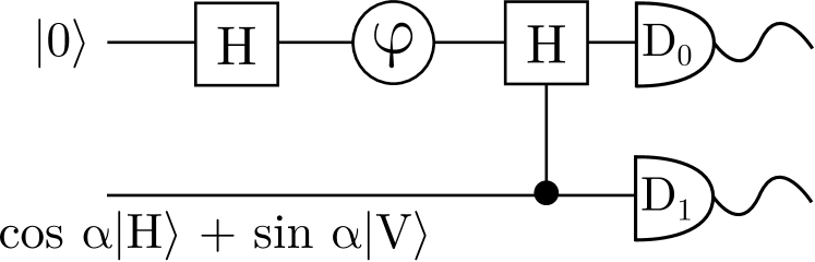
Conceptually, the quantum delayed-choice experiment [10] is conveniently represented by a quantum-gate network, see Fig.2. The first Hadamard operation, equivalent to the operation of beam splitter BS1, transforms the initial state into the superposition , where and represent the optical paths (spatial modes) of the photon in the MZI. The phase shifter changes the relative phase between the optical paths. This results in the spatial state of the photon. In the quantum delayed-choice experiment beam splitter BS2 is controlled by an ancilla and can be in a superposition of being present and absent. In the experimental realization [10] the polarization state of the photon is taken to be the ancilla. If the photon is horizontally polarized (), then the photon can pass BS2 (closed MZI) and if it is vertically polarized () then it cannot pass BS2 (open MZI). Hence, BS2 is a polarization controlled beam splitter.
If the ancilla is prepared in the state , where denotes the polarization angle of the photon, then the total state of the photon before arriving at BS2 reads . After the operation of the second Hadamard gate (BS2) this state becomes , where and describes wave-like behavior. The extra phase shifts and originate from the specific experimental set-up [10].
There are now two ways to proceed. First, considering the polarization states and in as a label for the particle and wave properties, a classical mixture of these properties is described by the mixed state . This corresponds to Wheeler’s delayed choice experiment [5, 20]. In this case the normalized intensities at detectors and are given by
| (1) |
and
| (2) |
respectively. Second, by measuring the ancilla in the basis the photon state becomes . This measurement can be performed by placing 45∘ polarizers in between BS2 and the detectors and . In this quantum delayed-choice experiment the non-normalized intensities at detectors and are given by [10]
| (3) |
and
| (4) |
respectively. The normalized intensities then read and , respectively.
3 Experimental realization
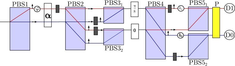
The diagram of the experimental set-up used by Tang et al. [10] is shown in Fig. 3. Except for the photon source it depicts all the optical components that are being used. The source, an InAs/GaAs self-assembled quantum dot [10], emits polarized single photons. The polarization state () of the photon is used as the ancilla and plays the role of the control qubit represented in Fig. 2 by the bottom line. The path of the photon corresponds to the target qubit, represented by the top line in Fig. 2.
The correspondence between the components of the quantum network Fig. 2 and the experimental realization depicted in Fig. 3 is as follows (throughout we adopt the quantum theoretical, wave mechanical picture). The first polarizing beam splitter PBS1 and the phase shifter perform the first Hadamard and phase shift operation. The half wave plate (HWP) with angle creates the superposition of both an open and a closed MZI, that is it prepares the ancilla in the state . The HWP behind the HWP with angle (and all other HWPs represented by the same graphic symbol) serves as a compensator: they have no equivalent in the quantum network Fig. 2 but they are essential to the physical realization of the experiment. Depending on the polarization state of the photon, PBS2 directs the photons (i.e. split the probability wave) in an upper pair and lower pair of paths. These two paths correspond to the two possible states of the target qubit in Fig. 2. The upper(bottom) pair of paths realizes the closed(open) MZI. Note that two lines within each pair correspond to the polarization state of the photon, i.e. they represent the two possible states of the ancilla in the quantum network. The controlled Hadamard gate in Fig. 2 is realized by the components PBS31, PBS32, the HWP’s at angles 0 and , PBS4, PBS51 and PBS52. The paths of the open and closed MZI merge at PBS5. Up to this point in the diagram in Fig. 3, the successive operations of the optical components on the photons implements the action of the quantum gates in Fig. 2 on a 2-qubit system.
In the work of Tang et al. [10], two cases are considered. In the first case, the polarizer P is in place (see Fig. 3) and points in the direction. A photon leaving the polarizer is counted by either detector or . In the second case, the polarizer P is absent and photons passing through PBS51 (PBS52) are counted at detector (). In our simulation work, we assume that the single-photon detectors have 100% detection efficiency, that is we count every photon that is emitted by the source.
4 Event-based simulation
The simulation model is a one-to-one copy of the quantum delayed-choice experiment [10]. A single photon is represented by a messenger that travels through the network [17, 22], the diagram of which is a copy of the experimental set-up and hence is the same as Fig. 3. The creation of a photon by the source corresponds to an event that creates a messenger. The message carried by the messenger consists of a two-dimensional, complex-valued unit vector [17, 22], representing the two electric field components which are orthogonal to the direction of propagation. It may help to think of the messenger as carrying a normalized Jones vector [2].
In the event-based approach, optical components are represented by processing units which accept a messenger, interpret and transform its messages and send out a messenger with its modified message [21, 17, 22]. The frequency distributions of detection events are generated event-by-event, meaning that at any time only a single messenger travels through the network of components whilst at any given time it has a definite position. Hence the single clicks that are produced by the detectors (which in our simulation are assumed to count every event that impinges on the detectors) build up the interference pattern one-by-one, exactly as in the laboratory experiment.
In the present work, the optical components are represented by exactly the same processing units as the ones used in earlier work [21, 17, 22]. For completeness, we briefly describe the action of each processing unit that appears in Fig. 3. The Python code listed in the Appendix provides the complete specification the algorithm that we have used to produce the data reported in the present paper.
Polarizing beam splitter (PBS): This optical component is represented by a two-input – two-output processor. A messenger arriving at one of its input ports causes the internal state (represented by ten floating-point numbers) of the processor to be updated. The update rule consists of storing the message into memory local to the processor and changing a two-dimensional vector, also local to the processor, which serves to estimate the relative number of messengers arriving at the two different input ports.
Pictorially, the update rule mimics the change of the polarization of the dielectric due to the interaction of the latter with electric field [19]. The ten numbers contained in the internal state are used to build a unit vector which is then multiplied by the unitary transformation which is the same as the one used in the classical (and quantum) wave mechanical description of a polarizing beam splitter [25, 26]. The resulting unit vector is then used to (i) decide at which output port the messenger will leave the unit and (ii) to construct the new message which the messenger will carry. The technical details of examples of the implementation of the algorithm that we have just described are given in Refs. [21, 17, 22]. It is important to note that the processing unit does not store information from all the messengers that it processes: it only has a very limited amount of memory, namely ten floating point numbers only.
Since both the memory of the processing unit and a (pseudo) random number is taken into account to generate an output message, there is no one-to-one relation between the input and the output message. Hence, this processing unit is indeed different from, and therefore there is also no correspondence with, the unitary time evolution of quantum theory. Unlike the suggestion made in Fig. 3, in the event-based simulation both PBS2 and PBS4 are represented by two identical but logically independent processing units.
Phase shifters: In the event-based approach, phase shifters change the time of flight of the messenger, corresponding to a rotation of the unit vector encoding the message by e.g. , or .
Polarizer: The polarizer is modeled as a PBS which is rotated about 45 degrees, corresponding to the change of the basis from to , and by destroying all messengers which leave the PBS via one of the output ports and keeping all others.
Half wave plate (HWP): a HWP is modeled as a passive device that rotates the message according to the unitary matrix which is characterized by , the angle between the optical axis and the laboratory frame [17, 2].
Looking at Fig. 3, the solid rectangles represent HWPs with whilst the other HWPs have angles as indicated.
Detectors: In our simulations, the detectors are considered to be ideal. This means that whenever a messenger reaches the detector, the detector count is incremented by one.
5 Simulation procedure
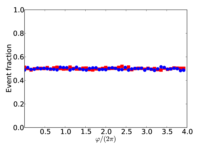
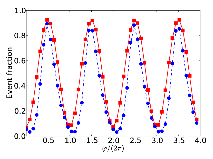
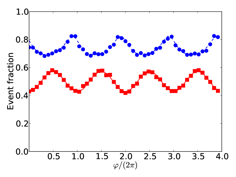
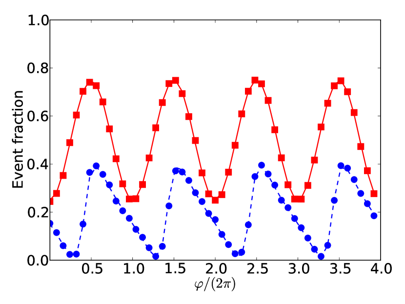
As in the experiment [10], we perform two sets of simulations: One with and one without the polarizer in front of the detectors (see Fig. 3). For the angle of polarization we take for , the values for which Ref. [10] reports experimental data. As Ref. [10] does not mention the values of the phase shifts and , we adjust these parameters such that the quantum theoretical and event-based simulation results look very similar to the experimental data. The results presented here have been obtained by taking and . Note that quantum theory predicts that the choice of these two parameters only affects the results if the polarizer P is present (compare Eqs. (1,2) and Eqs. (3,4)).
For each set of values of the phase shift and rotation angle , the internal states of the processing units are initialized by means of different pseudo-random numbers. The data collection consists of sending, one-by-one, messengers through the network. Only after a messenger has been processed by a detector unit or has been destroyed by the polarizer P, a new messenger is being created. At creation, the messenger carries as message the unit vector corresponding to a linear polarization of 45 degrees.
Every messenger that arrives at a detector increases the corresponding event count by one. The relative detection count is obtained by dividing the event count by the total number of events registered by both detectors.
6 Simulation results
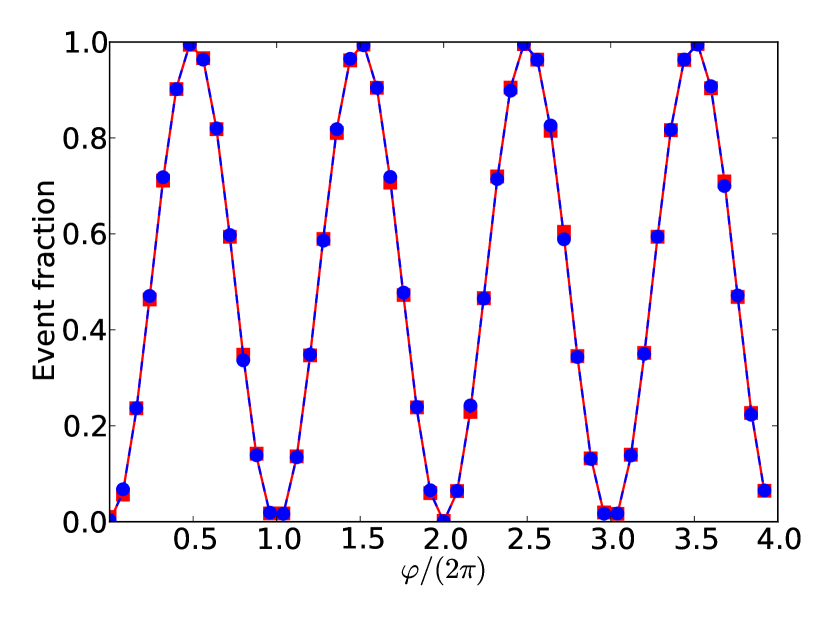
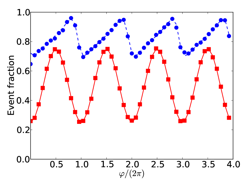
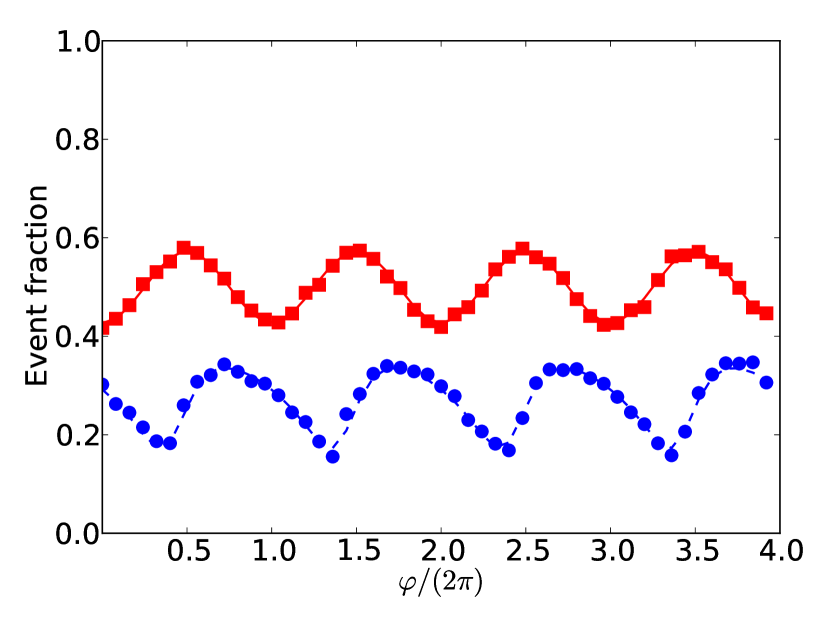
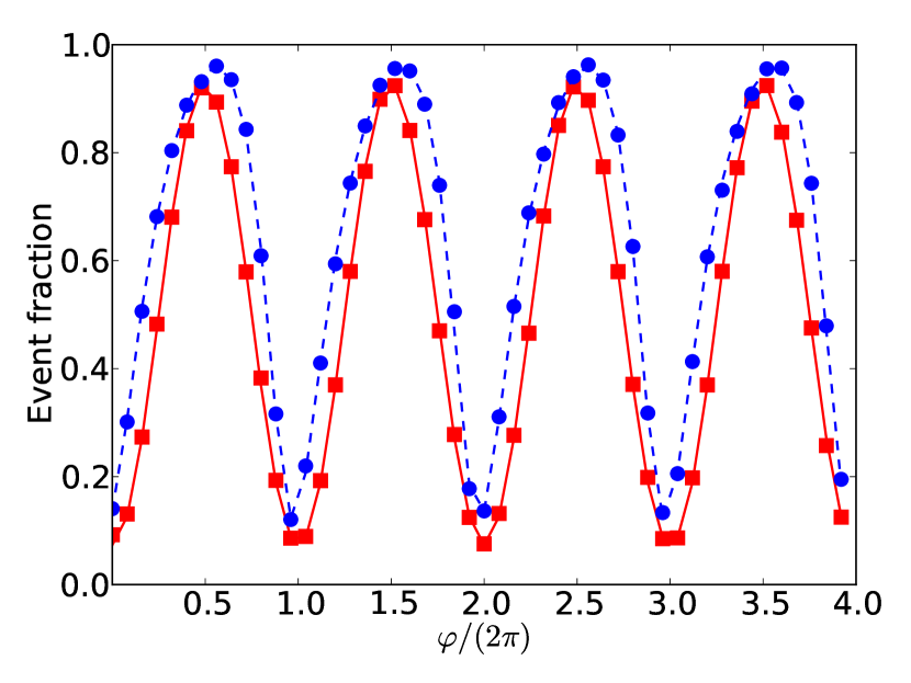
The simulation procedure outlined above is repeated for 50 different values of the phase shift , yielding the plots presented in Fig. 4. The fraction of events arriving at is plotted as a function of the phase difference . The (red) squares represent the event-based simulation data for the set-up without the polarizer P and the (red) solid lines are the corresponding quantum theoretical predictions (see Eq. (2)). The (blue) circles represent the event-based simulation results for the set-up with the polarizer P present and the (blue) dashed lines are the predictions according to quantum theory (Eq. (4)). Each subpanel shows the results for a different value of . In all cases there is excellent agreement between the simulation data and the quantum theoretical description. Therefore, we have established that the “morphing” of the particle and wave nature of the photon in a quantum delayed-choice experiment [10] can be explained without recourse to concepts of quantum theory.
7 Discussion
As mentioned in the introduction, the event-based approach has successfully been applied to a large variety of single-photon and single-neutron experiments that involve interference and entanglement. In the present paper, we have shown that, without any modification, the same simulation approach can also mimic, event-by-event, a quantum delayed choice experiment. As none of these demonstrations rely on concepts of quantum theory and as it is unlikely that the success of all these demonstrations is accidental, one may wonder what it is that makes a system genuine “quantum”. Indeed, if a physicist living before the era of quantum physics was asked to calculate the intensities for the set-up depicted in Fig. 3 he would have had no problems finding the correct expressions using classical electrodynamics. What makes this experiment quantum (as opposed to classical) is the fact that single indivisible entities called photons traverse the apparatus, one single quantum at a time. Yet, paradoxically this is precisely what quantum theory cannot describe since it can only describe the statistical distribution, not the single events. The event-by-event approach fills in this gap by combining classical electrodynamics with the notion of particles (which is not part of Maxwell’s theory). The key to produce interference patterns without having to rely on a wave equation is the introduction of an adaptive processing element which simulates the interaction between single particles and the optical components, akin to the classical electrodynamics description of the response of the polarization of the material to the applied electric field. There are several different ways to implement such adaptive processing elements and although the details of their dynamics is different, in the stationary state they yield the same frequency distributions for observing the events [15, 17]. In order to determine which of these implementations is closer to what actually happens in experiments (on the level of individual events), it is necessary to perform new experiments which specifically address this question.
To further address the question what makes a certain system genuine “quantum” it is of interest to recall Bohr’s point of view that “There is no quantum world. There is only an abstract physical description” (reported by [27], for a discussion see [28]) and that “The physical content of quantum mechanics is exhausted by its power to formulate statistical laws” [29]. Or, to say it differently “Quantum theory describes our knowledge of the atomic phenomena rather than the atomic phenomena themselves” [30]. In other words, quantum theory captures, and does so extremely well, the inferences that we, humans, make on the basis of experimental data [31]. However it does not describe cause-and-effect processes. Quantum theory predicts the probabilities that events occur, but it cannot answer the question “Why are there events?” [13]. The logical contradictions, often referred to as mysteries [24], created by the (quantum) delayed choice experiment are a direct consequence of trying to explain the existence of events within the realm of quantum theory proper. The point of view that we take in developing event-based descriptions is that on a basic level, it is our perceptual and cognitive system that defines, registers and processes events. Therefore, events themselves and the rules that create new events are taken to be the key elements in the construction of the event-based models.
In conclusion, the implication of the work presented in the present paper is that the results of the beautiful quantum-delayed choice experiment of Tang et al. [10] can be explained entirely in terms of cause-and-effect, discrete-event processes, without making reference to quantum or wave theory and invoking concepts and ideas that defy common sense [24]. In particular, it is not necessary to introduce the idea of morphing between the particle- and wave-like behavior of photons [6], a particle-only description suffices to account for the experimental observations.
8 Acknowledgement
K.M. would like to thank Pablo Manuel Cencillo Abad for exploratory research work.
Appendix: Python program
The program listed below generates the figures presented in Fig. 4, up to small fluctuations that are due to the use of pseudo-random numbers. The program has been tested with Python version 2.7.2 (Windows 7) and Python 2.7.6 (Linux 3.13.0-24), with matplotlib installed. Depending on the CPU used, it may take considerable time (an hour or more) to produce all 8 figures. To check if the program runs it may be convenient to change num_data_points = 50 and num_iter = 10000 into num_data_points = 10 and num_iter = 1000, respectively. Progress of the calculation is indicated on the screen.
References
References
- [1] P. Grangier, G. Roger, A. Aspect, Experimental evidence for a photon anticorrelation effect on a beam splitter: A new light on single-photon interferences, Europhys. Lett. 1 (1986) 173 – 179.
- [2] F. Pedrotti, L. Pedrotti, L. Pedrotti, Introduction to Optics, Pearson Education, London, 2007.
- [3] J. Baldzun, E. Molher, W. Martienssen, A wave-particle delayed-choice experiment with a single-photon state, Z. Phys. B 77 (1989) 347 – 352.
- [4] T. Hellmuth, H. Walther, A. Zajonc, W. Schleich, Delayed-choice experiments in quantum interference, Phys. Rev. A 72 (1987) 2532 – 2541.
- [5] V. Jacques, E. Wu, F. Grosshans, F. Treussart, P. Grangier, A. Aspect, J.-F. Roch, Experimental realization of Wheeler’s delayed-choice gedanken experiment, Science 315 (2007) 966 – 968.
- [6] R. Ionicioiu, D. R. Terno, Proposal for a quantum delayed-choice experiment, Phys. Rev. Lett. 107 (2011) 230406.
- [7] S. S. Roy, A. Shukla, T. S. Mahesh, NMR implementation of a quantum delayed-choice experiment, Phys. Rev. A 85 (2012) 022109.
- [8] R. Auccaise, R. M. Serra, J. G. Filgueiras, R. S. Sarthour, I. S. Oliveira, L. C. Celeri, Experimental analysis of the quantum complementarity principle, Phys. Rev. A 85 (2012) 032121.
- [9] A. Peruzzo, P. Shadbolt, N. Brunner, S. Popescu, J. L. O’Brien, A quantum delayed-choice experiment, Science 338 (6107) (2012) 634 – 637.
- [10] J.-S. Tang, Y.-L. Li, X.-Y. Xu, G.-Y. Xiang, C.-F. Li, G.-C. Guo, Realization of quantum Wheeler’s delayed-choice experiment, Nat. Photonics 6 (2012) 600 – 604.
- [11] F. Kaiser, T. Coudreau, P. Milman, D. B. Ostrowsky, S. Tanzilli, Entanglement-enabled delayed-choice experiment, Science 338 (6107) (2012) 637 – 640.
- [12] A. J. Leggett, Quantum mechanics at the macroscopic level, in: J. de Boer, E. Dal, O. Ulfbeck (Eds.), The Lessons of Quantum Theory: Niels Bohr Centenary Symposium, Elsevier, Amsterdam, 1987, pp. 35 – 58.
- [13] B-G. Englert, On quantum theory, Eur. Phys. J. D 67 (2013) 238.
- [14] J. Wheeler, Information, physics, quantum: The search for links, in: 3rd Int. Symp. Foundations of Quantum Mechanics, 1989, pp. 354 – 368.
- [15] H. De Raedt, K. De Raedt, K. Michielsen, Event-based simulation of single-photon beam splitters and Mach-Zehnder interferometers, Europhys. Lett. 69 (2005) 861 – 867.
- [16] K. De Raedt, H. De Raedt, K. Michielsen, Deterministic event-based simulation of quantum interference, Comp. Phys. Comm. 171 (2005) 19 – 39.
- [17] K. Michielsen, F. Jin, H. De Raedt, Event-based corpuscular model for quantum optics experiments, J. Comput. Theor. Nanosci. 8 (2011) 1052 – 1080.
- [18] H. De Raedt, K. Michielsen, Event-by-event simulation of quantum phenomena, Ann. Phys. (Berlin) 524 (2012) 393 – 410.
- [19] H. De Raedt, F. Jin, K. Michielsen, Event-based simulation of neutron interferometry experiments, Quantum Matter 1 (2012) 1 – 21.
- [20] V. Jacques, E. Wu, F. Grosshans, F. Treussart, P. Grangier, A. Aspect, J.-F. Roch, Delayed-choice test of quantum complementarity with interfering single photons, Phys. Rev. Lett. 100 (2008) 220402.
- [21] S. Zhao, S. Yuan, H. De Raedt, K. Michielsen, Computer simulation of Wheeler’s delayed choice experiment with photons, Europhys. Lett. 82 (2008) 40004.
- [22] H. De Raedt, M. Delina, F. Jin, K. Michielsen, Corpuscular event-by-event simulation of quantum optics experiments: application to a quantum-controlled delayed-choice experiment, Phys. Scr. T151 (2012) 014004.
- [23] K. Michielsen, K. De Raedt, H. De Raedt, Simulation of quantum computation: a deterministic event-based approach, J. Comput. Theor. Nanosci. 2 (2005) 227 – 239.
- [24] A. Ananthaswamy, Quantum shadows: The mystery of matters deepens, New Scientist 2898 (2013) 36 – 39.
- [25] J. C. Garrison, R. Y. Chiao, Quantum Optics, Oxford University Press, Oxford, 2008.
- [26] H. Bachor, T. Ralph, A Guide to Experiments in Quantum Optics, Wiley-VCH Verlag, Weinheim, 2008.
- [27] A. Petersen, The philosophy of Niels Bohr, Bulletin of the Atomic Scientists 19 (1963) 8 – 14.
- [28] A. Plotnitsky, ”Epistemology and Probability: Bohr, Heisenberg, Schrödinger, and the Nature of Quantum-Theoretical Thinking”, Springer, Berlin, 2010.
- [29] N. Bohr, XV. The Unity of Human Knowledge, in: D. Favrholdt (Ed.), Complementarity Beyond Physics (1928 –1962), Vol. 10 of Niels Bohr Collected Works, Elsevier, Amsterdam, 1999, pp. 155 – 160.
- [30] K. V. Laurikainen, The Message of the Atoms. Essays on Wolfgang Pauli and the Unspeakable, Springer, Berlin, 1997.
- [31] H. De Raedt, M. Katsnelson, K. Michielsen, Quantum theory as the most robust description of reproducible experiments, Ann. Phys. 347 (2014) 45 – 73.