A Preconditioned Hybrid SVD Method for Computing Accurately Singular Triplets of Large Matrices

Abstract

The computation of a few singular triplets of large, sparse matrices is a challenging task, especially when the smallest magnitude singular values are needed in high accuracy. Most recent efforts try to address this problem through variations of the Lanczos bidiagonalization method, but they are still challenged even for medium matrix sizes due to the difficulty of the problem. We propose a novel SVD approach that can take advantage of preconditioning and of any well designed eigensolver to compute both largest and smallest singular triplets. Accuracy and efficiency is achieved through a hybrid, two-stage meta-method, PHSVDS. In the first stage, PHSVDS solves the normal equations up to the best achievable accuracy. If further accuracy is required, the method switches automatically to an eigenvalue problem with the augmented matrix. Thus it combines the advantages of the two stages, faster convergence and accuracy, respectively. For the augmented matrix, solving the interior eigenvalue is facilitated by a proper use of the good initial guesses from the first stage and an efficient implementation of the refined projection method. We also discuss how to precondition PHSVDS and to cope with some issues that arise. Numerical experiments illustrate the efficiency and robustness of the method.

1 Introduction

The Singular Value Decomposition (SVD) is a ubiquitous computational kernel in science and engineering. Many, highly diverse applications require a few of the largest singular values of a large sparse matrix $A$ and the associated left and right singular vectors (singular triplets). These triplets play a critical role in compression and model reduction. A smaller, but increasingly important, set of applications requires a few smallest singular triplets. Examples include least squares problems, determination of matrix rank, low rank approximation, and computation of pseudospectrum [13, 37]. Recently we have used such techniques to reduce the variance in Monte Carlo estimations of the the trace of the inverse of a large sparse matrix.

It is well known that the computation of the smallest singular triplets presents challenges both to the speed of convergence and the accuracy of iterative methods. In this paper, we mainly focus on the problem of finding the smallest singular triplets. Assume $A\in\Re^{m\times n}$ is a large sparse matrix with full column rank and $m\geq n$. The (economy size) singular value decomposition of A can be written as:

(1) $$A=U\Sigma V^{T}$$

where $U=[u_{1},\ldots,u_{n}]\in\Re^{m\times n}$ is an orthonormal set of the left singular vectors and $V=[v_{1},\ldots,v_{n}]\in\Re^{n\times n}$ is the unitary matrix of the right singular vectors. $\Sigma=diag(\sigma_{1},\ldots,\sigma_{n})\in\Re^{n\times n}$ contains the singular values of $A$, $\sigma_{1}\leq\ldots\leq\sigma_{n}$. We will be looking for the smallest $k\ll n$ singular triplets $\{\sigma_{i},u_{i},v_{i}\},i=1,\ldots,k$.

There are two approaches to compute the singular triplets $\{\sigma_{i},u_{i},v_{i}\}$ by using a Hermitian eigensolver. Using MATLAB notation, the first approach seeks eigenpairs of the augmented matrix $B=[0\ A^{T};A\ 0]\in\Re^{(m+n)\times(m+n)}$, which has eigenvalues $\pm\sigma_{i}$ with corresponding eigenvectors $([v_{i};u_{i}],[-v_{i};u_{i}])$, as well as $m-n$ zero eigenvalues [11, 12, 8]. The main advantage of this approach is that iterative methods can potentially compute the smallest singular values accurately, i.e., with residual norm close to $O(\|A\|\epsilon_{mach})$. However, convergence of eigenvalue iterative methods is slow since it is a highly interior eigenvalue problem, and even the use of iterative refinement or inverse iteration involves a maximally indefinite matrix [28]. For restarted iterative methods convergence is even slower, irregular, and often the required eigenvalues are missed since the Rayleigh-Ritz projection method does not effectively extract the appropriate information for interior eigenvectors [25, 26, 17].

The second approach computes eigenpairs of the normal equations matrix $C=A^{T}A\in\Re^{n\times n}$ which has eigenvalues $\sigma_{i}^{2}$ and associated eigenvectors $v_{i}$. If $\sigma_{i}\neq 0$, the corresponding left singular vectors are obtained as $u_{i}=\frac{1}{\sigma_{i}}A^{T}v_{i}$. $C$ is implicitly accessed through successive matrix-vector multiplications. The squaring of the singular values works in favor of this approach with Krylov methods, especially with largest singular values since their relative separations increase. Although the separations of the smallest singular values become smaller, we show in this paper that this approach still is faster than Krylov methods on $B$ because it avoids indefiniteness. On the other hand, squaring the matrix limits the accuracy at which smallest singular triplets can be obtained. Therefore, this approach is typically followed by a second stage of iterative refinement for each needed singular triplet [29, 10, 7]. However, this one-by-one refinement does not exploit information from other singular vectors and thus is it not as efficient as an eigensolver applied on $B$ with the estimates of the first stage.

The Lanczos bidiagonalization (LBD) method [13, 11] is accepted as an accurate and more efficient method for seeking singular triplets (especially smallest), and numerous variants have been proposed [22, 18, 20, 2, 3, 4, 19]. LBD builds the same subspace as Lanczos on matrix $C$, but since it works on $A$ directly, it avoids the numerical problems of squaring. However, the Ritz vectors often exhibit slow, irregular convergence when the smallest singular values are clustered. To address this problem, harmonic projection [20, 2], refined projection [18], and their combinations [19] have been applied to LBD. Despite remarkable algorithmic progress, current LBD methods are still in development, with only few existing MATLAB implementations that serve mainly as a testbed for mathematical research. We show that a two stage approach based on a well designed eigenvalue code can be more robust and efficient for a few singular triplets. Most importantly, our approach can use preconditioning through the eigensolver, which is not directly possible with LBD but becomes crucial because of the difficulty of the problem even for medium matrix sizes.

The Jacobi-Davidson type SVD method, JDSVD [15, 16], is based on an inner-outer iteration and can also use preconditioning. It obtains the left and right singular vectors directly from a projection of $B$ on two subspaces and, although it avoids the numerical limitations of matrix $C$, it needs a harmonic [25, 27, 32] or a refined projection method [17, 36] to avoid irregular Rayleigh-Ritz convergence. JDSVD often has difficulty computing the smallest singular values of a rectangular matrix, especially without preconditioning, due to the presence of zero eigenvalues of $B$.

SVDIFP is a recent extension to the inverse free preconditioned Krylov subspace method, [14], for the singular value problem [24]. The implementation includes the robust incomplete factorization (RIF) [6] for the normal equations matrix, but other preconditioners can also be used. To circumvent the intrinsic difficulties of filtering out the zero eigenvalues of $B$, the method works with the normal equations matrix $C$, but computes directly the smallest singular values of $A$ and not the eigenvalues of $C$. Thus good numerical accuracy can be achieved but, as we show later, at the expense of efficiency. Moreover, the design of SVDIFP is based on restarting with a single vector, which is not effective when seeking more than one singular values.

In this paper we present a preconditioned hybrid two-stage method, PHSVDS, that achieves both efficiency and accuracy for both largest and smallest singular values under limited memory. In the first stage, the proposed method PHSVDS solves an extreme eigenvalue problem on $C$ up to the user required accuracy or up to the accuracy achievable by the normal equations. If further accuracy is required, PHSVDS switches to a second stage where it utilizes the eigenvectors and eigenvalues from $C$ as initial guesses to a Jacobi-Davidson method on $B$, which has been enhanced by a refined projection method. The appropriate choices for tolerances, transitions, selection of target shifts, and initial guesses are handled automatically by the method. We also discuss how to precondition PHSVDS and to cope with possible issues that can arise. Our extensive numerical experiments show that PHSVDS, implemented on top of the eigensolver PRIMME [34], can be considerably more efficient than all other methods when computing a few of the smallest singular triplets, even without a preconditioner. With a good preconditioner, the PHSVDS method can be much more efficient and robust than the JDSVD and SVDIFP methods.

In Section 2 we motivate the two stage SVD method based on the convergence of Krylov methods to the smallest magnitude eigenvalue of $B$ and $C$. In Section 3, we develop the components of the two stage method. In Section 4, we describe how to precondition PHSVDS, and how to dynamically inspect the quality of preconditioning at the two different stages. In Section 5, we present extensive experiments that corroborate our conclusions.

We denote by $\|.\|$ the 2-norm of a vector or a matrix, by $A^{T}$ the transpose of $A$, by $I$ the identity matrix, $\kappa(A)=\frac{\sigma_{n}}{\sigma_{1}}$, and by $K_{k}(A,v)=span\{v,Av,\ldots,A^{k-1}v\}$ the k-dimensional Krylov subspace generated by $A$ and the initial vector $v$.

2 Motivation for a two stage strategy

We first need to understand whether an eigensolver on $C$ or on $B$ is preferable in terms of convergence and accuracy to iterative solvers that solve the SVD directly. To address this, we introduce the basic SVD iterative methods and study the asymptotic convergence and the quality of the Krylov subspaces built by different methods. We conclude that an appropriate choice of eigensolvers and eigenvalue problem yields methods that are faster and equally accurate as the best SVD methods, especially in the presence of limited memory.

2.1 The LBD, JDSVD, and SVDIFP methods

The LBD method, [11, 12], starts with unit vectors $p_{1}$ and $q_{1}$ and after $k$ steps produces the following decomposition as a partial Lanczos bidiagonalization of $A$:

(2) $$AP_{k}=Q_{k}B_{k},$$

$$A^{T}Q_{k}=P_{k}B_{k}^{T}+r_{k}e_{k}^{T},$$

where the $r_{k}$ is the residual vector at $k$-th step, $e_{k}$ the $k-$th orthocanonical vector,

$$B_{k}=\left(\begin{array}[]{cccc}\alpha_{1}&\beta_{1}&&\\ &\alpha_{2}&\ddots&\\ &&\ddots&\beta_{k-1}\\ &&&\alpha_{k}\end{array}\right)=Q_{k}^{T}AP_{k},$$

and $Q_{k}$ and $P_{k}$ are orthonormal bases of the Krylov subspaces $K_{k}(AA^{T},q_{1})$, and $K_{k}(A^{T}A,p_{1})$ respectively. With properly chosen starting vectors, LBD produces mathematically the same space as the symmetric Lanczos method on $B$ or $C$ [19, 20].

To approximate singular triplets of $A$, LBD solves the small singular value problem on $B_{k}$, and uses the corresponding Ritz approximations from $Q_{k}$ and $P_{k}$ as left and right singular vectors. To address the rapid loss of orthogonality of the columns of $Q_{k}$ and $P_{k}$ in finite precision arithmetic, full [12], partial [22], or one-sided reorthogonalization [2, 19] strategies have been applied to variants of LBD. With appropriate implementation, these can result in a backward stable algorithm for both singular values and vectors [5, 19]. Because, all these solutions become expensive when $k$ is large, restarted LBD versions have been studied [20, 2, 18, 22]. The goal is twofold: restart with sufficient subspace information to maintain a good convergence, and identify the appropriate Ritz information to restart with. The former problem is tackled with implicit or thick restarting [35]. The latter problem is tackled with combinations of harmonic and refined projection methods. For example, IRLBA [3] uses a thick restarted block LBD with harmonic projection, while IRRHLB [19] first computes harmonic Ritz vectors, and then uses their Rayleigh quotients in a refined projection to extract refined Ritz vectors from $P_{k}$ and $Q_{k}$.

The JDSVD method [15] extends the Jacobi-Davidson method and its correction equation for singular value problems by exploiting the special structure of the augmented matrix $B$. Similarly to LBD, JDSVD computes singular values, not eigenvalues, of the projection matrix, and the left and right singular vectors from separate spaces. Because good quality approximations are important not only for restarting but also in the correction equation, various projection methods can benefit JDSVD. We introduce only the standard choice where the test and search space are the same.

Let $U$ and $V$ be the bases of the left and right search spaces. Computing a singular triplet $(\theta,c,d)$ of $H=U^{T}AV$ yields $(\theta,Uc,Vd)$ as the Ritz approximation of a corresponding singular triplet of $A$. Alternatively, the $u=Uc$ and $v=Vc$ can be computed as harmonic or refined singular triplets. Then JDSVD obtains corrections $s$ and $t$ for $u$ and $v$ by solving (approximately) the following correction equation:

(3) $$\left(\begin{array}[]{cc}P_{u}&0\\ 0&P_{v}\end{array}\right)\left(\begin{array}[]{cc}-\theta I_{m}&A\\ A^{T}&-\theta I_{n}\end{array}\right)\left(\begin{array}[]{cc}P_{u}&0\\ 0&P_{v}\end{array}\right)\left(\begin{array}[]{c}s\\ t\end{array}\right)=\left(\begin{array}[]{c}Av-\theta u\\ A^{T}u-\theta v\end{array}\right)$$

where $P_{v}=I_{n}-vv^{T},P_{u}=I_{m}-uu^{T}$. The left and right corrections $s,t$ are then orthogonalized against and appended to $U$ and $V$ respectively. JDSVD uses thick restarting [35, 38] but retains also Ritz vectors from the previous iteration, similarly to the locally optimal Conjugate Gradient recurrence [33]. Most importantly, the JDSVD method can take advantage of preconditioning when solving (3).

The SVDIFP method [24] extends the EIGIFP method [14]. Given an approximation $(x_{i},\rho_{i})$ at the $i$-th step of the outer method, it builds a Krylov space ${\cal V}=K_{k}(M(C-\rho_{i}I),x_{i})$, where $M$ is a preconditioner for $C$. To avoid the numerical problems of projecting on $C$, SVDIFP computes the smallest singular values of $A{\cal V}$, by using a two sided projection similarly to the LBD. Because the method focuses only the right singular vector, the left singular vectors can be quite inaccurate.

2.2 Asymptotic convergence of Krylov methods on $C$ and $B$

When seeking largest singular values, it is accepted that Krylov methods on $C$ are faster than on $B$ [15, 20, 24, 7]. The argument is straightforward.

Theorem 1.

Let $\gamma_{B}=\frac{\sigma_{n}-\sigma_{n-1}}{\sigma_{n-1}+\sigma_{n}}$ and $\gamma_{C}=\frac{\sigma_{n}^{2}-\sigma_{n-1}^{2}}{\sigma_{n-1}^{2}-\sigma_{1}^{2}}$ be the gap ratios of the largest eigenvalue of matrices $B$ and $C$, respectively. Then, for the largest eigenvalue, the asymptotic convergence of Lanczos on $C$ is $2$ times faster than Lanczos on $B$.

Proof.

The asymptotic convergence rate is the square root of the gap ratio. Then:

$$\gamma_{C}=\frac{(\sigma_{n}-\sigma_{n-1})(\sigma_{n}+\sigma_{n-1})^{2}}{(\sigma_{n}+\sigma_{n-1})(\sigma_{n-1}^{2}-\sigma_{1}^{2})}=\gamma_{B}\frac{(\sigma_{n}+\sigma_{n-1})^{2}}{(\sigma_{n-1}^{2}-\sigma_{1}^{2})}>\gamma_{B}\frac{4\sigma_{n-1}^{2}}{(\sigma_{n-1}^{2}-\sigma_{1}^{2})}=\frac{4\gamma_{B}}{1-(\frac{\sigma_{1}}{\sigma_{n-1}})^{2}}.$$

Therefore, for $\sigma_{1}\approx 0$, the asymptotic convergence rate $\sqrt{\gamma_{C}}>2\sqrt{\gamma_{B}}$. In the less interesting case $\sigma_{1}\rightarrow\sigma_{n-1}$, Lanczos on $C$ is arbitrarily faster than on $B$. ∎

For smallest singular values the literature is less clear, although methods that work on $C$ have been avoided for numerical reasons. In previous experiments we have observed much faster convergence with approaches on $C$ than on $B$ [39]. To obtain some intuition, we perform a basic asymptotic convergence analysis of Krylov methods working on $C$ or on $B$ trying to compute the smallest magnitude eigenvalue.

Lemma 2.

Let the union of two intervals: $K=[-a,-b]\cup[c,d]$, $-b<0<c$, and $p_{k}(x)$ the optimal degree $k$ polynomial that is as small as possible on $K$ and $p_{k}(0)=1$. Let $\epsilon_{k}=\max_{x\in K}|p_{k}(x)|$, and $\rho=\lim_{k\rightarrow\infty}\epsilon_{k}^{1/k}$. Then asymptotically:

$$\rho\simeq 1-\sqrt{\frac{bc}{da}}.$$

Proof.

This is an application of Theorem 5 in [31]. ∎

This $\rho$ translates to an upper bound for the asymptotic convergence rate of any Krylov solver applied to an indefinite matrix whose spectrum lies in the interval $K$. Thus it can also be used for the convergence rate to the smallest positive eigenvalue of the augmented matrix $B$. Assume $\sigma_{1}$ is a simple eigenvalue of $B$ and thus $\sigma_{1}^{2}$ is a simple eigenvalue of $C$. Define its gap ratio in $C$ as, $\gamma=\frac{\sigma_{2}^{2}-\sigma_{1}^{2}}{\sigma_{n}^{2}-\sigma_{2}^{2}}$, and assume $\gamma\ll 1$.

Theorem 3.

Consider the spectrum of the matrix $B-\sigma_{1}I$, which lies (except for the zero eigenvalue) in the two intervals: $K=[-\sigma_{n}-\sigma_{1},-2\sigma_{1}]\cup[\sigma_{2}-\sigma_{1},\sigma_{n}-\sigma_{1}]$. The asymptotic convergence rate for any Krylov solver that finds $\sigma_{1}$ is bounded by:

$$\rho=1-\sqrt{\gamma\ \frac{2\sigma_{1}}{\sigma_{2}+\sigma_{1}}\ \frac{\sigma_{n}^{2}-\sigma_{2}^{2}}{\sigma_{n}^{2}-\sigma_{1}^{2}}}.$$

Proof.

Clearly, the optimal polynomial $p_{k}(x)$ of Lemma 2 is the best polynomial for finding $\sigma_{1}$. Applying the Lemma for the specific bounds for this interval we get:

$$\frac{bc}{ad}=\frac{2\sigma_{1}(\sigma_{2}-\sigma_{1})}{(\sigma_{n}+\sigma_{1})(\sigma_{n}-\sigma_{1})}=\frac{2\sigma_{1}}{\sigma_{2}+\sigma_{1}}\ \frac{\sigma_{2}^{2}-\sigma_{1}^{2}}{\sigma_{n}^{2}-\sigma_{1}^{2}}=\frac{2\sigma_{1}}{\sigma_{2}+\sigma_{1}}\ \frac{\sigma_{2}^{2}-\sigma_{1}^{2}}{\sigma_{n}^{2}-\sigma_{2}^{2}}\ \frac{\sigma_{n}^{2}-\sigma_{2}^{2}}{\sigma_{n}^{2}-\sigma_{1}^{2}}.$$

∎

Lemma 4.

The bound of the asymptotic convergence rate to $\sigma_{1}^{2}$ of Lanczos on $C$ is approximately: $q=1-2\sqrt{\gamma}$.

Proof.

The bound on the rate of convergence of Lanczos for $\sigma_{1}^{2}$ is approximated as $e^{-2\sqrt{\gamma}}$ [28, p. 280]. Taking the first order approximation from Taylor series around 0, we obtain $e^{-2\sqrt{\gamma}}=1-2\sqrt{\gamma}+O(\gamma)$. ∎

Theorem 5.

A Krylov method on $C$ that computes $\sigma_{1}^{2}$ has always faster asymptotic convergence rate than a Krylov method on $B$ that finds $\sigma_{1}$, by a factor of

(4) $$\tau=\frac{1-\sqrt{\gamma}\sqrt{\frac{2\sigma_{1}}{\sigma_{2}+\sigma_{1}}\ \frac{\sigma_{n}^{2}-\sigma_{2}^{2}}{\sigma_{n}^{2}-\sigma_{1}^{2}}}}{1-2\sqrt{\gamma}}.$$

Proof.

For the method on $C$ to be faster it must hold $\tau>1$ or $\frac{2\sigma_{1}}{\sigma_{2}+\sigma_{1}}\ \frac{\sigma_{n}^{2}-\sigma_{2}^{2}}{\sigma_{n}^{2}-\sigma_{1}^{2}}<4$. Basic manipulations lead to the condition $(4-2\frac{\sigma_{n}^{2}-\sigma_{2}^{2}}{\sigma_{n}^{2}-\sigma_{1}^{2}})\sigma_{1}>=-4\sigma_{2}$. Since $\frac{\sigma_{n}^{2}-\sigma_{2}^{2}}{\sigma_{n}^{2}-\sigma_{1}^{2}}<1$ and all $\sigma_{i}>0$, the above condition always holds. ∎

First, we observe that if $\sigma_{1}$ is very close to 0, the normal equations approach becomes arbitrarily faster than the augmented one, as long as $\sigma_{2}$ remains bounded away from 0. Second, it is not hard to see that $\tau=1+O(\sqrt{\sigma_{2}-\sigma_{1}})$, which means that the two approaches become similar with highly clustered eigenvalues. In that case, however, using a block method would increase the gap ratios and the gains from the approach on $C$ would be larger again.

Most importantly, the above asymptotic convergence rates reflect optimal methods applied to $C$ and $B$ and an extraction of the best information from the subspaces. In practice, memory and computational requirements necessitate the restarting of iterative methods, which results in significant convergence slow down. For extremal eigenvalues, combinations of thick restarting with the locally optimal conjugate gradient directions have been shown to almost fully restore the convergence of the unrestarted Lanczos method. The GD+k and extensions to LOBPCG are such nearly-optimal methods [35, 33]. For interior eigenvalues, practical Krylov methods not only have a hard time achieving this convergence, but also have problems extracting the best eigenvectors from the subspace. Therefore, we expect in practice the normal equations to be significantly faster than any approach based on $B$.

2.3 Comparison of subspaces from Lanczos, LBD and JDSVD

We extend the discussion on Lanczos to include two native SVD methods, and infer the relative differences between their convergence by studying the subspace they build. A higher dimensional Krylov subspace implies faster convergence, assuming eigenvector approximations can be extracted effectively from the subspace. We compare LBD, JDSVD, and Lanczos (or equivalently unpreconditioned GD) on $C$ and on $B$.

Suppose $u_{1},v_{1}$ are left and right initial guesses. After $k$ iterations ($2k$ matvecs), Lanczos working on the normal equations matrix $C$ builds:

(5) $$V_{k}=K_{k}(A^{T}A,v_{1}).$$

The LBD method builds both left and right Krylov spaces [2]:

(6) $$U_{k}=K_{k}(AA^{T},Av_{1}),\qquad V_{k}=K_{k}(A^{T}A,v_{1}).$$

The JDSVD method also builds two subspaces, each being a direct sum of two Krylov spaces of half the dimension [15]:

(7) $$U_{k}=K_{\frac{k}{2}}(AA^{T},u_{1})\oplus K_{\frac{k}{2}}(AA^{T},Av_{1}),\quad V_{k}=K_{\frac{k}{2}}(A^{T}A,v_{1})\oplus K_{\frac{k}{2}}(A^{T}A,A^{T}u_{1})$$

Lanczos working on $B$ builds $K_{k}(B,[v_{1};u_{1}])$ which does not correspond exactly to the spaces above in general. In the special case of $u_{1}=0$, the subspace is given below:

(8) $$\left(\begin{array}[]{c}U_{k}\\ V_{k}\end{array}\right)=\left(\begin{array}[]{c}0\\ K_{\frac{k}{2}}(A^{T}A,v_{1})\end{array}\right)\oplus\left(\begin{array}[]{c}K_{\frac{k}{2}}(AA^{T},Av_{1})\\ 0\end{array}\right).$$

Clearly, Lanczos working on $C$ and LBD build the same Krylov subspace for right singular vectors. The LBD method also builds the Krylov subspace for left singular vectors, and while that helps generate the bidiagonal projection, it does not improve convergence over Lanczos on $C$. On the other hand, Lanczos on $B$ and JDSVD build a $k$ vector subspace, but this comes from a direct sum of Krylov spaces of $k/2$ dimension. Thus, they are expected to take twice the number of iterations of LBD in the worst case. The JDSVD subspace can be richer than that of Lanczos on $B$ because JDSVD handles the left and right search spaces independently for arbitrary initial guesses.

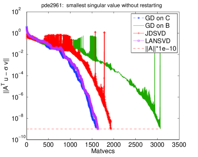
(a) unrestarted

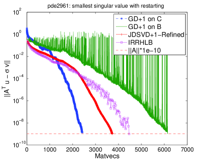
(b) restarted

Fig. 1: Comparing convergence speed of eigenmethods on $C$, $B$, LBD, and JDSVD in both unrestarted and restarted case for matrix pde2961. LANSVD implements LBD without restarting [22] while IRRHLB is currently the most advanced LBD method with implicit restarting [19].

Figure 1(a) demonstrates the relative convergence behavior of these unrestarted methods seeking the smallest singular value of a sample matrix. Only the outer iteration of JDSVD is used (inner iterations = 0). The results agree with the above analysis. The convergence speed of LBD is the same as GD on $C$. JDSVD is slower than LBD or GD but faster than GD on $B$ which is about twice as slow as LBD.

These methods will inevitably be used with restarting. Because LBD, JDSVD, and GD on $B$ extract interior spectral information from the subspaces, critical directions may be dropped during restarting, causing significant convergence slow downs and irregular behavior. The use of harmonic or refined Ritz projections during restart help ameliorate this problem up to a point. However, the problem is still an interior one. In contrast, GD+k on $C$ should see a far smaller effect on its convergence.

Figure 1(b) reflects the above and the advantage of solving an extreme eigenproblem with GD+k. The only disadvantage is the limited accuracy because of the squared conditioning of $C$. Thus, a natural idea is to apply another phase to refine the accuracy until user requirements are satisfied. Instead of iterative refinement, we claim that a second stage eigensolver on $B$ is more efficient.

2.4 Necessary eigensolver features

Our goal is to develop a method that solves large, sparse singular value problems with unprecedented efficiency, robustness, and accuracy. This requires eigensolvers with a certain set of features. First, the eigensolver should be able to use preconditioning because very slow convergence is a limiting factor for seeking smallest singular triplets. Second, large problem size suggests the use of advanced restarting techniques so that limiting memory does not impede convergence. Third, the eigensolver of the second stage should be able to exploit the good quality of the several singular vectors and singular values computed in the first stage. Fourth, the eigensolver on $B$ can benefit from refined or Harmonic Ritz procedures for computing interior eigenvalues.

The state-of-the-art package PRIMME (PReconditioned Iterative MultiMethod Eigensolver) [34] implements the GD+k and JDQMR methods that satisfy most of the above requirements and provides a host of additional features. With a few modifications we have developed our method on top of PRIMME. However, appropriate eigensolvers from other packages could also be used.

3 Developing the two stage strategy

We develop PHSVDS, a two-stage SVD meta-method that first gets a fast solution of the eigenvalue problem on $C$ to the best accuracy possible, and then resolves the remaining accuracy with an eigensolver on $B$. We discuss and automate issues of accuracy, convergence tolerance, initial guesses, and interior eigenvalues of $B$.

3.1 The first stage of PHSVDS

Although an eigensolver on $C$ can be much faster than other methods, the residual norms of the eigenvalues involve $\|C\|=\|A\|^{2}$. Thus achieving the required numerical accuracy may not be possible.

Let $(\sigma,u,v)$ be a targeted singular triplet of $A$ and $(\tilde{\sigma}^{2},\tilde{v})$ the approximating Ritz pair from an eigenmethod working on $C$. Using the approximation $\tilde{u}=A\tilde{v}/\tilde{\sigma}$, we can write the following four residuals:

(9) $$\begin{array}[]{llll}r_{v}=A\tilde{v}-\tilde{\sigma}\tilde{u},&r_{u}=A^{T}\tilde{u}-\tilde{\sigma}\tilde{v},&r_{C}=C\tilde{v}-\tilde{\sigma}^{2}\tilde{v},&r_{B}=B\left[\begin{array}[]{c}\tilde{v}\\ \tilde{u}\end{array}\right]-\tilde{\sigma}\left[\begin{array}[]{c}\tilde{v}\\ \tilde{u}\end{array}\right].\end{array}$$

Typically a singular triplet is considered converged when $\|r_{v}\|$ and $\|r_{u}\|$ are less than a given tolerance. Since our eigenvalue methods work on $C$ and $B$ we need to relate the above quantities. First, it is easy to see that $r_{C}=A^{T}(A\tilde{v})-\tilde{\sigma}^{2}\tilde{v}=\tilde{\sigma}A^{T}\tilde{u}-\tilde{\sigma}^{2}\tilde{v}=\tilde{\sigma}r_{u}$. To relate to the norm of the residual of the second stage note that $\|r_{B}\|^{2}=(\|r_{v}\|^{2}+\|r_{u}\|^{2})/(\|\tilde{v}\|^{2}+\|\tilde{u}\|^{2}).$ If the Ritz vector is normalized, $\|\tilde{v}\|=1$, we also obtain $\|\tilde{u}\|=\|A\tilde{v}/\tilde{\sigma}\|=1$ and $r_{v}=0$. Bringing it all together (see also [39, 24]),

(10) $$\|r_{u}\|=\frac{\|r_{C}\|}{\tilde{\sigma}}=\|r_{B}\|\sqrt{2}.$$

Given a user requirement $\|r_{u}\|<\delta~{}\|A\|$, the normal equations and the augmented methods should be stopped when $\|r_{C}\|<\delta~{}\tilde{\sigma}~{}\|A\|$ and $\|r_{B}\|<\delta~{}\|A\|/\sqrt{2}$ respectively. A common stopping criterion for eigensolvers is $\|r_{C}\|<\delta_{C}\|C\|$, so we must provide $\delta_{C}=\delta~{}\tilde{\sigma}/\|A\|$. In floating point arithmetic this may not be achievable since $\|r_{C}\|$ can only be guaranteed to achieve $O(\|C\|\epsilon_{mach})$ [28]. Thus, we use

(11) $$\delta_{C}=\max\left(\delta~{}\tilde{\sigma}/{\|A\|},\epsilon_{mach}\right)$$

as the criterion for the normal equations.

First, note that for the largest $\sigma_{n}$, $\delta_{C}=\delta$ and thus full residual accuracy is achievable with the normal equations. Since $\sigma\approx\tilde{\sigma}$, based on the Bauer-Fike bound, $|\sigma^{2}-\tilde{\sigma}^{2}|\approx|\sigma-\tilde{\sigma}|(2\tilde{\sigma})\leq\|r_{C}\|<\delta_{C}\|A\|^{2}=\tilde{\sigma}\delta\|A\|$ and thus $|\sigma-\tilde{\sigma}|\leq\delta\|A\|/2$ so the singular values are as accurate as can be expected.

This does not hold for smaller, and in particular the smallest few, eigenvalues. Thus, if the user requires $\delta<{\|A\|}\epsilon_{mach}/\tilde{\sigma}$, PHSVDS first makes full use of the first stage and then switches to the second stage working on $B$ to resolve the remaining accuracy of $O(\tilde{\sigma}/\|A\|)<\kappa(A)^{-1}$. For not too ill conditioned matrices, most of the time is then spent on the more efficient first stage.

A second, more subtle issue involves the accuracy of the Ritz vectors from $C$ which are used as initial guesses to $B$. We have observed that even though their residual norms are below the desired tolerance, the convergence of the interior eigenvalues in $B$ is sometimes (but not often) irregular, with long plateaus, and might not be able to reach machine precision. This occurs when the eigenvalues are highly clustered. On the other hand, it does not occur when only one eigenvalue is sought, which implies that it has to do with the sensitivity of interior eigenvalues to the nearby eigenvectors that we pass as initial guesses [26]. Therefore, before we start stage two, we perform a complete Rayleigh Ritz procedure with the converged eigenvectors of $C$. Providing the new Ritz vectors as initial guesses completely cures this problem.

To understand the problem as well as the solution, consider the decomposition of the smallest Ritz vector $\tilde{u}_{1}$ on the exact eigenvectors of $C$, $\tilde{u}_{1}=c_{1}u_{1}+\sum_{i=2}^{n}c_{i}u_{i}$. On exit from the first stage, its residual satisfies $\|r_{\tilde{u}_{1}}\|<\|C\|\delta_{C}$, and from Bauer-Fike it also holds, $\sqrt{1-c_{1}^{2}}<\|C\|\delta_{C}$ and $c_{i}\leq\|C\|\delta_{C}$. Therefore, if we omit second and higher order terms, the Rayleigh quotient and the residual of $\tilde{u}_{1}$ can be written as:

(12) $$\mu=\frac{\tilde{u}_{1}^{T}A\tilde{u}_{1}}{\tilde{u}_{1}^{T}\tilde{u}_{1}}=\lambda_{1}+\sum\limits_{i=2}^{n}(\frac{c_{i}}{c_{1}})^{2}\lambda_{i},\qquad r_{\tilde{u}_{1}}=A\tilde{u}_{1}-\mu\tilde{u}_{1}\approx\sum\limits_{i=2}^{n}c_{i}(\lambda_{i}-\lambda_{1})u_{i}.$$

As a result of the convergence behavior of iterative methods, the $c_{i}$ tend to be larger for nearby eigenpairs, and fall drastically as $i$ increases. Then, from (12), the accuracy of $\mu$ is dominated by nearby $(c_{i}/c_{1})^{2}$. The post-processing Rayleigh-Ritz uses the $k$ nearby converged Ritz vectors, recomputes the projection with less floating point errors, and rearranges the directions to produce smaller $c_{i},i=2,\ldots,k$, and thus better Ritz values. Of course, the additional Rayleigh-Ritz cannot improve the residual norms without the incorporation of new information in the basis. Even in floating point arithmetic, the improvements are minimal. This is evident also in (12) where $r_{\tilde{u}_{1}}$ depends on the $c_{i}$ linearly, so the effect of improving the nearby $c_{i}$ is small. Figure 2 shows these effects on a matrix that presented the original problem.

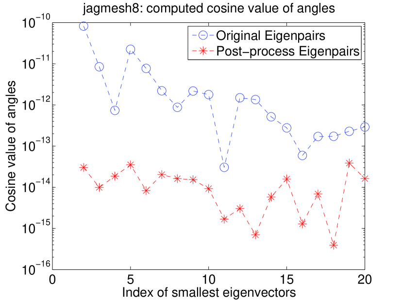
Smallest eigenvalue accuracy Original 3.1E-13 Post-processing 1.9E-16 Smallest residual norm Original 4.1E-13 Post-processing 1.3E-13

Fig. 2: The cosine of angles ($c_{i}=\tilde{u}_{1}^{T}u_{i},i=2,\ldots,19$) between the smallest exact eigenvectors and the smallest Ritz vector before and after pre-processing. The table compares the accuracy of the Rayleigh quotient and the residual norm for $\tilde{u}_{1}$ before and post-processing for matrix jagmesh8.

In the second stage, the improvements on $c_{i}$ translate to a starting search space of better quality, and thus better Ritz (or harmonic Ritz) pairs for the interior eigenvalue problem. Algorithm 1 summarizes the interaction with the first stage eigensolver.

Algorithm 1 PHSVDS first stage

1:  Call an eigesolver on $C$ to compute the required ($\tilde{\sigma}_{i}^{2},\tilde{v}_{i})$ eigenpairs

2:  Eigensolver convergence test uses dynamic tolerance $\delta_{C}=\max\left(\delta_{user}\frac{\tilde{\sigma}_{i}}{\tilde{\sigma}_{n}},\epsilon_{mach}\right)$, where $\tilde{\sigma}_{n}$ and $\tilde{\sigma}_{i}$ are its current largest and targeted Ritz values

3:  If requested, perform Rayleigh-Ritz on the returned Ritz vector basis

3.2 The second stage of PHSVDS

An eigensolver such as GD+k can be used also to compute interior eigenvalues of $B$ close to a given set of shifts. However, the availability of accurate initial guesses and shifts from the first phase suggest that an inner-outer iterative eigenmethod, such as JDQMR, might be preferable.

We argue that solving an eigenvalue problem on matrix $B$ with an approximate eigenspace as initial guess is a better approach than iterative refinement [10, 7]. First, with iterative refinement, eigenvectors are improved one by one without any synergy from the nearby subspace information. In contrast, a subspace eigensolver provides global convergence to all desired pairs. Second, an inner-outer eigensolver such as JDQMR stops the inner linear solver dynamically and near-optimally to avoid exiting too early (which increases the number of outer iterations) or iterating too long (which increases the number of inner iterations). We are not familiar with similar implementations for iterative refinement. Third, iterative refinement for clustered interior eigenvalues may not be able to converge to the desired high accuracy due to the lack of proper deflation strategies [1], both at the linear solver and at the outer iteration. Naturally, a well designed eigensolver that employs locking and blocking techniques is more robust to address these problems. Finally, we point out that the correction equation of the Jacobi-Davidson method applied on $B^{T}$,

(13) $$(I-ww^{T})(B^{T}-\mu I)(I-ww^{T})\tilde{t}=\tilde{\sigma}w-B^{T}w,$$

where $w^{T}=\left[u^{T}v^{T}\right]$ is equivalent to the iterative refinement proposed in [10] ([15]). Therefore, JDQMR enjoys the benefits of both eigensolvers and iterative refinement.

Using the eigenvector approximations $\tilde{v}_{i},\tilde{u}_{i}=A\tilde{v}_{i}/\tilde{\sigma}_{i}$ from the first stage, we form initial guesses to insert in the search space of the JDQMR on $B$. If the guesses are less than the minimum restart size, we fill the rest of the positions with a Lanczos space from the first targeted eigenvector. In addition, we provide the eigenvalue approximations from the first stage, which are typically very accurate because of Hermiticity, as shifts to JDQMR. However, the problems with seeking interior eigenvalues are accentuated in the maximally indefinite case of SVD problems. Spurious Ritz values can cause Ritz vectors to fail to converge [36] or to have a detrimental effect during restart when major eigenvector components may be discarded and need to be recovered [25, 26, 32]. We have addressed these problems as follows.

First, we observed that sometimes eigenvector approximations that are introduced initially in the search space but have not been targeted yet may degrade in quality or even be displaced. Thus, when an eigenvector converges and is locked out of the search space, we re-introduce the initial guess of the next vector to be targeted. This resulted in significant improvement in robustness and often in convergence speed.

Second, we introduced an efficient implementation of the refined projection that minimizes the residual $\|BVy-\tilde{\sigma}Vy\|$ for a given $\tilde{\sigma}$ over the search space $V$ [17, 36]. Because the shifts $\tilde{\sigma}$ are accurate, a harmonic Ritz procedure is not necessary, and the refined one is expected to give the best approximation for the targeted eigenpair. Our refined projection is similar to the one in [16, 25] which produces refined Ritz vectors for all required eigenvectors (not just the closest to $\tilde{\sigma}$). Since $\tilde{\sigma}$ remains constant, there is no need to perform a QR factorization of $BV-\tilde{\sigma}V$ at every step. Instead, as part of Gram-Schmidt, we update the factorization matrices $Q$ and $R$ with a new column. A full QR factorization is only needed at restart. Then, following [36], we compute the refined Ritz vectors by solving the small SVD problem with $R$, and replace the targeted Ritz value with the Rayleigh quotient of the first refined Ritz vector.

Algorithm 2 PHSVDS second stage: necessary enhancements in Jacobi-Davidson

1:  Initial shifts $\tilde{\sigma}_{i}$, initial vectors $[\tilde{v}_{i}\ ;A\tilde{v}_{i}/\tilde{\sigma}_{i}],i=1,...,k$,  $qr\_full=1,~{}j=s+1$

2:  Build an orthonormal basis $V$ of $[K_{s-k}(B,\tilde{v}_{1}),\tilde{v}_{i}]$. Set $t$ as the Lanczos residual

3:  while all $k$ eigenvalues have not converged do

4:     Orthonormalize $t$ against $V$. Update $v_{j}=t,w_{j}=Bv_{j},H_{:,j}=V^{T}w_{j}$

5:     if $qr\_{full}==1$ then

6:        $W-\tilde{\sigma}_{1}V=QR,\ qr\_{full}=0$

7:     else

8:        During orthogonalization update $QR$ by one-column

9:     end if

10:     Compute eigendecomposition $H=S\Theta S^{T}$ with $\theta_{j}$ ordered by closeness to $\tilde{\sigma}_{1}$

11:     Compute SVD decomposition of $R=U\Sigma S^{T}$, Rayleigh quotient $\theta_{1}=s_{1}^{T}Hs_{1}$

12:     If $(\sigma_{i},[v_{i};u_{i}])$ converged, lock, and re-introduce $[\tilde{v}_{i+1}\ ;A\tilde{v}_{i+1}/\tilde{\sigma}_{i+1}]$ into $V$

13:     If restarting, set $qr\_{full}=1$

14:     Obtain the next vector $t=Prec(r)$ (e.g., by solving the correction equation)

15:  end while

Solving the small SVD problem in each iteration for only the targeted shift reduces the cost of the refined procedure considerably, making it similar to the cost of computing the Ritz vectors. However, the quality of non-targeted refined Ritz vectors reduces with the distance of their Rayleigh quotient from $\tilde{\sigma}$, so they may not be as effective in a block algorithm. Yet, these approximations have the desirable property of monotonic convergence as claimed in [16, 25] and also observed in our experiments. This added robustness for JDQMR more than justifies the small additional cost. Algorithm 2 summarizes the second stage modifications in the context of JD.

3.3 Outline of the implementation

We have implemented the PHSVDS meta-method as a MATLAB function on top of PRIMME. This allowed us flexibility for algorithmically tuning the two stages and experimenting with various eigensolvers. We first developed a MATLAB MEX interface for PRIMME, which exposes its full functionality to a broader class of users, who can now take advantage of MATLAB’s built-in matrix times block-of-vectors operators and preconditioners. Its user interface is similar to MATLAB eigs and it is fully tunable. Many of the enhancements, such as the refined projection method or a user provided stopping criterion, were implemented directly in PRIMME and will be part of its next release. We are currently working on a native C implementation of PHSVDS in PRIMME.

PHSVDS expects an input matrix $A$, or a matrix function that performs matrix-vector operations with $A$ and $A^{T}$, or directly with $B$ and/or $C$. Then, it sets up the matrix-vector functions and calls Algorithm 1. The returned approximations are provided as initial guesses to Algorithm 2. One exception is when the singular value is extremely small or zero, so the first stage yields no accuracy for $\tilde{u}_{i}$. In this extreme case, it is better to choose $\tilde{u}_{i}$ as a random vector. For tiny and highly clustered singular values, eigensolvers with locking and block features are preferable.

4 Preconditioning in PHSVDS

The shift-invert technique is sometimes thought of as a form of preconditioning. If a factorization of $A,C$ or $B$ is possible, this is often the method of choice for highly clustered or indefinite eigenproblems. For smallest singular values, MATLAB svds relies solely on shift-invert ARPACK [23] using the LU factorization of $B$. PROPACK [21, 22] uses a QR factorization of $C$. However, for rectangular matrices svds often converges to the zero eigenvalues of $B$ rather than the smallest singular value (see [24]). Our method can also be used in shift-invert mode, assuming the user provides the inverted operator as a matrix-vector. For large matrices, however, preconditioners become a necessary alternative.

JDSVD accepts a preconditioner for a square matrix $A$ or, if $A$ is rectangular, leverages a preconditioner for $B-\tau I$ [15]. SVDIFP includes by default the robust incomplete factorization (RIF) method [6] to provide a preconditioner directly for $C-\tau I$ without forming $C$ [24]. The advantage is that it works seamlessly for both square and rectangular matrices, but RIF may not be the best choice of preconditioner.

PHSVDS accepts any user-provided preconditioning operator that the underlying eigensolver allows. In the most general form, any preconditioner directly for $C$ or $B$ can be used. When $M\approx A$ is available (e.g., the incomplete LU factorization of a square matrix), PHSVDS forms $M^{-1}M^{-T}$ and $[0\ M^{-1};M^{-T}\ 0]$ as the preconditioning operators for the different stages. Moreover, if a preconditioner such as RIF is given, $M\approx C^{-1}$, we can build preconditioners for the second stage as $[0\ AM;MA^{T}\ 0]$. It is not clear in general how to form a preconditioner for $C$ from a preconditioner of $B$.

4.1 A dynamic two stage method with preconditioning

The analysis in Sections 2.2 and 2.3 holds for Krylov methods but it is less meaningful with preconditioners. Clearly, if two different preconditioners are provided for $C$ and $B$ their relative strengths are not known by PHSVDS. But we have also noticed cases where the first stage benefits less than the second stage when a less powerful preconditioner $M$ for $A$ is used to form preconditioners for both $C$ and $B$. If $M$ is ill-conditioned but its near-kernel space does not correspond well to that of $A$, it may work for $B$, but taking $M^{T}M$ produces an unstable preconditioner for $C$ [30]. On the other hand, with a sufficiently good preconditioner, both methods enjoy similar benefits on convergence. If the relative strengths of the provided preconditioner are known, users can choose the two-stage approach or only one of the stages (e.g., the second one). For the general case, we present a method that, based on runtime measurements, switches dynamically between the normal equations and the augmented approach to identify the most effective one for the given preconditioning. This is shown in Algorithm 3.

To estimate the convergence of the two approaches, we run a set of initial tests alternating between running on $C$ and on $B$. Because JDQMR relies on good initial guesses which are not available initially, the dynamic algorithm uses only the GD+k method. Once the algorithm decides on the approach, any eigenmethod that allows for preconditioning can be used. Without loss of generality, we only consider GD+k for our dynamic PHSVDS experiments. The approximations obtained from one run are passed as initial guesses to the next run.

We estimate the convergence rate by measuring the average reduction per iteration of the residual norm. To capture the convergence at different phases of the iterative method, we must switch between the two approaches several times. However, switching too frequently incurs a lot of overhead (rebuilding the initial basis, performing extra Rayleigh-Ritz procedures, and possibly convergence loss from restarting the search space). Switching too infrequently may be wasteful when the preconditioner for $C$ does not work well. Thus, we control the maximum number of iterations for the next GD+k run, $maxIter$. This number is always larger than $initIter$ which is a reasonably small number, i.e., 50. If the same approach is chosen in two successive runs, $maxIter$ doubles. If the approach should be switched, $maxIter$ is reduced more aggressively for the next run (Step 12) to avoid wasting too much time on the wrong approach. If one eigenvalue converges in the initial tests or at least two eigenvalues converge later, we stop the dynamic switching and choose the currently faster approach. If the faster approach is the normal equations, a two-stage method might be necessary to get to full accuracy. Although two or three switches typically suffice to distinguish between approaches, we also limit the number of switches.

Algorithm 3 Dynamic switching between stages for preconditioned PHSVDS

1:  Set $initIter$, $maxSwitch$

2:  $numSwitch=numConverged=j=0,maxIter=initIter,Undecided=true$

3:  Run $initIter$ iterations of an eigensolver (such as GD+k) on $C$ and on $B$ and collect initial average convergence rate of both approaches.

4:  while ($numSwitch<maxSwitch$ and $Undecided$) do

5:     Choose estimated faster approach ($C$ or $B$) for next call

6:     if ($numSwitch==0$ and $numConverged>0)$ or $numConverged>1$ then

7:        undecided = false (Choose faster approach and no more switching)

8:     else

9:        if Same approach is chosen again then

10:           $j=j+1;\ \ maxIter=initIter\ast 2^{j}$

11:        else if Different approach is chosen then

12:           $j=\mbox{floor}(j/2);\ \ maxIter=initIter\ast 2^{j}$

13:        end if

14:     end if

15:     $numSwitch=numSwitch+1$

16:     Call the eigensolver with $maxIter$ and current chosen approach

17:  end while

18:  if All desired singular triplets are found on $B$ then

19:     Return final singular triplets to users

20:  else if All desired singular triplets are found on $C$ then

21:     Return resulting singular triplets to augmented approach

22:  else if Faster approach is on $C$ then

23:     Proceed with the two-stage approach

24:  else if Faster approach is on $B$ then

25:     Continue only with the augmented approach

26:  end if

5 Numerical experiments

Our first two experiments use diagonal matrices to demonstrate the principle of the two stage method and that the method can compute artificially clustered tiny singular values to full accuracy. Then, we conduct an extensive set of experiments for finding the smallest singular values of several matrices. Large singular values are also computed under the shift-invert setting. The matrix set is chosen to overlap with those in other papers in the literature. We compare against several state-of-the-art SVD methods: JDSVD [15, 16], SVDIFP [24], IRRHLB [19], IRLBA [2], lansvd [22], and MATLAB’s svds. All methods are implemented in MATLAB. First, we compute a few of the smallest singular triplets on both square and rectangular matrices without a preconditioner. Then we show show the effect of the dynamic PHSVDS for different quality of preconditioners, and demonstrate that PHSVDS provides faster convergence over other methods on these test matrices as well as on some large scale problems.

All computations are carried out on a DELL dual socket with Intel Xeon processors at 2.93GHz for a total of 16 cores and 50 GB of memory running the SUSE Linux operating system. We use MATLAB 2013a with machine precision $\epsilon=2.2\times 10^{-16}$ and PRIMME is linked to the BLAS and LAPACK libraries available in MATLAB. Our stopping criterion requires that the left and right residuals satisfy,

(14) $$\sqrt{\|r_{u}\|^{2}+\|r_{v}\|^{2}}<\|A\|\delta_{user}.$$

For JDSVD we use the refined projection method as it performed best in our experiments, which is also consistent with [15]. We choose the default for all parameters except for setting ’krylov = 0’ to avoid occasional convergence problems for smallest singular values. For SVDIFP the maximum number of inner iterations can be chosen as fixed or adaptive. We run with both choices and report the best result. Also, we modify slightly the code to use singular triplet residuals as the stopping criterion for SVDIFP instead of the default residual of the normal equations. For IRLBA and IRRHLB, we choose all default parameters as suggested in the code.

All methods start with the same initial guess, ones(min(m,n),1), except for matrix lshp3025 for which a random guess is necessary. We set the maximum number of restarts to 5000 for IRRHLB and IRLBA and to 10000 for JDSVD and PHSVDS. Since SVDIFP can only set a maximum number of iterations for each targeted singular triplet, we report that SVDIFP cannot converge to all desired singular values if its overall number of matrix-vector operations is larger than $(maxBasisSize-k)*5000$. For PHSVDS, we set maxBasisSize=35, minRestartSize=21 and experiment with two $\delta$ tolerances, 1E-8 and 1E-14. For $\delta=$1E-8, PHSVDS does not need to enter the second stage for any of our tests. For the first stage of PHSVDS we use the GD_Olsen_PlusK method. For the second stage, we run experiments with both GD_PlusK and JDQMR. Since our implementation is mainly in C, we compare the number of matrix-vector operations as the primary measurement of the performance. However, we also report execution times which is relevant since matrix-vector, preconditioner, and all BLAS/LAPACK operations are performed by the MATLAB libraries.

Since the numbers of matrix-vector products with $A$ and $A^{T}$ are the same, the tables report as “MV” the number of products with $A$ only. “Sec” is the run time in seconds, and “–” means the method cannot converge to all desired singular values or that the code breaks down. Bargraphs report the ratio of matvecs and time of each method over the PHSVDS method that uses the first stage only or JDQMR in stage two. Ratio values are truncated to less than 10, and empty bar means the same as “–” in the tables.

5.1 PHSVDS for clustered tiny singular values

We illustrate first how our two-stage method works in a seamless manner. We consider a diagonal matrix $A$ = diag([1:10,1000:100:1E6]) and the preconditioner $M$ = $A$ + diag(rand(1,10000)*1E4). In Figure 3, the green and black lines show the convergence behaviors of GD+k on $B$ and $C$ respectively. Indeed, the convergence on $B$ is very slow due to a highly indefinite problem while the accuracy on $C$ stagnates when reaching its limit. The two stage PHSVDS combines the benefits of the two methods, and determines the smallest singular value efficiently and accurately as the magenta line shows.

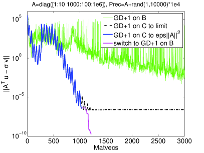
Fig. 3: Two stages of PHSVDS working seamlessly to find smallest singular values accurately.

Next we show how PHSVDS can determine several clustered tiny singular values. Consider the matrix $A$ = diag([1E-14, 1E-12, 1E-8:1E-8:4E-8, 1E-3:1E-3:1]) with identity matrix as a preconditioner. Although locking may be able to determine clustered or multiple singular values, we increase robustness by using a block size of two for the first stage only. We set the user tolerance $\delta_{user}$ = 1E-15 to examine the ultimate accuracy of PHSVDS. As shown in Table 1, PHSVDS is capable of computing all the desired clustered, tiny singular values accurately.

Table 1: Computation of 10 clustered smallest singular values by PHSVDS with block size 2.

$\sigma_{i}$	PHSVDS $\tilde{\sigma}_{i}$	$\|r_{B}\|$
1E-14	9.952750930151887E-15	4.9E-16
1E-12	1.000014102726476E-12	8.9E-16
1E-8	1.000000003582006E-08	6.5E-16
2E-8	2.000000002073312E-08	9.2E-16
3E-8	3.000000000893043E-08	9.0E-16

$\sigma_{i}$	PHSVDS $\tilde{\sigma}_{i}$	$\|r_{B}\|$
4E-8	4.000000001929591E-08	9.2E-16
1E-3	1.000000000000025E-03	9.7E-16
2E-3	1.999999999999956E-03	8.1E-16
3E-3	2.999999999999997E-03	9.1E-16
4E-3	3.999999999999958E-03	9.8E-16

5.2 Without preconditioning

We compare two variants of PHSVDS with four methods, JDSVD, SVDIFP, IRRHLB, and IRLBA on both square and rectangular matrices without preconditioning. Since a good preconditioner is usually not easy to obtain for SVD problems, it is important to examine the effectiveness of a method in this case. We compute $k=1,10$ smallest singular triplets (see [40] for a more detailed and extensive set of results). In order to speed up the convergence of svds, IRRHLB and IRLBA, we compute $k+3$ eigenvalues when $k$ eigenvalues are required. For PHSVDS, we found this is not necessary.

Table 2: Properties of the test matrices. $\gamma_{m}(k)=\min_{i=1}^{k}(gap(\sigma_{i}))$, and $gap(\sigma_{i})=min_{j\neq i}|\sigma_{i}-\sigma_{j}|$.

Matrix	pde2961	dw2048	fidap4	jagmesh8	wang3	lshp3025
order	2961	2048	1601	1141	26064	3025
nnz(A)	14585	10114	31837	7465	77168	120833
$\kappa(A)$	9.5E+2	5.3E+3	5.2E+3	5.9E+4	1.1E+4	2.2E+5
$\|A\|_{2}$	1.0E+1	1.0E+0	1.6E+0	6.8E+0	2.7E-1	7.0E+0
$\gamma_{m}(1)$	8.2E-3	2.6E-3	1.5E-3	1.7E-3	7.4E-5	1.8E-3
$\gamma_{m}(5)$	2.4E-3	2.9E-4	2.5E-4	4.8E-5	1.9E-5	1.8E-4
$\gamma_{m}(10)$	7.0E-4	1.6E-4	2.5E-4	4.8E-5	6.6E-6	2.2E-5

Matrix	well1850	lp_ganges	deter4	plddb	ch	lp_bnl2
rows $m$:	1850	1309	3235	3049	3700	2324
cols $n$:	712	1706	9133	5069	8291	4486
nnz(A)	8755	6937	19231	10839	24102	14996
$\kappa(A)$	1.1E+2	2.1E+4	3.7E+2	1.2E+4	2.8E+3	7.8E+3
$\|A\|_{2}$	1.8E+0	4.0E+0	1.0E+1	1.4E+2	7.6E+2	2.1E+2
$\gamma_{m}(1)$	3.0E-3	1.1E-1	1.1E-1	4.2E-3	1.6E-3	7.1E-3
$\gamma_{m}(5)$	3.0E-3	2.4E-3	8.9E-5	5.1E-5	3.6E-4	1.1E-3
$\gamma_{m}(10)$	2.6E-3	8.0E-5	8.9E-5	2.0E-5	4.0E-5	1.1E-3

We select six square and six rectangular matrices from other research papers [19, 24] and the University of Florida Sparse Matrix Collections [9]. Table 2 lists these matrices along with some of their basic properties. Among them, the matrices pde2961, dw2048, well1850 and lp_ganges have relative larger gap ratios and smaller condition number, and thereby are easy ones. Matrices fidap4, jagmesh8, wang3, deter4, and plddb are hard cases, and matrices lshp3025, ch, and lp_bnl2 are very hard ones. We expect all methods to perform well for solving easy problems. Harder problems tend to magnify the difference between methods.

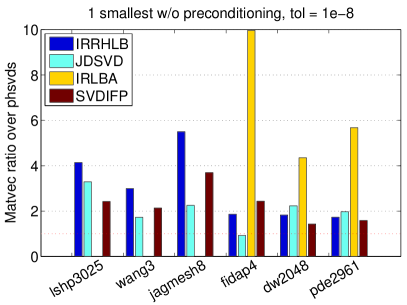
(a) Matvec Ratio

(b) Matvec Ratio

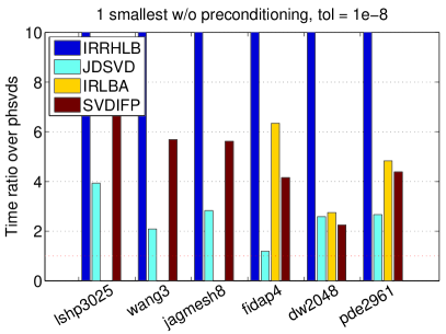
(c) Time Ratio

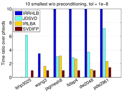
(d) Time Ratio

Fig. 4: Matvec and time ratios over PHSVDS(1st stage only) when seeking 1 and 10 smallest singular triplets of square matrices with user tolerance 1E-8.

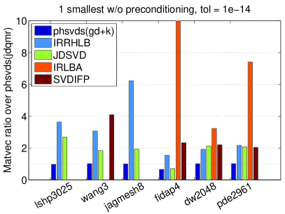
(a) Matvec Ratio

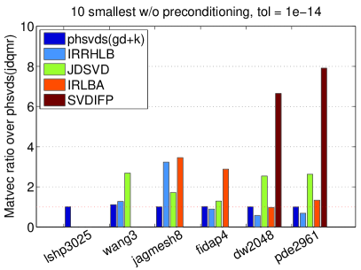
(b) Matvec Ratio

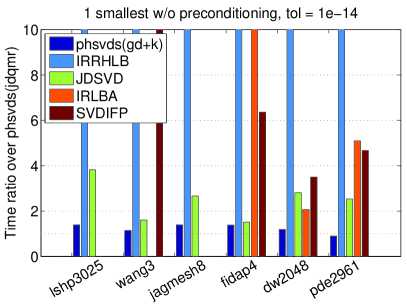
(c) Time Ratio

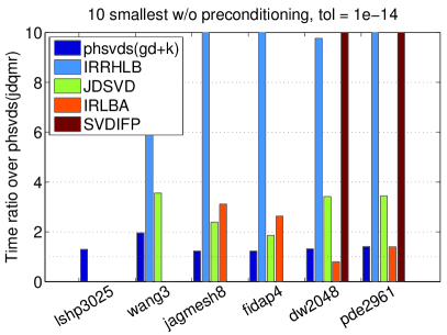
(d) Time Ratio

Fig. 5: Matvec and time ratios over PHSVDS(JDQMR) when seeking 1 and 10 smallest singular triplets of square matrices with user tolerance 1E-14. The PHSVDS(GD+k) variant uses the GD+k eigenmethod in the second stage.

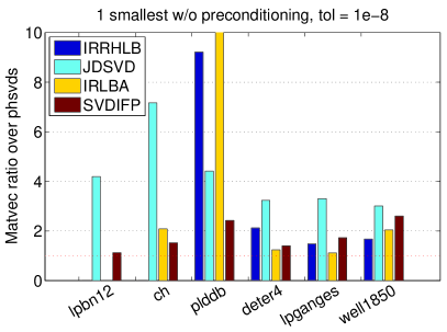
(a) Matvec Ratio

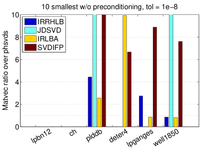
(b) Matvec Ratio

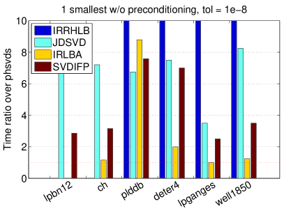
(c) Time Ratio

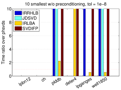
(d) Time Ratio

Fig. 6: Matvec and time ratios over PHSVDS(1st stage only) when seeking 1 and 10 smallest singular triplets of rectangular matrices with user tolerance 1E-8.

(a) Matvec Ratio

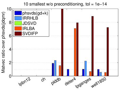
(b) Matvec Ratio

(c) Time Ratio

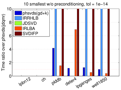
(d) Time Ratio

Fig. 7: Matvec and time ratios over PHSVDS(JDQMR) when seeking 1 and 10 smallest singular triplets of rectangular matrices with user tolerance 1E-14. The PHSVDS(GD+k) variant uses the GD+k eigenmethod in the second stage.

Figures 4, 5, 6 and 7 show that PHSVDS variants converge faster and more robustly than all other methods on both square and rectangular matrices. Specifically, Figure 4 shows that for moderate accuracy the normal equations solved with GD+k are significantly faster. For instance, PHSVDS is at least two or three times faster than other methods when solving hard problems for any number of smallest singular values. In fact, we have noticed that even for moderate accuracy, all other methods are challenged by hard problems, where they are often inefficient or even fail to converge to all desired singular values. When solving easy problems, still PHSVDS is faster than other methods and only IRRHLB can be competitive when seeking 10 singular values. This better global convergence for many eigenvalues is typical of the Lanczos method. The superiority of PHSVDS is a result of using a near-optimal eigenmethod.

Figure 5 shows that the PHSVDS(GD+k) variant is comparable in terms of matvecs to PHSVDS(JDQMR), which is the base of the ratios, but the JDQMR typically requires less time if the matrix is sparse enough. It also shows that despite the slower convergence on the augmented matrix in stage two, the higher accuracy requirement does not help the rest of the methods. For computing 10 eigenpairs, IRRHLB shows a small edge in the number of iterations for two easy cases. However, PHSVDS method never misses eigenvalues, is consistently much faster than all other methods, and significantly faster than IRRHLB in hard cases. SVDIFP is also not competitive, partly due to its inefficient restarting strategy. Interestingly, not only does PHSVDS enjoy better robustness but also its execution time is ten times faster than IRRHLB for the cases where IRRHLB takes fewer matvecs.

Figures 6 and 7 show that the advantage of PHSVDS is even more significant on rectangular matrices. For example, except for the two easy problems well1850 and lp_ganges, PHSVDS is often five or ten times faster than the other methods. The reason is the beneficial use of the first stage, but also because PHSVDS works on $C$ with dimension $\min(m,n)$, which saves memory and computational costs. SVDIFP also shares this advantage. Interestingly, JDQMR converges much faster than GD+k on some hard problems such as plddb, ch and lp_bnl2 in Figure 7. The reason is the availability of excellent shifts from the first stage. We conclude that PHSVDS is the fastest method and sometimes the only method that converges for hard problems without preconditioning.

5.3 With preconditioning

The previous figures show the remarkable difficulty of solving for the smallest singular values. Preconditioning is a prerequisite for practical problems, which limits our choice to PHSVDS, JDSVD and SVDIFP.

We first compare our two stage method and our dynamic two-stage method for two different quality preconditioners. We choose $M=LU$, the factorization obtained from MATLAB’s ILU function on a square matrix $A$ with parameters ’type=ilutp’, ’thresh=1.0’, and varying ’droptol=1E-2’ or ’droptol=1E-3’. Given these two $M$, we form the preconditioners for PHSVDS as $M^{-1}M^{-T}$ and $[0\ M^{-1};M^{-T}\ 0]$. Without loss of generality, PHSVDS chooses GD+k for both stages. We seek ten smallest singular values with tolerance 1E-14.

As shown in Table 3, both variants of PHSVDS can solve the problems effectively with a good preconditioner (’droptol=1E-3’). In this case, the static two stage method is always better than the dynamic one because of the overhead incurred by switching between the two methods. On the other hand, when using the preconditioner with ’droptol=1E-2’, the two stage PHSVDS is slower than the dynamic in some cases, and in the case of lshp3025, much slower. The reason is the inefficiency of the preconditioner in the normal equations. Our dynamic PHSVDS can detect the convergence rate difference and choose the faster method to accomplish the remaining computations. Of course, if this issue is known beforehand, users can bypass the dynamic heuristic and call directly the second stage.

Table 3: Dynamic stage switching PHSVDS (D) vs two stage PHSVDS (P) with two preconditioners: (H)igh quality ILU(1e-3) and (L)ow quality ILU(1E-2). We seek 10 smallest triplets with $\delta=$1E-14.

		pde2961		dw2048		fidap4		jagmesh8		wang3		lshp3025
		MV	Sec	MV	Sec	MV	Sec	MV	Sec	MV	Sec	MV	Sec
H	P	166	0.4	211	0.7	210	1.3	163	0.5	306	5.5	209	3.0
H	D	242	0.4	283	0.7	286	1.4	223	0.6	396	5.5	273	3.6
L	P	258	0.5	673	1.6	813	3.2	990	3.1	736	8.9	7631	132
L	D	307	0.5	668	1.5	1043	3.7	547	1.6	1038	9.6	696	10

Next, we compare the two stage PHSVDS with JDSVD and SVDIFP with a good quality preconditioner. Except for preconditioning, all other parameters remain as before. For the first preconditioner we use MATLAB’s ILU on a square matrix $A$. For the second preconditioner we use the RIF MEX function provided in [24] on a rectangular matrix with ’droptol=1E-3’. The resulting RIF factors $LDL^{T}\approx A^{T}A$, where $D$ is diagonal matrix with 0 and 1 elements, are used to construct the pseudoinverses $M^{-1}=L^{-T}L^{-1}A^{T}$ and $M^{-T}=AL^{-T}L^{-1}$ for preconditioning the second stage of PHSVDS and JDSVD. To obtain uniform behavior across methods, we disable in SVDIFP the parameter ’COLAMD’, which computes an approximate minimum degree column permutation to obtain sparser LU factors. For JDSVD, we try both enabling and disabling the initial Krylov subspace and report the best result.

Table 4: Seeking 1 and 10 smallest singular triplets with ILU, droptol = 1E-3. We report results from both PHSVDS variants: PHSVDS(GD+k) and PHSVDS(JDQMR). We report separately the time for generating the preconditioner and the time for running each method.

	$\delta=$ 1E-8 Matrix:	fidap4		jagmesh8		wang3		lshp3025
	ILU Time:	0.1		0.1		2.8		0.1
$k$	Method	MV	Sec	MV	Sec	MV	Sec	MV	Sec
1	PHSVDS(1st stage only)	15	0.1	13	0.1	46	2.5	19	0.3
1	JDSVD	67	0.7	34	0.3	45	2.0	56	1.5
1	SVDIFP	58	0.4	51	0.2	132	5.7	82	1.7
10	PHSVDS(1st stage only)	117	0.6	91	0.2	185	2.5	122	1.7
10	JDSVD	342	3.1	287	1.4	320	15.7	364	10.5
10	SVDIFP	691	3.0	561	1.2	1179	29.1	1187	21.9

	$\delta=$ 1E-14 Matrix:	fidap4		jagmesh8		wang3		lshp3025
	ILU Time:	0.1		0.1		2.8		0.1
1	PHSVDS(GD+k)	62	0.6	52	0.1	102	1.8	66	0.5
1	PHSVDS(JDQMR)	64	0.3	55	0.1	106	1.1	68	0.5
1	JDSVD	78	1.5	45	0.3	67	3.0	79	1.2
1	SVDIFP	98	0.6	100	0.3	235	8.3	159	2.3
10	PHSVDS(GD+k)	210	1.3	163	0.5	306	5.5	209	3.0
10	PHSVDS(JDQMR)	251	1.2	215	0.5	402	5.0	265	3.5
10	JDSVD	573	5.5	408	1.9	518	14.6	606	26.9
10	SVDIFP	1152	5.4	981	1.9	1991	51.4	1897	29.1

Table 5: Seeking 1 and 10 smallest singular triplets with RIF, droptol = 1E-3. We report results from both PHSVDS variants: PHSVDS(GD+k) and PHSVDS(JDQMR). We report separately the time for generating the preconditioner and the time for running each method.

$\delta=$ 1E-8 Matrix:		fidap4		jagmesh8		deter4		plddb		lp_bnl2
	RIF Time:	1.5		0.5		11.0		0.4		1.6
$k$	Method	MV	Sec	MV	Sec	MV	Sec	MV	Sec	MV	Sec
1	PHSVDS	291	0.4	119	0.1	27	0.2	10	0.1	15	0.1
1	JDSVD	1729	8.9	1311	3.6	122	3.8	67	0.3	89	0.5
1	SVDIFP	513	1.4	622	0.9	142	2.1	29	0.1	49	0.1
10	PHSVDS	1224	1.8	307	0.5	405	2.4	52	0.1	74	0.1
10	JDSVD	8131	39.5	2356	5.7	–	–	–	–	–	–
10	SVDIFP	4359	10.3	3118	4.2	2278	45.4	390	1.0	453	1.0

$\delta=$ 1E-14 Matrix:		fidap4		jagmesh8		deter4		plddb		lp_bnl2
	RIF Time:	1.5		0.5		11.0		0.4		1.6
$k$	Method	MV	Sec	MV	Sec	MV	Sec	MV	Sec	MV	Sec
1	p(GD+k)	521	1.0	207	0.3	82	0.5	45	0.1	66	0.1
1	p(JDQMR)	544	1.0	229	0.2	87	0.4	45	0.1	69	0.1
1	JDSVD	2037	10.5	1410	3.6	188	5.5	122	0.5	134	0.6
1	SVDIFP	843	2.1	990	1.3	221	4.3	48	0.1	63	0.1
10	p(GD+k)	2074	3.2	562	0.8	769	2.5	152	0.5	192	0.5
10	p(JDQMR)	2604	4.9	641	0.9	877	5.3	247	0.5	242	0.5
10	JDSVD	–	–	12057	28.2	–	–	–	–	–	–
10	SVDIFP	7470	15.1	5024	6.1	3705	64.5	748	1.0	862	1.0

Tables 4 and 5 show that a good preconditioner makes the problems tractable, with all three methods solving the problems effectively. Still, in most cases PHSVDS provides much faster convergence and execution time on both square and rectangular matrices. We see that when seeking one smallest singular value with high accuracy, JDSVD takes less iterations for one square matrix (wang3), and SVDIFP is competitive in two rectangular cases (plddb and lp_bnl2). This is because these cases require very few iterations, and the first stage of PHSVDS forces a Rayleigh-Ritz with 21 extra matrix-vector operations. This robust step is not necessary for this quality of preconditioning. If we are allowed to tune some of its parameters (as we did with JDSVD and SVDIFP) PHSVDS does require fewer iterations even in these cases.

5.4 With the shift-invert technique

We report results on seeking 10 smallest eigenvalues with PHSVDS, SVDIFP, svds, and lansvd. Because shift-invert turns an interior to a largest eigenvalue problem, PHSVDS does not need the second stage. svds uses the augmented matrix $B$ for the shift-invert operator, while lansvd computes a QR factorization of $A$. For PHSVDS and SVDIFP we use two different factorizations, an LU and a QR factorization of $A$. All methods get the same basis size of 40, except for lansvd which is an unrestarted LBD code. Thus, lansvd represents an optimal method in terms of convergence, albeit expensive in terms of memory and computation per step. We disable the ’COLAMD’ option in SVDIFP and lansvd, set the SVDIFP shifts to zero, and give a shift 1E-8 to svds. We have instrumented the svds code to return the number of iterations. To facilitate comparisons, we include the LU and QR factorization times in the running times of all methods, but also report them separately. The tolerance is $\delta$ = 1E-10.

Table 6: Seeking 10 smallest singular triplets using shift-invert. LU(A) and QR(A) are the times for LU and QR factorizations of $A$. The time of each method includes the associated factorization time.

$\delta$ = 1E-10	fidap4		jagmesh8		deter4		plddb		lp_bnl2
Method	MV	Sec	MV	Sec	MV	Sec	MV	Sec	MV	Sec
LU(A) time	–	0.02	–	0.01	–	0.01	–	0.01	–	0.01
PHSVDS	31	0.10	26	0.07	167	14.4	47	0.28	35	1.01
SVDIFP	380	0.90	316	0.31	1177	168.4	418	1.92	432	9.3
QR(A) time	–	0.02	–	0.01	–	0.53	–	0.01	–	0.10
PHSVDS	31	0.29	26	0.08	166	9.1	27	0.08	36	0.48
SVDIFP	383	2.24	316	0.37	1177	55.4	418	0.55	432	3.13
svds	73	0.33	61	0.23	–	–	–	–	–	–
lansvd	31	0.37	26	0.24	133	3.3	28	0.23	34	0.43

Table 6 shows that PHSVDS is faster than svds both in convergence and execution time, partly because it works on $C$ which is smaller in size and allows for faster convergence. Note that svds does not work well on rectangular matrices because $B$ becomes singular and cannot be inverted, and if instead a small shift is used, it finds the zero eigenvalues of $B$ first. SVDIFP’s strategy to use an inverted operator as preconditioner does not seem to be as effective. PHSVDS seems to follow closely the optimal convergence of lansvd, although there is high variability in execution times. We believe this is a function not only of the cost of the iterative method but also of the different factorizations used by the two algorithms.

5.5 On large scale problems

We use PHSVDS, SVDIFP, and JDSVD to compute the smallest singular triplet of matrices of order larger than 1 million. Information on these matrices appears in Table 7. We apply the two-stage PHSVDS on all test matrices except thermal2, which is solved with dynamic PHSVDS. The preconditioners are applied similar to our previous experiments with the exception that ILU uses ’thresh=0.1’, and ’udiag=1’. The tolerance is $\delta=1E-12$. The symbol “*” means the method returns results that either did not satisfy the desired accuracy or did not converge to the smallest singular triplet.

Table 7: Basic information of some large scale matrices

Matrix	debr	cage14	thermal2	sls	Rucci1
rows $m$:	1048576	1505785	1228045	1748122	1977885
cols $n$:	1048576	1505785	1228045	62729	109900
nnz(A)	4194298	27130349	8580313	6804304	7791168
$\sigma_{1}$	1.11E-20	9.52E-2	1.61E-6	9.99E-1	1.04E-3
$\kappa(A)$	3.60E+20	1.01E+1	7.48E+6	1.30E+3	6.74E+3
Application	undirected	directed	thermal	Least	Least
	graph	graph		Squares	Squares
Preconditioner	No	ILU(0)	ILU(1E-3)	RIF(1E-3)	RIF(1E-3)

Table 8 shows the results without or with various preconditioners. Debr is a numerically singular square matrix. PHSVDS is capable of resolving this more efficiently than JDSVD, while SVDIFP returns early when it detects that it is not likely to converge to the desired accuracy for left singular vector [24]. All methods easily solve problem cage14 with ILU(0), but PHSVDS is much faster. Thermal2 is an ill-conditioned matrix, whose preconditioner turns out to be less effective for $C$ than for $B$. Therefore, SVDIFP has much slower convergence than JDSVD. Thanks to the dynamic scheme, PHSVDS recognizes this deficiency and converges without too many additional iterations, and with the same execution time as JDSVD. However, if we had prior knowledge about the preconditioner’s performance, running only at the second stage gives almost exactly the same matrix-vectors as JDSVD and much lower time. Reducing further the overhead of the dynamic heuristic is part of our current research. JDSVD often fails to converge to the smallest singular value for rectangular matrices since it has difficulty to distinguish them from zero eigenvalues of $B$, as shown in the cases sls and Rucci1. For matrix sls, SVDIFP misconverges to the wrong singular triplet while PHSVDS is successful in finding the correct one. SVDIFP and PHSVDS have similar performance for solving problem Rucci1. In summary, PHSVDS is far more robust and more efficient than either of the other two methods for large problems.

Table 8: Seeking the smallest singular triplet for large scale problems. We report the time of each method including their running time and associated factorization time (PRtime) separately.

$\delta$ = 1E-12		PHSVDS			SVDIFP			JDSVD
Matrix PRtime		MV	Sec	RES	MV	Sec	RES	MV	Sec	RES
debr	—	539	84	3E-12	403*	246*	2E-1	1971	474.6	2E-12
cage14	2E+0	19	11	4E-13	33	28	6E-13	111	185	7E-14
thermal2	3E+3	419	506	7E-12	–	–	4E-9	309	535	4E-12
sls	3E+3	1779	170	1E-09	408*	328*	1E-9	–	–	2E-0
Rucci1	6E+4	4728	1087	7E-12	4649	6464	6E-12	–	–	5E-3

6 Conclusion

In this paper, we present a two stage meta-method, PHSVDS, that computes smallest or largest singular triplets of large matrices. In the first stage PHSVDS solves the eigenvalue problem on the normal equations as a fast way to get sufficiently accurate approximations, and if further accuracy is needed, solves an interior eigenvalue problem from the augmented matrix. We have presented an algorithm and several techniques required both at the meta-method and at the eigenvalue solver level to allow for an efficient solution of the problem. We have motivated the merit of this approach theoretically, and confirmed its performance through an extensive set of experiments.

Our current implementation of PHSVDS is in MATLAB but based on top of the state-of-the-art preconditioned eigensolver PRIMME. Thus, PHSVDS improves on convergence and robustness over other state-of-the-art singular value methods, and can be used on large, real world problems. A native C implementation of PHSVDS as part of PRIMME is planned next.

References

- [1] M. Arioli and J. Scott, Chebyshev acceleration of iterative refinement, Numerical Algorithms, 66 (2014), pp. 591–608.
- [2] James Baglama and Lothar Reichel, Augmented implicitly restarted Lanczos bidiagonalization methods, SIAM Journal on Scientific Computing, 27 (2005), pp. 19–42.
- [3] , Restarted block Lanczos bidiagonalization methods, Numerical Algorithms, 43 (2006), pp. 251–272.
- [4] , An implicitly restarted block Lanczos bidiagonalization method using Leja shifts, BIT Numerical Mathematics, 53 (2013), pp. 285–310.
- [5] Jesse L. Barlow, Reorthogonalization for the Golub–Kahan–Lanczos bidiagonal reduction, Numerische Mathematik, 124 (2013), pp. 237–278.
- [6] Michele Benzi and Miroslav Tuma, A robust preconditioner with low memory requirements for large sparse least squares problems, SIAM Journal on Scientific Computing, 25 (2003), pp. 499–512.
- [7] Michael W. Berry, Large-scale sparse singular value computations, International Journal of Supercomputer Applications, 6 (1992), pp. 13–49.
- [8] Jane Cullum, Ralph A. Willoughby, and Mark Lake, A Lanczos algorithm for computing singular values and vectors of large matrices, SIAM Journal on Scientific and Statistical Computing, 4 (1983), pp. 197–215.
- [9] Timothy A. Davis and Yifan Hu, The University of Florida sparse matrix collection, ACM Trans. Math. Softw., 38 (2011), pp. 1:1–1:25.
- [10] Jack J. Dongarra, Improving the accuracy of computed singular values, SIAM Journal on Scientific and Statistical Computing, 4 (1983), pp. 712–719.
- [11] Gene Golub and William Kahan, Calculating the singular values and pseudo-inverse of a matrix, Journal of the Society for Industrial and Applied Mathematics Series B Numerical Analysis, 2 (1965), pp. 205–224.
- [12] Gene H. Golub, Franklin T. Luk, and Michael L Overton, A block Lanczos method for computing the singular values and corresponding singular vectors of a matrix, ACM Transactions on Mathematical Software (TOMS), 7 (1981), pp. 149–169.
- [13] Gene H. Golub and Charles F. Van Loan, Matrix Computations (3rd Ed.), Johns Hopkins University Press, Baltimore, MD, USA, 1996.
- [14] Gene H. Golub and Qiang Ye, An inverse free preconditioned Krylov subspace method for symmetric generalized eigenvalue problems, SIAM Journal on Scientific Computing, 24 (2002), pp. 312–334.
- [15] Michiel E. Hochstenbach, A Jacobi–Davidson type SVD method, SIAM Journal on Scientific Computing, 23 (2001), pp. 606–628.
- [16] , Harmonic and refined extraction methods for the singular value problem, with applications in least squares problems, BIT Numerical Mathematics, 44 (2004), pp. 721–754.
- [17] Zhongxiao Jia, Refined iterative algorithms based on Arnoldi’s process for large unsymmetric eigenproblems, Linear algebra and its applications, 259 (1997), pp. 1–23.
- [18] Zhongxiao Jia and Datian Niu, An implicitly restarted refined bidiagonalization Lanczos method for computing a partial singular value decomposition, SIAM journal on matrix analysis and applications, 25 (2003), pp. 246–265.
- [19] , A refined harmonic Lanczos bidiagonalization method and an implicitly restarted algorithm for computing the smallest singular triplets of large matrices, SIAM Journal on Scientific Computing, 32 (2010), pp. 714–744.
- [20] Effrosyni Kokiopoulou, C. Bekas, and E. Gallopoulos, Computing smallest singular triplets with implicitly restarted Lanczos bidiagonalization, Applied numerical mathematics, 49 (2004), pp. 39–61.
- [21] Rasmus Munk Larsen, Lanczos bidiagonalization with partial reorthogonalization, DAIMI Report Series, 27 (1998).
- [22] , Combining implicit restarts and partial reorthogonalization in Lanczos bidiagonalization, SCCM, Stanford University, (2001).
- [23] Richard B. Lehoucq, Danny C. Sorensen, and Chao Yang, ARPACK users’ guide: solution of large-scale eigenvalue problems with implicitly restarted arnoldi methods, (1998).
- [24] Qiao Liang and Qiang Ye, Computing singular values of large matrices with an inverse-free preconditioned Krylov subspace method, Electronic Transactions on Numerical Analysis, 42 (2014), pp. 197–221.
- [25] Ronald B. Morgan, Computing interior eigenvalues of large matrices, Linear Algebra and its Applications, 154 (1991), pp. 289–309.
- [26] Ronald B. Morgan and Min Zeng, Harmonic projection methods for large non-symmetric eigenvalue problems, Numerical Linear Algebra with Applications, 5 (1998), pp. 33–55.
- [27] Chris C. Paige, Beresford N. Parlett, and Henk A Van der Vorst, Approximate solutions and eigenvalue bounds from Krylov subspaces, Numerical linear algebra with applications, 2 (1995), pp. 115–133.
- [28] Beresford N. Parlett, The Symmetric Eigenvalue Problem, Prentice-Hall, 1980.
- [29] B. Philippe and M. Sadkane, Computation of the fundamental singular subspace of a large matrix, Linear algebra and its applications, 257 (1997), pp. 77–104.
- [30] Yousef Saad and Maria Sosonkina, Enhanced preconditioners for large sparse least squares problems, Tech. Report UMSI-2001-1, Minnesota Supercomputer Institute, University of Minnesota, 2001.
- [31] J. Shen, G. Strang, and A. J. Wathen, The potential theory of several intervals and its applications, Applied Mathematics and Optimization, 44 (2001), pp. 67–85.
- [32] Gerard LG Sleijpen and Henk A Van der Vorst, A Jacobi–Davidson iteration method for linear eigenvalue problems, SIAM Review, 42 (2000), pp. 267–293.
- [33] Andreas Stathopoulos, Nearly optimal preconditioned methods for hermitian eigenproblems under limited memory. part i: Seeking one eigenvalue, SIAM Journal on Scientific Computing, 29 (2007), pp. 481–514.
- [34] Andreas Stathopoulos and James R. McCombs, PRIMME: Preconditioned iterative multimethod eigensolver: Methods and software description, ACM Trans. Math. Softw., 37 (2010), pp. 21:1–21:30.
- [35] Andreas Stathopoulos, Yousef Saad, and Kesheng Wu, Dynamic thick restarting of the Davidson, and the implicitly restarted Arnoldi methods, SIAM Journal on Scientific Computing, 19 (1998), pp. 227–245.
- [36] Gilbert W. Stewart, Matrix Algorithms Volume 2: Eigensystems, Society for Industrial and Applied Mathematics, 2001.
- [37] Lloyd N. Trefethen and David Bau III, Numerical Linear Algebra, Society for Industrial and Applied Mathematics, 1997.
- [38] Kesheng Wu and Horst Simon, Thick-restart Lanczos method for large symmetric eigenvalue problems, SIAM Journal on Matrix Analysis and Applications, 22 (2000), pp. 602–616.
- [39] Lingfei Wu and Andreas Stathopoulos, Enhancing the PRIMME eigensolver for computing accurately singular triplets of large matrices, Tech. Report WM-CS-2014-03, Department of Computer Science, College of William and Mary, 2014.
- [40] , PRIMME_SVDS: A preconditioned SVD solver for computing accurately singular triplets of large matrices based on the PRIMME eigensolver, Tech. Report WM-CS-2014-06, Department of Computer Science, College of William and Mary, 2014.