Second-order coding rates for pure-loss bosonic channels

Abstract

A pure-loss bosonic channel is a simple model for communication over free-space or fiber-optic links. More generally, phase-insensitive bosonic channels model other kinds of noise, such as thermalizing or amplifying processes. Recent work has established the classical capacity of all of these channels, and furthermore, it is now known that a strong converse theorem holds for the classical capacity of these channels under a particular photon-number constraint. The goal of the present paper is to initiate the study of second-order coding rates for these channels, by beginning with the simplest one, the pure-loss bosonic channel. In a second-order analysis of communication, one fixes the tolerable error probability and seeks to understand the back-off from capacity for a sufficiently large yet finite number of channel uses. We find a lower bound on the maximum achievable code size for the pure-loss bosonic channel, in terms of the known expression for its capacity and a quantity called channel dispersion. We accomplish this by proving a general “one-shot” coding theorem for channels with classical inputs and pure-state quantum outputs which reside in a separable Hilbert space. The theorem leads to an optimal second-order characterization when the channel output is finite-dimensional, and it remains an open question to determine whether the characterization is optimal for the pure-loss bosonic channel.

1 Introduction

Perhaps the oldest question in quantum information theory was to determine the classical capacity of optical communication channels with quantum effects taken into account [14]. Early work of Holevo in the 1970s represented progress towards its answer [19], but this question remained unsolved for some time—it was only with the advent of quantum computation in the 1990s that interest renewed in it. The next major steps were taken by Hausladen et al. [15] and then Holevo [20] and Schumacher and Westmoreland [27] (HSW), who established a general coding theorem for classical communication over quantum channels. A practically relevant class of channels consists of the phase-insensitive bosonic channels [39], which serve as a model of optical communication. The first contribution towards understanding communication over bosonic channels was from Ozawa and Yuen [44]. Their paper established an upper bound on the classical capacity of a noiseless bosonic channel, which they also showed to be achievable via Shannon’s well-known capacity theorem [30] and so-called “number-state” coding. Holevo and Werner then provided a lower bound on the classical capacity of all phase-insensitive bosonic channels by considering coherent-state coding ensembles and applying the HSW theorem to this case [21]. Later, Giovannetti et al. significantly extended the work of Ozawa and Yuen in [44] by completely characterizing the classical capacity of a pure-loss bosonic channel [11].

In recent work, a full solution to the original question has now been given. In particular, Giovannetti et al. have established the classical capacity of all phase-insensitive bosonic channels [12]. Furthermore, Roy Bardhan et al. [1], building on prior work in [2, 25], have proven that a strong converse theorem holds for the classical capacity of these channels under a particular photon-number constraint, so that the classical capacity of these channels represents a very sharp dividing line between communication rates that are achievable and unachievable.

Let $M^{\ast}(\mathcal{P},\varepsilon)$ denote the maximum number of messages that can be transmitted over a channel$~{}\mathcal{P}$ with failure probability no larger than $\varepsilon\in\left(0,1\right)$. The quantity $\log M^{\ast}(\mathcal{P},\varepsilon)$ is known as the $\varepsilon$-one-shot capacity of $\mathcal{P}$. For $\mathcal{P}$ a bosonic channel, let $M^{\ast}(\mathcal{P},N_{S},\varepsilon)$ denote the same quantity when subject to a photon-number constraint, with $N_{S}\in[0,\infty)$. We can then consider evaluating the quantity $M^{\ast}(\mathcal{P}^{\otimes n},N_{S},\varepsilon)$, i.e., when the sender and receiver are allowed $n$ independent uses of the channel $\mathcal{P}$. When the channel $\mathcal{P}$ is a phase-insensitive bosonic channel, the lower bound on the classical capacity from coherent-state coding schemes [21] combined with the strong converse and the photon-number constraint given in [1] allows us to conclude that

$$\lim_{n\rightarrow\infty}\frac{1}{n}\log M^{\ast}\left(\mathcal{P}^{\otimes n},N_{S},\varepsilon\right)=C(\mathcal{P},N_{S}),$$ (1.1)

where $C\left(\mathcal{P},N_{S}\right)$ is the classical capacity (also referred to as Holevo capacity) of $\mathcal{P}$ with signaling photon number $N_{S}$. Although the statement in (1.1) is helpful for understanding the information transmission properties of phase-insensitive bosonic channels (in particular, that the capacity $C(\mathcal{P},N_{S})$ plays the role of a sharp threshold in the large $n$ limit), it does little to help us understand what rates are achievable for a given $n$ and fixed error $\varepsilon$, the regime in which we are interested in practice.

2 Summary of Results

The main objective of the present paper is to initiate the study of the second-order characterization of bosonic channel capacity, in an effort to understand the newly raised question given above. To do so, we focus on the pure-loss bosonic channel $\mathcal{N}_{\eta}$, which is a completely positive trace preserving map resulting from the following Heisenberg evolution:

$$\hat{b}=\sqrt{\eta}\hat{a}+\sqrt{1-\eta}\hat{e}.$$ (2.1)

In the above, $\eta\in\left[0,1\right]$ is the channel transmissivity, roughly representing the average fraction of photons that make it from sender to receiver, and $\hat{a}$, $\hat{b}$, and $\hat{e}$ correspond to the field mode operators for the channel’s input, output, and environment, respectively. Typically, one makes some kind of photon-number constraint on the input of this channel so that it cannot exceed $N_{S}\in[0,\infty)$. Without doing so, i.e., letting $N_{S}=\infty$, the capacity is infinite for any fixed $n$ and $\varepsilon\neq 0$.

The main result of this paper is the following lower bound on $\log M^{\ast}\left(\mathcal{N}_{\eta}^{\otimes n},N_{S},\varepsilon\right)$:

$$\log M^{\ast}\left(\mathcal{N}_{\eta}^{\otimes n},N_{S},\varepsilon\right)\geq ng(\eta N_{S})+\sqrt{nv(\eta N_{S})}\Phi^{-1}(\varepsilon)+O(\log n),$$ (2.2)

whenever $n$ is large enough so that $n\propto 1/\varepsilon^{2}$ and there is a mean photon-number constraint. Here $g(\eta N_{S})$ is the entropy of a thermal state with mean photon number $\eta N_{S}$:

$$g(x)\equiv\left(x+1\right)\log\left(x+1\right)-x\log x.$$ (2.3)

Also, $\Phi^{-1}\left(\varepsilon\right)$ is the inverse of the cumulative normal distribution function, so that $\Phi^{-1}\left(\varepsilon\right)\leq 0$ if and only if $\varepsilon\leq 1/2$.

It is known from [11] that $g(\eta N_{S})$ is equal to the classical capacity of the pure-loss bosonic channel subject to a mean photon-number constraint, and that it is the strong converse capacity when subject to a different photon-number constraint [43]. The quantity $v(\eta N_{S})$ is the entropy variance of a thermal state, which we show is equal to

$$v(x)\equiv x\left(x+1\right)\left[\log\left(x+1\right)-\log\left(x\right)\right]^{2}.$$ (2.4)

By inspecting (2.2), we can see that the entropy variance characterizes the back-off from capacity at a fixed error $\varepsilon$ and for a sufficiently large yet finite $n$.

The above lower bound is reminiscent of the following second-order asymptotic expansion of $\log M^{\ast}\left(\mathcal{N}^{\otimes n},\varepsilon\right)$ when $\mathcal{N}$ is a discrete memoryless classical channel:

$$\log M^{\ast}\left(\mathcal{N}^{\otimes n},\varepsilon\right)=nC\left(\mathcal{N}\right)+\sqrt{nV_{\varepsilon}\left(\mathcal{N}\right)}\Phi^{-1}\left(\varepsilon\right)+O\left(\log n\right),$$ (2.5)

where $C\left(\mathcal{N}\right)$ is the classical channel capacity and $V_{\varepsilon}\left(\mathcal{N}\right)$ is a channel parameter now known as the channel dispersion [26]. The formula in (2.5) was first identified by Strassen [32] and later refined by Hayashi [17] and Polyanskiy et al. [26]. See [33] for an excellent review of these developments. In recent work, Tomamichel and Tan have identified that a form similar to (2.5) characterizes $\log M^{\ast}\left(\mathcal{N}^{\otimes n},\varepsilon\right)$ for $\mathcal{N}$ a quantum channel with classical input and a finite-dimensional quantum output [36]. Their main contribution was to establish the inequality $\leq$ in (2.5) for such channels for which the input alphabet is finite (see [36] for details regarding other channels). The inequality $\geq$ in (2.5) follows directly from a “one-shot” coding theorem of Wang and Renner [38], which builds on earlier work of Hayashi and Nagaoka [18], along with an asymptotic analysis due to Li [23] and Tomamichel and Hayashi [35]. One would like to directly apply these results in order to recover the bound in (2.2), but cannot do so because the pure-loss bosonic channel has an infinite-dimensional output. A careful study of the analysis in [23] and [35] reveals that their techniques are not directly applicable for our setting here.

The rest of this paper proceeds as follows. The next section establishes some notation and definitions used throughout the rest of the paper. Section 4 establishes a one-shot coding theorem for pure-state classical-quantum channels (those with classical input and a pure-state classical output). This one-shot coding theorem states that a quantity known as the $\varepsilon$-spectral inf-entropy [16] gives a lower bound on $\log M^{\ast}\left(W,\varepsilon\right)$ for any pure-state classical-quantum channel $W$. Section 5 then demonstrates how to combine this result with the Berry-Esseen central limit theorem to recover a second-order lower bound of the form in (2.2) for pure-state classical-quantum channels. We apply this result to the particular case of a pure-loss bosonic channel in Section 6, recovering the result stated in (2.2), and we compare the achievable rates with conventional detection strategies in Section 6.2. Finally, we conclude with a summary and some open questions for future research.

3 Preliminaries

3.1 The $\varepsilon$-spectral inf-entropy

Let $\rho$ be a density operator, which is a bounded positive semi-definite operator on a separable Hilbert space, such that its trace is equal to one. We often use the shorthand $\phi\equiv\left|\phi\right\rangle\left\langle\phi\right|$ for a pure state $\left|\phi\right\rangle$. We denote a channel with classical input$~{}x$ and quantum output $\left|\phi_{x}\right\rangle$ as follows:

$$W:x\rightarrow\left|\phi_{x}\right\rangle,$$ (3.1)

and we refer to it throughout as a pure-state cq (classical-quantum) channel. Note that the input alphabet can be continuous and the output Hilbert space can be infinite-dimensional, as is the case for the pure-loss bosonic channel that we consider in this paper.

Let a spectral decomposition of $\rho$ be given by

$$\rho=\sum_{z}p_{Z}\left(z\right)\left|\psi_{z}\right\rangle\left\langle\psi_{z}\right|,$$ (3.2)

where $\left\{p_{Z}\left(z\right)\right\}$ is a probability distribution and $\left\{\left|\psi_{z}\right\rangle\right\}$ is a countable orthonormal basis. Let $\gamma\geq 0$ and

$$\Pi_{\gamma}\equiv\left\{\rho\leq 2^{-\gamma}I\right\},$$ (3.3)

so that $\Pi_{\gamma}$ projects onto a subspace $\mathcal{T}_{\gamma}$ of the support of $\rho$ spanned by eigenvectors of $\rho$ with eigenvalues less than$~{}2^{-\gamma}$:

$$\mathcal{T}_{\gamma}\equiv\text{span}\left\{\left|\psi_{z}\right\rangle:p_{Z}\left(z\right)\leq 2^{-\gamma}\right\}.$$ (3.4)

Let $\underline{H}_{s}^{\varepsilon}\left(\rho\right)$ denote the $\varepsilon$-spectral inf-entropy of $\rho$, defined for $\varepsilon\in\left[0,1\right)$ as [16]

$$\underline{H}_{s}^{\varepsilon}\left(\rho\right) \equiv\sup\left\{\zeta:\text{Tr}\left\{\rho\Pi_{\zeta}\right\}\geq 1-\varepsilon\right\}$$ (3.5)

$$=\sup\left\{\zeta:\text{Tr}\left\{\rho\left(I-\Pi_{\zeta}\right)\right\}\leq\varepsilon\right\}.$$ (3.6)

From these definitions, if we set $\gamma=\underline{H}_{s}^{\varepsilon}\left(\rho\right)$, we can conclude that

$$\text{Tr}\left\{\Pi_{\gamma}\rho\right\}\geq 1-\varepsilon.$$ (3.7)

By employing the spectral decomposition of $\rho$ in (3.2), we can also express (3.6) as

$$\underline{H}_{s}^{\varepsilon}\left(\rho\right)=\sup\left\{\zeta:\Pr_{Z}\left\{-\log p_{Z}\left(Z\right)\leq\zeta\right\}\leq\varepsilon\right\}.$$ (3.8)

3.2 Central-limit-theorem bounds

Let $\Phi\left(x\right)$ denote the cumulative distribution function of a standard normal random variable:

$$\Phi\left(x\right)\equiv\frac{1}{\sqrt{2\pi}}\int_{-\infty}^{x}dy\ \exp\left\{-y^{2}/2\right\},$$ (3.9)

and let $\Phi^{-1}\left(\varepsilon\right)$ denote its inverse: $\Phi^{-1}\left(\varepsilon\right)\equiv\sup\left\{a\in\mathbb{R}:\Phi\left(a\right)\leq\varepsilon\right\}$ (this is the usual inverse for $\varepsilon\in\left(0,1\right)$ and extends to take values $\pm\infty$ when $\varepsilon$ is outside that interval). The Berry-Esseen theorem gives a quantitative statement of convergence in the central limit theorem (see, e.g., [9, Section XVI.5]) and plays a prominent role in understanding the second-order asymptotics of information-processing tasks [26, 35, 36, 33].

Theorem 1 (Berry-Esseen)

Let $X_{1}$, …, $X_{n}$ be a sequence of independent and identically distributed real-valued random variables, each with mean $\mu$, variance $\sigma^{2}>0$, and finite third absolute moment, i.e., $T\equiv\mathbb{E\{}\left|X_{1}\right|^{3}\}<\infty$. Then the cumulative distribution function of the sum of the standardized versions of $X_{1}$, …, $X_{n}$ converges uniformly to that of a standard normal random variable, with convergence rate $O\left(1/\sqrt{n}\right)$. That is, for all $n\geq 1$:

$$\sup_{x\in\mathbb{R}}\left|\Pr\left\{\frac{1}{\sigma\sqrt{n}}\sum_{i=1}^{n}\left[X_{i}-\mu\right]\leq x\right\}-\Phi\left(x\right)\right|\leq\frac{T}{\sigma^{3}\sqrt{n}}.$$ (3.10)

The constant in the upper bound in (3.10) is due to [37]. When evaluated for a tensor-power state$~{}\rho^{\otimes n}$, an application of the Berry-Esseen theorem to (3.8) gives the following asymptotic expansion for$~{}\underline{H}_{s}^{\varepsilon}\left(\rho^{\otimes n}\right)$:

$$\underline{H}_{s}^{\varepsilon}\left(\rho^{\otimes n}\right)=nH(\rho)+\sqrt{nV(\rho)}\Phi^{-1}\left(\varepsilon\right)+O\left(1\right),$$ (3.11)

where the quantum entropy $H(\rho)$ and quantum entropy variance $V(\rho)$ are defined as

$$H(\rho) \equiv-\text{Tr}\left\{\rho\log\rho\right\}=\mathbb{E}_{Z}\left\{-\log p_{Z}\left(Z\right)\right\},$$ (3.12)

$$V(\rho) \equiv\text{Tr}\left\{\rho\left[-\log\rho-H\left(\rho\right)\right]^{2}\right\}=\text{Var}_{Z}\left\{-\log p_{Z}\left(Z\right)\right\}.$$ (3.13)

(See, e.g., [35, Section IV] for more details.)

3.3 Communication codes for pure-state cq channels

This section establishes some notation for classical communication over a pure-state cq channel$~{}W$, given by (3.1). The goal is to transmit classical messages from a sender to a receiver by making use of $W$, where the messages are labeled by the elements of a set $\mathcal{M}$. Without loss of generality, any classical communication protocol for $W$ has the following form: the sender encodes a classical message $m$ into a letter $x$ that is accepted at the input of the channel. Let $\mathcal{E}:\mathcal{M\rightarrow X}$ denote the encoding map and let $x\left(m\right)$ denote the codeword corresponding to message $m$. The sender then transmits the codeword $x\left(m\right)$ over $W$ to the receiver. Subsequently, the receiver performs a positive operator-valued measure (POVM) $\{\Lambda_{m}\}_{m\in\mathcal{M}}$ on the system in his possession (i.e., the operators $\Lambda_{m}$ are positive semi-definite and sum to the identity). This yields a classical register $\widehat{M}$ which contains his inference $\hat{m}\in\mathcal{M}$ of the message sent by the sender. The above defines a classical code for the cq channel $W$, which consists of a triple

$$\mathcal{C}\equiv\left\{\mathcal{M},\mathcal{E},\{\Lambda_{m}\}_{m\in\mathcal{M}}\right\}.$$ (3.14)

The size of a code is denoted as $\left|\mathcal{C}\right|=|\mathcal{M}|$. The average probability of error for $\mathcal{C}$ on $W$ is

$$p_{\text{err}}(W,\mathcal{C})\equiv\Pr[\widehat{M}\neq M]=1-\frac{1}{|\mathcal{M}|}\sum_{m}\text{Tr}\left\{\Lambda_{m}\phi_{x\left(m\right)}\right\}.$$ (3.15)

The following quantity denotes the maximum size of a code for transmitting classical information over a single use of $W$ with average probability of error at most $\varepsilon$.

Definition 2

Let $\varepsilon\in(0,1)$ and $W$ be a pure-state cq channel as given in (3.1). We define

$$M^{\ast}(W,\varepsilon)\equiv\max\left\{m\in\mathbb{N}\,:\,\exists\mathcal{C}:\left|\mathcal{C}\right|=m\wedge p_{\operatorname{err}}(W,\mathcal{C})\leq\varepsilon\right\},$$ (3.16)

where $\mathcal{C}$ is a code as prescribed in (3.14).

4 One-shot coding for pure-state cq channels

Theorem 3 below establishes a one-shot lower bound on the maximum achievable code size $M^{\ast}\left(W,\varepsilon\right)$ for a pure-state cq channel $W$ and error $\varepsilon\in\left(0,1\right)$. The main advantage of this theorem over [38, Theorem 1] is that our lower bound on $\log M^{\ast}\left(W,\varepsilon\right)$ is given directly in terms of the $\varepsilon$-spectral inf-entropy, rather than the hypothesis testing divergence. This in turn allows us to apply the theorem directly in conjunction with the Berry-Esseen theorem, in order to establish the lower bound in (2.2).

Theorem 3

Let $W$ be a pure-state cq channel as given in (3.1), let $p_{X}\left(x\right)$ be a probability distribution over the channel’s input alphabet, and let $\rho$ be the expected density operator at the output:

$$\rho\equiv\mathbb{E}_{X\sim p_{X}}\left\{\left|\phi_{X}\right\rangle\left\langle\phi_{X}\right|\right\}.$$ (4.1)

Then there exists a codebook for communication over $W$ with average error probability no larger than $\varepsilon\in(0,1)$, such that the maximum number of bits $\log M^{\ast}\left(W,\varepsilon\right)$ one can send obeys

$$\log M^{\ast}\left(W,\varepsilon\right)\geq\underline{H}_{s}^{\varepsilon-\eta}\left(\rho\right)-\log\left(4\varepsilon/\eta^{2}\right),$$ (4.2)

where $\eta\in(0,\varepsilon)$.

Proof. Suppose that $\rho$ has a spectral decomposition as in (3.2), and let $\gamma$ be a parameter such that

$$\gamma=\underline{H}_{s}^{\varepsilon-\eta}\left(\rho\right).$$ (4.3)

We now discuss a coding scheme.

Codebook Construction. Before communication begins, the sender and receiver agree upon a codebook. We allow them to select a codebook randomly according to the distribution $p_{X}\left(x\right)$. So, for every message $m\in\mathcal{M}\equiv\left\{1,\ldots,M\right\}$, generate a codeword $x\left(m\right)$ randomly and independently according to $p_{X}\left(x\right)$.

Decoding. Transmitting the codeword $x\left(m\right)$ over the channel $x\rightarrow\left|\phi_{x}\right\rangle$ leads to the state $\left|\phi_{x\left(m\right)}\right\rangle$ at the receiver’s end. Let $\left|\phi_{x\left(m\right)}^{\gamma}\right\rangle$ be a unit vector resulting from projecting the codeword $\left|\phi_{x\left(m\right)}\right\rangle$ onto the subspace given in (3.4):

$$\left|\phi_{x\left(m\right)}^{\gamma}\right\rangle\equiv\frac{1}{\left\|\Pi_{\gamma}\left|\phi_{x\left(m\right)}\right\rangle\right\|_{2}}\Pi_{\gamma}\left|\phi_{x\left(m\right)}\right\rangle.$$ (4.4)

Upon receiving the quantum codeword $\left|\phi_{x\left(m\right)}\right\rangle$, the receiver performs a square-root measurement [3, 4] with the following elements, in an attempt to decode the message $m$:

$$\Lambda_{m}^{\gamma}\equiv\left(\sum_{m^{\prime}}\phi_{x\left(m^{\prime}\right)}^{\gamma}\right)^{-1/2}\phi_{x\left(m\right)}^{\gamma}\left(\sum_{m^{\prime}}\phi_{x\left(m^{\prime}\right)}^{\gamma}\right)^{-1/2}.$$ (4.5)

Error Analysis. The error when decoding the $m$th codeword is

$$\text{Tr}\left\{\left(I-\Lambda_{m}^{\gamma}\right)\phi_{x\left(m\right)}\right\}.$$ (4.6)

Recall the following operator inequality [18, Lemma 2]

$$I-\Lambda_{m}^{\gamma}\leq c_{\text{I}}\left(I-\phi_{x\left(m\right)}^{\gamma}\right)+c_{\text{II}}\sum_{m^{\prime}\neq m}\phi_{x\left(m^{\prime}\right)}^{\gamma},$$ (4.7)

where

$$c_{\text{I}}\equiv 1+c,\ \ \ \ \ \ \ \ c_{\text{II}}\equiv 2+c+c^{-1},$$ (4.8)

and $c$ is a strictly positive number. Applying this operator inequality leads to the following upper bound on the error:

$$\text{Tr}\left\{\left(I-\Lambda_{m}^{\gamma}\right)\phi_{x\left(m\right)}\right\}\leq c_{\text{I}}\text{Tr}\left\{\left(I-\phi_{x\left(m\right)}^{\gamma}\right)\phi_{x\left(m\right)}\right\}+c_{\text{II}}\sum_{m^{\prime}\neq m}\text{Tr}\left\{\phi_{x\left(m^{\prime}\right)}^{\gamma}\phi_{x\left(m\right)}\right\}.$$ (4.9)

Taking the expectation $\mathbb{E}_{\mathcal{C}}$ over the random choice of code gives the following bound:

$$\mathbb{E}_{\mathcal{C}}\left\{\text{Tr}\left\{\left(I-\Lambda_{m}^{\gamma}\right)\phi_{X\left(m\right)}\right\}\right\}\leq c_{\text{I}}\ \mathbb{E}_{\mathcal{C}}\left\{\text{Tr}\left\{\left(I-\phi_{X\left(m\right)}^{\gamma}\right)\phi_{X\left(m\right)}\right\}\right\}\\ +c_{\text{II}}\ \mathbb{E}_{\mathcal{C}}\left\{\sum_{m^{\prime}\neq m}\text{Tr}\left\{\phi_{X\left(m^{\prime}\right)}^{\gamma}\phi_{X\left(m\right)}\right\}\right\}.$$ (4.10)

By the way that the code is chosen, we have that

$$\mathbb{E}_{\mathcal{C}}\left\{\text{Tr}\left\{\left(I-\phi_{X\left(m\right)}^{\gamma}\right)\phi_{X\left(m\right)}\right\}\right\} =\mathbb{E}_{X\left(m\right)}\left\{\text{Tr}\left\{\left(I-\phi_{X\left(m\right)}^{\gamma}\right)\phi_{X\left(m\right)}\right\}\right\},$$ (4.11)

$$\mathbb{E}_{\mathcal{C}}\left\{\sum_{m^{\prime}\neq m}\text{Tr}\left\{\phi_{X\left(m^{\prime}\right)}^{\gamma}\phi_{X\left(m\right)}\right\}\right\} =\sum_{m^{\prime}\neq m}\mathbb{E}_{X\left(m\right),X\left(m^{\prime}\right)}\left\{\text{Tr}\left\{\phi_{X\left(m^{\prime}\right)}^{\gamma}\phi_{X\left(m\right)}\right\}\right\}.$$ (4.12)

Consider that

$$\mathbb{E}_{X\left(m\right)}\left\{\text{Tr}\left\{\phi_{X\left(m\right)}^{\gamma}\phi_{X\left(m\right)}\right\}\right\} =\mathbb{E}_{X\left(m\right)}\left\{\frac{1}{\left\langle\phi_{X^{n}\left(m\right)}\right|\Pi_{\gamma}\left|\phi_{X\left(m\right)}\right\rangle}\text{Tr}\left\{\Pi_{\gamma}\phi_{X\left(m\right)}\Pi_{\gamma}\phi_{X\left(m\right)}\right\}\right\}$$ (4.13)

$$=\mathbb{E}_{X\left(m\right)}\left\{\frac{\left[\left\langle\phi_{X\left(m\right)}\right|\Pi_{\gamma}\left|\phi_{X\left(m\right)}\right\rangle\right]^{2}}{\left\langle\phi_{X\left(m\right)}\right|\Pi_{\gamma}\left|\phi_{X\left(m\right)}\right\rangle}\right\}$$ (4.14)

$$=\mathbb{E}_{X\left(m\right)}\left\{\left\langle\phi_{X\left(m\right)}\right|\Pi_{\gamma}\left|\phi_{X\left(m\right)}\right\rangle\right\}$$ (4.15)

$$=\mathbb{E}_{X\left(m\right)}\left\{\text{Tr}\left\{\Pi_{\gamma}\phi_{X\left(m\right)}\right\}\right\}$$ (4.16)

$$=\text{Tr}\left\{\Pi_{\gamma}\rho\right\}$$ (4.17)

$$\geq 1-\left(\varepsilon-\eta\right).$$ (4.18)

The first equality follows from (4.4). The last equality follows from (4.1) and the last inequality from (3.7). We can then bound the error term in the first line of (4.10) as follows:

$$\mathbb{E}_{X\left(m\right)}\left\{\text{Tr}\left\{\left(I-\phi_{X\left(m\right)}^{\gamma}\right)\phi_{X\left(m\right)}\right\}\right\}\leq\varepsilon-\eta.$$ (4.19)

We can bound each of the errors in the second line of (4.10) as

$$\mathbb{E}_{X\left(m\right),X\left(m^{\prime}\right)}\left\{\text{Tr}\left\{\phi_{X\left(m^{\prime}\right)}^{\gamma}\phi_{X\left(m\right)}\right\}\right\}$$

$$=\mathbb{E}_{X\left(m\right),X\left(m^{\prime}\right)}\left\{\frac{1}{\left\langle\phi_{X\left(m^{\prime}\right)}\right|\Pi_{\gamma}\left|\phi_{X\left(m^{\prime}\right)}\right\rangle}\text{Tr}\left\{\Pi_{\gamma}\phi_{X\left(m^{\prime}\right)}\Pi_{\gamma}\phi_{X\left(m\right)}\right\}\right\}$$ (4.20)

$$=\mathbb{E}_{X\left(m^{\prime}\right)}\left\{\frac{1}{\left\langle\phi_{X\left(m^{\prime}\right)}\right|\Pi_{\gamma}\left|\phi_{X\left(m^{\prime}\right)}\right\rangle}\text{Tr}\left\{\Pi_{\gamma}\phi_{X\left(m^{\prime}\right)}\Pi_{\gamma}\mathbb{E}_{X\left(m\right)}\left\{\phi_{X\left(m\right)}\right\}\right\}\right\}$$ (4.21)

$$=\mathbb{E}_{X\left(m^{\prime}\right)}\left\{\frac{1}{\left\langle\phi_{X\left(m^{\prime}\right)}\right|\Pi_{\gamma}\left|\phi_{X\left(m^{\prime}\right)}\right\rangle}\text{Tr}\left\{\phi_{X\left(m^{\prime}\right)}\Pi_{\gamma}\rho\Pi_{\gamma}\right\}\right\}$$ (4.22)

$$\leq 2^{-\gamma}\mathbb{E}_{X\left(m^{\prime}\right)}\left\{\frac{1}{\left\langle\phi_{X\left(m^{\prime}\right)}\right|\Pi_{\gamma}\left|\phi_{X\left(m^{\prime}\right)}\right\rangle}\text{Tr}\left\{\phi_{X\left(m^{\prime}\right)}\Pi_{\gamma}\right\}\right\}$$ (4.23)

$$=2^{-\gamma}.$$ (4.24)

The first equality follows from (4.4). The second equality follows from the independence of the codewords corresponding to different messages. The third equality follows from (4.1) and cyclicity of the trace. The first inequality is a result of $\Pi_{\gamma}\rho\Pi_{\gamma}\leq 2^{-\gamma}\Pi_{\gamma}$, which follows from the definition of $\Pi_{\gamma}$ in (3.3). The bounds in (4.19) and (4.20)-(4.24) then lead to the following upper bound on the expectation of the average error probability:

$$\mathbb{E}_{\mathcal{C}}\left\{\sum_{m}\text{Tr}\left\{\left(I-\Lambda_{m}^{\gamma}\right)\phi_{X\left(m\right)}\right\}\right\}\leq c_{\text{I}}\left(\varepsilon-\eta\right)+c_{\text{II}}\ M\ 2^{-\gamma}.$$ (4.25)

So this means there exists a particular codebook with average error probability less than

$$c_{\text{I}}\left(\varepsilon-\eta\right)+c_{\text{II}}\ M\ 2^{-\gamma}.$$ (4.26)

We would like to have this quantity equal to $\varepsilon$, so we pick $M$ and $\eta$ such that this is possible:

$$\varepsilon=c_{\text{I}}\left(\varepsilon-\eta\right)+c_{\text{II}}\ M\ 2^{-\gamma}.$$ (4.27)

We rewrite in terms of $\log M$, so that

$$\log M=\gamma+\log\left(\frac{\varepsilon-c_{\text{I}}\left(\varepsilon-\eta\right)}{c_{\text{II}}}\right)=\underline{H}_{s}^{\varepsilon-\eta}\left(\rho\right)+\log\left(\frac{\varepsilon-c_{\text{I}}\left(\varepsilon-\eta\right)}{c_{\text{II}}}\right).$$ (4.28)

Choosing $c=\eta/\left(2\varepsilon-\eta\right)$ and substituting for $c_{\text{I}}$ and $c_{\text{II}}$ then leads to

$$\log M=\underline{H}_{s}^{\varepsilon-\eta}\left(\rho\right)-\log\left(4\varepsilon/\eta^{2}\right),$$ (4.29)

which concludes the proof of the theorem.   

Remark 4

The square-root measurement in (4.5) is different from the original square-root measurement constructed in [15] because we take the extra step of normalizing the vectors after projecting them to the subspace $\mathcal{T}_{\gamma}$. When employing an error analysis along the lines given above, this normalization appears to be essential in order to recover the correct second-order asymptotics, at least for the case of cq pure-state channels with finite-dimensional outputs. That is, the lower bound in (5.3) matches the upper bound in [36] for this case.

Remark 5

It would be desirable to establish Theorem 3 when the receiver employs a sequential quantum decoder [24, 13]. In particular, it would be desirable if the receiver were able to decode the pure-loss bosonic channel by performing the “vacuum-or-not” measurement discussed in [42]. However, there are two obstacles to be overcome. First, the standard tool for error analysis of a sequential quantum decoder is the “non-commutative union bound” [28, Lemma 3], but the version of it given in [28] does not feature an optimization over a “$c$” variable, as is the case with the operator inequality in (4.7). Second, the normalization of the vectors in (4.4) excludes us from employing the vacuum-or-not measurement. Sen has recently informed us that it is possible to overcome the first obstacle by modifying [28, Lemma 3] in order to allow for a “$c$” variable which can be optimized [29]. One might be able to overcome the second obstacle with an error analysis improving upon ours.

5 Second-order coding rates for memoryless channels

Of interest in applications is a memoryless pure-state cq channel $W^{\otimes n}$, defined by

$$W^{\otimes n}:x_{1}\cdots x_{n}\rightarrow\left|\phi_{x_{1}}\right\rangle\otimes\cdots\otimes\left|\phi_{x_{n}}\right\rangle.$$ (5.1)

For such a channel, we apply Theorem 3, picking codewords according to an i.i.d. distribution $\prod_{i=1}^{n}p_{X}(x_{i})$, to find that it is possible to transmit the following number of bits with average probability of error no larger than $\varepsilon\in\left(0,1\right)$:

$$\log M^{\ast}\left(W^{\otimes n},\varepsilon\right)\geq\underline{H}_{s}^{\varepsilon-\eta}\left(\rho^{\otimes n}\right)-\log\left(4\varepsilon/\eta^{2}\right).$$ (5.2)

By a direct application of the Berry-Esseen theorem as discussed in Section 3.2, choosing $\eta=\frac{1}{\sqrt{n}}$ and $n$ large enough so that $\varepsilon-\eta>0$, we find that the lower bound in (5.2) expands to

$$\log M^{\ast}\left(W^{\otimes n},\varepsilon\right)\geq nH(\rho)+\sqrt{nV(\rho)}\Phi^{-1}\left(\varepsilon\right)+O\left(\log n\right),$$ (5.3)

where $H(\rho)$ and $V(\rho)$ are defined in (3.12)-(3.13) and we make use of the fact that $\Phi^{-1}$ is a continuously differentiable function (see, e.g., [6, Lemma 3.7]).

Our derivation applies for pure-state cq channels with outputs in a separable Hilbert space. However, note that the lower bound in (5.3) also serves as an upper bound as well for channels with finite-dimensional outputs. This follows because in the finite-dimensional case, we can apply the results of [36], thus establishing the RHS of (5.3) as an optimal second-order characterization in this case.

6 Application to the Pure-Loss Bosonic Channel

We now apply these results to the case of the pure-loss bosonic channel $\mathcal{N}_{\eta}$, defined by the transformation in (2.1). In this case, we can induce a pure-state cq channel from the map in (2.1) by picking a coherent state $\left|\alpha\right\rangle$ [10] parametrized by $\alpha\in\mathbb{C}$ and sending the coherent state over the pure-loss bosonic channel. One key reason why coherent states are good candidates for signaling over this channel is that the channel retains their purity, only reducing their amplitude at the output. That is, the output state is $|\sqrt{\eta}\alpha\rangle$ whenever the input is $\left|\alpha\right\rangle$, where $\eta\in(0,1]$ is the channel transmissivity. So the induced pure-state cq channel is

$$\alpha\rightarrow|\sqrt{\eta}\alpha\rangle.$$ (6.1)

Since $\eta$ is just a scaling factor, we take $\eta=1$ in what follows for simplicity. The memoryless version of this channel is simply

$$\alpha_{1}\cdots\alpha_{n}\rightarrow\left|\alpha_{1}\right\rangle\otimes\cdots\otimes\left|\alpha_{n}\right\rangle.$$ (6.2)

Since all of the codewords are chosen to be coherent states, this leads to coherent states at the output. The distribution to choose the codewords is an i.i.d. extension of the following isotropic, complex Gaussian with variance$~{}N_{S}$:

$$p_{N_{S}}\left(\alpha\right)\equiv\frac{1}{\pi N_{S}}\exp\left\{-\left|\alpha\right|^{2}/N_{S}\right\}.$$ (6.3)

The average state of the ensemble is then $n$ copies of a thermal state $\theta\left(N_{S}\right)$:

$$\theta\left(N_{S}\right)\equiv\int d^{2}\alpha\ p_{N_{S}}\left(\alpha\right)\left|\alpha\right\rangle\left\langle\alpha\right|,$$ (6.4)

which is in fact diagonal in the number basis [10, Sections 2.5 and 3.8], so that

$$\theta\left(N_{S}\right)=\sum_{n=0}^{\infty}\frac{N_{S}^{n}}{\left(N_{S}+1\right)^{n+1}}\left|n\right\rangle\left\langle n\right|.$$ (6.5)

The entropy $H\left(\theta\left(N_{S}\right)\right)$ of the thermal state is equal to

$$H\left(\theta\left(N_{S}\right)\right)=g(N_{S})=\left(N_{S}+1\right)\log\left(N_{S}+1\right)-N_{S}\log N_{S}.$$ (6.6)

As shown in Appendix A, the entropy variance $V\left(\theta\left(N_{S}\right)\right)$ is given by the expression

$$V\left(\theta\left(N_{S}\right)\right)=v(N_{S})=N_{S}\left(N_{S}+1\right)\left[\log\left(N_{S}+1\right)-\log\left(N_{S}\right)\right]^{2}.$$ (6.7)

Thus, from the discussion in the previous section, we can conclude that the number of bits one can send over $n$ uses of a pure-loss bosonic channel with failure probability no larger than $\varepsilon\in\left(0,1\right)$ has the following lower bound for sufficiently large yet finite$~{}n$:

$$\log M^{\ast}\left(\mathcal{N}_{\eta=1}^{\otimes n},N_{S},\varepsilon\right)\geq ng(N_{S})+\sqrt{nv(N_{S})}\Phi^{-1}\left(\varepsilon\right)+O\left(\log n\right).$$ (6.8)

Including the channel loss parameter $\eta\in(0,1]$ explicitly leads to the second-order expansion

$$\log M^{\ast}\left(\mathcal{N}_{\eta}^{\otimes n},N_{S},\varepsilon\right)\geq ng(\eta N_{S})+\sqrt{nv(\eta N_{S})}\Phi^{-1}\left(\varepsilon\right)+O\left(\log n\right).$$ (6.9)

Remark 6

The results in [36] are not sufficient to recover (6.9). The analysis there applies only to channels with finite-dimensional outputs, as where the pure-loss bosonic channel has an infinite-dimensional output space. Furthermore, we should clarify that even though our decoder projects the output space, the projection is onto an infinite-dimensional subspace because we keep only the photon-number states such that their probabilities are smaller than a threshold $2^{-\gamma}$ (and this includes photon-number states with arbitrarily large photon number, yet exponentially small probability).

6.1 Photon-number constraint

The development in the previous section ignores imposing a photon-number constraint, other than choosing the coherent-state codewords according to the distribution $p_{N_{S}}\left(\alpha\right)$. Strictly speaking, we must impose a photon-number constraint on the codebook, or else the capacity is infinite. The usual constraint is to impose a mean photon-number constraint (see, e.g., [21, 11]). However, as shown in [43], a strong converse need not hold under such a constraint. Another photon-number constraint (considered in [43]) is to demand that the average codeword density operator have a large projection onto a photon-number subspace with photon number no larger than $\left\lceil nN_{S}\right\rceil$, where $n$ is the number of channel uses and $N_{S}$ is the energy parameter. Specifically, we might demand that the probability that the average codeword density operator is outside this subspace decreases exponentially with increasing blocklength. Under this constraint, the strong converse holds [43]. We can satisfy this demand and decodability for the receiver by choosing coherent states randomly from an isotropic complex Gaussian distribution with variance $N_{S}-\delta_{1}$, where $\delta_{1}$ is a small strictly positive real. So, as long as the number of bits to transmit is of the order

$$ng\left(N_{S}-\delta_{1}\right)+\sqrt{nv\left(N_{S}-\delta_{1}\right)}\Phi^{-1}\left(\varepsilon^{1+\delta_{2}}\right)+O\left(\log n\right),$$ (6.10)

for $\delta_{2}>0$, then we can guarantee that the probability that the average codeword density operator is outside this subspace decreases exponentially with $n$. Furthermore, we know that the expectation of the average error probability is less than $\varepsilon^{1+\delta_{2}}$. We can then run through the same argument as in [43] to conclude that there exists a code with second-order expansion as given above, such that we meet the photon-number constraint and the receiver can decode with average error probability no larger than $\varepsilon$. We just need $n$ large enough so that

$$\left[C\left(\delta_{1},N_{S}-\delta_{1}\right)\right]^{n/2}+\varepsilon^{\delta_{2}}<1,$$ (6.11)

where the constant $C\left(\delta_{1},N_{S}-\delta_{1}\right)<1$, as specified in [43]. Thus, at the cost of a degradation in the second-order asymptotics, we can meet the photon-number constraint. One might be able to circumvent this degradation by a more advanced approach in which codewords are chosen on the power-limited sphere (see, e.g., [34] for details of this approach in the classical case). However, we leave this for future work.

6.2 Comparison with standard receivers

Heterodyne detection paired with coherent-state encoding is a conventional strategy for communication over a pure-loss bosonic channel (see, e.g., [31]). By this, we mean that the codewords are of the form in (6.2), and the receiver detects every channel output with a heterodyne receiver. The resulting channel from input to output is mathematically equivalent to two parallel classical Gaussian channels, so that the total classical capacity of heterodyne detection is $C_{\mathrm{Het}}(N_{S})=\log_{2}(1+N_{S})$ bits/mode, if the codewords have mean photon number $N_{S}$. In the high photon-number regime, it is well known that the classical capacity of heterodyne detection asymptotically approaches the Holevo capacity $g\left(N_{S}\right)$ as $N_{S}\rightarrow\infty$ [11]. The classical dispersion of the heterodyne detection receiver is given by $v_{\mathrm{Het}}(\eta N_{S})$, where

$$v_{\mathrm{Het}}(x)\equiv\frac{x(x+2)\left(\log_{2}e\right)^{2}}{(x+1)^{2}},$$ (6.12)

which results from applying the classical dispersion of the additive white noise Gaussian channel (see [17, Section IV] or [26, Theorem 54]) to the two parallel channels induced by heterodyne detection. By comparing (6.12) with (6.7), it is straightforward to show that

$$\lim_{N_{S}\rightarrow\infty}\frac{v(N_{S})}{v_{\mathrm{Het}}(N_{S})}=1.$$ (6.13)

This implies that, in the high $N_{S}$ regime, heterodyne detection not only achieves the capacity, but also the second-order expansion (5.3) of the rate as a function of blocklength.

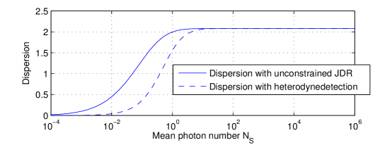
Figure 1: Plots of dispersions $v_{\mathrm{Het}}(N_{S})$ (Heterodyne) and $v(N_{S})$ (optimal JDR) as a function of mean received photon number per mode $N_{S}$.

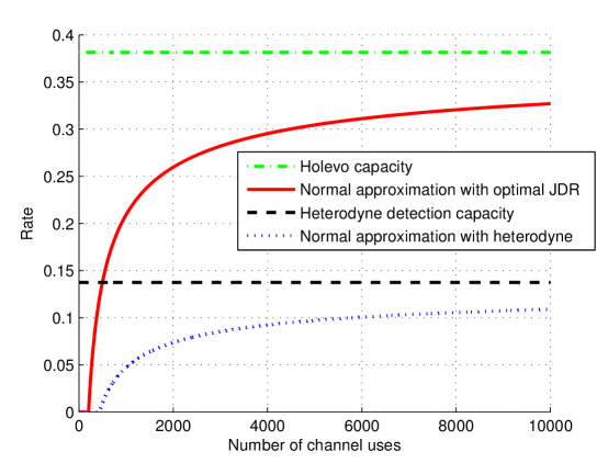
Figure 2: Normal approximation for the optimal JDR and the heterodyne detection receiver at a block error rate threshold of $\varepsilon=10^{-6}$ and with $N_{S}=0.1$.

In Figure 1, we plot $v_{\mathrm{Het}}(N_{S})$ (dashed line) and $v(N_{S})$ (solid line) as a function of mean received photon number per mode $N_{S}$. As expected, the most pronounced difference between the dispersions occurs in the “deep quantum regime,” the extremes of which are for values of $N_{S}$ between $10^{-4}$ and one photon. In Figure 2, we consider a low mean photon number ($N_{S}=0.1$), where there is a gap between the Holevo capacity $g\left(N_{S}\right)$ (blue solid line) and the capacity of heterodyne detection (red solid line), and we show how the rate for the respective receiver assumptions increases with the number $n$ of channel uses, at a block error rate threshold of $\varepsilon=10^{-6}$. However, we stress here that this latter plot is intended only to give the reader a rough sense of which rates are achievable, as they are the “normal approximation,” which is accurate only for sufficiently large $n$.

In the low-photon-number regime, the coherent-state binary phase shift keying (BPSK) modulation $\left\{|\alpha\rangle,|-\alpha\rangle\right\}$, with $|\alpha|^{2}=N_{S}$ suffices to achieve capacity close to the unconstrained-modulation Holevo limit. The Holevo limit of the BPSK constellation is given by

$$C_{\mathrm{BPSK-Holevo}}({N_{S}})=h_{2}\left(\frac{1-\langle-\alpha|\alpha\rangle}{2}\right)=h_{2}\left(\frac{1-e^{-2N_{S}}}{2}\right)\,{\text{bits per mode}},$$ (6.14)

where $h_{2}(x)=-x\log x-(1-x)\log(1-x)$ is the binary entropy function. In units of “nats” per mode, the three dominant terms in the expansion of $C_{\mathrm{BPSK-Holevo}}({N_{S}})$, and the unconstrained-modulation Holevo limit $C_{\mathrm{Ultimate-Holevo}}(N_{S})=g(N_{S})$, in the $N_{S}\ll 1$ regime, are given by

$$C_{\mathrm{Ultimate-Holevo}}(N_{S}) \approx-{N_{S}}\ln{N_{S}}+{N_{S}}+\frac{N_{S}^{2}}{2}\equiv C_{\infty},\,{\text{and}}$$ (6.15)

$$C_{\mathrm{BPSK-Holevo}}({N_{S}}) \approx-{N_{S}}\ln{N_{S}}+{N_{S}}+N_{S}^{2}\ln{N_{S}},$$ (6.16)

which are identical in the first two terms of the expansion. Note also that the photon efficiency (nats per photon) goes as $-\ln N_{S}+1$, which increases without bound as $N_{S}$ decreases towards zero. The maximum capacity attained by the BPSK modulation, when paired with a receiver that detects each BPSK symbol one at a time, is attained by the measurement that discriminates $|\alpha\rangle$ and $\left|-\alpha\right\rangle$ with the minimum probability of error. This minimum error probability is attained by the Dolinar receiver [8], which when used as a receiver for a BPSK modulation, induces a binary symmetric channel of cross-over probability

$$\varepsilon=\left[1-\sqrt{1-|\langle-\alpha|\alpha\rangle|^{2}}\right]/2=\left[1-\sqrt{1-e^{-4N_{S}}}\right]/2.$$ (6.17)

Thus the capacity attained by the best single-symbol measurement $C_{1}=1-h_{2}(\varepsilon)$, the dominant terms in the expansion of which in the $N_{S}\ll 1$ regime, is given by

$$C_{\mathrm{BPSK-Dolinar}}({N_{S}})\approx-2N_{S}+o(N_{S})\equiv C_{1}.$$ (6.18)

It is clear that the photon efficiency caps off at two nats per photon as $N_{S}\rightarrow 0$. Hence, the gap between $C_{1}$ and $C_{\infty}$ widens as $N_{S}$ decreases.

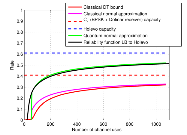
Figure 3: Rate achievable by a BPSK alphabet (in bits per BPSK symbol) at a block error rate threshold of $\varepsilon=10^{-3}$ using the optimal single-symbol receiver and an optimal JDR at mean photon number $N_{S}=0.1783$.

In Figure 3, we consider a BPSK alphabet of mean photon number $N_{S}=|\alpha|^{2}=0.1783$ ($e^{-2N_{S}}=0.7$), and plot the optimal single-symbol receiver capacity $C_{1}$ and the Holevo capacity $C_{\infty}$ (the horizontal red and blue dashed lines). We plot one achievable finite blocklength rate for BPSK coding, shown by the red solid plot, known as the DT (dependency testing) bound [26]. The magenta solid line plots the normal approximation to the second-order rate (capacity minus the dispersion correction term) as a function of the number $n$ of channel uses. For the Holevo capacity, we give a finite-blocklength achievability plot, a bound which derives from the Burnashev-Holevo reliability function (black line) [5]. The green solid line plots the normal approximation to the second-order rate for the BPSK ensemble as a function of the number $n$ of channel uses, i.e., evaluated from (5.3) with $\rho=(|\alpha\rangle\langle\alpha|+\left|-\alpha\right\rangle\left\langle-\alpha\right|)/2$. Comparing the reliability function with $C_{1}$, we see that, for a BPSK constellation with pulses of $\approx 0.18$ photons, for a block error rate target of $\varepsilon=10^{-3}$, a joint-detection receiver will need to act collectively on at least $200$ BPSK symbols in order for the communication rate to increase beyond what is possible by the best symbol-by-symbol receiver strategy.

7 Conclusion

The main results of this paper are a one-shot coding theorem for arbitrary pure-state classical-quantum channels and the application of this theorem to determine second-order coding rates for communication over pure-loss bosonic channels. The latter result is a first step towards understanding the second-order asymptotics of communication over bosonic channels.

There are many open questions to consider going forward from here. First and foremost, it is important to determine whether the formula in (2.2) serves as an upper bound for $\log M^{\ast}\left(\mathcal{N}_{\eta}^{\otimes n},N_{S},\varepsilon\right)$. At the very least, one should impose a photon-number constraint similar to that given in [43]—with a mean photon-number constraint, it is already known that the formula in (2.2) cannot be an upper bound on $\log M^{\ast}\left(\mathcal{N}_{\eta}^{\otimes n},N_{S},\varepsilon\right)$, due to the lack of a strong converse [43, Section 2]. One could also consider extending the achievability results developed here to the case of general phase-insensitive bosonic channels. There is some hope that a complete understanding of the second-order asymptotics could be developed, now that a strong converse theorem has been proven in this setting [1]. Next, one could also consider evaluating the second-order asymptotics of bosonic channels when shared entanglement between sender and receiver is available before communication begins. Some early progress in this direction is in [7] and references therein. Furthermore, there are many quantum information-processing tasks for which a first-order characterization is known (see, e.g., [40, 41] for a summary), and for which some second-order characterizations are now known [35, 36, 22, 6]. One could also consider these tasks in the bosonic setting, which could have more practical applications.

Acknowledgements. We are grateful to Vincent Y. F. Tan, Marco Tomamichel, and Andreas Winter for helpful discussions related to this paper. The ideas for this research germinated in a research visit of SG and MMW to JMR at ETH Zurich in February 2013. SG and MMW are grateful to Renato Renner’s quantum information group at the Institute of Theoretical Physics of ETH Zurich for hosting them during this visit. MMW is grateful for the hospitality of the Quantum Information Processing Group at Raytheon BBN Technologies for subsequent research visits during August 2013 and April 2014. MMW acknowledges startup funds from the Department of Physics and Astronomy at LSU, support from the NSF under Award No. CCF-1350397, and support from the DARPA Quiness Program through US Army Research Office award W31P4Q-12-1-0019. JMR acknowledges support from the Swiss National Science Foundation (through the National Centre of Competence in Research ‘Quantum Science and Technology’ and grant No. 200020-135048) and the European Research Council (grant No. 258932). SG was supported by DARPA’s Information in a Photon (InPho) program, under Contract No. HR0011-10-C-0159.

Appendix A Calculation of the Bosonic Dispersion

This appendix provides justification for the entropy variance formula in (6.7). The key helpful aspect for calculating the dispersion for the pure-loss bosonic channel is that the thermal state is diagonal in the number basis, as given in (6.5). The eigenvalues in (6.5) form a geometric distribution $p\left(1-p\right)^{n}$, where $p\equiv 1/\left(N_{S}+1\right)$. This distribution has mean $\left(1-p\right)/p=N_{S}$ and variance $\left(1-p\right)/p^{2}=N_{S}\left(N_{S}+1\right)$, so that the second moment is $N_{S}\left(N_{S}+1\right)+N_{S}^{2}$. With this, we now calculate the second central moment of the random variable $-\log p_{N}\left(N\right)$:

$$v\left(N_{S}\right) =\sum_{n=0}^{\infty}\frac{1}{N_{S}+1}\left(\frac{N_{S}}{N_{S}+1}\right)^{n}\left|-\log\left(\frac{N_{S}^{n}}{\left(N_{S}+1\right)^{n+1}}\right)-\left[\left(N_{S}+1\right)\log\left(N_{S}+1\right)-N_{S}\log N_{S}\right]\right|^{2}$$ (A.1)

$$=\sum_{n=0}^{\infty}\frac{1}{N_{S}+1}\left(\frac{N_{S}}{N_{S}+1}\right)^{n}\left|\left(n-N_{S}\right)\log\left(N_{S}+1\right)-\left(n-N_{S}\right)\log\left(N_{S}\right)\right|^{2}$$ (A.2)

$$=\sum_{n=0}^{\infty}\frac{1}{N_{S}+1}\left(\frac{N_{S}}{N_{S}+1}\right)^{n}\left|\left(n-N_{S}\right)\left[\log\left(N_{S}+1\right)-\log\left(N_{S}\right)\right]\right|^{2}$$ (A.3)

$$=\sum_{n=0}^{\infty}\frac{1}{N_{S}+1}\left(\frac{N_{S}}{N_{S}+1}\right)^{n}\left(n-N_{S}\right)^{2}\left[\log\left(N_{S}+1\right)-\log\left(N_{S}\right)\right]^{2}$$ (A.4)

$$=\left[\log\left(N_{S}+1\right)-\log\left(N_{S}\right)\right]^{2}\sum_{n=0}^{\infty}\frac{1}{N_{S}+1}\left(\frac{N_{S}}{N_{S}+1}\right)^{n}\left(n^{2}-2nN_{S}+N_{S}^{2}\right)$$ (A.5)

Using the above facts regarding the geometric distribution, we find that the sum evaluates to

$$N_{S}\left(N_{S}+1\right)+N_{S}^{2}-2N_{S}^{2}+N_{S}^{2}=N_{S}\left(N_{S}+1\right),$$ (A.6)

so that the variance is equal to

$$N_{S}\left(N_{S}+1\right)\left[\log\left(N_{S}+1\right)-\log\left(N_{S}\right)\right]^{2}.$$ (A.7)

References

- [1] Bhaskar Roy Bardhan, Raul Garcia-Patron, Mark M. Wilde, and Andreas Winter. Strong converse for the classical capacity of optical quantum communication channels. January 2014. arXiv:1401.4161.
- [2] Bhaskar Roy Bardhan and Mark M. Wilde. Strong converse rates for classical communication over thermal and additive noise bosonic channels. Physical Review A, 89(2):022302, February 2014. arXiv:1312.3287.
- [3] Viacheslav Belavkin. Optimal distinction of non-orthogonal quantum signals. Radio Engineering and Electronic Physics, 20:39–47, 1975.
- [4] Viacheslav Belavkin. Optimal multiple quantum statistical hypothesis testing. Stochastics, 1:315–345, 1975.
- [5] Marat V. Burnashev and Alexander S. Holevo. On reliability function of quantum communication channel. Problems of Information Transmission, 34:97–107, 1998. arXiv:quant-ph/9703013.
- [6] Nilanjana Datta and Felix Leditzky. Second-order asymptotics for source coding, dense coding and pure-state entanglement conversions. March 2014. arXiv:1403.2543.
- [7] Nilanjana Datta, Marco Tomamichel, and Mark M. Wilde. Second-order coding rates for entanglement-assisted communication. May 2014. arXiv:1405.1797.
- [8] Samuel Dolinar. A class of optical receivers using optical feedback. PhD thesis, Massachusetts Institute of Technology, June 1976.
- [9] William Feller. An Introduction to Probability Theory and Its Applications. John Wiley and Sons, 2nd edition edition, 1971.
- [10] Christopher Gerry and Peter Knight. Introductory Quantum Optics. Cambridge University Press, November 2004.
- [11] Vittorio Giovannetti, Saikat Guha, Seth Lloyd, Lorenzo Maccone, Jeffrey H. Shapiro, and Horace P. Yuen. Classical capacity of the lossy bosonic channel: The exact solution. Physical Review Letters, 92(2):027902, January 2004. arXiv:quant-ph/0308012.
- [12] Vittorio Giovannetti, Alexander S. Holevo, and Raúl García-Patrón. A solution of the Gaussian optimizer conjecture. December 2013. arXiv:1312.2251.
- [13] Vittorio Giovannetti, Seth Lloyd, and Lorenzo Maccone. Achieving the Holevo bound via sequential measurements. Physical Review A, 85(1):012302, January 2012. arXiv:1012.0386.
- [14] J. P. Gordon. Noise at optical frequencies; information theory. In P. A. Miles, editor, Quantum Electronics and Coherent Light; Proceedings of the International School of Physics Enrico Fermi, Course XXXI, pages 156–181, Academic Press New York, 1964.
- [15] Paul Hausladen, Richard Jozsa, Benjamin Schumacher, Michael Westmoreland, and William K. Wootters. Classical information capacity of a quantum channel. Physical Review A, 54(3):1869–1876, September 1996.
- [16] Masahito Hayashi. Second-order asymptotics in fixed-length source coding and intrinsic randomness. IEEE Transactions on Information Theory, 54(10):4619–4637, October 2008. arXiv:cs/0503089.
- [17] Masahito Hayashi. Information spectrum approach to second-order coding rate in channel coding. IEEE Transactions on Information Theory, 55(11):4947–4966, November 2009. arXiv:0801.2242.
- [18] Masahito Hayashi and Hiroshi Nagaoka. General formulas for capacity of classical-quantum channels. IEEE Transactions on Information Theory, 49(7):1753–1768, July 2003. arXiv:quant-ph/0206186.
- [19] Alexander S. Holevo. Bounds for the quantity of information transmitted by a quantum communication channel. Problems of Information Transmission, 9(3):177–183, 1973.
- [20] Alexander S. Holevo. The capacity of the quantum channel with general signal states. IEEE Transactions on Information Theory, 44(1):269–273, January 1998.
- [21] Alexander S. Holevo and Reinhard F. Werner. Evaluating capacities of bosonic Gaussian channels. Physical Review A, 63(3):032312, February 2001. arXiv:quant-ph/9912067.
- [22] Wataru Kumagai and Masahito Hayashi. Entanglement concentration is irreversible. Physical Review Letters, 111(13):130407, September 2013. arXiv:1305.6250.
- [23] Ke Li. Second order asymptotics for quantum hypothesis testing. Annals of Statistics, 42(1):171–189, February 2014. arXiv:1208.1400.
- [24] Seth Lloyd, Vittorio Giovannetti, and Lorenzo Maccone. Sequential projective measurements for channel decoding. Physical Review Letters, 106(25):250501, June 2011. arXiv:1012.0106.
- [25] Andrea Mari, Vittorio Giovannetti, and Alexander S. Holevo. Quantum state majorization at the output of bosonic Gaussian channels. Nature Communications, 5:3826, May 2014. arXiv:1312.3545.
- [26] Yury Polyanskiy, H. Vincent Poor, and Sergio Verdú. Channel coding rate in the finite blocklength regime. IEEE Transactions on Information Theory, 56(5):2307–2359, May 2010.
- [27] Benjamin Schumacher and Michael D. Westmoreland. Sending classical information via noisy quantum channels. Physical Review A, 56(1):131–138, July 1997.
- [28] Pranab Sen. Achieving the Han-Kobayashi inner bound for the quantum interference channel by sequential decoding. September 2011. arXiv:1109.0802.
- [29] Pranab Sen, June 2014. private communication.
- [30] Claude E. Shannon. A mathematical theory of communication. Bell System Technical Journal, 27:379–423, 1948.
- [31] Jeffrey H. Shapiro. The quantum theory of optical communications. IEEE Journal of Selected Topics in Quantum Electronics, 15(6):1547–1569, November 2009.
- [32] V. Strassen. Asymptotische Abschätzungen in Shannons Informationstheorie. In Trans. Third Prague Conf. Inf. Theory, pages 689–723, Prague, 1962.
- [33] Vincent Y. F. Tan. Asymptotic estimates in information theory with non-vanishing error probabilities. Foundations and Trends in Communications and Information Theory, 11(1–2):1–184, September 2014.
- [34] Vincent Y. F. Tan and Marco Tomamichel. The third-order term in the normal approximation for the AWGN channel. Accepted for publication in IEEE Transactions on Information Theory, 2015. arXiv:1311.2337.
- [35] Marco Tomamichel and Masahito Hayashi. A hierarchy of information quantities for finite block length analysis of quantum tasks. IEEE Transactions on Information Theory, 59(11):7693–7710, November 2013. arXiv:1208.1478.
- [36] Marco Tomamichel and Vincent Y. F. Tan. Second-order asymptotics for the classical capacity of image-additive quantum channels. Accepted for publication in Communications in Mathematical Physics, August 2013. arXiv:1308.6503.
- [37] I. S. Tyurin. An improvement of upper estimates of the constants in the Lyapunov theorem. Russian Mathematical Surveys, 65(3):201–202, 2010.
- [38] Ligong Wang and Renato Renner. One-shot classical-quantum capacity and hypothesis testing. Physical Review Letters, 108(20):200501, May 2012. arXiv:1007.5456.
- [39] Christian Weedbrook, Stefano Pirandola, Raúl García-Patrón, Nicolas J. Cerf, Timothy C. Ralph, Jeffrey H. Shapiro, and Seth Lloyd. Gaussian quantum information. Reviews of Modern Physics, 84(2):621–669, May 2012. arXiv:1110.3234.
- [40] Mark M. Wilde. From Classical to Quantum Shannon Theory. June 2011. arXiv:1106.1445.
- [41] Mark M. Wilde. Quantum Information Theory. Cambridge University Press, June 2013.
- [42] Mark M. Wilde, Saikat Guha, Si-Hui Tan, and Seth Lloyd. Explicit capacity-achieving receivers for optical communication and quantum reading. In Proceedings of the 2012 International Symposium on Information Theory, pages 551–555, Boston, Massachusetts, USA, July 2012. arXiv:1202.0518.
- [43] Mark M. Wilde and Andreas Winter. Strong converse for the classical capacity of the pure-loss bosonic channel. Problems of Information Transmission, 50(2):117–132, April 2014. arXiv:1308.6732.
- [44] Horace P. Yuen and Masanao Ozawa. Ultimate information carrying limit of quantum systems. Physical Review Letters, 70(4):363–366, January 1993.