Alternative approach to precision narrow-angle astrometry for Antarctic long baseline interferometry

Abstract

The conventional approach to high-precision narrow-angle astrometry using a long baseline interferometer is to directly measure the fringe packet separation of a target and a nearby reference star. This is done by means of a technique known as phase-referencing which requires a network of dual beam combiners and laser metrology systems. Using an alternative approach that does not rely on phase-referencing, the narrow-angle astrometry of several closed binary stars (with separation less than 2^′′), as described in this paper, was carried out by observing the fringe packet crossing event of the binary systems. Such an event occurs twice every sidereal day when the line joining the two stars of the binary is is perpendicular to the projected baseline of the interferometer. Observation of these events is well suited for an interferometer in Antarctica. Proof of concept observations were carried out at the Sydney University Stellar Interferometer (SUSI) with targets selected according to its geographical location. Narrow-angle astrometry using this indirect approach has achieved sub-100 micro-arcsecond precision.

1 Introduction

Astrometry is an observation technique that measures the position of a celestial object in the sky. It is not a new field of study but it has garnered recent interest as a promising technique to search for extra-solar (exo-) planets around main-sequence and intermediate-mass stars. The presence of an exoplanet is inferred by observing the reflex motion of its host star due to gravitational perturbation from the planet. In order to detect Jupiter-mass exoplanets, astrometric precision in the regime of a few to tens of micro-arcseconds is required to measure the motion, and hence the position of the candidate host stars. At the current state-of-the-art, such a level of precision is only attainable with relative astrometry (relative position with respect to a reference in the sky) and with optical long baseline interferometry (OLBI) if the observations are carried out from ground-based telescopes. OLBI is a promising technique for ground-based high-precision narrow-angle astrometry because the theoretical precision of the measurement is inversely proportional to the baseline of the interferometer[1]. High-precision astrometry has been successfully implemented with OLBI for exoplanets search[2] and currently there are several more attempts to use this astrometric technique for various other field of astronomy[3, 4].

There are at least three different approaches to measuring the relative position of a star with OLBI. The first two approaches, directly and indirectly, measure the difference in optical path length between the position of the central fringes of the target and reference stars (or dOPD hereafter). In order to do this, the differential phase of the interference fringes of the two stars, which is proportional to the optical path difference per wavelength, is measured. The third approach measures the closure phase of the interference fringes of the two stars (both the target and the reference stars are treated as one single target). The first two approaches require a minimum number of one interferometric baseline (or a set of two telescopes) to function while the third approach requires the use of at least three baselines (or telescopes) simultaneously. Using additional baselines with all approaches increases the redundancy and the $uv$-coverage of an observation, therefore decreases the amount of observation time needed for a given target. Among the approaches, the direct differential phase measurement is the most commonly implemented[2, 3, 4, 5, 6].

The direct measurement approach has been extensively discussed in the literature. Instruments that implement this approach are engineered to measure the optical path of the starlight to an accuracy of better than 5nm with a baseline in the regime of 100m in order to attain the required precision. Those instruments typically employ a complex and usually costly network of laser metrology systems for the optical path length measurements[7, 8, 9]. Depending on the circumstances of an observation, e.g. observing from a remote and poorly accessible site in Antarctica which is thought to be the best site on Earth for long baseline optical interferometry[10], a complex optical and mechanical design of an instrument can be a significant disadvantage.

On the contrary, the indirect approach to measuring dOPD, which is the subject of this paper, may provide a simpler alternative solution. It is a method that is widely used for measuring complex visibility of binary stars but adapted for observing close binary stars which have separations wider than the normal interferometric field of view. Firstly, this paper discusses the basic principle and the limitation of the indirect method. Then, it reports on some recent observations using such a method carried out at the Sydney University Stellar Interferometer (SUSI) to demonstrate the performance of the method. This paper also provides a suggestion for a simple narrow-angle astrometric instrument that is suitable for a variety of sites, including remote and poorly accessible observation site such as Antarctica.

2 Principle and limits

The relative astrometry of two stars, $\Delta\vec{s}$, can be determined with an interferometer of baseline, $\vec{B}$, from differential fringe phase, $\phi$, and dOPD measurements because,

$$\begin{split}\phi&=2\pi\sigma\,\text{dOPD},\\ \text{dOPD}&=\Delta\vec{s}\cdot\vec{B},\end{split}$$ (1)

where $\sigma$ is the mean wavenumber of light at which the measurements were carried out. In the indirect approach, $\phi$ and dOPD are inferred from the variation of the visibility of the combined fringes of the target and the reference stars. The visibility is higher when the fringes from the two stars are in phase (or when $\phi$ is multiple of $2\pi$) and lower when the fringes are out of phase (or when $\phi$ is multiple of $\pi$). The vector dot product in Eq. (1) varies with time as the pair of stars move across the sky due to the Earth’s rotation on its axis. As a result, the fringe visibility for a given pair of stars has a characteristic sinusoidal modulation. The squared visibility of the combined stellar fringes, $V^{2}$, derived from the van Cittert-Zernike theorem is given as[11],

$$\begin{split}V^{2}=\frac{V_{1}^{2}+V_{2}^{2}\beta^{2}\,\text{sinc}^{2}\left(\phi\,\delta\sigma/2\sigma\right)+2\sqrt{V_{1}^{2}V_{2}^{2}}\,\beta\,\text{sinc}\left(\phi\,\delta\sigma/2\sigma\right)\cos\phi}{\left(1+\beta\right)^{2}},\end{split}$$ (2)

where $V_{1}^{2}$ and $V_{2}^{2}$ are the squared visibility of the fringes of the individual stars, $\beta$ is the brightness ratio of the secondary star to the primary, $\delta\sigma/\sigma$ is the bandwidth ratio of the spectral channel. The sinc function in the equation is defined as $\text{sinc}(x)=\sin\pi x/\pi x$. The equation above assumed that the spectral response of the beam combiner, the intensity of the source and the squared visibility of individual stars are constant within the spectral channel the measurement is performed. By measuring the fringe visibility of the two stars at different wavenumbers and times, the dOPD and several other parameters ($\beta$, $V_{1}^{2}$ and $V_{2}^{2}$) can be extracted by fitting the above model to the measurements. Given the straightforward relation between dOPD and the relative astrometry of the two stars, $\Delta\vec{s}$, it is common to extract the latter directly from the model fitting instead. The uncertainty of the estimated astrometry is proportional to the uncertainty of the fringe visibility. The analytical form of the function, if it exists, is beyond the scope of this paper to derive it.

Besides the straightforward data reduction from primary observables to relative astrometry, the indirect approach method requires only one beam combining instrument. As a result, it does not require any metrology systems to measure non-common optical paths between beam combiners. This method is not entirely new but has been used for very narrow-angle astrometry on spectroscopic binary stars (whose component stars have on-sky separation of $\ll$500 milliarcseconds (mas)) by several authors[12, 13, 14] and the measurement uncertainties obtained are in the sub-milliarcseconds regime. The work discussed in this paper, however, attempted the indirect approach method on close binary stars (whose component stars have on-sky separations of $<$2^′′).

There are three main challenges to be addressed when applying the indirect approach method to close binary stars. Firstly, the beam combining instrument must have a wide interferometric field of view. Secondly, observations of the characteristic modulation of the fringe visibility can only be carried out within a short time window at specific times. Thirdly, which is the most challenging, unless the orientation of the baseline used for observation is right for a given position angle of a binary star the observation time window may not exist at all. The first two challenges essentially set the performance criteria for the intended beam combining instrument.

The field of view of a beam combiner determines the largest star separation that the instrument can observe. It varies with design but is usually very narrow, e.g. $\lesssim$500mas for NPOI classic[12], MIRC at CHARA[15] and AMBER at the Very Large Telescope Interferometer[16] (VLTI). This is one reason why targets for past experiments are limited to binaries of very small separations. On the contrary, the PAVO beam combining instrument at SUSI which is used to demonstrate the indirect approach method has a wider field of view. Its field of view of $<$2^′′ enables PAVO to observe binaries with larger separations than previously attempted. The optical design of PAVO has been described in various other papers[17, 18] and therefore is not discussed in detail in this paper.

The time window when the fringe visibility modulation can be observed depends on the coherence length of the fringes and the rate of change of dOPD between fringes of the two stars. During this time window, the fringe packets of the two stars crossover each other. The term fringe packet describes the localization of interference fringes within the coherence length due ‘bandwidth smearing’. The visibility modulation diminishes as dOPD becomes larger than the coherence length and this effect is modeled by the sinc function term in Eq. (2). In a practical beam combiner, the coherence length of stellar fringes is in the order of several tens of micrometers ($\mu$m). The longer the coherence length the longer the observation time window is. With a simple North-South (N-S) baseline at latitude similar to SUSI, the rate of change of dOPD, which is proportional to the binary star separation, can reach up to tens of nanometers per second per arcsecond per 100m of baseline. Therefore, the window of opportunity to observe the visibility modulation of binary of a given separation with a 100m baseline has an upper limit of about tens of minutes. This limit is adequate for averaging out the astrometric bias in the differential phase measurement due to anisoplanatism in the turbulent atmosphere[1], even at an average astronomical site like SUSI. Nevertheless, a longer integration time is always advantageous for astrometry.

Other than that, the fast changing fringe visibility during the observation time window also gives rise to another requirement for the beam combining instrument that is to be used. The total integration time per $V^{2}$ measurement, $T_{\text{int}}$, must be much smaller than the time for dOPD to change by one wavelength, $T_{\text{int}}\ll\left(\pi\,\delta\sigma\,d\text{dOPD}/dt\right)^{-1}$. The factor should be lesser than half in order to keep the systematic error of the $V^{2}$ measurements much smaller than its peak-to-peak variation. The limit for $T_{\text{int}}$ ranges from several seconds for observations in the visible wavelengths to several tens of seconds for observations in the near infra-red (IR) wavelengths. In general, beam combiners make a single $V^{2}$ measurement every several to tens of milliseconds but incoherently integrate several measurements together to increase signal-to-noise ratio (SNR). By limiting the total integration time, the SNR of the $V^{2}$ data points used for the model fitting is also limited. This eventually limits the astrometric precision due to random errors that can be achieve with the model fitting. So we need a sensitive beam combiner so that precise measurement of $V^{2}$ can be done in a short time.

The fringe packet crossover event, described in the previous paragraph, occurs when the line joining the two stars of the binary is perpendicular to the baseline, i.e. when the $\Delta\vec{s}\cdot\vec{B}$ term in Eq. (1) is zero. This position-angle-baseline alignment does not always occur when a targeted binary star is observable. A target is considered observable when it is at a high enough elevation in the sky after sunset and before sunrise. For example, only $\sim$20 out of $\sim$70 close binary stars brighter than magnitude 5 have fringe packet crossover events that are observable with a N-S baseline at SUSI and at the VLTI (baselines H0-J4). The number of stars in the example was determined by querying the Washington Double Star (WDS) catalog. The details of the query are given in the next section. The number of stars observable with this method can certainly be increased by adding more baselines of different orientations. For example, the number of binary stars exhibiting the fringe packet crossover event increases to $\sim$40 out of $\sim$70 if an additional East-West (E0-J1) baseline is included at the VLTI. It would take an uneconomical number of baselines, or telescopes, at a mid-latitude site to be able to always observe the fringe packet crossing event of any binary star at an arbitrary position angle. This could be one of the reasons why the indirect approach is less popular for narrow-angle astrometry. On the contrary, this approach could be favorable for observations from Antarctica because such an event can be observed for every observable binary star with just one baseline because the sun does not rise during the Southern Hemisphere winter. Therefore, there are two observable fringe crossover events per sidereal day for each binary star in Antarctica.

3 Observations

Table 1 compares the number of binary stars that exhibit fringe crossover events at various observation sites using a N-S baseline. Also listed in the table is the total number of binary stars observable from those sites. The targets are queried from the WDS catalog with the following criteria.

• Magnitude of the primary component, $m_{V}<5$

• Difference of magnitude between components, $\Delta m<2$

• Binary star separation, $\rho<2^{\prime\prime}$

• Zenith distance during transit, $\left|\delta-\phi_{\text{LAT}}\right|<60^{\circ}$

The total number of targets observable is systematically lower at Dome C, Antarctica compared to the other two sites due to the distribution of bright binary stars over the Southern hemisphere sky. However, unlike in mid-latitude sites, all targets have two observable fringe crossover events per day in Antarctica.

Table 1: Observable targets^† with various long baseline interferometers.

SUSI	VLTI	Dome C#
20 (80)	16 (68)	39 (39)
	42∗ (68)
†with (and without) events using a N-S baseline
∗using an addtional E-W baseline
#site used as a proxy for an interferometer in Antarctica

In order to demonstrate the performance of the indirect approach to narrow-angle astrometry of close binary stars, observations of two targets ($\gamma$ Lupi and $\zeta$ Sagittarii) were carried out at SUSI using the PAVO beam combiner. The PAVO beam combiner was assembled and obtained its first stellar fringes in November 2008. A similar setup[17] is also operational at the Center for High Angular Resolution Astronomy (CHARA) array. PAVO is a multi-axially aligned Fizeau-type interferometer. But unlike a typical Fizeau interferometer, PAVO forms spatially modulated interference fringes in the pupil plane of the interferometer and then spectrally disperses the fringes with a low resolution (R$\sim$50) spectrograph. It also employs spatial filtering in its image plane with two $\sim$1.2mm square apertures and an array of cylindrical lenslets to utilize the full multi-r₀ aperture of the siderostats at SUSI. The interferometric field of view of PAVO at SUSI is $<$2^′′. Fig. 1 shows the schematic diagram of the PAVO beam combiner.

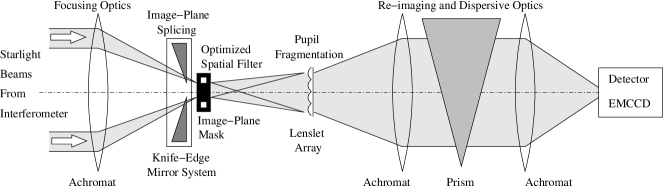
Figure 1: Schematic diagrom of the PAVO beam combiner at SUSI.

3.1 $\gamma$ Lupi

$\gamma$ Lupi (HR5776; Gam Lup) is a triple star system where its primary component ($\gamma$ Lupi A) is itself a suspected spectroscopic binary[19, 20] ($\gamma$ Lupi Aa-Ab). Its primary and secondary components ($\gamma$ Lupi A-B) form a visual binary. Table 2 shows the successful observations of $\gamma$ Lupi A-B carried out with PAVO and the calibrator stars used for the data analysis.

Table 2: Successful observations of $\gamma$ Lupi A-B

Date	Baseline	Range of HAs (Hr)	Calibrators
100805	N3-S1	0.99 – 1.50	HR4205, Tet Lup
100806	N3-S1	1.02 – 1.35	13 Sco
100813	N3-S3	0.74 – 1.02	Alf Tel
130705	N4-S2	0.60 – 1.20	Bet Lup, Del Lup
N3-S1=15m, N3-S3=40, N4-S2=60m

The full description of the data reduction pipeline from PAVO interferograms to calibrated $V^{2}$ data is beyond the scope of this paper. The pipeline is similar to the one used for reducing interferograms of the PAVO at CHARA beam combiner[21].

Each set of calibrated $V^{2}$ data (one set per successful observation) was used to fit a binary star model (see Eq. (2)) and to extract the relative astrometry of the binary star. The relative astrometry of a binary star is expressed in a polar coordinate system where the radial axis, $\rho$, measures the angular separation between the secondary and the primary component while the position angle axis, $\theta$, measures the bearing of the secondary component with respect to the celestial North. The 2D plane which the coordinate system defines is tangential to the celestial sphere. The relation between $\rho$ and $\theta$ with the equatorial coordinate system is,

$$\Delta\alpha=\rho\sin\theta,\quad\Delta\delta=\rho\cos\theta,$$ (3)

where $\Delta\alpha$ and $\Delta\delta$ are the small angle approximation of relative astrometry in the right ascension and declination axes respectively.

Comparisons between the two-dimensional $V^{2}$ data and the fitted model are shown in Fig. 2–3 in the form of grayscale images. The grayscale level represents the relative amplitude of $V^{2}$ in a given image. A fringe crossover event was successfully observed in The last image in Fig. 3 shows the climax of a fringe crossover event at HA$\sim$0.8 when the $V^{2}$ modulation stripe pattern is perpendicular to the HA axis. Despite missing the climax, the fringe crossover event was still in progress in all the other images. Also shown in the figures are cross-sectional plots of $V^{2}$ versus wavenumber at different hour angles. In the model fitting, the parameter $V^{2}_{1}$ was allowed to vary but $V^{2}_{2}$ was kept at 1 because the primary component of the binary is suspected to have a spectroscopic companion which may reduce fringe visibility while the secondary is estimated to be unresolved (UD$\lesssim$0.5mas). The accuracy of the values of $\beta$, $V^{2}_{1}$ and $V^{2}_{2}$ are less important as far as astrometry is concerned because the sinusoidal component of the visibility modulation depends only on the term $\phi$ in Eq. (1) which is related to the fringe packet separation of the primary and secondary components of the binary. Furthermore, the values of the 3 parameters are sensitive to how well the $V^{2}$ data are calibrated.

One drawback of this approach to determine the fringe packet separation indirectly from the modulation of the square of the fringe visibility is that the estimated position angle has a 180^∘ ambiguity. This ambiguity arises because the position of individual fringe packets could not be determined from the visibility modulation. Therefore the position angle extracted from the model fit could either be 96^∘ or 276^∘, if without any prior knowledge. In the case of $\gamma$ Lupi, the ambiguity is resolved by cross checking the values obtained with other techniques (e.g. speckle interferometry[22]).

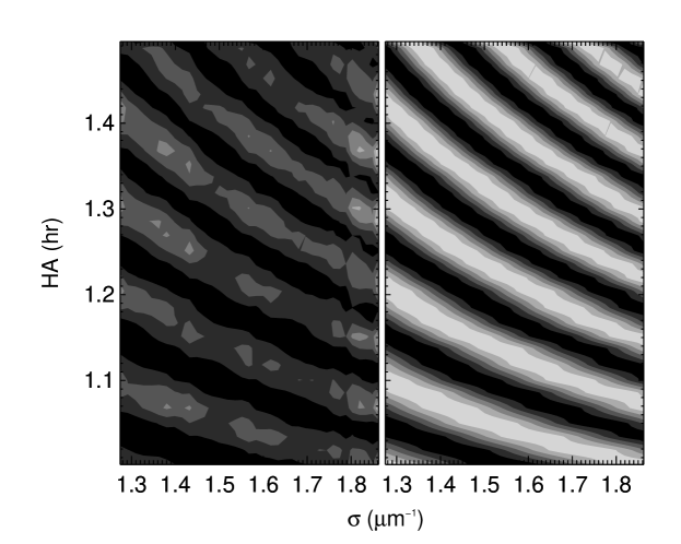
(a)

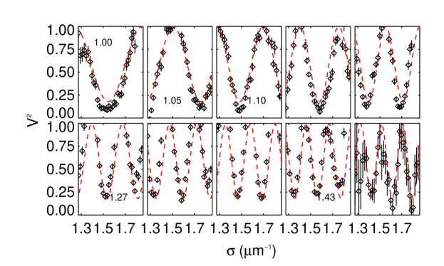
(b)

Figure 2: Calibrated $V^{2}$ (left panel of (a)) of $\gamma$ Lupi A-B obtained with PAVO on 5th August 2010 and the best fit binary star model (right panel of (a)). The grayscale in the images in (a) represents the relative amplitude of $V^{2}$ within each image. The difference in contrast between the data and model does not represent a discrepancy. Cross-sections of (a) at different hour angles (indicated in the legend) are plotted in (b) as $V^{2}$ versus wavenumber with the best fit model represented by the dashed lines.

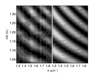
(a)

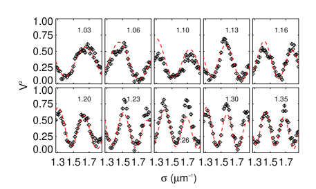
(b)

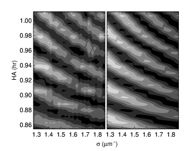
(c)

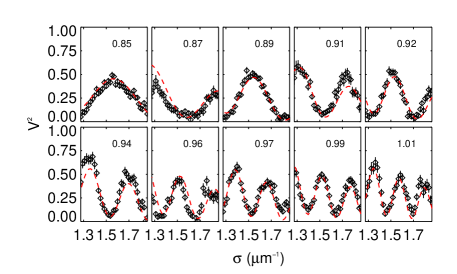
(d)

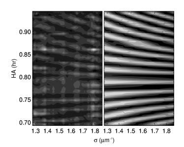
(e)

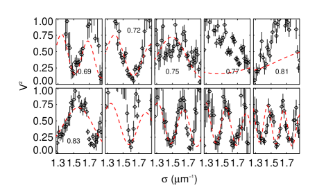
(f)

Figure 3: Similar to Fig. 2 but with data taken on 6th & 13th August 2010 and 5th July 2013 for plots on each row from top to bottom.

Table 3 shows the parameters extracted from the model-fitting as well as the number of $V^{2}$ data used and the reduced $\chi^{2}$ of the each fit. The values of reduced $\chi^{2}$ are larger than unity because a binary model is used in the model-fitting despite the primary component having a suspected spectroscopic companion. The discrepancy between the model and data is most obvious (see Fig. 3 when HA$\approx$0.79) at a time close to the instance when the fringe packets cross over because the modulation of the fringe visibility is dominated by the astrophysical feature of the primary component. Nevertheless, the astrometry of the wider pair ($\gamma$ Lupi A-B) based on the fitting of the sinusoidal component of the $V^{2}$ model is still good. The uncertainty numbers in the table are not scaled with $\sqrt{\chi^{2}_{R}}$ and do not contain systematic errors which are discussed in the next paragraph.

Table 3: Relative astrometry of $\gamma$ Lupi A-B

Parameter	2010.5925	2010.5952	2010.6143	2013.5078
$N_{V^{2}}$	37$\times$31	37$\times$20	37$\times$31	37$\times$142
LSTX (Hr)	16.371	16.376	16.378	16.374
$\beta_{\rm{A,B}}$	0.408$\pm$0.001	0.312$\pm$0.001	0.304$\pm$0.003	0.303$\pm$0.004
$\Delta\alpha_{\rm{A,B}}$ (mas)	-798.40$\pm$0.26	-803.64$\pm$0.29	-805.06$\pm$0.59	-811.81$\pm$0.31
$\Delta\delta_{\rm{A,B}}$ (mas)	84.76$\pm$0.04	85.82$\pm$0.05	85.86$\pm$0.07	86.05$\pm$0.03
$\rho_{\rm{A,B}}$ (mas)	802.9$\pm$0.3	808.2$\pm$0.3	809.6$\pm$0.6	816.4$\pm$0.3
$\theta_{\rm{A,B}}$ (∘)	276.05996$\pm$0.00002	276.09546$\pm$0.00003	276.08760$\pm$0.00008	276.05063$\pm$0.00001
$\chi^{2}_{\rm{R}}$	32.0	43.5	4.4	9.1
Systematic errors are not included in the uncertainties.

Table 4 shows the same extracted parameters but expressed in an equinox 2000 equatorial coordinate system. Also given in the table are astrometry from other techniques (mainly speckle interferometry) for comparison. The values reported in Ref. 22 in a series of papers given in the table have systematic errors of $\lesssim$0.5% in binary separation and $\sim$2^∘ in position angle[23]. Similarly, due to uncertainties in the baseline solutions and the wavelength scale used in the data reduction, the binary separation and position angle measurements obtained with PAVO may have systematic errors not reflected in the uncertainty numbers reported in the table. For most of the PAVO observations, instead of using a more precise approach [6], optical alignment was carried out with the standard SUSI alignment procedure. The latter approach typically aligns the apertures of the PAVO 2-hole mask with the pivot points of the siderostats to within 2cm. Assuming this offset is parallel to the $uv$-plane centered on the primary component of the binary star (the worst case), this translates to a systematic error of $<$0.08^∘ (upper limit set by the shortest 15m baseline) in the position angle measurements. An uncertainty in the baseline solution also translates to an uncertainty in the binary separation but the magnitude is smaller than the effect of an uncertainty in the wavelength scale. The estimated relative uncertainty in the wavelength scale is $\sim$1% ($\sim$6nm over $\sim$0.6$\mu$m). This estimation is based on the pixel offset value obtained during the PAVO wavelength scale calibration, which is typically $\lesssim$1 pixel or half of the width of one spectral channel. Since the relative uncertainty in wavelength scale directly translates to an uncertainty in the projected fringe packet separation measurement the systematic error in the binary separation measurements for $\gamma$ Lupi A-B is $\sim$8mas ($\sim$1% of $\sim$0.8^′′). Therefore the measurements obtained with PAVO are consistent with the values obtained with speckle interferometry[22, 24, 23]. The relative astrometry of the binary from various sources and the best fitted orbit are plotted in Fig. 4 for comparison.

Table 4: Comparison of $\gamma$ Lupi A-B astrometry.

Source	Julian yr.	$\theta$	$\delta\theta$	$\rho$	$\delta\rho$
	(+2000)	(∘)	(∘)	(′′)	(mas)
TOK2010†	09.2603y	275.7	0.0	0.8107	0.1
	09.2603H	275.8	0.1	0.8125	0.3
This work∗∗	10.5925	276.01	0.00	0.8033	0.3
	10.5952	276.05	0.00	0.8086	0.3
	10.6143	276.04	0.00	0.8101	0.6
	13.5078	275.99	0.00	0.8170	0.3
HAR2012#	11.3028y	275.5	0.2	0.8199	0.2
	11.3028I	275.5	0.0	0.8197	0.0
TOK2012‡	12.1845y	275.7	0.0	0.8242	0.1
Ephemeris∗	13.5000	276.7	–	0.8271	–
†Ref. 22
∗∗see Table 3 for $\delta\theta$
#Ref. 23
‡Ref. 24
∗based on a grade 3 orbit from Ref. 25
ymeasured at $\sim$550nm wavelength
Hmeasured at H$\alpha$ ($\sim$650nm) wavelength
Imeasured at $\sim$770nm wavelength

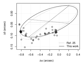
(a)

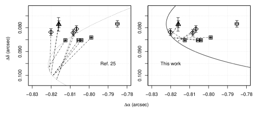
(b)

Figure 4: The relative positions of $\gamma$ Lupi A-B. The circular ($\bigcirc$) points are data obtained from the WDS (1835–1988) catalog and the Fourth Catalog of Interferometric Measurements of Binary Stars (1933–2006); the diamond ($\Diamond$) points are from Ref. 22 and Ref. 24; the triangular ($\triangle$) points are from Ref. 23; and the square ($\Box$) points are from this work. The ellipses in (a) and partially in (b) describe the orbit of the secondary component around the primary, which is centered at the origin in the plots. The orbital elements for the dotted elliptical lines are obtained from Ref. 25 while the solid elliptical lines are refitted with the available data. The period, $P$ ($=190$), the epoch of periastron, $T$ ($=1885.0$), and the eccentricity, $e$ ($=0.51$), of the orbit were kept the same. The updated values for the semimajor axis, $a$, the longitude of periastron, $\omega$, the longitude of ascending node, $\Omega$, and the inclination, $i$, of the orbit are 0.659^′′, 310.4^∘, 93.2^∘ and 95.3^∘ respectively.

3.2 $\zeta$ Sagittarii

$\zeta$ Sagittarii (HR7194; Zet Sgr) is a close binary star system which has an expected on-sky separation of 0.5^′′, a position angle of 265^∘ and an orbital period of 21 years[26]. The primary component ($\zeta$ Sagittarii A) is suspected to have an unresolved companion based on a discrepancy between the observed dynamical mass of the binary and its theoretical mass estimated from mass-magnitude relation[26].

Table 5 shows the number of observations attempted on this binary system. Despite being unsuccessful, the observation in 2012 hinted at the presence of a tertiary component because the PAVO $V^{2}$ data did not show any modulation and the fringe visibility was low, even with a short baseline. A successful follow up observation in 2013 resolved the tertiary component ($\zeta$ Sagittarii Ab).

Table 5: Successful and failed observations of $\zeta$ Sagittarii

Date	Baseline	Outcome	Range of HAs (Hr)	Calibrators
121003	N3-S1	Fail	2.5 – 3.5	Phi Sgr
130726	N4-S2	Success	-1.0 – -0.3	Phi Sgr
N3-S1=15m, N4-S2=60m

Fig. 5 shows the calibrated $V^{2}$ data obtained from the observation and the model that best fits the data. The high frequency modulation is contributed by the primary-secondary ($\zeta$ Sagittarii Aa-B) pair while the low frequency modulation (almost perpendicular to the former) is contributed by the primary-tertiary ($\zeta$ Sagittarii Aa-Ab) pair. The $V^{2}$ model of a triplet[11] used to fit the data is,

$$\begin{split}V_{1,2,3}^{2}=\frac{1}{\left(1+\beta_{2}+\beta_{3}\right)^{2}}\left\{\begin{array}[]{l}V_{1}^{2}+V_{2}^{2}\beta_{2}^{2}+V_{3}^{2}\beta_{3}^{2}\vspace{0.5em}\\ +2\sqrt{V_{1}^{2}V_{2}^{2}}\,\beta_{2}\cos\phi_{1,2}+2\sqrt{V_{1}^{2}V_{3}^{2}}\,\beta_{3}\cos\phi_{1,3}\vspace{0.5em}\\ +2\sqrt{V_{2}^{2}V_{3}^{2}}\,\beta_{2}\beta_{3}\cos(\phi_{1,2}-\phi_{1,3})\\ \end{array}\right\}\end{split},$$ (4)

where $V_{i}^{2}$ are the visibility squared of the fringes of the individual component stars, $\beta_{i}$ is the brightness ratio of the secondary or the tertiary component with respect to the primary, and,

$$\begin{split}\phi_{1,2}&=2\pi\sigma\Delta\vec{s}_{1,2}\cdot\vec{B},\\ \phi_{1,3}&=2\pi\sigma\Delta\vec{s}_{1,3}\cdot\vec{B}.\\ \end{split}$$ (5)

The subscript of $\Delta\vec{s}$ represents the pair of component stars the vector is related to. The remaining symbols in the equation were defined earlier. The astrometric parameters extracted from the model-fitting are listed in Table 6. In the model-fitting, all component stars were assumed to have angular diameters of $\sim$0.5mas (uniform form disk model). The number was obtained from the discrepancy in the total mass of the system[26] and their Hipparcos distance[27]. Since such diameters are unresolved on a 60m baseline, the parameters $V^{2}_{1}$, $V^{2}_{2}$ and $V^{2}_{3}$ were set to $\sim$1 at all wavelengths. The uncertainties of the parameters in Table 6 are not scaled with $\sqrt{\chi^{2}_{R}}$ and do not contain systematic errors. The table also includes relative astrometry from published work and ephemeris of the wider component pair for comparison. Although the statistical uncertainties of the parameters shown in the table are small, the true astrometric precision is limited by the systematic errors discussed in previous section. The estimated systematic errors in binary separation measurements are $\sim$5mas ($\sim$1% of $\sim$0.5^′′) for the Aa-B pair and $\sim$0.08mas ($\sim$1% of $\sim$0.008^′′) for the Aa-Ab pair. The estimated systematic error in position angle measurements is $\sim$0.02^∘ (the angle subtended by $\sim$2cm at a distance of 60m).

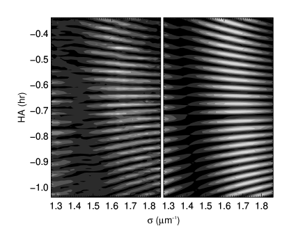
(a)

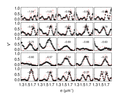
(b)

Figure 5: Calibrated $V^{2}$ (left panel of (a)) of $\zeta$ Sagittarii obtained with PAVO on 26th July 2013 and the best fitted ternary star model (right panel of (a)). The grayscale in the images in (a) represents the amplitude of $V^{2}$. The high and low frequency modulations are associated with the Aa-B and Aa-Ab component pairs respectively. Cross-sections of (a) at different hour angles are plotted in (b) as $V^{2}$ versus wavenumber with the best fitted model represented by the dashed lines. Discrepancy between the best fitted model and the data as seen in some of the panels in (b) suggests additional astrophysical structures (e.g. different spectral type) which are not included in the triplet model.

Table 6: Relative astrometry of $\zeta$ Sagittarii

Parameter	As fitted	Eq=J2000
Source	This work	This work	Ephemeris∗	DRS2012$\dagger$
Julian yr.	2013.5654	2013.5654	2013.5	2011.31
$N_{V^{2}}$	37$\times$126	–	–	–
LSTX (Hr)	18.396	–	–	–
$\beta_{\rm{Aa,B}}$	0.847$\pm$0.002	–	–	–
$\beta_{\rm{Aa,Ab}}$	0.778$\pm$0.002	–	–	–
$\Delta\alpha_{\rm{Aa,B}}$ (mas)	-501.36$\pm$0.02	-501.20$\pm$0.02	–	–
$\Delta\delta_{\rm{Aa,B}}$ (mas)	-42.610$\pm$0.002	-43.213$\pm$0.002	–	–
$\Delta\alpha_{\rm{Aa,Ab}}$ (mas)	4.11$\pm$0.02	4.10$\pm$0.02	–	–
$\Delta\delta_{\rm{Aa,Ab}}$ (mas)	6.537$\pm$0.002	6.542$\pm$0.002	–	–
$\rho_{\rm{Aa,B}}$ (mas)	503.17$\pm$0.02	503.06$\pm$0.02	500	304$\pm$4
$\theta_{\rm{Aa,B}}$ (∘)	265.142172$\pm$0.000001	265.072197$\pm$0.000001	265	285.59$\pm$0.17
$\rho_{\rm{Aa,Ab}}$ (mas)	7.72$\pm$0.01	7.72$\pm$0.01	–	–
$\theta_{\rm{Aa,Ab}}$ (∘)	32.158757$\pm$0.000005	32.076181$\pm$0.000005	–	–
$\chi^{2}_{\rm{R}}$	57.8	–	–	–
Systematic errors are not included in the uncertainties.
∗based on a grade 1 orbit from Ref. 26
†Ref. 26

4 Discussions

4.1 Astrometric error budget

The data analysis and results demonstrate the fringe packet crossover observation technique in performing precision astrometry on close binary stars. A summary of systematic errors that affect the accuracy of the results is listed in Table 7. The errors are listed according to two orthogonal axes in which they affect the measurements, i.e. along the binary separation axis, $\delta\rho$, and along the position angle axis, $\rho\delta\theta$. The dominant source of error in the $\rho$ axis is the accuracy of the wavelength scale while the dominant source of error in the $\theta$ axis is the misalignment between the imaging and the wide-angle baselines of the interferometer (see Ref 28 for definitions). As a result, the astrometric error in the right ascension and declination axes varies between the limits set by the two dominant error sources as a function of $\theta$.

Errors arising from anisoplanatism of the turbulent atmosphere and time-stamping of observation data is negligible. The former is derived with an atmospheric coefficient[29] of $\sim$780 m^2/3s^1/2arcsec^-1 for a total integration time of at least 10 minutes while the latter is derived from the accuracy of the system clock of the computer used for observation. Lastly, the contribution of the uncertainty in measuring the fringe visibility to the astrometric error is mainly from its random error component. The astrometric error is not sensitive to a bias in the $V^{2}$ measurement because the astrometric parameters extracted from the model-fitting are dependent on the frequency of the $V^{2}$ modulation. The bias, if it exists, is assumed to be introduced by the data reduction algorithm and is wavelength and time invariant. On the other hand, the random error of the $V^{2}$ measurement (usually expressed in terms of SNR) directly affects the astrometric error through the model-fitting process. Although it is intuitive that a lower SNR produces a larger astrometric error, it is difficult to derive an analytical solution to relate the two errors. Therefore, for the sake of comparison with other sources of error, the magnitude of the astrometric error due to the random $V^{2}$ error is estimated from the results in the previous section. The calibrated $V^{2}$ measurements have a range of average SNR between 5 to 25.

Table 7: Breakdown of astrometric error

Source of errors	$\delta\rho$	$\rho\delta\theta$
	($\mu$as)	($\mu$as)
dOPD-related
Anisoplanatism	$<$10	$<$10
Biases in $V^{2}$ measurements	–	–
Random errors in $V^{2}$ measurements	$<$400	$\lesssim$1
Wavelength scale of spectrograph	10$\times 10^{3}$	–
Timing accuracy	$<$2	$<$2
Baseline-related
Wide-angle baseline solution	2	2
Imaging baseline alignment∗	200	200
Combined error	$\sim$10$\times 10^{3}$	$\sim$200
Estimated errors assumed:
(a) binary separation is 1′′
(b) baseline is 100m
∗$>$20$\times$ smaller with the MUSCA alignment

4.2 Next-generation instrument

The error budget in Table 7 shows two limiting factors for the indirect approach method to reach higher astrometric precision. In view of this, this subsection discusses possible improvements to the PAVO beam combiner so that the astrometric errors determined by the two limiting factors can be reduced. In addition, a next-generation instrument incorporating the suggested improvements is also discussed.

Firstly, the uncertainty of the wavelength scale can be reduced by increasing the spectral resolution of the PAVO spectrograph and by adopting a more precise wavelength calibration procedures. With the same spectral bandwidth, $\Delta\sigma$, an increase in spectral resolution by a factor of 100 reduces the astrometric error by a similar factor because,

$$\frac{\delta\rho}{\rho}\propto\frac{\delta\text{dOPD}}{\text{dOPD}}\propto\frac{\delta\sigma}{\sigma}\propto\frac{1}{R},$$ (6)

where $R$ denotes the resolving power of the spectrograph. Note that a high resolution spectrum in near infrared (IR) wavelengths is less desirable because $\Delta\sigma$ in the common $J$, $H$ and $K$ bands (0.19$\mu$m^-1, 0.11$\mu$m^-1 and 0.08$\mu$m^-1 respectively) is much smaller than in the visible wavelengths. Even with all the near IR bands combined, the spectral bandwidth is only half that of PAVO’s. This affects the number of $V^{2}$ modulation cycles seen across the bandwidth for a given dOPD. A smaller number of cycles yields a larger astrometric error from the model-fitting process. An example of a high resolution spectro-interferometric instrument is the VEGA beam combiner at CHARA which has a spectral resolving power of 30000 and operates in the visible wavelengths[30].

The reduction in wavelength uncertainty with this approach comes at a cost of reduced flux per spectral channel or more critically an increase in the fringe visibility uncertainty. In the photon noise limited regime,

$$\frac{\delta V^{2}}{V^{2}}=\frac{1}{\text{SNR}}\propto\sqrt{R}\propto\frac{1}{D_{\text{tel}}\sqrt{T_{\text{exp}}}},$$ (7)

while in the detector noise regime (when observing faint targets), $\delta V^{2}/V^{2}\propto R$. Such a cost can be partially offset by the exceptional seeing condition in Antarctica, where this observation technique is most efficient. With an atmospheric coherence time of more than 8$\times$ that at SUSI (see Table 8), the exposure time, $T_{\text{exp}}$, of one frame of interferogram can be $\sim$10$\times$ as long in Antarctica. The additional factor of $\sqrt{10}$ can be offset by using siderostats with a larger diameter. Therefore, the next generation instrument should be used with siderostats of about 60cm in diameter, $D_{\text{tel}}$, a size similar to those used at the Palomar Testbed Interferometer (PTI) and the Navy Precision Optical Interferometer (NPOI).

Another advantage of having a high-resolution spectrograph is the long coherence length of the dispersed fringes. Since the standard deviation of fringe motion due to atmospheric turbulence is expected to be $\lesssim$50$\lambda$ in Antarctica, the dispersed fringes will always ($\sim 99.7\%$ of the time) be visible to the beam combining instrument even at a low tracking rate ($\sim$20Hz) if the spectral resolution of the spectrograph is larger than 300.

Secondly, the uncertainty of the baseline alignment can be reduced by adopting a more precise optical alignment procedure. A procedure developed for a dedicated astrometric beam combiner, MUSCA, at SUSI[6] can align the pivot point of two siderostat pupils at the beam combiner to an uncertainty of $\sim$1mm. The pivot point of a siderostat (or a telescope) is defined as the intersection point between two of its axes of motion, i.e. altitude and azimuth. In the case of a siderostat, this point coincides with the center of the circular aperture of the mirror. The separation of the pivot points of a pair of siderostats (or telescopes) fundamentally defines the wide-angle baseline of an interferometer. The pivot point of a good siderostat can be kept from deviating from the center of the circular aperture to less than 100$\mu$m within a time-scale of the order of a few weeks[31, 32]. The amount of deviation can be characterized and is included as part of the baseline uncertainty for the astrometric measurement. In addition, an IR LED can be inserted into a hole centered on a siderostat, a design similar to an astrometric siderostat of NPOI[33], for real time monitoring of the deviation if necessary.

The anisoplanatism of the turbulent atmosphere would be come the limiting factor for higher precision astrometry once the wavelength scale calibration and the imaging baseline alignment issues are addressed. Table 8 shows the comparison of atmospheric conditions between 3 different astronomical sites. The atmosphere in Antarctica is estimated to have $\sim$3$\times$ larger turbulent cells (indicated by the Fried parameter, $r_{0}$) than the atmosphere above SUSI. Having such a stable atmosphere, the systematic astrometric error due to anisoplanatism (which is inversely proportional to $r_{0}^{5/6}$) is negligible in Antarctica. Consequently, an hour long observation at SUSI would require $\sim$5 minutes (a factor of $\sim$3² shorter in time) with the same instrument to produce the same level of astrometric accuracy in Antarctica.

Table 8: Typical/median atmospheric conditions^† at various long baseline interferometers

Parameter	SUSI	VLTI	Dome C#,∗
Seeing (′′)	1.3	0.86	0.23
$r_{0}$ (cm)	7.1	11	26
$\tau_{0}$ (ms-1)	1	3.9	8.6
$L_{0}$ (m)	$<$80	22	$\sim$8
References	Ref. 34, 35, 36	Ref. 37, 38	Ref. 39, 40
†specified at 500nm wavelength
#site used as a proxy for an interferometer in Antarctica
∗assumed siderostats/telescopes are elevated ($\gtrsim$30m above ground)

Table 9 lists the features to be implemented for the next generation instrument, which include the several upgrades discussed above. Two additional desirable features are an extra baseline and a wider field of view. An extra baseline, $B_{2}$, independent and orthogonal to the first, $B_{1}$, can reduce the astrometric uncertainty by a factor of $\sqrt{1+(B_{2}/B_{1})^{4/3}}$ in the direction of the binary separation when used simultaneously during the fringe crossover event observation. However, the main motivation to include an additional baseline, especially a shorter one, is to make observable those stars which would have A wider field of view increases the number of observable targets. Although it does not increase the number significantly, it would allow $\alpha$ Cen A-B, the closest star system to Earth and suspected to harbor a near Earth-size planet [41], to be observed. The binary separation will remain within 5^′′ for the next 5 years[42]. The next epoch when the binary separation is expected to be $<$5^′′ again is during the periastron of the secondary component in 2035. Follow-up astrometric observations of the binary would give a constraint on the mass of the suspected planet and the presence of other planets further away from the host star. The additional shorter baseline would be necessary for such observations.

Table 9: Proposed features of an Antarctic instrument for narrow-angle astrometry

Parameter	Details/specifications
Facility related
Baselines	2, independent and orthogonal
	1$\times$ 10m, 1$\times$ 100m
Baseline alignment	Similar to the scheme for MUSCA at SUSI
Light collecting elements	4$\times$ 60cm-diameter siderostats
Field of view	$<$5′′
Beam combiner related
Optical design	Similar to PAVO
Spectral bandwidth, $\Delta\sigma$	0.5–0.8$\mu$m (V band∗)
Spectral resolution, $R$	$\sim$5000 (100$\times$ PAVO)
Number of channels, $N_{\text{ch}}$	$\sim$2100 (100$\times$ PAVO)
Coherence length per channel, $L_{\text{coh}}$	$\sim$3mm
∗see Sec. 4 for discussion on using NIR bands

5 Conclusions

Based on the results from prototype observations with SUSI and the proposed enhancements for a next generation instrument, the indirect approach to narrow-angle astrometry method is capable of achieving accuracy in the regime of tens of micro-arcseconds. This method does not require an additional metrology system for path length measurement and uses a straightforward beam combining instrument with no moving mechanical parts. Only the main delay line and the siderostats, which are the essential parts of an optical long baseline interferometer, have moving parts and therefore may require regular maintenance. This makes the method very suitable to be deployed at a remote and poorly accessible observation site like Antarctica.

- [1] Shao, M. and Colavita, M., “Potential of long-baseline infrared interferometry for narrow-angle astrometry,” A&A 262, 353–358 (1992).
- [2] Muterspaugh, M. W., Lane, B. F., Kulkarni, S. R., Konacki, M., Burke, B. F., Colavita, M. M., Shao, M., Wiktorowicz, S. J., and O’Connell, J., “The Phases Differential Astrometry Data Archive. I. Measurements and Description,” AJ 140, 1579–1622 (Dec. 2010).
- [3] Delplancke, F., “The PRIMA facility phase-referenced imaging and micro-arcsecond astrometry,” New Astronomy Review 52, 199–207 (June 2008).
- [4] Bartko, H., Perrin, G., Brandner, W., Straubmeier, C., Richichi, A., Gillessen, S., Paumard, T., Hippler, S., Eckart, A., Schöller, M., Eisenhauer, F., Haubois, X., Lenzen, R., Rabien, S., Clénet, Y., Ramos, J. R., Thiel, M., Berger, J. P., Baumeister, H., Kellner, S., Cassaing, F., Böhm, A., Hofmann, R., Gendron, E., Klein, R., Dodds-Eden, K., Houairi, K., Hormuth, F., Gräter, A., Kervella, P., Naranjo, V., Genzel, R., Fédou, P., Henning, T., Hamaus, N., Jocou, L., Neumann, U., Haug, M., Lacour, S., Laun, W., Kolmeder, J., Malbet, F., Rohloff, R., Pfuhl, O., Perraut, K., Ziegleder, J., Rouan, D., Rousset, G., Amorim, A., and Lima, J., “GRAVITY: Astrometry on the galactic center and beyond,” New A Rev. 53, 301–306 (Nov. 2009).
- [5] Pott, J., Woillez, J., Akeson, R. L., Berkey, B., Colavita, M. M., Cooper, A., Eisner, J. A., Ghez, A. M., Graham, J. R., Hillenbrand, L., Hrynewych, M., Medeiros, D., Millan-Gabet, R., Monnier, J., Morrison, D., Panteleeva, T., Quataert, E., Randolph, B., Smith, B., Summers, K., Tsubota, K., Tyau, C., Weinberg, N., Wetherell, E., and Wizinowich, P. L., “Astrometry with the Keck Interferometer: The ASTRA project and its science,” New A Rev. 53, 363–372 (Nov. 2009).
- [6] Kok, Y., Ireland, M. J., Tuthill, P. G., Robertson, J. G., Warrington, B. A., Rizzuto, A. C., and Tango, W. J., “Phase-Referenced Interferometry and Narrow-Angle Astrometry with SUSI,” JAI 2, 40011 (Dec. 2013).
- [7] Schuhler, N., Salvadé, Y., Lévêque, S., Dändliker, R., and Holzwarth, R., “Frequency-comb-referenced two-wavelength source for absolute distance measurement,” Optics Letters 31, 3101–3103 (Nov. 2006).
- [8] Gillessen, S., Lippa, M., Eisenhauer, F., Pfuhl, O., Haug, M., Kellner, S., Ott, T., Wieprecht, E., Sturm, E., Haußmann, F., Kister, C. F., Moch, D., and Thiel, M., “GRAVITY: metrology,” in [Proc. SPIE ], 8445 (July 2012).
- [9] Kok, Y., Ireland, M. J., Robertson, J. G., Tuthill, P. G., Warrington, B. A., and Tango, W. J., “Low-cost scheme for high-precision dual-wavelength laser metrology,” Appl. Opt. 52, 2808–2814 (April 2013).
- [10] Tuthill, P. G., “Optical interferometry from the antarctic,” in [Proc. IAU Symp. Astrophysics from Antarctica ], (288) (2012).
- [11] Tango, W. J., “The determination of the orbital elements of binary stars (Internal SUSI report),” The University of Sydney (July 2006).
- [12] Armstrong, J. T., Clark, III, J. H., Gilbreath, G. C., Hindsley, R. B., Hutter, D. J., Mozurkewich, D., and Pauls, T. A., “Precision narrow-angle astrometry of binary stars with the Navy Prototype Optical Interferometer,” in [Proc. SPIE ], 5491, 1700–1706 (Oct. 2004).
- [13] Davis, J., Mendez, A., Seneta, E. B., Tango, W. J., Booth, A. J., O’Byrne, J. W., Thorvaldson, E. D., Ausseloos, M., Aerts, C., and Uytterhoeven, K., “Orbital parameters, masses and distance to Centauri determined with the Sydney University Stellar Interferometer and high-resolution spectroscopy,” MNRAS 356, 1362–1370 (Feb. 2005).
- [14] Tango, W. J., Davis, J., Jacob, A. P., Mendez, A., North, J. R., O’Byrne, J. W., Seneta, E. B., and Tuthill, P. G., “A new determination of the orbit and masses of the Be binary system Scorpii,” MNRAS 396, 842–848 (June 2009).
- [15] Monnier, J. D., Berger, J.-P., Millan-Gabet, R., and ten Brummelaar, T. A., “The Michigan Infrared Combiner (MIRC): IR imaging with the CHARA Array,” in [New Frontiers in Stellar Interferometry ], Traub, W. A., ed., Society of Photo-Optical Instrumentation Engineers (SPIE) Conference Series 5491, 1370 (Oct. 2004).
- [16] Petrov, R. G., Malbet, F., Weigelt, G., Antonelli, P., Beckmann, U., Bresson, Y., Chelli, A., Dugué, M., Duvert, G., Gennari, S., Glück, L., Kern, P., Lagarde, S., Le Coarer, E., Lisi, F., Millour, F., Perraut, K., Puget, P., Rantakyrö, F., Robbe-Dubois, S., Roussel, A., Salinari, P., Tatulli, E., Zins, G., Accardo, M., Acke, B., Agabi, K., Altariba, E., Arezki, B., Aristidi, E., Baffa, C., Behrend, J., Blöcker, T., Bonhomme, S., Busoni, S., Cassaing, F., Clausse, J.-M., Colin, J., Connot, C., Delboulbé, A., Domiciano de Souza, A., Driebe, T., Feautrier, P., Ferruzzi, D., Forveille, T., Fossat, E., Foy, R., Fraix-Burnet, D., Gallardo, A., Giani, E., Gil, C., Glentzlin, A., Heiden, M., Heininger, M., Hernandez Utrera, O., Hofmann, K.-H., Kamm, D., Kiekebusch, M., Kraus, S., Le Contel, D., Le Contel, J.-M., Lesourd, T., Lopez, B., Lopez, M., Magnard, Y., Marconi, A., Mars, G., Martinot-Lagarde, G., Mathias, P., Mège, P., Monin, J.-L., Mouillet, D., Mourard, D., Nussbaum, E., Ohnaka, K., Pacheco, J., Perrier, C., Rabbia, Y., Rebattu, S., Reynaud, F., Richichi, A., Robini, A., Sacchettini, M., Schertl, D., Schöller, M., Solscheid, W., Spang, A., Stee, P., Stefanini, P., Tallon, M., Tallon-Bosc, I., Tasso, D., Testi, L., Vakili, F., von der Lühe, O., Valtier, J.-C., Vannier, M., and Ventura, N., “AMBER, the near-infrared spectro-interferometric three-telescope VLTI instrument,” A&A 464, 1–12 (Mar. 2007).
- [17] Ireland, M. J., Mérand, A., ten Brummelaar, T. A., Tuthill, P. G., Schaefer, G. H., Turner, N. H., Sturmann, J., Sturmann, L., and McAlister, H. A., “Sensitive visible interferometry with PAVO,” in [Proc. SPIE ], 7013 (July 2008).
- [18] Robertson, J. G., Ireland, M. J., Tango, W. J., Davis, J., Tuthill, P. G., Jacob, A. P., Kok, Y., and Ten Brummelaar, T. A., “Instrumental developments for the Sydney University Stellar Interferometer,” in [Proc. SPIE ], 7734 (July 2010).
- [19] Levato, H., Malaroda, S., Morrell, N., and Solivella, G., “Stellar multiplicity in the Scorpius-Centaurus association,” ApJS 64, 487–503 (June 1987).
- [20] Docobo, J. A. and Andrade, M., “A Methodology for the Description of Multiple Stellar Systems with Spectroscopic Subcomponents,” ApJ 652, 681–695 (Nov. 2006).
- [21] Maestro, V., Kok, Y., Huber, D., Ireland, M. J., Tuthill, P. G., White, T., Schaefer, G., ten Brummelaar, T. A., McAlister, H. A., Turner, N., Farrington, C. D., and Goldfinger, P. J., “Imaging rapid rotators with the PAVO beam combiner at CHARA,” in [Proc. SPIE ], 8445 (July 2012).
- [22] Tokovinin, A., Mason, B. D., and Hartkopf, W. I., “Speckle Interferometry at the Blanco and SOAR Telescopes in 2008 and 2009,” AJ 139, 743–756 (Feb. 2010).
- [23] Hartkopf, W. I., Tokovinin, A., and Mason, B. D., “Speckle Interferometry at SOAR in 2010 and 2011: Measures, Orbits, and Rectilinear Fits,” AJ 143, 42 (Feb. 2012).
- [24] Tokovinin, A., “Speckle Interferometry and Orbits of “Fast” Visual Binaries,” AJ 144, 56 (Aug. 2012).
- [25] Heintz, W. D., “Orbits of 15 visual binaries,” A&AS 82, 65–69 (Jan. 1990).
- [26] De Rosa, R. J., Patience, J., Vigan, A., Wilson, P. A., Schneider, A., McConnell, N. J., Wiktorowicz, S. J., Marois, C., Song, I., Macintosh, B., Graham, J. R., Bessell, M. S., Doyon, R., and Lai, O., “The Volume-limited A-Star (VAST) survey - II. Orbital motion monitoring of A-type star multiples,” MNRAS 422, 2765–2785 (June 2012).
- [27] van Leeuwen, F., “Validation of the new Hipparcos reduction,” A&A 474, 653–664 (Nov. 2007).
- [28] Woillez, J. and Lacour, S., “Wide-angle, Narrow-angle, and Imaging Baselines of Optical Long-baseline Interferometers,” ApJ 764, 109 (Feb. 2013).
- [29] Kok, Y., Phase-referencing interferometry and narrow-angle astrometry with SUSI, PhD thesis, The University of Sydney (2014).
- [30] Mourard, D., Clausse, J. M., Marcotto, A., Perraut, K., Tallon-Bosc, I., Bério, P., Blazit, A., Bonneau, D., Bosio, S., Bresson, Y., Chesneau, O., Delaa, O., Hénault, F., Hughes, Y., Lagarde, S., Merlin, G., Roussel, A., Spang, A., Stee, P., Tallon, M., Antonelli, P., Foy, R., Kervella, P., Petrov, R., Thiebaut, E., Vakili, F., McAlister, H., ten Brummelaar, T., Sturmann, J., Sturmann, L., Turner, N., Farrington, C., and Goldfinger, P. J., “VEGA: Visible spEctroGraph and polArimeter for the CHARA array: principle and performance,” A&A 508, 1073–1083 (Dec. 2009).
- [31] Colavita, M., Wallace, J., Hines, B., Gursel, Y., Malbet, F., Palmer, D., Pan, X., Shao, M., Yu, J., Boden, A., and Others, “The Palomar testbed interferometer,” ApJ 510, 505–521 (1999).
- [32] Davis, J., Tango, W. J., Booth, A. J., Thorvaldson, E. D., and Giovannis, J., “The Sydney University Stellar Interferometer - II. Commissioning observations and results,” MNRAS 303, 783–791 (Mar. 1999).
- [33] Armstrong, J. T., Mozurkewich, D., Rickard, L. J., Hutter, D. J., Benson, J. A., Bowers, P. F., Elias, II, N. M., Hummel, C. A., Johnston, K. J., Buscher, D. F., Clark, III, J. H., Ha, L., Ling, L., White, N. M., and Simon, R. S., “The Navy Prototype Optical Interferometer,” ApJ 496, 550–571 (Mar. 1998).
- [34] ten Brummelaar, T., “Taking the Twinkle Out of the Stars: an Adaptive Wavefront Tilt Correction Servo and Preliminary Seeing Study for SUSI,” PASP 106, 915 (Aug. 1994).
- [35] Davis, J., Lawson, P. R., Booth, A. J., Tango, W. J., and Thorvaldson, E. D., “Atmospheric path variations for baselines up to 80m measured with the Sydney University Stellar Interferometer,” MNRAS 273, L53–L58 (Apr. 1995).
- [36] Davis, J. and Tango, W., “Measurement of the Atmospheric Coherence Time,” PASP 108, 456–+ (May 1996).
- [37] Sarazin, M. and Tokovinin, A., “The Statistics of Isoplanatic Angle and Adaptive Optics Time Constant derived from DIMM Data,” in [European Southern Observatory Conference and Workshop Proceedings ], Vernet, E., Ragazzoni, R., Esposito, S., and Hubin, N., eds., European Southern Observatory Conference and Workshop Proceedings 58, 321 (2002).
- [38] Martin, F., Conan, R., Tokovinin, A., Ziad, A., Trinquet, H., Borgnino, J., Agabi, A., and Sarazin, M., “Optical parameters relevant for High Angular Resolution at Paranal from GSM instrument and surface layer contribution,” A&AS 144, 39–44 (May 2000).
- [39] Agabi, A., Aristidi, E., Azouit, M., Fossat, E., Martin, F., Sadibekova, T., Vernin, J., and Ziad, A., “First Whole Atmosphere Nighttime Seeing Measurements at Dome C, Antarctica,” PASP 118, 344–348 (Feb. 2006).
- [40] Ziad, A., Aristidi, E., Agabi, A., Borgnino, J., Martin, F., and Fossat, E., “First statistics of the turbulence outer scale at Dome C,” A&A 491, 917–921 (Dec. 2008).
- [41] Dumusque, X., Pepe, F., Lovis, C., Ségransan, D., Sahlmann, J., Benz, W., Bouchy, F., Mayor, M., Queloz, D., Santos, N., and Udry, S., “An Earth-mass planet orbiting Centauri B,” Nature 491, 207–211 (Nov. 2012).
- [42] Pourbaix, D., Nidever, D., McCarthy, C., Butler, R. P., Tinney, C. G., Marcy, G. W., Jones, H. R. A., Penny, A. J., Carter, B. D., Bouchy, F., Pepe, F., Hearnshaw, J. B., Skuljan, J., Ramm, D., and Kent, D., “Constraining the difference in convective blueshift between the components of alpha Centauri with precise radial velocities,” A&A 386, 280–285 (Apr. 2002).