Spectral/hp element methods for plane Newtonian extrudate swell

Spectral/hp element methods for plane Newtonian extrudate swell

Spectral/hp element methods and an arbitrary Lagrangian-Eulerian (ALE) moving-boundary technique are used to investigate planar Newtonian extrudate swell. Newtonian extrudate swell arises when viscous liquids exit long die slits. The problem is characterised by a stress singularity at the end of the slit which is inherently difficult to capture and strongly influences the predicted swelling of the fluid. The impact of inertia ($0\leq\text{Re}\,\leq 100$) and slip along the die wall on the free surface profile and the velocity and pressure values in the domain and around the singularity are investigated. The high order method is shown to provide high resolution of the steep pressure profile at the singularity. The swelling ratio and exit pressure loss are compared with existing results in the literature and the ability of high-order methods to capture these values using significantly fewer degrees of freedom is demonstrated.

1 Introduction

In this article, we investigate the extrudate swell phenomenon, which is a radial swelling of free liquid jets exhibited by viscous fluids exiting long die slits. This jet swelling is particularly strong for viscoelastic fluids but is also exhibited by low Reynolds number Newtonian fluids. The prediction of the swelling ratio is very important in a range of industrial processes such as inkjet printing, extrusion moulding or cable coating.

The swelling of Newtonian jets is mainly characterised by the reorganisation of the velocity profile from the parabolic Poiseuille flow inside the die to plug flow downstream (Tanner (2002)). This transition is characterised by the sudden jump in the shear stress at the die exit (Russo (2009)). Inside the die, the shear stress at the wall is at its maximum with particles sticking to the wall (for the no-slip boundary condition). Then immediately after the die exit, the removal of the wall shear stress causes a boundary layer to form at the free surface. In this layer, the parabolic velocity profile adjusts itself so as to satisfy the condition of zero shear stress at the free surface. This sudden jump in the shear stress at the die exit causes an almost instantaneous acceleration of the particles at the free surface causing the fluid jet to swell.

Due to the presence of this stress singularity at the die exit, numerical simulations of the extrudate swell phenomenon are particularly challenging. Analytically, this singularity originates from the sudden change in the boundary condition from the wall of the die to the free surface of the exiting jet. This ”jump” in the boundary condition yields steep and infinite stress and pressure concentrations at the singular point. These infinite stress values near the singularity affect the accuracy of the numerical solution and the size of the swelling and therefore need to be resolved as accurately as possible. In this contribution, we use a spectral/$hp$ element method to improve our ability to capture these stress concentrations. Traditional discretisation methods such as finite differences or low-order finite elements require a very large number of degrees of freedom to resolve these sharp stress variations.

In this article, we will describe a spectral/$hp$ method that is capable of approximating the infinite stress values with an exponential increase in the extreme values of the pressure with $p$-refinement. This demonstrates that our high order method provides a high-quality approximation of the stress singularity with a very low number of degrees of freedom. We will give detailed information about the pressure and velocity in the vicinity of the singularity for a wide range of Reynolds numbers ($0\leq\text{Re}\,\leq 100$) and for slip along the die wall. We demonstrate that our method predicts swell ratios and exit pressure loss corrections in excellent agreement with a recent numerical study of Mitsoulis et al. (2012) for our coarsest approximation $P=10$. Mitsoulis et al. (2012) used a low order finite element method with a high mesh refinement around the singularity.

Typically, a decrease in the swelling is observed for an increase in the resolution of the singularity. In the existing literature, the stress values at the singularity are rarely addressed. Salamon et al. (1995) investigated the role of surface tension and slip on the singularity numerically and analytically. They demonstrated that a very fine mesh near the singularity is needed to predict the singular pressure and stress behaviour with sufficient accuracy. Georgiou and Boudouvis (1999) compared the singular finite element method with the regular finite element method for the extrudate swell problem. In the singular finite element method basis functions in the elements around the singularity are enriched with the local asymptotic solution for the singularity. They demonstrated that with this method the predictions of the swell ratio converged. However, the singular finite element method requires the correct asymptotic behaviour of the pressure at the corner singularity and the asymptotic solution for the pressure is obtained assuming Stokes-like behaviour around the singularity. This means this approach is only accurate for $\text{Re}\,=0$. Indeed, Georgiou and Boudouvis (1999) found that the singular finite element method was outperformed by the regular finite element method for extrudate swell including inertia. Our method is capable of resolving the stress singularity with spectral convergence properties without making any assumptions on the form of the singularity.

Inertialess extrudate planar Newtonian swell has been investigated in terms of swell ratios using low order finite elements by a wide range of authors (Tanner (1973), Nickell et al. (1974), Crochet and Keunings (1982), Reddy and Tanner (1978)). Tanner (2002) provides a review of inertialess Newtonian swell ratio results. Only very few investigations involved the use of higher order methods. Ho and Rønquist (1994) provided the first extrudate swell computation with a spectral method for one coarse mesh with $8$ spectral elements with polynomial order $4$ for $\text{Re}\,=0$. They predicted a swell ratio of $1.1840$. Russo (2009) used the spectral element method to predict free surface profiles and swell ratios for $0\leq\text{Re}\,\leq 10$ and surface tension for $4$ spectral elements with polynomial order $6<P<14$. We will use a spectral element mesh with $14$ spectral elements and $10\leq P\leq 16$ with a smaller element size around the singularity providing a much higher resolution there compared with previous studies. We will provide results for $0\leq\text{Re}\,\leq 100$ and for a slip condition along the die wall.

The paper is organised as follows. In Section 2, we will introduce the governing equations for the description of Newtonian free surface flow and the equations of motion for the mesh movement. We will conclude this Section with a description of the boundary conditions for the extrudate swell problem and the definition of the quantities of interest such as swelling ratio and exit pressure correction. In Section 3, we describe the numerical discretisation of the governing equations. In Section 4, we give numerical results for the impact of inertia and slip on the extrudate swell problem including detailed plots for velocity and pressure profiles in different parts of the domain.

2 Formulation

2.1 Governing Equations of the Fluid

The free surface motion of an incompressible fluid flow can be characterised by the incompressible Navier-Stokes equations describing the motion of the fluid and the motion of the free surface. On a moving domain $\Omega_{t}\subset\mathbb{R}^{d}$, $t\in I\equiv(t_{0},T)$, they can be expressed as

$$\text{Re}\,\left(\dfrac{\partial\mathbf{u}}{\partial t}+(\mathbf{u}\cdot\nabla)\mathbf{u}\right) =-\nabla p+2\,\nabla\cdot\mathbf{D} \mbox{in }\Omega_{t},t\in I,$$ (1a)

$$\nabla\cdot\mathbf{u} =0 \mbox{in }\Omega_{t},t\in I,$$ (1b)

$$\mathbf{u} =\mathbf{u}_{0} \mbox{in }\hat{\Omega}_{t_{0}},$$ (1c)

$$\mathbf{u} =\mathbf{u}_{D} \mbox{on }\partial\Omega_{t},t\in I,$$ (1d)

where $\mathbf{u}$ is the velocity, $p$ is the pressure, $\mathbf{D}=\frac{1}{2}(\nabla\mathbf{u}+\nabla\mathbf{u}^{T})$ is the rate of deformation tensor, Re  is the Reynolds number, $\mathbf{u}_{0}$ is the velocity field at $t=t_{0}$ and $\mathbf{u}_{D}$ is the assigned Dirichlet boundary condition.

The motion of the free surface, $\Gamma_{f}$, is characterised by the following boundary conditions

$$\mathbf{u}\cdot\mathbf{n} =\mathbf{w}\cdot\mathbf{n} \mbox{on }\Gamma_{f}\quad\mbox{ (kinematic)}$$ (2a)

$$\left[\boldsymbol{\sigma}\right]\cdot\mathbf{n} =\sigma\kappa\mathbf{n} \mbox{on }\Gamma_{f}\quad\mbox{ (dynamic)}$$ (2b)

where $\mathbf{w}$ is the velocity of the free surface, $\sigma$ is the surface tension coefficient, $\kappa$ is the curvature of the free surface, $\mathbf{n}$ is the unit outward normal to the free surface and $\left[\boldsymbol{\sigma}\right]$ denotes the jump in the Cauchy stress tensor across the free surface.

In order to track the free surface motion computationally, the grid points of our computational mesh at the free surface are moved with the normal fluid velocity, which ensures that particles do not cross the interface and therefore that the kinematic condition (2a) is satisfied.

To avoid mesh distortion, the mesh points in the interior of the domain are moved with an arbitrary speed. This use of arbitrary mesh movement is known as the arbitrary Lagrangian-Eulerian (ALE) technique. The ALE formulation relates the Navier-Stokes equations on the moving domain (1) to a formulation on a referential configuration $\hat{\Omega}_{t_{0}}$. At each $t\in I$, each point of the reference configuration $\mathbf{Y}$ is then associated to a point $\boldsymbol{x}$ in the current domain $\Omega_{t}$ using the so-called ALE-map (Donea et al., 2004; Scovazzi and Hughes, 2007; Pena, 2009; Nobile, 2001), that is,

$$\mathcal{R}_{t}:\hat{\Omega}_{t_{0}}\rightarrow \Omega_{t}, \forall t\geq 0,$$

$$\mathbf{Y}\mapsto \boldsymbol{x}(\mathbf{Y},t)=\mathcal{R}_{t}(\mathbf{Y}), \forall\mathbf{\mathbf{Y}}\in\hat{\Omega}_{t_{0}},$$ (3)

where $\mathbf{Y}$ is called the ALE coordinate and $\boldsymbol{x}$ is the Eulerian coordinate. The movement of the mesh, can then be characterised by the following quantities

1. the mesh velocity

   $$\mathbf{w}(\boldsymbol{x},t):=\left.\dfrac{\partial\boldsymbol{x}(\mathbf{Y},t)}{\partial t}\right|_{\mathbf{Y}}=\left.\dfrac{\partial\mathcal{R}_{t}(\mathbf{Y})}{\partial t}\right|_{\mathbf{Y}}.$$ (4)

2. the material time derivative in terms of the time derivative with respect to the ALE-frame

   $$\dfrac{Df(\boldsymbol{x},t)}{Dt}=\left.\dfrac{\partial f}{\partial t}\right|_{\mathbf{Y}}+\left(\mathbf{u}-\mathbf{w}\right)\cdot\nabla_{\boldsymbol{x}}f$$ (5)

Equation (1) in the ALE-formulation reads

$$\text{Re}\,\left(\left.\dfrac{\partial\mathbf{u}}{\partial t}\right|_{\mathbf{Y}}+\left(\mathbf{u}-\mathbf{w}\right)\cdot\nabla_{\boldsymbol{x}}\mathbf{u}\right) =-\nabla_{\boldsymbol{x}}p+2\,\nabla_{\boldsymbol{x}}\cdot\mathbf{D}_{\boldsymbol{x}} \mbox{for }\boldsymbol{x}\in\Omega_{t},t\in I,$$ (6a)

$$\nabla_{\boldsymbol{x}}\cdot\mathbf{u} =0, \mbox{for }\boldsymbol{x}\in\Omega_{t},\,t\in I,$$ (6b)

$$\mathbf{u} =\mathbf{u}_{0}, \mbox{for }\boldsymbol{x}\in\hat{\Omega}_{t_{0}},$$ (6c)

$$\mathbf{u} =\mathbf{u}_{D}, \mbox{on }\boldsymbol{x}\in\partial\Omega_{t},\,t\in I.$$ (6d)

Here, $\mathbf{D}_{\boldsymbol{x}}=\frac{1}{2}(\nabla_{\boldsymbol{x}}\mathbf{u}+\nabla_{\boldsymbol{x}}\mathbf{u}^{T})$ is the rate of deformation tensor in the Eulerian frame of reference.

2.2 Governing Equations of the Mesh

In addition to the motion of the fluid, we need to find a sensible way to describe the domain movement. In general, the domain movement is characterised by the movement of its boundary $\partial\Omega_{t}$ and can be described using the domain or mesh velocity $\mathbf{w}$ (Ho and Rønquist (1994), Robertson et al. (2004)), the ALE-mapping $\mathcal{R}(t)$ (Nobile (2001), Pena (2009)) or the displacement $\mathbf{d}=\Delta t\mathbf{w}$ (Choi and Hulsen (2011)). In the present work, we describe the domain movement using the mesh velocity, $\mathbf{w}$. For the domain movement, we choose boundary conditions such that the kinematic boundary condition is satisfied and mesh distortions are kept to a minimum, that is,

$$\mathbf{w}\cdot\mathbf{n} =\mathbf{u}\cdot\mathbf{n}, \mbox{on }\Gamma_{f}(t),$$ (7a)

$$\mathbf{w}\cdot\mathbf{s} =0 \mbox{on }\Gamma_{f}(t),$$ (7b)

$$\nabla\mathbf{w}\cdot\mathbf{n} =\mathbf{0} \mbox{at outflow},$$ (7c)

$$\mathbf{w} =\mathbf{0} \text{elsewhere},$$ (7d)

where $\mathbf{s}$ is the unit tangential vector on the free surface boundary. In order to guarantee smooth mesh movement in the interior, we solve an elliptic problem for the mesh velocity, given by

$$\Delta\mathbf{w}=0\mbox{ on }\Omega(t).$$ (8)

subject to the boundary conditions (7). This harmonic mesh movement preserves a high quality mesh for small displacements and has been employed, for instance, by Ho and Rønquist (1994), Nobile (2001) and Pena (2009). However, for higher mesh deformations, other elliptic problems may be solved for the movement of the domain, such as elliptic operators arising from Stokes or elasticity problems (see the monograph of Deville et al. (2002) for further details).

2.3 Computational Domain and Quantities of Interest

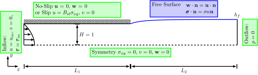
Figure 1: Schematic of the symmetric die swell flow configuration. $L_{1}$ is the length of the die which has fixed boundaries and is of half-height H. $L_{2}$ is the length of the outflow region, the boundaries of which are free to move. Boundary conditions are provided for each surface.

Consider the extrusion of a Newtonian liquid from a planar die. The schematic diagram of the employed planar die geometry is depicted in Figure 1. We consider a die of length $L_{1}$ and height $H$, and an exit region of length $L_{2}$. The length of the die is chosen sufficiently long in order to guarantee a fully developed flow far upstream of the exit plane. In the following, we pay special attention to the following two quantities of interest: the swelling ratio and the pressure exit correction factor. In practice, the extrudate swell ratio is of importance in extrusion processes and the excess pressure loss gives an indication as to how much extra pressure has to be applied to achieve certain swell ratios. The swelling ratio, $\chi_{R}$, is defined as

$$\chi_{R}=\dfrac{h_{f}}{H}$$ (9)

where $H$ is the half-height of the die and $h_{f}$ is the half-height of the liquid jet at the outflow boundary. The swelling ratio is a function of several parameters

$$\chi_{R}(H,\langle u\rangle,\text{Re}\,,B_{sl}),$$ (10)

where $\langle u\rangle$ is the average inflow velocity, Re  is the Reynolds number and $B_{sl}$ is the slip parameter along the die wall.

The dimensionless pressure exit correction factor, $n_{ex}$, is defined as

$$n_{ex}=\dfrac{\Delta p-\Delta p_{0}}{2\sigma_{w}}$$ (11)

where $\Delta p$ is the pressure drop between the inlet and the outlet plane, $\Delta p_{0}$ is the pressure drop between the inlet and the exit of the die for fully developed Poiseuille flow and $\sigma_{w}$ is the shear stress at the channel wall corresponding to fully developed Poiseuille flow. Here, the pressure differences are taken along the centreline. In particular, the pressure drops are given by (Tanner (2002))

$$\Delta p_{0}= p|_{x=-L_{1}}=2\sigma_{w}\frac{L_{1}}{H} \text{Poiseuille flow for }x\in[-L_{1},\,0]$$ (12)

$$\Delta p= p|_{x=-L_{1}}-p|_{x=L_{2}} \text{Extrudate Swell for }x\in[-L_{1},\,L_{2}].$$ (13)

In our computations, we employ the following boundary conditions as depicted in Figure 1 for a half-channel height of $H=1$. We assume the flow is symmetric and along the symmetry line, we set $v=0$ and $\sigma_{xy}=0$. Note that, $\sigma_{xy}=0$ is set through the boundary integral in the momentum equation (25). For the die swell geometry this means that there is no contribution of the Neumann boundary integral in the momentum equation along the symmetry line. At the die wall, we either impose no-slip boundary conditions (i.e. $\mathbf{u}=0$) or Navier’s slip condition. The latter is a mixed boundary condition of Dirichlet and Neumann type. For the extrudate swell geometry depicted in Figure 1, we set $v=0$ and impose $\sigma_{xy}=\frac{1}{B_{sl}}u$ through the Neumann boundary term in the momentum equation (25). This means for the velocity component $u$ along the slip boundary $\Gamma_{sl}$, we obtain the boundary integral

$$\int_{\Gamma_{sl}}\left(\boldsymbol{\sigma}\cdot\mathbf{n}\,\phi_{\mathbf{u}}\right)\mathbf{e}_{x}\,\mathrm{d}\Gamma=\int_{\Gamma_{sl}}\frac{1}{B_{sl}}u\phi_{u}\,\mathrm{d}\Gamma$$ (14)

where $\mathbf{e}_{x}$ is the unit vector in $x$-direction. At the outflow, we employ an open outflow boundary condition. We assume a reference pressure $p=0$ along the outflow boundary and the remaining terms in the Neumann boundary integral along the outflow boundary in the momentum equation are evaluated along with the volume integrals. At inflow, we either impose the parabolic profile

$$u=\dfrac{3}{2}\left(1-y^{2}\right),\quad v=0$$ (15)

in combination with no-slip along the die wall or the profile (Kountouriotis et al. (2013))

$$u=\dfrac{3}{2(1+3B_{sl})}(1-y^{2}+2B_{sl}),\quad\dfrac{\partial u}{\partial y}=\dfrac{-3y}{(1+3B_{sl})},\quad v=0$$ (16)

in combination with the slip boundary condition. In the extrudate swell problem the velocity field undergoes a transition from Poiseuille flow inside the die to plug flow in the free jet. Due to the conservation of energy the flow rate in the die has to be the same as in the uniform plug flow, which yields

$$u_{\mathrm{plug}}=\dfrac{1}{2h_{\mathrm{plug}}}\int_{-H}^{H}u(y)\,\mathrm{d}y$$ (17)

where $h_{\mathrm{plug}}$ is the height of the fluid jet in the uniform flow region and $u(y)$ is the parabolic Poiseuille flow profile. We have $0<u_{\mathrm{plug}}<u_{\mathrm{max}}$, which means that while particles at the free surface accelerate when exiting the die the flow near the centreline decelerates.

For the mesh velocity, we employ the following boundary conditions. We consider the mesh to be fixed at inflow, the die wall and along the symmetry line, i.e. $\mathbf{w}=(w_{x},w_{y})=0$. At the outflow boundary, we allow the mesh to move in the $y$-direction, i.e. $\nabla w_{y}\cdot\mathbf{n}=0$, and fix it in the $x$-direction, $w_{x}=0$. At the free surface, we enforce the kinematic boundary condition through the mesh velocity in terms of a Dirichlet boundary condition for the mesh-velocity, i.e.

$$\mathbf{w}\cdot\mathbf{n}=\mathbf{u}\cdot\mathbf{n}.$$ (18)

To avoid mesh distortion, we choose to move the mesh along the free surface boundary only in the $y$-direction. The mesh is moved with sufficient velocity $w_{y}$ into the $y$-direction to ensure that no particle crosses the interface, that is,

$$w_{x}=0,\quad w_{y}=v+u\frac{n_{x}}{n_{y}}.$$ (19)

3 Numerical Discretisation

3.1 Spectral Element Discretisation

Consider the decomposition of the domain $\Omega_{t}^{\delta}$ into $N_{el}$ non-overlapping elements. These elements are each mapped to a standard element on which the unknowns are approximated using a modal polynomial expansion basis proposed by Dubiner (1991) and extended by Karniadakis and Sherwin (2005) given by

$$\phi_{p}(\xi)=\begin{cases}\dfrac{1-\xi}{2},\quad&p=0,\\[6.45831pt] \left(\dfrac{1-\xi}{2}\right)\left(\dfrac{1+\xi}{2}\right)P_{p-1}^{(1,1)}(\xi),\quad&0<p<P\\[6.45831pt] \dfrac{1+\xi}{2},\quad&p=P.\end{cases}$$ (20)

Here, $\phi_{0}$ and $\phi_{P}$ are the linear finite element basis functions and

$$\phi_{1}(\xi)=\left(\frac{1-\xi}{2}\right)\left(\frac{1+\xi}{2}\right)$$

is the usual quadratic hierarchical expansion mode for quadratic elements. Furthermore, $P$ denotes the highest polynomial order of the hierarchical expansion and $P_{p}^{(\alpha,\beta)}(\xi)$ denotes the $p^{\mathrm{th}}$-order Jacobi polynomial.

Two-dimensional functions $u(\mathbf{x},t)$ can be approximated on two- dimensional standard quadrilaterals, defined as $\Omega_{st}=\{-1\leq\xi_{1},\xi_{2}\leq 1\}$, using a tensor product of the one-dimensional modal expansion basis functions $\phi_{p}$, that is,

$$u(\mathbf{x},t)=\sum_{p=0}^{P}\sum_{q=0}^{P}\hat{u}_{pq}(t)\phi_{p}(\xi_{1})\phi_{q}(\xi_{2})$$ (21)

with the reference coordinates given by

$$\xi_{1}=\left[\chi_{1}^{e,t}\right]^{-1}(x,y),\quad\xi_{2}=\left[\chi_{2}^{e,t}\right]^{-1}(x,y),$$ (22)

involving the inverse of the mapping $\boldsymbol{\chi}^{e}$. Here, the mapping, $\boldsymbol{\chi}^{e}$, between the local coordinates $(\xi_{1},\xi_{2})$ and the physical coordinates $(x,y)$ approximates the geometry with the same order polynomial space as the solution, that is,

$$\mathbf{x}=\boldsymbol{\chi}^{e}(\xi_{1},\xi_{2})=\sum_{p=0}^{P}\sum_{q=0}^{P}\mathbf{\hat{x}}_{pq}\phi_{p}(\xi_{1})\phi_{q}(\xi_{2}).$$ (23)

Details on the construction of this mapping can be found in Karniadakis and Sherwin (2005).

3.2 Weak Formulation

Introducing the function spaces in the current frame with respect to the reference configuration $\hat{\Omega}_{t_{0}}$

$$\mathcal{V}(\Omega_{t})= \left\{\mathbf{u}:\Omega_{t}\times I\rightarrow\mathbb{R}^{d}:\,\,\mathbf{u}=\hat{\mathbf{u}}\circ\mathcal{R}_{t}^{-1},\,\,\hat{\mathbf{u}}\in[H^{1}_{0}(\hat{\Omega}_{t_{0}})]^{d}\right\},$$ (24a)

$$\mathcal{V}_{D}(\Omega_{t})= \left\{\mathbf{u}:\Omega_{t}\times I\rightarrow\mathbb{R}^{d}:\,\,\mathbf{u}=\hat{\mathbf{u}}\circ\mathcal{R}_{t}^{-1},\,\,\hat{\mathbf{u}}\in[H^{1}_{D}(\hat{\Omega}_{t_{0}})]^{d}\right\},$$ (24b)

$$\mathcal{Q}(\Omega_{t})= \left\{q:\Omega_{t}\times I\rightarrow\mathbb{R}^{d}:\,\,q=\hat{q}\circ\mathcal{R}_{t}^{-1},\,\,\hat{q}\in L^{2}(\hat{\Omega}_{t_{0}})\right\},$$ (24c)

$$\mathcal{Q}_{0}(\Omega_{t})= \left\{q:\Omega_{t}\times I\rightarrow\mathbb{R}^{d}:\,\,q=\hat{q}\circ\mathcal{R}_{t}^{-1},\,\,\hat{q}\in L^{2}_{0}(\hat{\Omega}_{t_{0}})\right\},$$ (24d)

the weak formulation of the system of equations  (6) leads to the following problem definition.

Problem 3.1 (Weak formulation of incompressible Navier-Stokes equations).

For almost every $t\in I$ find $t\rightarrow\left(\mathbf{u}(t),p(t)\right)\in\mathcal{V}_{D}(\Omega_{t})\times\mathcal{Q}_{0}(\Omega_{t})$ such that, for all $\left(\phi_{\mathbf{u}},\psi\right)\in\mathcal{V}(\Omega_{t})\times\mathcal{Q}(\Omega_{t})$

$$\text{Re}\,\left(\left.\dfrac{\partial\mathbf{u}}{\partial t}\right|_{\mathbf{Y}}+\left(\mathbf{u}-\mathbf{w}\right)\cdot\nabla_{\boldsymbol{x}}\mathbf{u},\,\phi_{\mathbf{u}}\right)_{\Omega_{t}}+\left(2\mathbf{D}_{\boldsymbol{x}},\,\nabla_{\boldsymbol{x}}\phi_{\mathbf{u}}\right)_{\Omega_{t}}$$

$$-\left(p,\,\nabla_{\boldsymbol{x}}\cdot\phi_{\mathbf{u}}\right)_{\Omega_{t}}-\left\langle\boldsymbol{\sigma}\cdot\mathbf{n},\,\phi_{\mathbf{u}}\right\rangle_{\Gamma_{N}(t)}-\left\langle\sigma\kappa\cdot\mathbf{n},\,\phi_{\mathbf{u}}\right\rangle_{\Gamma_{f}(t)} =0,$$ (25)

$$\left(\nabla_{\boldsymbol{x}}\cdot\mathbf{u},\,\psi\right)_{\Omega_{t}} =0,$$ (26)

where $\Gamma_{N}(t)$ is the Neumann boundary and $\Gamma_{f}(t)$ is the free surface boundary.

We choose the same trial and test function space for the mesh velocity as for the fluid velocity, i.e. we choose

$$\mathcal{W}(\Omega_{t})\equiv\mathcal{V}(\Omega_{t})$$ (27)

and we solve Equation (8) with the boundary conditions (7) using a continuous Galerkin method. The weak formulation for the mesh movement can therefore be expressed as below.

Problem 3.2 (Weak Formulation Mesh Velocity).

For almost every $t\in I$ find $t\rightarrow\mathbf{w}(t)\in\mathcal{V}_{D}(\Omega_{t})$ such that, for all $\phi_{\mathbf{w}}\in\mathcal{V}(\Omega_{t})$

$$\left(\nabla\mathbf{w},\nabla\phi_{\mathbf{w}}\right)_{\Omega_{t}}=0$$ (28)

subject to the boundary conditions (7).

The position of the new nodes of the mesh can be obtained via Equation (4), that is,

$$\left.\dfrac{\partial\boldsymbol{x}(\mathbf{Y},t)}{\partial t}\right|_{\mathbf{Y}}=\left.\dfrac{\partial\mathcal{R}_{t}(\mathbf{Y})}{\partial t}\right|_{\mathbf{Y}}=\mathbf{w}(\boldsymbol{x},t).$$ (29)

3.3 Discrete ALE formulation

As mentioned above, we have two referential domains to consider in the ALE formulation. Firstly, let $\Omega_{t}^{\delta}$ be the union of all non-overlapping mesh elements in the Eulerian frame at time $t$ and secondly, let $\hat{\Omega}_{t_{0}}^{\delta}$ denote the union of all mesh elements in the referential frame. Consider the following discrete trial and test function spaces

$$\mathcal{V}_{D}^{\delta}(\Omega_{t}^{\delta})=\left\{\mathbf{u}:\Omega_{t}^{\delta}\times I\rightarrow\mathbb{R}^{d}:\,\,\mathbf{u}=\hat{\mathbf{u}}\circ[\mathcal{R}_{t}^{\delta}]^{-1},\,\,\hat{\mathbf{u}}\in[H^{1}_{D}(\Omega_{t_{0}}^{\delta})]^{d}\cap[\mathcal{P}_{P}^{c}(\Omega_{t_{0}}^{\delta})]^{d}\right\}$$ (30)

for the fluid and mesh velocities and

$$\mathcal{Q}^{\delta}(\Omega_{t}^{\delta})=\left\{q:\Omega_{t}^{\delta}\times I\rightarrow\mathbb{R}:\,\,q=\hat{q}\circ[\mathcal{R}_{t}^{\delta}]^{-1},\,\,\hat{q}\in L^{2}(\Omega_{t_{0}}^{\delta})\cap[\mathcal{P}_{P-2}(\Omega_{t_{0}}^{\delta})]^{d})\right\},$$ (31)

for the pressure field. Alternatively, these spaces can be expressed as (see Pena (2009))

$$\mathcal{V}_{D}^{\delta}(\Omega_{t}^{\delta}) =[H^{1}_{D}(\Omega_{t}^{\delta})]^{d}\cap[\mathcal{P}_{P}^{c}(\Omega_{t}^{\delta})]^{d},$$ (32)

$$\mathcal{Q}^{\delta}(\Omega_{t}^{\delta}) =L^{2}(\Omega_{t}^{\delta})\cap[\mathcal{P}_{P-2}(\Omega_{t}^{\delta})]^{d}.$$ (33)

Here, $\mathcal{P}_{P}^{c}(\Omega_{t_{0}}^{\delta})$ denotes the globally continuous space of polynomials of degree $P$ over the reference mesh, that is,

$$\mathcal{P}_{P}^{c}(\Omega_{t_{0}}^{\delta})=\left\{\left.g^{\delta}:\Omega_{t_{0}}^{\delta}\rightarrow\mathbb{R}\right|\,\,g^{\delta}\in\mathcal{C}^{0}(\overline{\Omega_{t_{0}}}),\,\,\left.g^{\delta}\right|_{\Omega_{t_{0}}^{e}}\circ[\boldsymbol{\chi}^{e}(t_{0})]^{-1}\in\mathcal{P}_{P}(\Omega_{st})\right\}.$$ (34)

$\mathcal{P}_{P}(\Omega_{t_{0}}^{\delta})$ denotes the space of piecewise continuous polynomials of degree $P$ over the reference mesh, that is,

$$\mathcal{P}_{P}(\Omega_{t_{0}}^{\delta})=\left\{\left.g^{\delta}:\Omega_{t_{0}}^{\delta}\rightarrow\mathbb{R}\right|\,\,g^{\delta}\in L^{2}(\overline{\Omega_{t_{0}}}),\,\,\left.g^{\delta}\right|_{\Omega_{t_{0}}^{e}}\circ[\boldsymbol{\chi}^{e}(t_{0})]^{-1}\in\mathcal{P}_{P}(\Omega_{st})\right\}.$$ (35)

$\mathcal{P}_{P}^{c}(\Omega_{t}^{\delta})$ denotes the globally continuous polynomial space over the Eulerian mesh and $\mathcal{P}_{P}(\Omega_{t}^{\delta})$ denotes the piecewise continuous polynomial space over the Eulerian mesh. Here, $\left.g^{\delta}\right|_{\Omega_{t_{0}}^{e}}$ denotes the restriction of $g^{\delta}$ to the spectral element $\Omega_{t_{0}}^{e}$, $\mathcal{P}_{P}(\Omega_{st})$ is the space of polynomials of degree $P$ defined on the standard element given by the expansion basis (20). Note that, the pressure is discretised with polynomials of order 2 lower than the velocities to satisfy the LBB condition (Brezzi, 1974). The spaces $\mathcal{V}_{D}^{\delta}(\Omega_{t}^{\delta})$ and $\mathcal{Q}^{\delta}(\Omega_{t}^{\delta})$ include the discrete ALE mapping, which can be expressed as (Nobile, 2001)

$$\left.\mathcal{R}_{t}^{\delta}\right|_{\Omega_{t_{0}}^{e}}=\boldsymbol{\chi}^{e}(t)\circ[\boldsymbol{\chi}^{e}(t_{0})]^{-1}\quad\forall\Omega_{t_{0}}^{e},$$ (36)

involving the geometrical mappings, $\boldsymbol{\chi}^{e}(t)$, at each $t$, from the standard element $\Omega_{st}$ to each element $\Omega_{t}^{e}$, that is,

$$\mathbf{x}(\xi_{1},\xi_{2})=\boldsymbol{\chi}^{e}(t;\xi_{1},\xi_{2})=\sum_{p=0}^{P}\sum_{q=0}^{P}\mathbf{\hat{x}}_{pq}(t)\phi_{p}(\xi_{1})\phi_{q}(\xi_{2}),$$ (37)

where $\mathbf{\hat{x}}_{pq}(t)$ denotes the expansion coefficients at time $t$ and the iso-parametric mapping, $\boldsymbol{\chi}^{e}(t_{0})$, from $\Omega_{st}$ to $\Omega_{t_{0}}^{e}$, defined as

$$\mathbf{Y}(\xi_{1},\xi_{2})=\boldsymbol{\chi}^{e}(t_{0};\xi_{1},\xi_{2})=\sum_{p=0}^{P}\sum_{q=0}^{P}\mathbf{\hat{Y}}_{pq}\phi_{p}(\xi_{1})\phi_{q}(\xi_{2}).$$ (38)

Using these space definitions and an implicit Euler time-integration scheme, the semi-discrete Navier-Stokes equations are expressed as follows.

Problem 3.3 (Semi-discrete Navier-Stokes ALE formulation).

For each $n$, let $t_{n}=t_{0}+n\Delta t$, find $(\mathbf{u}^{n+1}_{\delta},p^{n+1}_{\delta})\in(\mathcal{V}^{\delta}_{D}(\Omega_{t_{n+1}}^{\delta})\times\mathcal{Q}_{0}^{\delta}(\Omega_{t_{n+1}}^{\delta}))$ with $\mathbf{u}_{\delta}^{0}=\mathbf{u}_{0,\delta}$ in $\Omega_{t_{0}}^{\delta}$ such that

$$\begin{split}&\text{Re}\,\left(\dfrac{\mathbf{u}^{n+1}_{\delta}-\mathbf{u}^{n}_{\delta}}{\Delta t},\,\phi_{\mathbf{u}}\right)_{\Omega_{t_{n+1}}^{\delta}}+\left([\left(\mathbf{u}^{*}_{\delta}-\mathbf{w}^{n+1}_{\delta}\right)\cdot\nabla_{\boldsymbol{x}}]\mathbf{u}^{n+1}_{\delta},\,\phi_{\mathbf{u}}\right)_{\Omega_{t_{n+1}}^{\delta}}\\ &+\left(2\mathbf{D}^{n+1}_{\boldsymbol{x},\delta},\,\nabla_{\boldsymbol{x}}\phi_{\mathbf{u}}\right)_{\Omega_{t_{n+1}}^{\delta}}-\left(p^{n+1}_{\delta},\,\nabla_{\boldsymbol{x}}\cdot\phi_{\mathbf{u}}\right)_{\Omega_{t_{n+1}}^{\delta}}\\ &-\left\langle\boldsymbol{\sigma}^{n+1}_{\delta}\cdot\mathbf{n},\,\phi_{\mathbf{u}}\right\rangle_{\Gamma_{N}(t_{n+1})}-\left\langle\sigma\kappa_{S}\cdot\mathbf{n}_{S},\,\phi_{\mathbf{u}}\right\rangle_{\Gamma_{f}(t_{n+1})}=0,\end{split}$$ (39)

$$\left(\nabla_{\boldsymbol{x}}\cdot\mathbf{u}^{n+1}_{\delta},\,\psi\right)_{\Omega_{t_{n+1}}^{\delta}}=0,$$ (40)

for all $\left(\phi_{\mathbf{u}},\psi\right)\in(\mathcal{V}^{\delta}(\Omega_{t_{n+1}}^{\delta})\times\mathcal{Q}^{\delta}(\Omega_{t_{n+1}}^{\delta}))$. Here, we linearise the convective term in the momentum equation by setting $\mathbf{u}^{*}_{\delta}=\mathbf{u}^{n}_{\delta}$, which is an extrapolation of the velocity of the same order as the implicit Euler scheme. Note that, the index $S$ for normals and curvature in the boundary integral over $\Gamma_{f}(t_{n+1})$ indicates that these quantities are determined from a cubic spline representation of the free surface according to equation (50) and (51) defined below.

3.4 Matrix formulation

The discrete ALE formulation involves the following matrices

$$\mathbf{M}^{e}(t)[j][i] = \dfrac{\text{Re}\,}{\Delta t}\left(\phi_{u}^{i},\phi_{u}^{j},\right)_{{\Omega_{t}}^{e,\delta}}^{\delta},$$ (41)

$$\mathbf{K}^{e}(t)[j][i] = \left(\nabla_{\boldsymbol{x}}\phi^{i}_{\mathbf{u}}+[\nabla_{\boldsymbol{x}}\phi^{i}_{\mathbf{u}}]^{T},\,\nabla_{\boldsymbol{x}}\phi^{j}_{\mathbf{u}}\right)_{{\Omega_{t}}^{e,\delta}}^{\delta},$$ (42)

$$-\left\langle\left(\nabla_{\boldsymbol{x}}\phi^{i}_{\mathbf{u}}+[\nabla_{\boldsymbol{x}}\phi^{i}_{\mathbf{u}}]^{T}\right)\cdot\mathbf{n},\,\phi^{j}_{\mathbf{u}}\right\rangle_{\Gamma_{N}(t)},$$

$$\mathbf{B}^{e}(t;\mathbf{u}_{\delta},\mathbf{w}_{\delta})[j][i] = \left([\left(\mathbf{u}_{\delta}-\mathbf{w}_{\delta}\right)\cdot\nabla_{\boldsymbol{x}}]\phi_{\mathbf{u}}^{i},\,\phi^{j}_{\mathbf{u}}\right)_{{\Omega_{t}}^{e,\delta}}^{\delta},$$ (43)

$$\mathbf{D}^{e}(t)[j][i] = \left(\nabla_{\boldsymbol{x}}\phi_{u}^{i},\psi^{j}\right)_{{\Omega_{t}}^{e,\delta}}^{\delta},$$ (44)

$$\mathbf{b}(t)[j] = \left\langle\sigma\kappa_{S}\cdot\mathbf{n}_{S},\,\phi^{j}_{\mathbf{u}}\right\rangle_{\Gamma_{f}(t)},$$ (45)

and a modified Helmholtz matrix

$$\mathbf{H}^{e}(t)[j][i]:=\mathbf{M}^{e}(t)[j][i]+\mathbf{K}^{e}(t)[j][i]+\mathbf{B}^{e}(t;\mathbf{u}_{\delta},\mathbf{w}_{\delta})[j][i].$$ (46)

The equation system (39)-(40) can then be written for each element in algebraic form as

$$\mathbf{H}_{g}(t_{n+1})\hat{\mathbf{u}}^{n+1}_{g}-\mathbf{D}_{g}(t_{n+1})^{T}\hat{\mathbf{p}}^{n+1}_{g} =\mathbf{M}(t_{n+1})\hat{\mathbf{u}}^{n}+\mathbf{b}(t_{n+1}),$$

$$\mathbf{D}_{g}(t_{n+1})\textit{}\hat{\mathbf{u}}_{g}^{n+1} =0,$$ (47)

where $\hat{\mathbf{u}}_{g}$ and $\hat{\mathbf{p}}_{g}$ are the vectors of unknown global coefficients, $\mathbf{H}_{g}$, $\mathbf{D}_{g}=(\mathbf{D}_{x_{1}},\mathbf{D}_{x_{2}})$ are the global matrices assembled from the elemental matrix contributions. The resulting system of equations is then solved using a multi-level static condensation technique introduced by Ainsworth and Sherwin (1999), Sherwin and Ainsworth (2000) and Karniadakis and Sherwin (2005) for the Stokes equations in fixed domains.

3.5 Discretisation of Mesh Movement

Even though solving Problem 3.2 yields continuous mesh movement, the free surface boundary might not be sufficiently smooth. The free surface boundary undergoes the largest deformation and its movement involves the evaluation of outward normals, $\mathbf{n}$, in Equation (7), across multiple elements. Note that, a standard Galerkin method with a $C^{0}$-continuity across elements is not sufficient to determine a well-defined normal at element edges. To alleviate this problem, we represent the free surface using a cubic spline, $S(x,t)\in\mathcal{C}^{2}(\Gamma_{f})$ to ensure sufficient smoothness of free surface boundary edges of the mesh. The cubic spline can then be used to determine the unit outward normals $\mathbf{n}$ and the curvature $\kappa$ of the free surface using

$$\mathbf{n}_{S}(t)=\dfrac{1}{\sqrt{S^{\prime}(x,t)^{2}+1}}\left(\begin{array}[]{c}-S^{\prime}(x,t)\\ 1\end{array}\right),$$ (50)

$$\kappa_{S}(t)=\dfrac{|S^{\prime\prime}(x,t)|}{(1+S^{\prime}(x,t)^{2})^{3/2}}.$$ (51)

These expressions are then used to evaluate the free surface boundary condition for the mesh velocity given by Equation (7) and the free surface boundary integral in the momentum equation

$$\int\limits_{\Gamma_{f}}\sigma\kappa_{S}\mathbf{n}_{S}\,\phi_{\mathbf{u}}\,\mathrm{d}\Gamma.$$ (52)

For given $\mathbf{u}^{n}$, we perform the mesh movement in the following way. First, we determine the cubic spline through all the quadrature points along the free surface. Let $(x_{i},y_{i})$, $1\leq i\leq N,$ be the physical coordinates of the $N$ quadrature points along the free surface. Then, we construct a cubic spline $S(x,t)=S_{i}(x,t)$ for each $x_{i}\leq x\leq x_{i+1}$ through

$$S_{i}(x,t)=a_{i}(x-x_{i})^{3}+b_{i}(x-x_{i})^{2}+c_{i}(x-x_{i})+d_{i}$$ (53)

where we enforce continuity

$$S_{i-1}(x_{i},t)=S_{i}(x_{i},t),$$

$$S_{i}(x_{i+1},t)=S_{i+1}(x_{i+1},t)$$ (54)

and smoothness

$$S_{i-1}^{\prime}(x_{i},t)=S_{i}^{\prime}(x_{i},t),$$

$$S_{i-1}^{\prime\prime}(x_{i},t)=S_{i}^{\prime\prime}(x_{i},t),$$

$$S_{i}^{\prime}(x_{i+1},t)=S_{i+1}^{\prime}(x_{i+1},t),$$

$$S_{i}^{\prime\prime}(x_{i+1},t)=S_{i+1}^{\prime\prime}(x_{i+1},t).$$ (55)

We employ the not-a-knot boundary condition on the spline, that is,

$$S^{\prime\prime\prime}_{1}(x_{2})=S^{\prime\prime\prime}_{2}(x_{2}),$$ (56)

$$S^{\prime\prime\prime}_{N-1}(x_{N-1})=S^{\prime\prime\prime}_{N-2}(x_{N-1}).$$ (57)

We then solve the elliptic problem (28) using the continuous Galerkin method, determining

$$\mathbf{L}_{g}\hat{\tilde{\mathbf{w}}}_{g}=0,$$ (58)

where $\mathbf{L}_{g}$ is the global Laplace matrix given by

$$\mathbf{L}^{e}(t)[j][i]=\left(\nabla_{\boldsymbol{x}}\phi^{i}_{\mathbf{w}},\,\nabla_{\boldsymbol{x}}\phi^{j}_{\mathbf{w}}\right)_{{\Omega_{t}}^{e,\delta}}^{\delta},$$ (59)

subject to the boundary conditions (7), which include the normal determined by the cubic spline according to (50).

The mesh velocity resulting from the solution of Equation (58), denoted by $\tilde{\mathbf{w}}$, is then used to update the coordinates of the mesh nodes using a third order Adams-Bashforth-Scheme for Equation (4), that is,

$$\mathbf{X}^{n+1}=\mathbf{X}^{n}+\frac{\Delta t}{12}(23\tilde{\mathbf{w}}-16\mathbf{w}^{n}+5\mathbf{w}^{n-1}).$$ (60)

This equation is solved pointwise in the strong form for each quadrature point. However, in practice, we do not move all the mesh nodes of every element. We only move all the quadrature points along the free surface boundary introducing curved edges along the free surface boundary. In the interior of the domain, we just move the corner vertices of every element keeping the interior edges of the domain straight.

Using the new coordinates of all mesh nodes, we compute the mesh velocity at the new time level pointwise as

$$\mathbf{w}^{n+1}=\dfrac{\mathbf{X}^{n+1}-\mathbf{X}^{n}}{\Delta t}.$$ (61)

3.6 Algorithm Summary

In Summary, the solution procedure is outlined in Algorithm 3.6

[shadowbox]ALE scheme.u^n,p^n t = t_0

t≤t_fin MoveMeshu^n,p^n,τ^n Construct Cubic Spline through Free Surface Boundary.

Set BC for Mesh Velocity (see (7)).

Solve Elliptic Problem for Mesh Velocity (LABEL:equ:_mesh_veldiscrete).

w^n+1

Compute New Mesh Coordinates $\mathbf{X}^{n+1}$.

Construct New Parametric Mappings $\boldsymbol{\chi}^{e}(t_{n+1})$.

Ω_t_n+1 Set Boundary Conditions for $\mathbf{u}$ and $p$.

SolveCoupledSystemu^n,p^n,w^n+1 Solve Coupled System of Velocity, Pressure

u^n+1,p^n+1 t_n+1 t_n + Δt

n+1 n

4 Numerical Results

4.1 Mesh Configuration

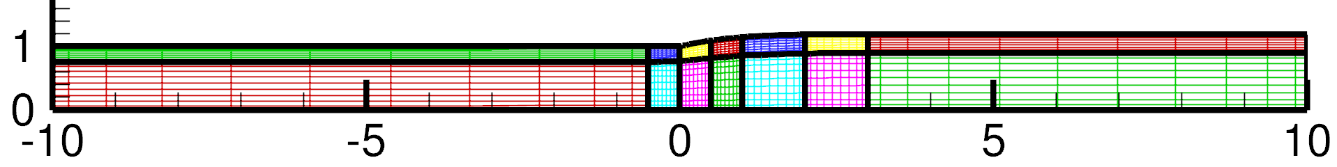
(a)

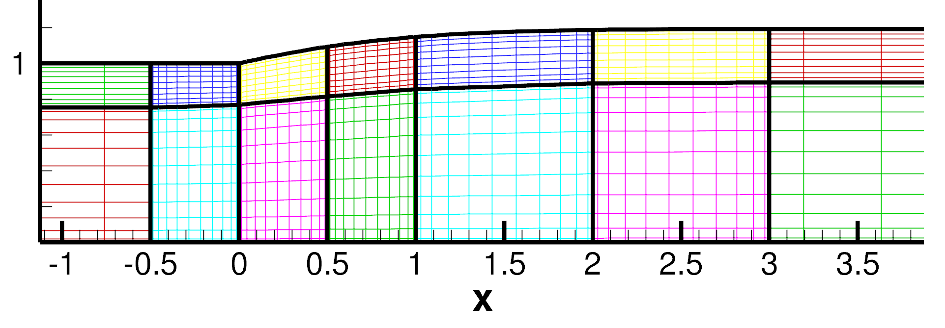
(b)

Figure 2: Mesh configuration used for the extrudate swell computation.

We use a mesh consisting of $N_{el}=14$ elements as shown in Figure 2 and refine the mesh by increasing the polynomial order $P$. We consider a die of length $L_{1}=10$ and an exit region of length $L_{2}=10$. The entry length is sufficient to guarantee a fully developed flow far upstream from the exit of the die. The exit length is chosen sufficiently long to allow the free surface to reach a constant downstream height for a large range of Reynolds numbers. For high Reynolds numbers, the free jet length might be insufficient to guarantee a fully developed plug flow profile at outflow. However, the use of the open outflow boundary condition enables us to predict the correct swelling ratios truncated at the outflow boundary location (see Mitsoulis et al. (2012)). Throughout this section, we choose a time step of $5\times 10^{-3}$.

4.2 Numerical results for $Re=0$

Table 1: Newtonian swelling ratios for $\text{Re}\,=0$

	Method	DOF	$\chi_{R}$
Crochet and Keunings (1982)	FEM	562	1.200
		1178	1.196
Reddy and Tanner (1978)	FEM	254	1.199
Mitsoulis et al. (2012)	FEM	11270	1.191
		30866	1.186
Georgiou and Boudouvis (1999)	FEM (SFEM)	7528	1.1919 (1.1863)
	FEM (SFEM)	12642	1.1888 (1.1863)

Inertialess Newtonian extrudate swell has been investigated in a number of publications. Table 1 summarises some of the swelling ratios obtained by a range of authors for plane Newtonian die swell. Tanner (2002) used the results in the literature to estimate an extrapolated value for planar die swell of $\chi_{R}=1.190\pm 0.002$. In general, an increase in the number of degrees of freedom yields less swelling.

Table 2: Comparison of swell ratios and exit pressure corrections for increasing number of degrees for freedom (DOF) between our algorithm and Taliadorou et al. (2007).

Spectral/hp method				Taliadorou et al. (2007) FEM
P	DOF	$h_{f}$	$n_{ex}$	DOF	$h_{f}$	$n_{ex}$
8	2624	1.1928	0.1507
10	4116	1.1912	0.1503	37208	1.1953	0.1514
12	5944	1.1901	0.1497	43320	1.1908	0.1491
14	8108	1.1900	0.1491	49864	1.1893	0.1482
16	10608	1.1891	0.1485	60490	1.1878	0.1473

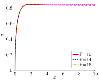
(a) Velocity component $u$ along the free surface.

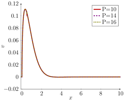
(b) Velocity component $v$ along the free surface.

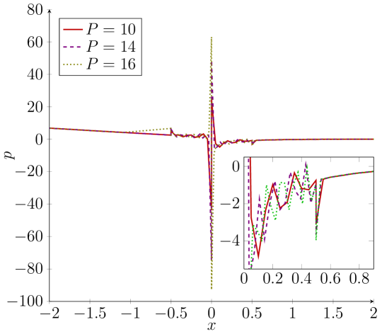
(c) Pressure $p$ along the die wall and the free surface.

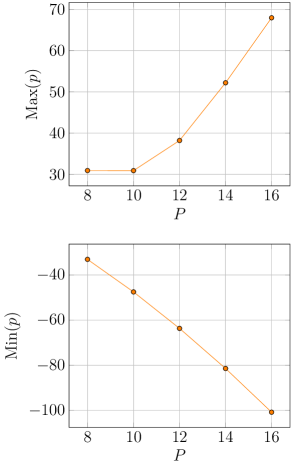
(d) Pressure minima and maxima.

Figure 3: Influence of $P$-mesh refinement on LABEL:sub@subfig:_swell_newton_refinement_u the velocity components $u$, LABEL:sub@subfig:_swell_newton_refinement_v $v$ and LABEL:sub@subfig:_swell_newton_refinement_p pressure $p$ along the free surface and the increase of maximum and minimum values of the pressure at the singularity with increasing polynomial order LABEL:sub@subfig:_p_minmax_refinement.

Table 2 lists a comparison of the pressure exit correction for $\text{Re}\,=0$ of our scheme and the swell ratio for increasing mesh refinement with the results obtained by Taliadorou et al. (2007). We obtain close agreement for a much smaller number of degrees of freedom, which demonstrates that $p$-refinement is effective for the Newtonian extrudate swell even though the result is polluted by Gibbs oscillations in the pressure around the singularity (Figure 3c). The Gibbs oscillations in the pressure stay confined to the elements adjacent to the singularity. Increasing the Reynolds number leads to a dampening in the oscillations in the elements adjacent to the singularity and the extreme values of the pressure at the singularity decrease significantly (Figure 11b). As shown in Figure 3c increasing the polynomial order yields an increase in the number of oscillations. However, the amplitude of each oscillation is reduced with increasing polynomial order $P$. Increasing the polynomial order also has the effect of exponentially increasing the maximum value of the pressure and sharply increasing the minimum value of the pressure at the singularity which reflects an improved approximation of the infinite pressure value at the singularity (Figure 3d). While the infinite pressure values at the singularity hamper the rate of convergence of the numerical pressure solution, the values of the velocity components along the free surface are converged for $P\geq 10$ (see Figure 3LABEL:sub@subfig:_swell_newton_refinement_u, LABEL:sub@subfig:_swell_newton_refinement_v).

4.3 Impact of inertia

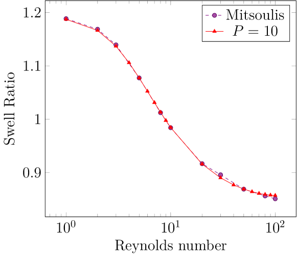
Figure 4: Comparison of swell ratios for Newtonian fluid from the current study ($P=10$) with Mitsoulis et alMitsoulis et al. (2012).

Table 3: Comparison of Newtonian die swell ratio for increasing Reynolds number with Mitsoulis et al. (2012).

Re	Mitsoulis et al. (2012)	$P=10$	Re	Mitsoulis et al. (2012)	$P=10$
0	1.1915	1.1912	10	0.9842	0.9846
1	1.1885	1.1873	20	0.9168	0.9161
2	1.1687	1.1665	30	0.8960	0.8903
3	1.1394	1.1370	40		0.877
4		1.1060	50	0.8691	0.8692
5	1.0775	1.0774	60		0.8643
6		1.0525	70		0.8611
7		1.0313	80	0.8564	0.8592
8	1.0124	1.0132	90		0.8579
9		0.9977	100	0.85103	0.8573

Inertia causes a decrease of the swelling and the liquid jet eventually contracts for sufficiently high Reynolds numbers. We performed computations for Reynolds numbers ranging from 0 to 100. We start by computing the extrudate swell for $\text{Re}\,=0$ and initialise this computation with the solution of the corresponding stick-slip problem. After having obtained the extrudate swell for $\text{Re}\,=0$, we increase the Reynolds number in steps of 1 from 1 to 10 and in steps of 10 from 10 to 100, each time using the result of the converged extrudate swell of the previous lower Reynolds number as the initial condition. As the convergence criterion, we choose a change of the maximum absolute value of all variables including the mesh velocity of less than $10^{-6}$. Figure 4 and Table 3 shows the comparison of the swelling ratios obtained with our algorithm with the results of Mitsoulis et al. (2012), which are in excellent agreement.

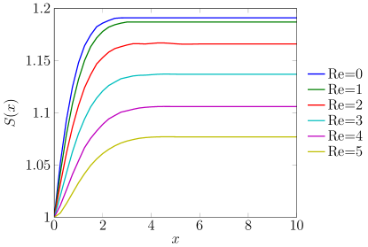
(a)

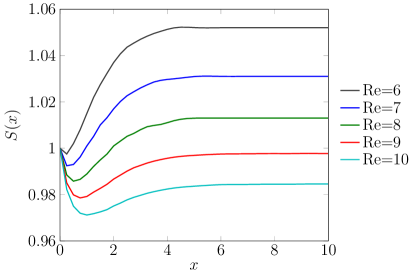
(b)

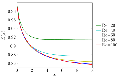
(c)

Figure 5: Free surface spline profiles for Newtonian extrudate swell for $P=10$ for a range of Reynolds numbers.

Figure 5 displays the corresponding free surface spline profiles. We observe that the swelling ratio decreases at an accelerating pace with increasing Reynolds number until $\text{Re}\,=6$. For $\text{Re}\,=6$, we see the onset of a delayed die swell in which the fluid surface first goes through a minimum before it swells again. The delay in the swelling of the jet increases with increasing Reynolds number from $\text{Re}\,=6$ to $\text{Re}\,=10$. For $\text{Re}\,=9$ and $\text{Re}\,=10$, the fluid contracts ($\chi_{R}<1$) but still experiences some swelling after going through a minimum near the die exit. For $\text{Re}\,=20$ to $\text{Re}\,=100$ the fluid does not experience any delayed swelling and contracts. For $10<\text{Re}\,<40$ the fluid contracts very fast with increasing Reynolds number. This trend in the contraction rate with increasing Reynolds number then slows down and approaches a limit for $40<\text{Re}\,<100$. The limit for infinite Reynolds number was estimated by Tillett (1968) who performed a boundary layer analysis for a free Newtonian jet and predicted a limiting value of $\chi_{R}=0.8333$ for infinite Reynolds number.

(a)
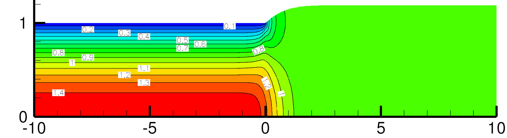
(b)
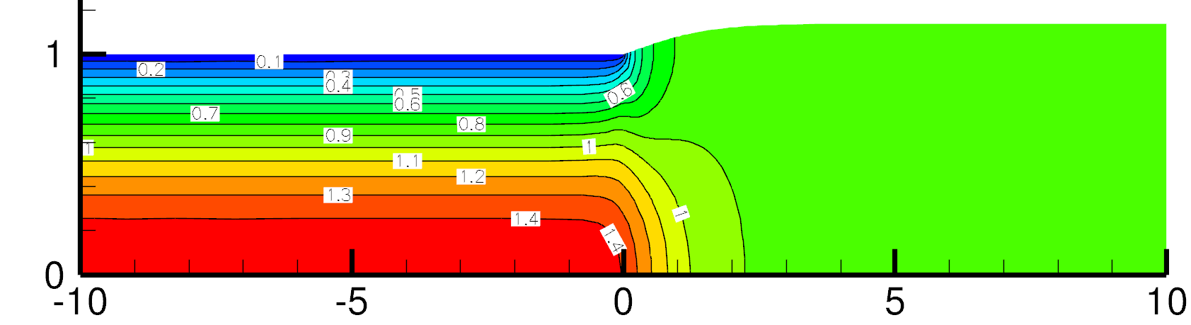
(c)
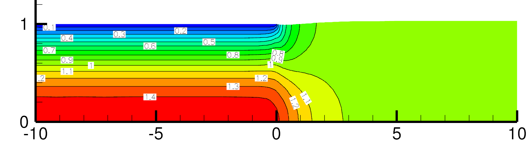
(d)
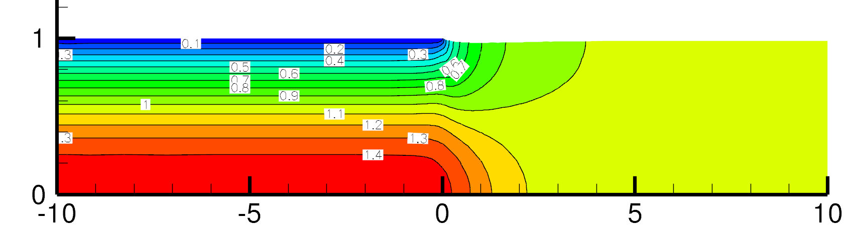
(e)

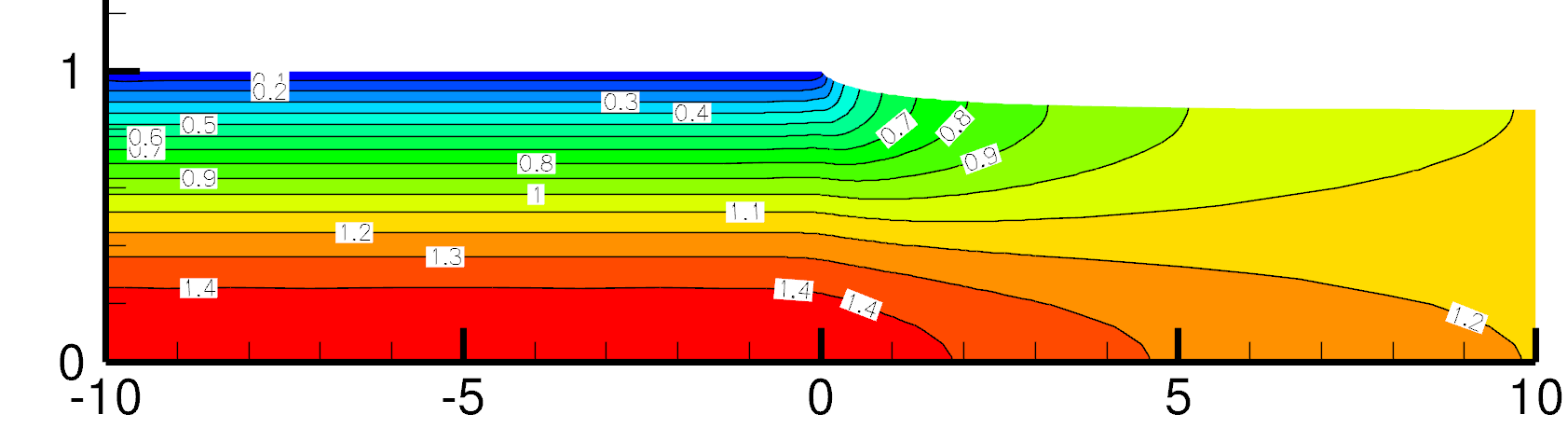
Figure 6: Horizontal velocity component $u$ for $P=10$ for (a) $Re=0$, (b) $Re=3$, (c) $Re=7$, (d) $Re=10$ and (e) $Re=50$. Contours are indicated at intervals of $0.1$.

We explore the contour plots of the velocity field for a range of Reynolds numbers in Figures 6 (horizontal velocity component $u$),  8 (vertical velocity component $v$). With increasing Reynolds number the horizontal velocity increases along the centreline, the vertical velocity near the singularity induced by the sudden change in the boundary condition decreases and the transition zone under the free surface from Poiseuille flow in the die to plug flow is extended downstream. This shows that with increasing Reynolds number the particles along the centreline are accelerated and decelerated near the free surface yielding the contraction of the free fluid jet. This is indeed the behaviour we would expect as particles leaving the die will deviate less from their initial path for increasing inertia. As pointed out by Mitsoulis et al. (2012) in order to accommodate the whole transition zone the domain length of the free fluid jet should be chosen as $L_{2}=\text{Re}\,$. However, we employ open boundary conditions at outflow which enable us to compute the extrudate swell accurately in the truncated domain with $L_{2}=10$. As demonstrated by Mitsoulis and Malamataris (2011) the results for extrudate swell with a domain length $L_{2}=6$ are virtually identical with those from long domains with $L_{2}=\text{Re}\,$, for all variables, when using the open boundary condition at outflow. However, in this case, the swell ratio results are only correct up to the truncated length as they continuously drop beyond the truncated domain. A small discrepancy between swell ratios for different domain lengths can therefore be expected.

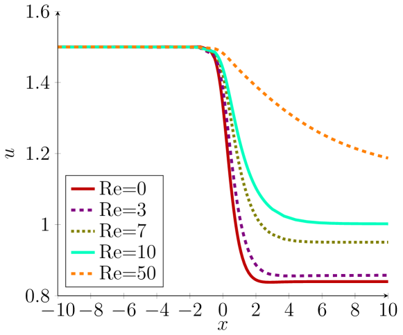
(a) Velocity component $u$ along symmetry line ($v=0$).

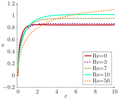
(b) Velocity component $u$ along free surface.

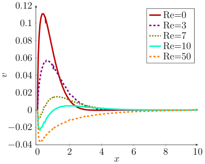
(c) Velocity component $v$ along free surface.

Figure 7: Dependency of velocity components along LABEL:sub@subref:_centreline_newt_swell_u the symmetry line and LABEL:sub@subref:_free_surface_newt_swell_u- LABEL:sub@subref:_free_surface_newt_swell_v along the free surface on the Reynolds number.

(a)
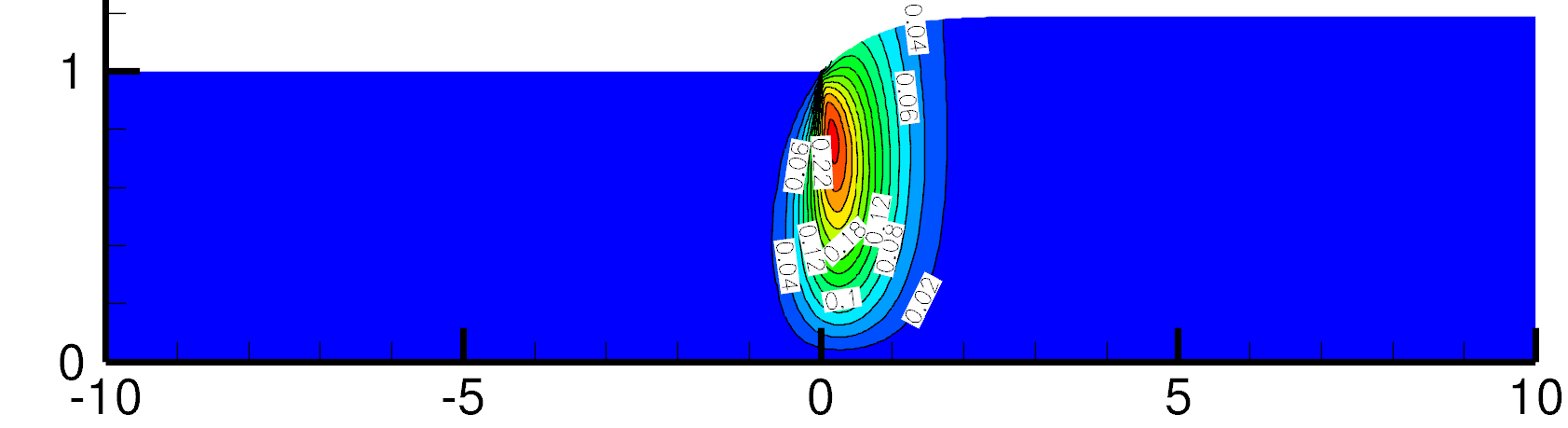
(b)
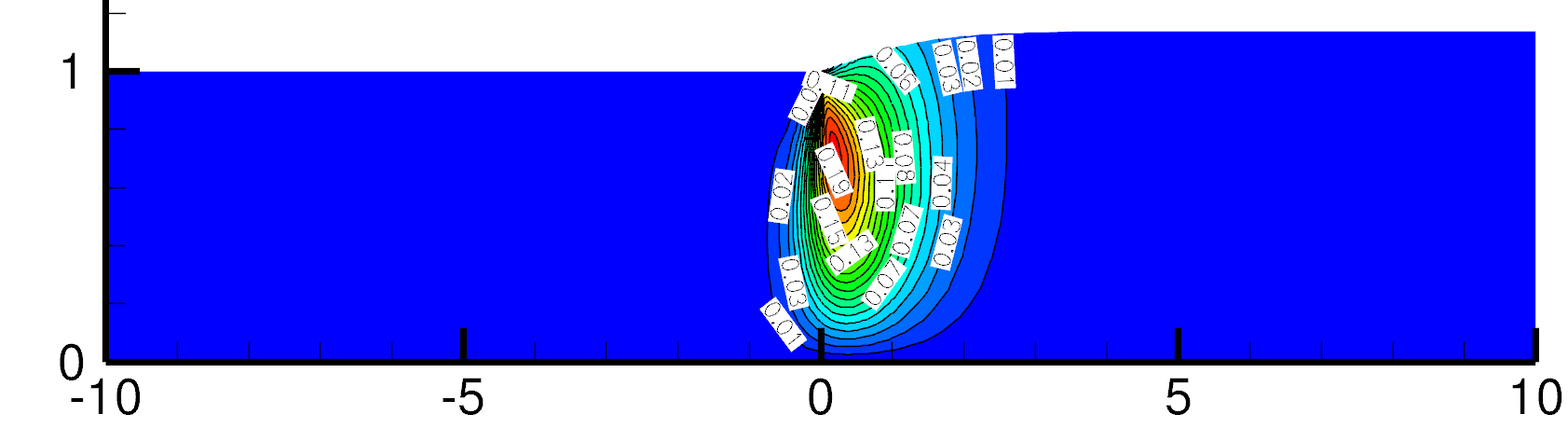
(c)
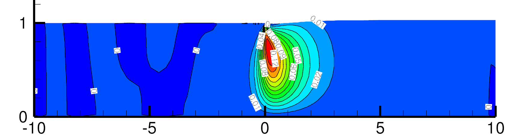
(d)
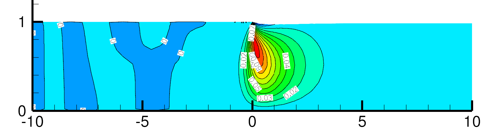
(e)

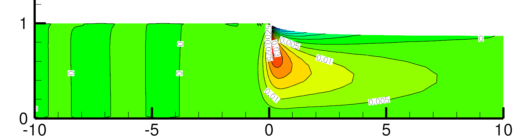
Figure 8: Vertical velocity $v$ for $P=10$ for (a) $Re=0$, (b) $Re=3$, (c) $Re=7$, (d) $Re=10$ and (e) $Re=50$.

To investigate the transition from Poiseuille flow to plug flow for increasing Reynolds number further, we plot the velocity and pressure along different paths in the domain. Figure 7 displays the velocity components along the symmetry line (i.e. $v=0$) and along the free surface boundary. In Figure 7a, we see the smooth transition of the velocity field from the maximum of the parabolic profile to the average plug flow velocity given by Equation (17), i.e. $u_{plug}=1/\chi_{R}$. As the swell decreases with increasing Reynolds number the plug flow value of the velocity increases with increasing Reynolds number. With increasing Reynolds number the change from the maximum parabolic value of the velocity component $u$ to the plug flow value shifts further downstream. For $\text{Re}\,=0$, the velocity reaches the plug flow value at around $x\approx 3$, for $\text{Re}\,=10$ at $x\approx 6$ and for $\text{Re}\,=50$ the plug flow value is not reached within our computational domain. However, as pointed out above, due to the use of open boundary conditions at outflow, the velocity and pressure profiles stay accurate even if they are truncated at outflow.

Along the free surface boundary (Figure 7b), the velocity component $u$ increases sharply near the die exit until it reaches the plug flow value while the velocity component $v$ goes through a maximum near the die exit for $\text{Re}\,=0$ and $\text{Re}\,=3$ and through a minimum for $\text{Re}\,>7$, when particles are no longer constrained by the no-slip boundary condition (Figure 7c). This causes the swell (for $v>0$) or the contraction (for $v<0$) of the free surface near the die exit until the surface is sufficiently curved to obtain a zero total shear stress (i.e. $\mathbf{t}\cdot\boldsymbol{\sigma}\cdot\mathbf{n}=0$). Further downstream when the free surface boundary has reached its maximum swelling value, the vertical velocity component reaches zero in accordance with the condition of no particle penetration along the surface (horizontal free surface boundary has outward normal $\mathbf{n}=(0,1)$ and therefore $\mathbf{u}\cdot\mathbf{n}=v=0$). The maximum value of $v$ along the free surface decreases with increasing Reynolds number ($0\leq\text{Re}\,\leq 5$). For the range of Reynolds number that causes a delayed die swell the velocity component $v$ first undergoes a sharp minimum and then goes through a maximum ($6\leq\text{Re}\,\leq 10$). For the range of Reynolds numbers that cause a contraction of the free Newtonian jet, the velocity component $v$ goes through a minimum and then slowly approaches zero ($\text{Re}\,>10$).

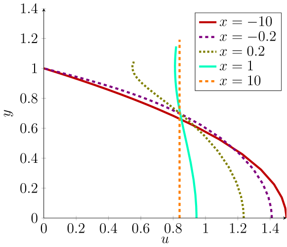
(a) Velocity component $u$ in cross stream direction.

(b) Velocity component $v$ in cross stream direction.

Figure 9: Velocity components in cross stream direction at inflow ($x=-10$), near the die exit ($x=-0.2$, $x=-0.2$), further downstream in the free jet region $x=1$ and at outflow $x=10$.

Figure 9 shows the velocity components in the cross stream wise direction at inflow ($x=-10$), near the die exit ($x=-0.2$, $x=0.2$), further downstream in the free jet region $x=1$ and at outflow $x=10$. The velocity component $u$, is parabolic at inflow, shortly before the die exit ($x=-0.2$) the parabolic profile flattens inside the die, after the die exit the parabolic profile flattens further and builds a boundary layer in which it goes through a minimum $x=0.2$, then flattens increasingly until the plug flow value is reached. The vertical velocity component, which is zero at inflow, forms a parabolic-like profile with a small boundary layer near the die exit inside the die, which first sharpens shortly after exiting the die and then relaxes back to the zero value.

(a)
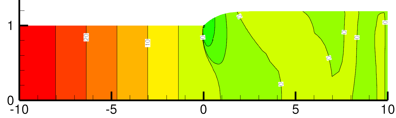
(b)
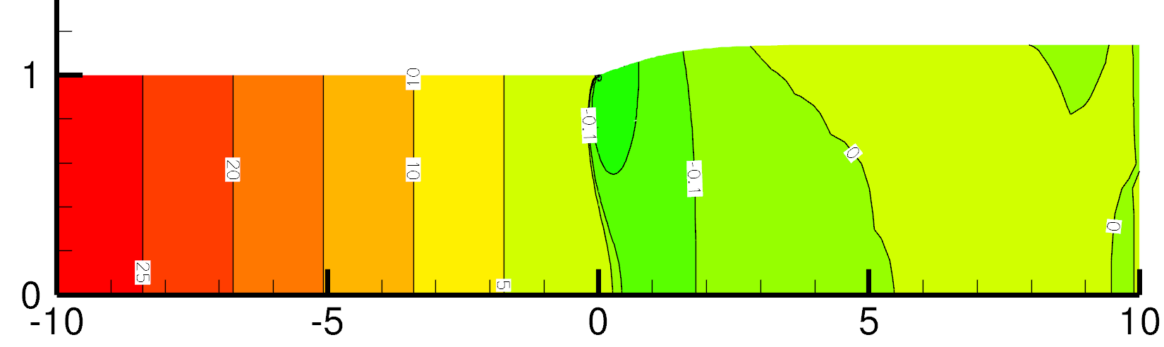
(c)
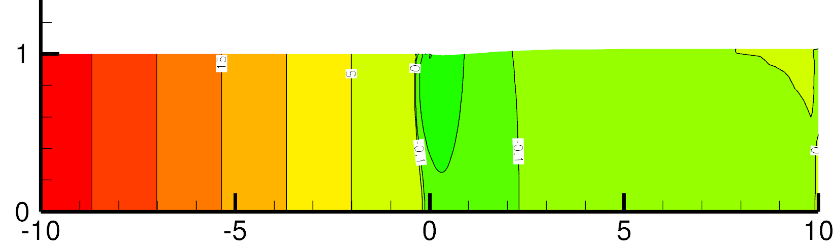
(d)
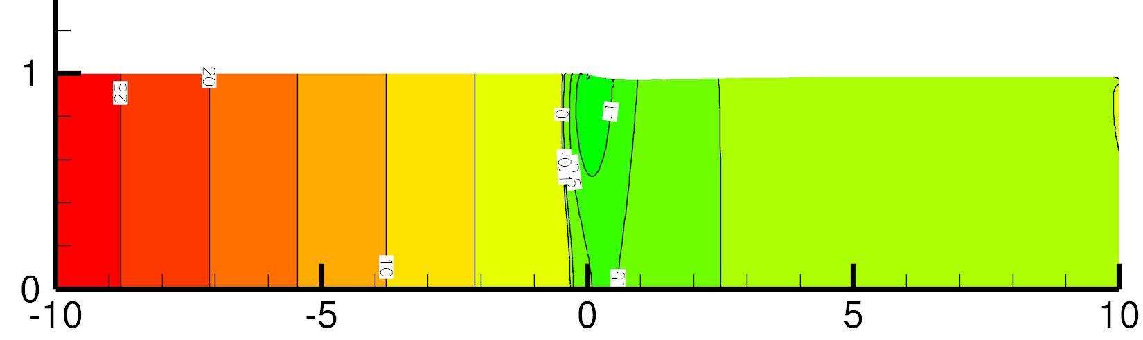
(e)

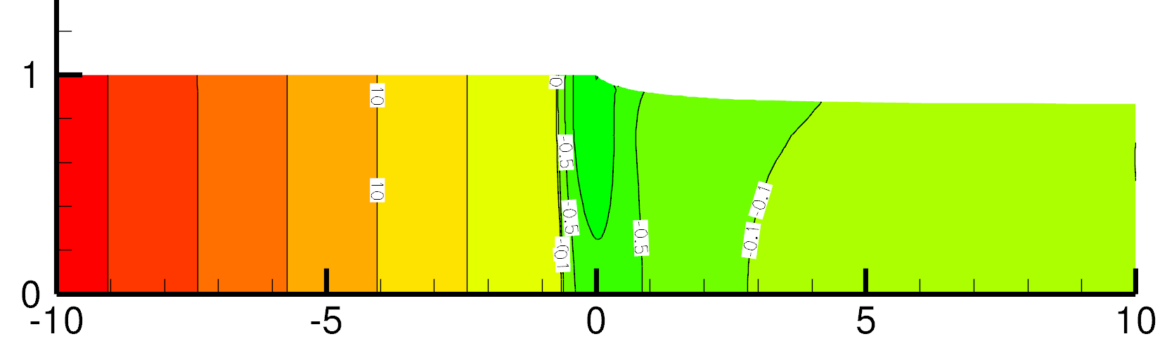
Figure 10: Pressure $p$ for $P=10$ for (a) $Re=0$, (b) $Re=3$, (c) $Re=7$, (d) $Re=10$ and (e) $Re=50$. Contours are indicated at intervals of $0.1$.

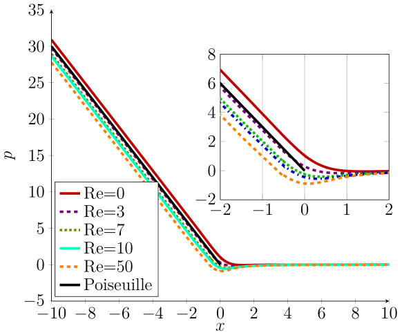
(a) Pressure $p$ along centreline.

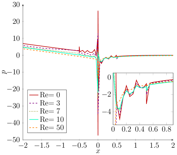
(b) Pressure $p$ around the singularity at the die exit.

Figure 11: Plots of pressure $p$ along LABEL:sub@subref:_centreline_newt_swell_p the centreline and LABEL:sub@subref:_fs_newt_swell_p_Re the wall and the free surface.

In the contour plots for the pressure $p$ displayed in Figure 10, we observe that the pressure isobars are curved near the die exit and in the free jet region into the downstream direction for low Reynolds number ($\text{Re}\,=0,3,7$) and into the upstream direction for higher Reynolds numbers ($\text{Re}\,>10$). The change in the pressure becomes more apparent when we explore the pressure values along the symmetry line (Figure 11a). Inside the die, the pressure gradient is constant as expected for Poiseuille flow. However, near the die exit ($x=0$) the pressure smoothly approaches zero for the plug flow. For higher Reynolds numbers the pressure on the centreline goes through a minimum. This behaviour of the pressure yields a shift in the pressure values at inflow, which is expressed by the pressure exit correction as defined in Equation (11).

4.4 Impact of slip

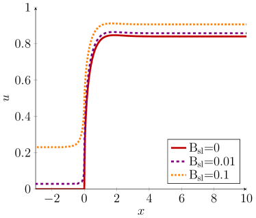
(a)

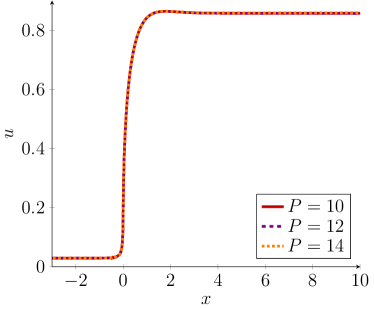
(b)

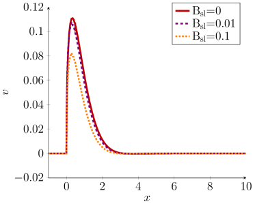
(c)

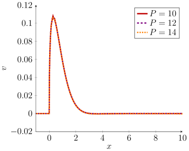
(d)

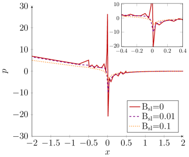
(e)

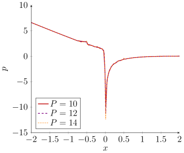
(f)

Figure 12: Dependence of LABEL:sub@subfig:_newton_swell_slip_fs_u velocity components $u$, LABEL:sub@subfig:_newton_swell_slip_fs_v $v$ and LABEL:sub@subfig:_newton_swell_slip_fs_p pressure on the slip parameter for $P=10$ and on mesh refinement for $B_{sl}=0.01$ (LABEL:sub@subfig:_newton_swell_slip_fs_u_P,LABEL:sub@subfig:_newton_swell_slip_fs_v_P,LABEL:sub@subfig:_newton_swell_slip_fs_p_P).

To alleviate the pressure singularity at the die exit, we investigate the effect of slip along the die wall on the dependent variables for $\text{Re}\,=0$. We therefore change the inflow profile according to Equation (16) and employ the slip condition (14) along the die wall. We explore the velocity field and the pressure along the free surface for slip parameter values of $B_{sl}=0.01$, $B_{sl}=0.1$ and $B_{sl}=0$ (no-slip) in Figure 12. With the introduction of slip along the wall, the horizontal velocity component experiences a smooth transition at the die exit in vast contrast to the kink at the singularity that is observed for the no-slip condition ($B_{sl}=0$) along the wall (Figure 12a). The change for the vertical velocity remains sudden and features a kink at the singularity. However, the maximum value of the vertical velocity component decreases with increasing slip (Figure 12c).

Table 4: Dependence of the swelling ratio on $P$ for $B_{sl}=0.1$ and $B_{sl}=0.01$.

$P$	$B_{sl}=0.1$	$B_{sl}=0.01$
10	1.1041	1.1671
12	1.1041	1.1673
14	1.1040	1.1670
Mitsoulis et al. (2012)	1.1041	1.1708

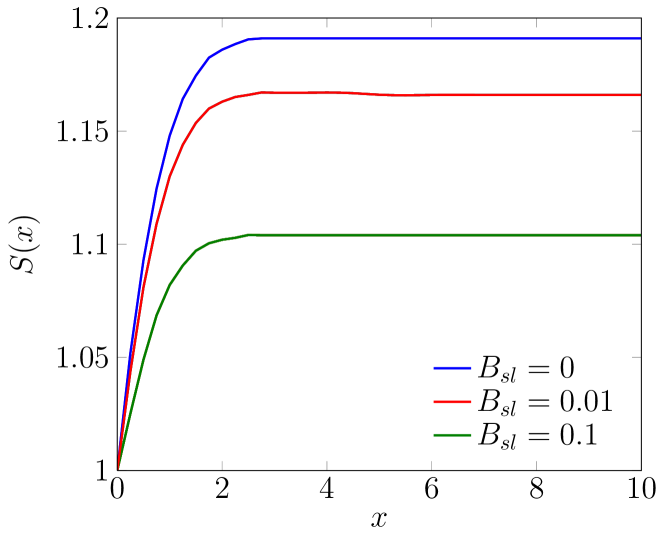
Figure 13: Free surface spline profile for increasing slip parameter.

The pressure profile at the singularity is changed drastically with slip along the wall and the Gibbs oscillations disappear (Figure 12e, LABEL:sub@subfig:_newton_swell_slip_fs_p_P). Even though the minimum of the pressure does not show a converging trend in the range of the employed polynomial orders, its value only increases slightly with increasing $P$ (Figure 12f). Table 4 lists the swelling ratios for increasing polynomial order, $P$, for $B_{sl}=0.1$ and $B_{sl}=0.01$. The swelling ratios are converged to three decimal places. Figure 12b and 12d show that the velocity values are converged for $P\geq 10$. The free surface spline for increasing slip parameter is shown in Figure 13. Increasing the slip parameter yields a decrease in swelling.

5 Conclusions

In this article, we have demonstrated the capabilities of the high-order spectral element method in the resolution of the stress singularity at the die exit in the plane Newtonian extrudate swell problem. We have shown that the spectral method approximates the infinite pressure value with exponentially increasing extreme values for increasing polynomial order. This high resolution approximation of the steep stress profiles yields excellent predictions of the swelling ratio. Our method predicts the same swelling ratio in comparison to low order finite element methods with significantly fewer number of degrees of freedom.

The only drawback of our high order method is the Gibbs oscillations, which appear in the vicinity of the singularity for the pressure approximation. These Gibbs oscillations are intrinsic to high order methods and they occur in the approximation of discontinuities or steep profiles. However, we have demonstrated that for the extrudate swell problem, the Gibbs oscillations stay confined to one element next to the singularity and their amplitude decreases significantly with increasing polynomial order. This small pollution in the pressure profile is the price to pay in the high order method for the otherwise excellent prediction of the steep pressure increase at the singularity.

We have given detailed results for a wide range of Reynolds numbers $0\leq\text{Re}\,\leq 100$ in terms of swell ratios, exit pressure losses, free surface profiles and velocity and pressure values. For the free surface profiles, we find three extrudate swell regimes. The first is a reduction in swelling ($\text{Re}\,\leq 6$), the second is a regime of a delayed swelling ($7\leq\text{Re}\,\leq 10$) and the third a contraction of the free liquid jet ($10<\text{Re}\,\leq 100$). With increasing Reynolds number the maximum pressure values decrease and the Gibbs oscillations decrease. We have then investigated the effect of slip along the die wall. We have observed a reduction of the swelling for different slip parameters $B_{sl}=\{0.01,0.1\}$ and have observed a drastic change in the pressure profile which showed no occurrence of Gibbs oscillations.

6 Acknowledgements

The authors wish to warmly thank Prof. Evan Mitsoulis for generously providing detailed data of his extrudate swell results. The first author would like to thank the UK Engineering and Physical Sciences Research Council for financial support.

References

- Ainsworth and Sherwin [1999] M. Ainsworth and S. Sherwin. Domain decomposition preconditioners for p and hp finite element approximation of Stokes’ equations. Comput. Meth. Appl. Mech. Eng., 175(3-4):243–266, 1999.
- Brezzi [1974] F. Brezzi. On the existence, uniqueness and approximation of saddle-point problems arising from Lagrangian multipliers. RAIRO Anal. Numér., 8:129–151, 1974.
- Choi and Hulsen [2011] Y.J. Choi and M.A. Hulsen. Simulation of extrudate swell using an extended finite element method. Korea-Aust Rheol J, 23(3):147–154, 2011.