One-Dimensional Coinless Quantum Walks

Abstract

A coinless, discrete-time quantum walk possesses a Hilbert space whose dimension is smaller compared to the widely-studied coined walk. Coined walks require the direct product of the site basis with the coin space, coinless walks operate purely in the site basis, which is clearly minimal. These coinless quantum walks have received considerable attention recently because they have evolution operators that can be obtained by a graphical method based on lattice tessellations and they have been shown to be as efficient as the best known coined walks when used as a quantum search algorithm. We argue that both formulations in their most general form are equivalent. In particular, we demonstrate how to transform the one-dimensional version of the coinless quantum walk into an equivalent extended coined version for a specific family of evolution operators. We present some of its basic, asymptotic features for the one-dimensional lattice with some examples of tessellations, and analyze the mixing time and limiting probability distributions on cycles.

I Introduction

The coined quantum walk (QW) on a line was introduced by Aharonov et al. Aharonov et al. (1993) and its generalization on regular graphs was studied in Ref. Aharonov et al. (2001). In this model, the particle hops from site to site depending on the value of an internal state of the walker, which plays the role of the coin. QWs on the line and on multi-dimensional lattices spread quadratically faster, in terms of the probability distribution, compared to the classical random walk model on the same underlying structure Aldous and Fill (200X). The coined model was successfully applied to develop quantum searching algorithms, especially for finding a marked node in graphs Shenvi et al. (2003); Ambainis et al. (2005); Portugal (2013). These searching algorithms generalize Grover’s algorithm in the sense that the data is distributed spatially and a price must be paid to go from one place to another when searching some item. The coined model in a regular graph of degree $d$ employs a $d$-dimensional unitary matrix that artificially enlarges the Hilbert space and thus, memory space, in any quantum computation. For non-regular graphs, the coined model requires different coins depending on the degree of the site.

The success of the coined model has stimulated the study of alternative QW models and a coinless version was introduced by Patel et al. Patel et al. (2005), and a coinless QW as a special case of a quantized cellular automaton even goes back to Meyer Meyer (1996). In Ref. Patel et al. (2005), the authors construct the propagator in terms of two non-commuting unitary matrices, motivated by the staggered fermion formalism of quantum field theories. It converts Dirac spinors used in continuous spacetime into spatial degrees of freedom on discrete lattices, amounting to a new version of QWs with no internal degree of freedom, i.e., no coin. The authors also applied their model to search a marked vertex in a two-dimensional lattice using numerical implementations Patel and Raghunathan (2012). Interestingly, the coinless model was rediscovered by Falk (Falk, 2013), who suggested a simple method of obtaining the two-stroke propagator without the internal degrees of freedom by spliting the vertices of the graph into disjoint patches that tessellate the two-dimensional lattice. His method can be readily used for other graphs, such as honeycombs and trees. Falk has also applied his model to search a marked vertex in the two-dimensional lattice using numerical implementations. A rigorous analytical proof based on an asymptotic analysis in terms of the system size, showing that the time complexity of Falk’s algorithm matches other QW models, appeared in Ref. Ambainis et al. (2013). The advantage of this model relies on using a smaller Hilbert space compared with other discrete time models. Recently, Ref. Childs and Ge (2014) used these ideas to improve the efficiency of searching algorithms based on continuous-time QW models Farhi and Gutmann (1998) for 2D-lattices. The coinless model may also provide an alternative that could be easier – or at least cheaper – to implement experimentally.

In this paper, we explore the one-dimensional versions of the coinless model for both, the infinite line and a finite-sized cycle. We present the coined and coinless models in a formalism that makes explicit the connection between these models. On the line we use the saddle-point method to obtain the asymptotic (large $t$) probability distribution. On the cycle, we obtain an explicit expression for the limiting probability distribution and present bounds for the mixing time ($\tau_{\epsilon}$). Our numerical analysis suggests that $\tau_{\epsilon}=\Theta(N/\epsilon)$, where $N$ is the number of vertices.

This paper is organized as follows. In Sec. II, we introduce the coinless and coined QW models on one-dimensional lattices. In Sec. III, we present an example of the equivalence of both versions. In Sec. IV, we present an abstract formulation that includes both QW models. In Sec. V, we present results for the one-dimensional coinless QW, such as its solution by Fourier analysis, the asymptotic form of its probability density function, the Anderson-like localization for a coinless 3-state QW, and for the cycle we obtain an analytical expression for the limiting probability distribution and bounds for the mixing time. In Sec. VII, we conclude with a discussion of the implications of our results.

II Typical formulations of Quantum Walks

The generic master-equation for any discrete-time quantum walk (DTQW),

$$\left|\Psi\left(t+1\right)\right\rangle={\cal U}\left|\Psi\left(t\right)\right\rangle,$$ (1)

with the time-evolution operator (or propagator) ${\cal U}$ is formally solved by $\left|\Psi\left(t\right)\right\rangle={\cal U}^{t}\left|\Psi\left(0\right)\right\rangle$. The Hilbert space of DTQW usually is a composite space which is spanned by the position states either augmented by coin states Aharonov et al. (2001) or augmented by an auxiliary space the dimension of which is the same of the original position space Szegedy (2004). At the end of the evolution, the extra space is traced out to generate information about the position of the walker. Locality is demanded in the sense that the walker does only short jumps around their original positions.

The smallest conceivable Hilbert space for such a system is spanned only by the site-basis $\left|\vec{n}\right\rangle$, also called the computational basis, similar to one used in the continuous-time QW model Farhi and Gutmann (1998). In such case, the state of the system can be described in terms of the site amplitudes $\psi_{\vec{x}}(t)=\left\langle\vec{x}|\Psi\left(t\right)\right\rangle$, i.e.,

$$\psi_{\vec{x}}(t+1)=\sum_{\vec{y}}\left\langle\vec{x}\right|{\cal U}\left|\vec{y}\right\rangle\psi_{\vec{y}}(t).$$ (2)

In a classical walk, the probability density function is simply given by $p_{\vec{x}}(t)=\psi_{\vec{x}}(t)$, but the fundamental difference of any QW derives from the fact that $\psi_{\vec{x}}(t)$ represents a complex site-amplitude from which the physical density is obtained via its modulus,

$$p_{\vec{x}}(t)=\left|\psi_{\vec{x}}(t)\right|^{2}=\left|\left\langle\vec{x}\right|{\cal U}^{t}\left|\Psi\left(0\right)\right\rangle\right|^{2}.$$ (3)

Eq. (3), by conservation of probability, implies that the evolution be unitary, and thus, reversible and volume-preserving, while the classical process is stochastic and irreversible and, hence, contractive. The modulus of a superposition of (complex) amplitudes, in contrast with the mere addition of positive weights classically, leads to a number of quantum effects, such as interference.

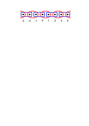
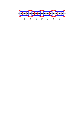
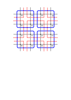
Figure 1: Depiction of tessellation options for reflection operators $U_{\vec{0},\vec{1}}$ in Eq. (4) in $D=1$ (left) and $D=2$ (right). Here, we use square blocks of length 2 in both dimensions (top left, and right). However, alternative (local) tessellations are conceivable, such as block-length 3, as shown for $D=1$ (bottom left), which lead to equally efficient QW. As a minimal requirement, at least the combination of both tessellations, needs to cover the lattice and both should be sufficiently overlapping.

II.1 Coinless Quantum Walk

Patel et.al. Patel et al. (2005) proposed a discrete-time quantum walk with no auxiliary space, which is called coinless or staggered QW. This model was re-invented in an alternative formulation in Ref. Falk (2013), which described an interesting method to generate this kind of QW in a 2D-lattice by partitioning it into disjoint patches that can be used to describe a reflection-based unitary operator called $U_{\vec{0}}$ (or ”even”) operator. The full evolution operator is obtained after building a second partition, which is analogous to the first one but diagonally shifted, generating a second reflection-based unitary operator called $U_{\vec{1}}$ (or ”odd”) operator that does not commute with $U_{\vec{0}}$. The resulting evolution operator then is ${\cal U}=U_{\vec{1}}U_{\vec{0}}$ . One can obtain classes of evolution operators by choosing creative graph tessellations that can considerably impact the effort needed to analyse the evolution.

Falk’s description can be generalized to a $D$-dimensional lattice where the two-stroke reflection propagator consists of

$$U_{\vec{0},\vec{1}}=2\sum_{\vec{x}}\left|u_{\vec{x}}^{\vec{0},\vec{1}}\right\rangle\left\langle u_{\vec{x}}^{\vec{0},\vec{1}}\right|-{\cal I},$$ (4)

where the sum extends over all lattice sites $\vec{x}$ that have, for $U_{\vec{0}}$, only even coordinates ($\vec{x}\equiv\vec{0}\mod 2$) or, for $U_{\vec{1}}$, only odd ones ($\vec{x}\equiv\vec{1}\mod 2$). Here, $\vec{0},\vec{1}$ refer to the binary vectors $\vec{0}=(0,\ldots,0)$ and $\vec{1}=(1,\ldots,1)$. The reflections $U_{\vec{0},\vec{1}}$ each mix the quantum state on hyper-square-blocks of $2^{D}$ sites that cover the lattice, as shown in Fig. 1. If we define $\vec{b}\in{\cal B}_{D}$, $0\leq b<2^{D}$, as that vector on the $D$-dimensional hypercube ${\cal B}_{D}$ whose components are the binary decomposition of the number $b$, we can write in general

$$\left|u_{\vec{x}}^{\vec{0},\vec{1}}\right\rangle=\sum_{\vec{b}\in{\cal B}_{D}}u_{\vec{b}}^{\vec{0},\vec{1}}\left|\vec{x}+\vec{b}\right\rangle,\quad\left(\vec{x}\equiv\vec{0},\vec{1}\mod 2\right),$$ (5)

with $\sum_{\vec{b}\in{\cal B}_{D}}\left|u_{\vec{b}}^{\vec{0},\vec{1}}\right|^{2}=1$, which is a generalization of the operators introduced by Falk for $D=2$ and restricted to uniform $u_{\vec{b}}^{\vec{0},\vec{1}}=\frac{1}{2}$. The interlacing of $U_{\vec{0}}$ and $U_{\vec{1}}$ in the time evolution ${\cal U}^{t}\left|\Psi\left(0\right)\right\rangle$ spreads the QW between diagonally offset, overlapping sets of blocks. Falk has numerically analyzed the efficiency of a search algorithm based on the two-dimensional version of this model. Ref. Ambainis et al. (2013) rigorously proved that the efficiency of Falk’s algorithm matches other models of QWs.

As the most tractable case, we consider here the coinless QW on the line, $D=1$, with the generalized form in Eq. (5), allowing for a tunable family of parameters $\alpha,\beta,\phi_{1},\phi_{2}$ for the block-states:

$$\left|u_{x}^{{0}}\right\rangle = \cos\frac{\alpha}{2}\left|2x\right\rangle+\textrm{e}^{i\phi_{1}}\sin\frac{\alpha}{2}\left|2x+1\right\rangle,$$ (6)

$$\left|u_{x}^{{1}}\right\rangle = \sin\frac{\beta}{2}\left|2x+1\right\rangle+\textrm{e}^{i\phi_{2}}\cos\frac{\beta}{2}\left|2x+2\right\rangle.$$ (7)

Here, $\left|u_{x}^{{0,1}}\right\rangle$ each cover blocks of merely two sites and the propagator is ${\cal U}=U_{\textrm{1}}U_{\textrm{0}}$, where

$$U_{\textrm{0,1}}=2\,\sum_{x=-\infty}^{\infty}{\left|{u^{\textrm{0,1}}_{x}}\right\rangle}{\left\langle{u^{\textrm{0,1}}_{x}}\right|}-{\cal I}.$$ (8)

It is now straightforward to calculate the matrix $\left\langle x\left|{\cal U}\right|y\right\rangle$ for the propagator ${\cal U}$ in the site basis by inserting Eqs. (6) and (7). Using

$$\left\langle x\biggm{|}u_{y}^{{0}}\right\rangle = \cos\frac{\alpha}{2}\,\delta_{x,2y}+\textrm{e}^{i\phi_{1}}\sin\frac{\alpha}{2}\,\delta_{x,2y+1},$$ (9)

$$\left\langle x\biggm{|}u_{y}^{{1}}\right\rangle = \sin\frac{\beta}{2}\,\delta_{x,2y+1}+\textrm{e}^{i\phi_{2}}\cos\frac{\beta}{2}\,\delta_{x,2y+2},$$

and

$$\left\langle u_{x}^{{1}}\biggm{|}u_{y}^{{0}}\right\rangle=\textrm{e}^{i\phi_{1}}\sin\frac{\alpha}{2}\sin\frac{\beta}{2}\,\delta_{x,y}+\textrm{e}^{-i\phi_{2}}\cos\frac{\alpha}{2}\cos\frac{\beta}{2}\,\delta_{x+1,y},$$

to calculate $\left\langle 2x\left|{\cal U}\right|y\right\rangle$ and $\left\langle 2x+1\left|{\cal U}\right|y\right\rangle$, we obtain for the evolution equations

$$\psi_{2x}(t+1) = \sin\alpha\sin\beta\,\textrm{e}^{i(\phi_{1}+\phi_{2})}\psi_{2x-2}(t)-\cos\alpha\sin\beta\,\textrm{e}^{i\phi_{2}}\psi_{2x-1}(t)-$$ (10)

$$\cos\alpha\cos\beta\,\psi_{2x}(t)-\sin\alpha\cos\beta\,\textrm{e}^{-i\phi_{1}}\psi_{2x+1}(t),$$

$$\psi_{2x+1}(t+1) = \sin\alpha\cos\beta\,\textrm{e}^{i\phi_{1}}\psi_{2x}(t)-\cos\alpha\cos\beta\,\psi_{2x+1}(t)+$$ (11)

$$\cos\alpha\sin\beta\,\textrm{e}^{-i\phi_{2}}\psi_{2x+2}(t)+\sin\alpha\sin\beta\,\textrm{e}^{-i(\phi_{1}+\phi_{2})}\psi_{2x+3}(t).$$

II.2 Coined Quantum Walk

Due to its importance for quantum search algorithms, the most studied formulation of a discrete-time QW proceeds by introducing a quantum coin. In a coined QW, the time-evolution operator takes the form

$${\cal U}={\cal S}\left({\cal C}\otimes{\cal I}\right),$$ (12)

containing the “shift” operator ${\cal S}$ and the quantum coin ${\cal C}$. Like the Bernoulli coin used to drive a classical random walk, ${\cal C}$ is meant to determine which share of every on-site amplitude gets transported to each of the neighboring sites. To preserve unitarity, ${\cal C}$ is usually conceived of as a unitary operator of a rank commensurate with the neighborhood degree $d$ of the site, whose application entangles a $d$-dimensional vector of site amplitudes $\psi_{\vec{x}}(t)$ before the shift-operator ${\cal S}$ distributes those amplitudes at each site to its respective neighboring sites.

Such a coined QW possesses great conceptual clarity, and has been shown to lead to the best-known efficiency for low-dimensional ($D\leq 3$) quantum search algorithms. However, the requirement to match the coin-space to the neighborhood degree is not only a severe limitation to regular lattices, but especially burdens the formulation with a Hilbert space that is now the product of coin and site-space.

As a concrete example, let us discuss the nearest-neighbor QW on a line, which only requires a unitary coin matrix of rank $d=2$, in its most general form given by

$${\cal C}=\left(\begin{array}[]{cc}\cos\rho&\sin\rho\,{\textrm{e}}^{i\theta}\\ \sin\rho\,{\textrm{e}}^{i\varphi}&-\cos\rho\,{\textrm{e}}^{i\left(\theta+\varphi\right)}\end{array}\right)$$ (13)

in terms of three real parameters ($\rho,\theta,\varphi$). It is conventional to expand the solutions in the coin- and the site basis $\left|s\right\rangle\otimes\left|x\right\rangle=\left|s,x\right\rangle$, where $s=0,1$ refers to the two directions out of each site, and $x$ labels the sites on the line. The most general form of ${\cal U}$ on the 1D-line is then

$${\cal U} = \sum_{x}\sum_{\mu,\nu=0}^{1}\left\{A_{\mu,\nu}\left|\mu,x+1\right\rangle\left\langle\nu,x\right|+B_{\mu,\nu}\left|\mu,x-1\right\rangle\left\langle\nu,x\right|\right\},$$ (14)

with matrices $A=P{\cal C}$ and $B=Q{\cal C}$, where

$$P=\left(\begin{array}[]{cc}1&0\\ 0&0\end{array}\right),\quad Q=\left(\begin{array}[]{cc}0&0\\ 0&1\end{array}\right),$$ (15)

in a commonly used (but restrictive) interpretation of the shift operator at each site. Taking, say, $\theta=\frac{\pi}{2}$ and $\varphi=0$ in Eq. (13), we get for the evolution equations in (2) for the upper and lower component $\psi_{x}^{(0,1)}(t)$ of the wave function:

$$\psi_{x}^{(0)}(t+1) = \cos\rho\,\psi_{x+1}^{(0)}(t)-\sin\rho\,\psi_{x+1}^{(1)}(t),$$

$$\psi_{x}^{(1)}(t+1) = \sin\rho\,\psi_{x-1}^{(0)}(t)+\cos\rho\,\psi_{x-1}^{(1)}(t).$$ (16)

These, or similar systems, have been studied at great length (Ambainis et al., 2001; Bach et al., 2004; Portugal, 2013). Occasionally, a coined QW with the possibility to remain at the same site is considered, leading to a three-term propagator in Eq. (14) (Inui and Konno, 2005; Falkner and Boettcher, 2014). However, in this formulation, such a walk already requires a coin of rank $d=3$.

III Relation between Coinless and Coined Quantum Walk on a Line

The coinless evolution equations (10) and (11) can be rewritten as two-dimensional vectors:

$$\left[\begin{array}[]{c}\psi_{2x}(t+1)\\ \psi_{2x+1}(t+1)\end{array}\right] = A\left[\begin{array}[]{c}\psi_{2x-2}(t)\\ \psi_{2x-1}(t)\end{array}\right]+M\left[\begin{array}[]{c}\psi_{2x}(t)\\ \psi_{2x+1}(t)\end{array}\right]+B\left[\begin{array}[]{c}\psi_{2x+2}(t)\\ \psi_{2x+3}(t)\end{array}\right],$$ (25)

where we set

$$A=\sin\beta\,{\textrm{e}^{i(\phi_{1}+\phi_{2})}}P{\cal C},\quad B=\sin\beta\,{\textrm{e}^{i(\phi_{1}+\phi_{2})}}Q{\cal C}\quad M=\cos\beta\,{\textrm{e}^{i(\phi_{1}+\phi_{2})}}R{\cal C}$$ (26)

with $R=\left[\begin{array}[]{cc}0&-{\textrm{e}^{i\phi_{2}}}\\ {\textrm{e}^{-i\phi_{2}}}&0\end{array}\right]$ and $P,Q$ as in Eq. (15), and the coin ${\cal C}$ in Eq. (13) for $\rho=\frac{\pi}{2}-\alpha$, $\theta=\pi-\phi_{1}$ and $\varphi=-(\phi_{1}+2\phi_{2})$.

We note that these equations are very similar to those for the coined QW in Eq. (16), if we reinterpret consecutive pairs of an even site and the odd site to its right into a single node by treating the two original sites as upper and lower coin states, respectively. This mapping is exact only for $\beta=\frac{\pi}{2}$, for which the self-term with $M$ in Eq. (25) disappears. For other values of $\beta$, we require a generalized interpretation of the shift operators. This corresponds to the symmetric choice for $\left|u_{x}^{{1}}\right\rangle$ in Eq. (7), however, the equally symmetric choice of $\alpha=\frac{\pi}{2}$ for $\left|u_{x}^{{0}}\right\rangle$ provides only a degenerate, one-sided QW with ${\cal C}\to{\cal I}$. The equivalent of the Hadamard QW would only emerge for the choice $\alpha=\frac{\pi}{4}$, since Eq. (25) is formally equivalent to Eq. (16) when $\rho=\frac{\pi}{4}$. Still, it is remarkable that the meaning of the two reflection operators $U_{0}$ and $U_{1}$ of the coinless QW in Eq. (8) in this case can be related to corresponding sequence of applying coin ${\cal C}$ and shift operator ${\cal S}$ in the coined QW. In general, however, the possibilities of the definition for the coinless QW in Eqs. (6) and (7) exceed those provided for by the conventional coined QW as presented in Sec. II.2. We therefore provide an abstract formulation that unifies both, coined and coinless QW, in a more general framework.

IV Generalized Quantum Walks

As the preceding discussion shows, the coined and coinless QW possess very similar structures. The sequence of coin and shift operation closely resembles the action of the two-stroke reflection operator. Yet, each already presents a very specific choice of operations (shifts, reflections, etc) that are suggested by their intuitive nature for their respective situations. Due to those restrictions, their equivalence can be shown only under certain circumstances, as we have discussed in Sec. III. Removing those restrictions reveals a more general equivalence, which we explore in the following.

The master equation, Eq. (1), merely imposes unitartity, however, to obtain a physical walk we also demand locality over a bounded neighborhood (i.e., a sparse adjacency matrix), which we here simply take as nearest-neighbor exchanges. We then define on a $d$-regular network, such as a lattice with $d=2D$, the propagator

$${\cal U} = \sum_{\vec{n}}^{{\cal N}/r}\left\{M\left|\vec{n}\right\rangle\left\langle\vec{n}\right|+\sum_{\mu=1}^{d}A_{\mu}\left|\vec{n}\right\rangle\left\langle\vec{n}+\vec{e}_{\mu}\right|\right\},$$ (27)

over a partial basis $\left\{\left|\vec{n}\right\rangle\right\}$ of size ${\cal N}/r$ in the Hilbert space of rank ${\cal N}$. $A_{\mu}$ or $M$ are operators of rank $r$ that determine the portion of the wave function at site $\vec{n}$ that either gets transported to one of $d$ neighboring site $\vec{n}+\vec{e}_{\mu}$ or remains at the site during the next update, respectively. Here, it could be ${\cal N}=rN$ for the product of rank-$r$ coin and site space in the coined QW with $\vec{n}$ denoting all sites. Alternatively, ${\cal N}=N$ and the ${\cal N}/r$ subset of sites $\vec{n}$ labels blocks possessing $r$ block-internal sites, such as in Eq. (5), each in some tessellation of the network in the coinless QW. In that case, $M$ entangles those $r$ sites in each block anckered at $\vec{n}$, while the $A_{\mu}$ transfers amplitudes to the $d$ adjacent blocks labeled by $\vec{n}+\vec{e}_{\mu}$. For our one-dimensional example in Sec. II, the former leads to evolution equations such as in (16), while the latter leads to Eq. (25). Note that in Eq. (27) we required a certain level of (i) homogeneity (in that each block has the same operators $M,A_{\mu}$ and hence the same number of adjacent blocks, $d$), and (ii) reciprocity (in that there exist pairs $\mu,\nu=\nu\left(\mu\right)$ such that for every two adjacent blocks $\vec{n},\vec{m}$ with $\vec{n}+\vec{e}_{\mu}=\vec{m}$ it is also $\vec{m}+\vec{e}_{\nu}=\vec{n}$). Both conditions are obvious on a uniform $D$-dimensional rectangular lattice with $r=d=2D$ neighboring blocks, where simply $\vec{e}_{\nu}=-\vec{e}_{\mu}$ for each direction, but requires some thought for more general networks.

Using Eq. (27) and expanding ${\cal U}^{\dagger}{\cal U}$, the unitarity conditions implies that

$${\cal I}_{r} = M^{\dagger}M+\sum_{\mu=1}^{d}A_{\mu}^{\dagger}A_{\mu},$$

$$0 = A_{\mu}^{\dagger}M+M^{\dagger}A_{\nu\left(\mu\right)},\quad\left(1\leq\mu\leq d\right)$$

$$0 = A_{\mu}^{\dagger}A_{\nu},\quad\left(1\leq\mu,\nu\leq d,\mu\not=\nu\right),$$ (28)

which implies that $M+\sum_{\mu=1}^{d}A_{\mu}$ must be unitary. These conditions can not be satisfies in general by scalars, except for trivial cases. Thus, similar in spirit to Dirac’s derivation of relativistic QM, this algebra requires matrix respresentations of the hopping operators and multi-component spinors to represent states.

One specific representation is provided by $r$-dimensional hopping matrices with $r\geq d$ that arise from the combination of coin- and shift matrices, such as for the line in Eq. (14), with ${\cal N}=Nr$. Another specific representation results from the combination of operators, as those in Eq.  (8), in the coinless case that lead to relations between neighboring sites on a patch, such as Eqs. (25-26) for the coinless QW on the line. The latter has the apparent advantage that site-space and Hilbert space coincide, ${\cal N}=N$, however, every site within a patch of size $r$ requires a separate considertion. As we will see in Sec. V, for example, the coinless walk on a line requires a Fourier analysis that is staggered between even and odd sites for $r=d=2$.

More general choices are possible than the traditional coined walk, with specific shift operators for the transfer of a single component of the wave-function along a lattice direction, or the reflection operators for our coinless QW. Also, the algebra in Eq. (28) can also be satisfied by a higher-dimensional vector space than the degree imposed by the network, $r\geq d$. We have not tried here to enumerate systematically the most general choice even for the simple line, as most would likely not lead to any new phenomena. Note, however, that already adding a third component to the QW ($r=3$) on the line ($d=2D=2$), coined (Inui and Konno, 2005; Falkner and Boettcher, 2014) or coinless (see Sec. V.3 below), allows for localization effects that do not exist for any two-dimensional operators.

V Results for Coinless Quantum Walks on a Line

In this Section, we list a few equivalent results for properties of the one-dimensional coinless QW that mirror those that have been found important for the understanding of a coined QW. First, we provide explicit results for the wave-function on even and odd sites of the infinite line as Fourier integrals. From these, we determine the asymptotic probability density function (PDF). We also discuss alternative tessellations, involving three sites simultaneously, that are equivalent to the behavior for a three-state coined QW, but seem to exhibit a more varied localization property. In the next Section, we consider the coinless QW on a finite-length cycle, and use its solution to provide bounds on the mixing time.

V.1 Fourier Solution on the Infinite Line

We define as a Fourier transform, staggered between even and odd sites, the vectors

$${\left|{\tilde{\psi}_{k}^{\textrm{0}}}\right\rangle} = \sum_{x=-\infty}^{\infty}\textrm{e}^{-2xki}{\left|{2x}\right\rangle},$$ (29)

$${\left|{\tilde{\psi}_{k}^{\textrm{1}}}\right\rangle} = \sum_{x=-\infty}^{\infty}\textrm{e}^{-(2x+1)ki}{\left|{2x+1}\right\rangle},$$ (30)

where $k\in[-\pi,\pi]$. For a fixed $k$, they define a plane that is invariant under the action of the evolution operator. The analysis of the dynamics can be reduced to a two-dimensional subspace of ${\cal H}$ by defining a reduced evolution operator

$$U_{\textrm{RED}}^{(k)}=\left[\begin{array}[]{cc}A&-B^{*}\\ B&A^{*}\end{array}\right],$$ (31)

where

$$A = -\cos\alpha\cos\beta+\sin\alpha\sin\beta\,\textrm{e}^{i(\phi_{1}+\phi_{2})}\textrm{e}^{2ki},$$ (32)

$$B = \sin\alpha\cos\beta\,\textrm{e}^{i\phi_{1}}\textrm{e}^{ki}+\cos\alpha\sin\beta\,\textrm{e}^{-i\phi_{2}}\textrm{e}^{-ki}.$$ (33)

$U_{\textrm{RED}}^{(k)}$ is unitary because $A\,A^{*}+B\,B^{*}=1.$ The eigenvalues are $\lambda=\textrm{e}^{\pm i\theta}$ and can be obtained from the characteristic polynomial, which is ${\lambda}^{2}-(A+A^{*})\lambda+1.$ Then

$$\cos\theta=\frac{A+A^{*}}{2}.$$ (34)

The quantities defined in these expressions depend on $k$ and others parameters. We will make explicit those parameters only in some equations.

There are trivial solutions that are obtained by taking either $A=0$ or $B=0$. $U_{\textrm{RED}}^{(k)}$ in the latter case is diagonal and the wave function moves to right or to the left without spreading. On the other hand, if $A=0$, the wave function oscillates back and forth without spreading. The first case is obtained when $(\alpha,\beta)=(0,0)$, $(\pi/2,\pi/2)$ or by adding any multiple of $\pi$ to $\alpha$ or $\beta$; and the second case when $(\alpha,\beta)=(0,\pi/2)$ or by adding any multiple of $\pi$. In any of those cases, the eigenvalues of the evolution operator is evenly spread out on the unit complex circle.

The non-trivial eigenvectors of $U_{\textrm{RED}}^{(k)}$ are

$$\frac{1}{\sqrt{C^{\pm}}}\left(\begin{array}[]{c}-B^{*}\\ \textrm{e}^{\pm i\theta}-A\end{array}\right),$$ (35)

where

$$C^{\pm}=\sin\theta\,\big{(}2\sin\theta\pm i\,(A-A^{*})\big{)}.$$ (36)

There are special values of $k$ such that $C^{\pm}=0$. They are: 1) $\alpha=\beta$ and $\phi_{1}+\phi_{2}+2k=\pm\pi$, 2) $\alpha+\beta=\pi$ and $\phi_{1}+\phi_{2}+2k=0,\pm 2\pi$. In those cases, we have to take the limit of eigenvectors (35) when $k$ approach to the troublesome values.

The eigenvectors of the full propagator $U$ associated with eigenvalues $\textrm{e}^{\pm i\theta}$ are

$${\left|{v_{k}^{\pm}}\right\rangle}=\frac{1}{\sqrt{C^{\pm}}}\left(-B^{*}{\left|{\tilde{\psi}_{k}^{\textrm{0}}}\right\rangle}+(\textrm{e}^{\pm i\theta}-A){\left|{\tilde{\psi}_{k}^{\textrm{1}}}\right\rangle}\right),$$ (37)

and we can write

$$U=\int_{-\pi}^{\pi}\frac{\textrm{d}k}{2\pi}\left(\textrm{e}^{i\theta}{\left|{v_{k}^{+}}\right\rangle}{\left\langle{v_{k}^{+}}\right|}+\textrm{e}^{-i\theta}{\left|{v_{k}^{-}}\right\rangle}{\left\langle{v_{k}^{-}}\right|}\right).$$ (38)

If we take ${\left|{\psi(0)}\right\rangle}={\left|{0}\right\rangle}$ as initial condition, the walker’s state at time $t$ is

$${\left|{\psi(t)}\right\rangle} = \sum_{x=-\infty}^{\infty}\left(\psi_{2x}(t)\,{\left|{2x}\right\rangle}+\psi_{2x+1}(t)\,{\left|{2x+1}\right\rangle}\right),$$ (39)

where

$$\psi_{2x}(t)=\int_{-\pi}^{\pi}\frac{\textrm{d}k}{2\pi}\,|B|^{2}\left(\frac{\textrm{e}^{i(\theta t-2kx)}}{C^{+}}+\frac{\textrm{e}^{-i(\theta t+2kx)}}{C^{-}}\right)$$ (40)

and

$$\psi_{2x+1}(t)=\int_{-\pi}^{\pi}\frac{\textrm{d}k}{2\pi}\,\frac{B\sin\theta t}{\sin\theta}\,\textrm{e}^{-(2x+1)ki}.$$ (41)

The probability distribution is obtained after calculating $p_{2x}(t)=\left|\psi_{2x}(t)\right|^{2}$ and $p_{2x+1}(t)=\left|\psi_{2x+1}(t)\right|^{2}$. In the next Section, we use the saddle-point expansion method to obtain an asymptotic expression for the probability distribution. The probability distribution is not symmetric in this case. An alternative initial condition which yields a symmetric QW is $({\left|{0}\right\rangle}+i{\left|{1}\right\rangle})/2$.

V.2 Asymptotic PDF of a coinless Quantum Walk

The probability density function (PDF) $p_{{x}}(t)$ for a walker to be at a site ${x}$ at time $t$ provides the most comprehensive description of any QW. All of its properties, such as the mean-square displacement or first-return probabilities, derive from the PDF, making it the central object of any textbook discussion of classical random walks (Itzykson and Drouffe, 1989; Redner, 2001) and transport processes (Weiss, 1994). This also holds for QWs (Portugal, 2013; Venegas-Andraca, 2012).

Starting from Eq. (40) [or, equivalently, Eq. (41)], we define an effective Hamiltonian,

$${\cal H}_{\pm}\left(k\right)=-2vk\pm\theta(k),$$ (42)

and pursue a stationary-phase solution for $t\gg 1$ (Bender and Orszag, 1978) via $\frac{\partial}{\partial k}{\cal H}_{\pm}\left(k_{\pm}\right)=0$, i.e.,

$$v=\frac{x}{2t}=\pm\frac{1}{2}\frac{\partial\theta\big{(}k_{\pm}\big{)}}{\partial k}.$$ (43)

Note that it is convenient to introduce the maximal speed $2$, such that the effective velocity $|v|<1$ is gauged in these units, obtained from the furthest reach in a given tessellation of a single application of $U$, which here is uniformly the side-length of a 2-block. Finally, expanding ${\cal H}_{\pm}\left(k\right)\sim{\cal H}_{\pm}\left(k_{\pm}\right)+\frac{1}{2}{\cal H}_{\pm}^{\prime\prime}\left(k_{\pm}\right)\left(k-k_{\pm}\right)^{2}$ and substituting $k=k_{\pm}+(\pm 1+i)u$, with $u$ as the new integration variable, allows the asymptotic evaluation of the integral in Eqs. (40) and (41) as a Gaussian along a complex contour.

For example, for $\alpha+\beta=\pi$ and defining the “effective” velocity $v_{0}=\sin\alpha$, i.e., $\theta_{\pm}(k)=\mp\arccos\left(1-2v_{0}^{2}\sin^{2}k\right)$ from Eq. (34), we find the solutions of Eq. (43)

$$k_{\pm}=\arccos\left[\pm\frac{v}{v_{0}}\sqrt{\frac{1-v_{0}^{2}}{1-v^{2}}}\right],$$ (44)

which are valid only for $\left|v\right|<v_{0}$. Hence, only for $\alpha=\beta=\frac{\pi}{2}$, i.e., uniform $u_{x}^{\vec{0},\vec{1}}=\frac{1}{\sqrt{2}}$ in Eq. (5), can the 1D-QW reach maximal speed $c$, however, at that point the walk degenerates into one-sided lockstep motion. At $k_{\pm}$, we find

$${\cal H}_{\pm}=2vk_{\pm}\mp\arccos\left[\frac{1+v^{2}-2v_{0}^{2}}{1-v^{2}}\right],$$ (45)

and

$$\left|{\cal H}_{\pm}^{\prime\prime}\left(k_{\pm}\right)\right|=\left(1-v^{2}\right)\sqrt{\frac{v_{0}^{2}-v^{2}}{1-v_{0}^{2}}}.$$ (46)

Replacing the values for $k_{\pm}$ into the expressions $|B|^{2}/C^{\pm}$ inside the integrals (40) and (41), working out all cases we eventually find for Eq. (3) for odd sites:

$$p_{2x+1}(t)\sim\frac{1}{\pi}\,\sqrt{\frac{1-v_{0}^{2}}{v_{0}^{2}-v^{2}}}\,\cos^{2}\left\{\frac{\pi}{4}+t\,{\cal H}_{\pm}\big{(}k_{\pm}\big{)}\right\}$$ (47)

and $p_{2x}(t)\sim\frac{1+v}{\left(1-v\right)}p_{2x+1}(t)$ for $\left|v\right|<v_{0}<1$ at $t\gg 1$. We plot the resulting PDF as $p_{\vec{x}}(t)=\left(p_{2x}(t)+p_{2x+1}(t)\right)/2$ in Fig. 2 and compare it with exact simulations. Note the asymmetry of the PDF; for $v_{0}\to 1$ ($\alpha\to\pi/2$) it degenerates into $\rho(v)\to\delta\left(v_{0}\mp v\right)$ for $\left|\Psi\left(0\right)\right\rangle=\left|0\right\rangle$.

In the $2D$ case, the real eigenvalues of the reduced propagator produce a motionless delta spike at the origin generating Anderson localizations, similar to the ones that have been noticed on the coined QW model (Inui and Konno, 2005; Falkner and Boettcher, 2014). The $1D$ case analyzed in this paper has no static localization and the reduced propagator does not have real (unit) eigenvalues, except for trivial limiting cases. An easy way to introduce localization in $1D$ coined QWs is by enlarging the coin space, see for example the models addressed in (Inui and Konno, 2005; Falkner and Boettcher, 2014) and our discussion in Sec. V.3. In the tessellation model, it seems that the blocks need to have at least three sites in order to produce localization.

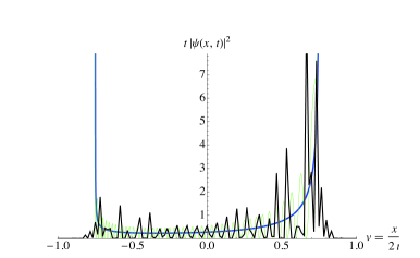
Figure 2: Plot of the rescaled PDF $tp_{x}(t)\sim\rho\left(v\right)$ at $t=30$ in the scaling variable $v=\frac{x}{2t}$ for the coinless QW in $D=1$ at $\alpha+\beta=\pi$ and $v_{0}=\sin\alpha=\frac{3}{4}$, initiated at $t=0$ on site $x=0$, $\left|\Psi\left(0\right)\right\rangle=\left|0\right\rangle$. The simulation (dark line) contains some more structure than the full asymptotic form (green shaded line) from Eq. (47) can represent at $t=30$. The envelope function (thickened blue line), also obtained from Eq. (47) by removing the explicitly $t$-dependent phase, represents the average behavior and eccentricity of the exact data quite well, within the range of its validity bracketed by poles at $v=\pm v_{0}$.

V.3 A coinless 3-state QW

Here, we reconsider a one-dimensional coinless QW for the tessellation shown on the bottom-left of Fig. 1. This form has a few interesting new features not previously considered for a coinless QW: (i) It can be shown that every pair of reflection operators generically leads to localization. (ii) In this tessellation, neither set of blocks, for the first nor the second reflection operator, completely covers the lattice individually, however, the combination of both sets of blocks do, and they have an overlap that is symmetric and reaches every part of the lattice.

For consistency in the notation with Eq. (4), we define the evolution operator as ${\cal U}=U_{1}U_{0}$ with the two reflection operators as

$$U_{0,1}=2\sum_{x=0}^{\infty}\left|u_{x}^{0,1}\right\rangle\left\langle u_{x}^{0,1}\right|-{\cal I},$$ (48)

with

$$\left|u_{x}^{\textrm{0}}\right\rangle = \frac{1}{\sqrt{3}}\left(\left|4x-1\right\rangle+\left|4x\right\rangle+\left|4x+1\right\rangle\right),$$ (49)

$$\left|u_{x}^{\textrm{1}}\right\rangle = \frac{1}{\sqrt{3}}\left(\left|4x+1\right\rangle+\left|4x+2\right\rangle+\left|4x+3\right\rangle\right).$$ (50)

The staggered Fourier basis is spanned by four vectors

$${\left|{\tilde{\psi}_{k}^{j}}\right\rangle}=\sum_{x=-\infty}^{\infty}\textrm{e}^{-(4x+j)ki}{\left|{2x+j}\right\rangle},$$ (51)

where $0\leq j\leq 3$. The four-dimensional space spanned by those vectors is invariant under the action of the evolution operator and allows to use a reduced evolution operator given by

$$U_{\textrm{RED}}=\frac{1}{9}\left[\begin{array}[]{cccc}3&-6\,{{\rm e}^{-ik}}&0&-6\,{{\rm e}^{ik}}\\ \vskip 6.0pt plus 2.0pt minus 2.0pt\cr 4\,{{\rm e}^{-3ik}}-2\,{{\rm e}^{ik}}&4\,{{\rm e}^{-4ik}}+1&-6\,{{\rm e}^{-ik}}&-2\,{{\rm e}^{-2ik}}-2\,{{\rm e}^{2ik}}\\ \vskip 6.0pt plus 2.0pt minus 2.0pt\cr 4\,{{\rm e}^{-2ik}}+4\,{{\rm e}^{2ik}}&4\,{{\rm e}^{-3ik}}-2\,{{\rm e}^{ik}}&3&-2\,{{\rm e}^{-ik}}+4\,{{\rm e}^{3ik}}\\ \vskip 6.0pt plus 2.0pt minus 2.0pt\cr-2\,{{\rm e}^{-ik}}+4\,{{\rm e}^{3ik}}&-2\,{{\rm e}^{-2ik}}-2\,{{\rm e}^{2ik}}&-6\,{{\rm e}^{ik}}&1+4\,{{\rm e}^{4ik}}\end{array}\right],$$ (52)

such that

$${\cal U}\,{\left|{\tilde{\psi}_{k}^{j}}\right\rangle}=\sum_{l=0}^{3}\left\langle l\left|U_{\textrm{RED}}\right|j\right\rangle{\left|{\tilde{\psi}_{k}^{j}}\right\rangle}.$$ (53)

The eigenvalues of $U_{\textrm{RED}}$ are 1 with multiplicity 2 and $\textrm{e}^{\pm i\theta}$, where

$$\cos\theta=\frac{1}{9}\left(4\cos 4k-5\right).$$ (54)

The fact that $U_{\textrm{RED}}$ has eigenvalue 1 (which does not depend on $k$) implies that this QW has localization, that is, part of the wave function does not move. Fig. 3 shows the probability distribution of the walk after 20 steps with initial state located at $x=0$. The sharp peak at the origin does not move and is always present there regardless the number of steps. This is in contrast to the coined 3-state walk, where there is no localization for the Fourier coin, for example.

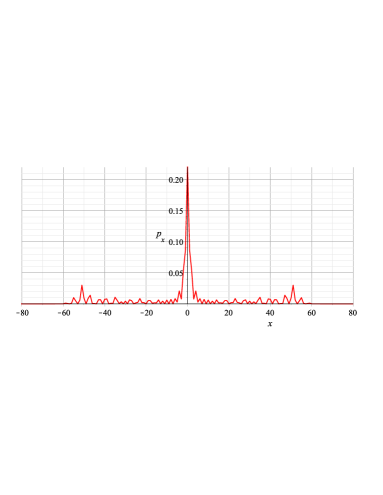
Figure 3: Probability distribution of the coinless 3-state QW after 20 steps with initial state located at $x=0$. The sharp peak at the origin is the signature of the locality always present in the 3-state case.

VI Coinless QW on the Cycle

Consider a cycle with even number $N$ of sites. The associated Hilbert space ${\cal H}^{N}$ is spanned by $\{{\left|{x}\right\rangle},0\leq x\leq N-1\}$. Some of the equations of Sec. V.1 apply here after a formal replacement $\exp(i)\rightarrow\omega_{N}$, where $\omega_{N}=\textrm{e}^{2\pi i/N}$. Eqs. (29) and (30) must be changed so that the dummy index $x$ runs from 0 to $N/2-1$.

The Fourier transform is based on the following set of orthonormal vectors:

$${\left|{\tilde{\psi}_{k}^{\textrm{0}}}\right\rangle} = \sqrt{\frac{2}{N}}\sum_{x=0}^{\frac{N}{2}-1}\omega_{N}^{-2xk}{\left|{2x}\right\rangle},$$ (55)

$${\left|{\tilde{\psi}_{k}^{\textrm{1}}}\right\rangle} = \sqrt{\frac{2}{N}}\sum_{x=0}^{\frac{N}{2}-1}\omega_{N}^{-(2x+1)k}{\left|{2x+1}\right\rangle},$$ (56)

where $0\leq k\leq N/2-1$. Eqs. (32) and (33) must be changed to

$$A = -\cos\alpha\cos\beta+\sin\alpha\sin\beta\,\textrm{e}^{i(\phi_{1}+\phi_{2})}\omega_{N}^{2k},$$ (57)

$$B = \sin\alpha\cos\beta\,\textrm{e}^{i\phi_{1}}\omega_{N}^{k}+\cos\alpha\sin\beta\,\textrm{e}^{-i\phi_{2}}\omega_{N}^{-k},$$ (58)

and Eq. (38) to

$$U=\sum_{k=0}^{\frac{N}{2}-1}\left(\textrm{e}^{i\theta}{\left|{v_{k}^{+}}\right\rangle}{\left\langle{v_{k}^{+}}\right|}+\textrm{e}^{-i\theta}{\left|{v_{k}^{-}}\right\rangle}{\left\langle{v_{k}^{-}}\right|}\right),$$ (59)

Eqs. (40) and (41) to

$$\psi_{2x}(t)=\sqrt{\frac{2}{N}}\sum_{x=0}^{\frac{N}{2}-1}|B|^{2}\omega_{N}^{-2xk}\left(\frac{\textrm{e}^{i\theta t}}{C^{+}}+\frac{\textrm{e}^{-i\theta t}}{C^{-}}\right)$$ (60)

and

$$\psi_{2x+1}(t)=\sqrt{\frac{2}{N}}\sum_{x=0}^{\frac{N}{2}-1}\frac{B\sin\theta t}{\sin\theta}\,\omega_{N}^{-(2x+1)k}.$$ (61)

If 4 divides $N$ and $\alpha=\beta$ and $\phi_{1}=\phi_{2}$, eigenvector (35) and the normalization constants $C^{\pm}$ are zero for $k=N/4$. The eigenvectors for this special value of $k$ must be calculated separately.

VI.1 Mixing Time

Let ${\left|{v_{k}}\right\rangle}$ and $\textrm{e}^{i\lambda_{k}}$ denote the eigenvectors and eigenvalues of ${\cal U}$. Then

$${\cal U}=\sum_{k=0}^{N-1}\textrm{e}^{i\lambda_{k}}{\left|{v_{k}}\right\rangle}{\left\langle{v_{k}}\right|}.$$ (62)

The time-averaged probability density function (PDF) is defined by

$$\overline{p}_{x}(T)=\frac{1}{T}\sum_{t=0}^{T-1}p_{x}(t),$$ (63)

where by Eq. (62), we obtain for the PDF on a finite-length cycle

$$\overline{p}_{x}(T)=\sum_{k,k^{\prime}=0}^{N-1}c_{k}^{*}c_{k^{\prime}}v_{k,x}v_{k^{\prime},x}^{*}\,\frac{1}{T}\sum_{t=0}^{T-1}\textrm{e}^{i(\lambda_{k}-\lambda_{k^{\prime}})T},$$ (64)

setting $c_{k}=\langle 0|v_{k}\rangle$ and $v_{k,x}=\langle x|v_{k}\rangle$ for a walker that departs from the origin. With

$$\frac{1}{T}\sum_{t=0}^{T-1}\textrm{e}^{i(\lambda_{k}-\lambda_{k^{\prime}})T}=\delta_{\lambda_{k},\lambda_{k^{\prime}}}+(1-\delta_{\lambda_{k},\lambda_{k^{\prime}}})\frac{\textrm{e}^{i(\lambda_{k}-\lambda_{k^{\prime}})T}-1}{T(\textrm{e}^{i(\lambda_{k}-\lambda_{k^{\prime}})}-1)}$$ (65)

we obtain

$$\overline{p}_{x}(T)=\pi_{x}+\frac{1}{T}\sum_{\begin{subarray}{c}k,k^{\prime}=0\\ \lambda_{k}\neq\lambda_{k^{\prime}}\end{subarray}}^{N-1}c_{k}^{*}c_{k^{\prime}}v_{k,x}v_{k^{\prime},x}^{*}\,\frac{\textrm{e}^{i(\lambda_{k}-\lambda_{k^{\prime}})T}-1}{\textrm{e}^{i(\lambda_{k}-\lambda_{k^{\prime}})}-1},$$ (66)

with

$$\pi_{x} := \lim_{T\rightarrow\infty}\overline{p}_{x}(T)\,=\sum_{\begin{subarray}{c}k,k^{\prime}=0\\ \lambda_{k}=\lambda_{k^{\prime}}\end{subarray}}^{N-1}c_{k}^{*}c_{k^{\prime}}v_{k,x}v_{k^{\prime},x}^{*}.$$ (67)

The mixing time $\tau_{\epsilon}$ is defined as

$$\tau_{\epsilon}=\min\{T\,|\,\forall t\geq T,\,D(\overline{p}(t),\pi)\leq\epsilon\},$$ (68)

where $D(\overline{p}(t),\pi)$ is the total variation distance (TVD) defined by

$$D(\overline{p}(t),\pi)=\frac{1}{2t}\sum_{x=0}^{N-1}\left|\sum_{\begin{subarray}{c}k,k^{\prime}=0\\ \lambda_{k}\neq\lambda_{k^{\prime}}\end{subarray}}^{N-1}c_{k}^{*}c_{k^{\prime}}v_{k,x}v_{k^{\prime},x}^{*}\,\frac{\textrm{e}^{i(\lambda_{k}-\lambda_{k^{\prime}})t}-1}{\textrm{e}^{i(\lambda_{k}-\lambda_{k^{\prime}})}-1}\right|.$$ (69)

The mixing time captures the notion of the convergence of the time-averaged density to the limiting PDF.

VI.1.1 Time-Averaged Probability Density Function in the Large-Time Limit

In analogy with the discussion leading to the eigenvalues of the propagator on the infinite line in Eq. (37), the coefficients $v_{k,x}$ are given by

$$v_{k,2x} = \frac{-\sqrt{2}B^{*}}{\sqrt{NC^{\pm}}}\,\omega_{N}^{-2xk}$$ (70)

$$v_{k,2x+1} = \frac{\sqrt{2}\,(\textrm{e}^{\pm i\theta}-A)}{\sqrt{NC^{\pm}}}\,\omega_{N}^{-(2x+1)k}$$ (71)

and $c_{k}=v_{k,0}$, where the sign plus must be taken for $0\leq k<N/2$ and the sign minus for $N/2\leq k<N$. Using the fact that $\lambda_{k}=\lambda_{k^{\prime}}$ when $k^{\prime}=k$ and $k^{\prime}=N/2-k$, and Eq. (67), the limiting PDF for even sites is

$$\pi_{2x}=\frac{2}{N^{2}}+\frac{4}{N^{2}}\sum_{k=1}^{\frac{N}{2}-1}|B|^{4}\left(\frac{1}{{C^{+}}^{2}}+\frac{1}{{C^{-}}^{2}}+\frac{2\cos\frac{8\pi k\,x}{N}}{C^{+}C^{-}}\,(1-\delta_{k\frac{N}{4}})\right).$$ (72)

Notice that the last term vanishes when $k=N/4$. For odd sites, the limiting probability is

$$\pi_{2x+1}=\frac{2}{N^{2}}\sum_{k=0}^{\frac{N}{2}-1}\frac{|B|^{2}}{\sin^{2}\theta}+\frac{1}{N^{2}}\sum_{k=1}^{\frac{N}{2}-1}\frac{1-\delta_{k\frac{N}{4}}}{\sin^{2}\theta}\left(B^{2}\omega_{N}^{-2k(2x+1)}+{B^{*}}^{2}\omega_{N}^{2k(2x+1)}\right).$$ (73)

Fig. 4 shows the limiting PDF for even and odd sites separately (the parameters are $N=200$, $\alpha=\pi/2$, $\beta=2\pi/3$, and $\phi_{1}=\phi_{2}=0$). Both PDF are almost constant except for the spikes around $x=0$ and $x=N/2$. If 4 does not divide $N$, there are no spikes at $x=N/2$.

Figure 4: Limiting probability density function for $N=200$. Upper blue (lower red) curve is the PDF for even (odd) sites.

If is interesting to compare those results with the corresponding ones for the coined QW Aharonov et al. (2001); Portugal (2013); Bednarska et al. (2003). In both cases, the limiting PDFs are remarkably similar. If $N$ is even, the limiting PDF for the coined case also have spikes at $x=0$ and $x=N/2$. On the other hand, if $N$ is odd, the limiting PDF for the coined case is constant for all $x$ while there is no simple tessellation in the coinless case that allows the definition of an interesting evolution operator in this case.

VI.1.2 Asymptotic Behavior of the Mixing Time

From Eq. (69), we see that that the TVD between the average and the limiting PDF depends on $t$ in two distinct ways: 1) it decreases linearly with $t$ because the pre-factor $1/t$, 2) it oscillates because the term $\textrm{e}^{i(\lambda_{k}-\lambda_{k^{\prime}})t}$. The oscillatory term makes difficult the exact determination of $\tau_{\epsilon}$ in terms of $\epsilon$ and the system size $N$. We use the Riemann-Lebesgue lemma to argue that this oscillatory term can be disregarded to calculate the asymptotic scaling behavior of the mixing time.

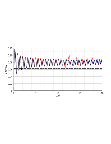
Figure 5: Rescaled total variation distance ($t\,\textrm{TVD}/N$) as function of $t/N$ for $N=500,2000,5000$ with colors red, blue, and black, respectively. The dashed line corresponds to the TVD without the oscillatory term, i.e. after removing the term $\exp(i(\lambda_{k}-\lambda_{k^{\prime}})t)$.

Fig. 5 shows the rescaled graphs of $tD(\overline{p}(t),\pi)/N$ as a function of $t/N$ for three different values of $N$ (the parameters are $\alpha=\pi/2$, $\beta=2\pi/3$, and $\phi_{1}=\phi_{2}=0$). The curves are strikingly coincident for small $t/N$ and gradationally becomes more distinguishable as $t/N$ increases because the curves have different amplitudes while still keeping similar wavelengths. The same coincidence happens for larger values of $N$ that we can verify numerically. This numerical result implies that, for large $N$, $D(\overline{p}(t),\pi)$ has the form $\frac{N}{t}f\big{(}\frac{t}{N}\big{)}$, where $f\big{(}\frac{t}{N}\big{)}$ is an oscillatory function the amplitude of which does not depend on $N$. We argue based on the Riemann-Lebesgue lemma that the amplitude of the oscillation dies off when $t/N$ gets larger.

From Eq. (69) we obtain the following bound for the TVD

$$D(\overline{p}(t),\pi)\leq\frac{1}{2t}\sum_{x=0}^{N-1}\left(\left|\sum_{k,k^{\prime}}f_{k,k^{\prime},x}\right|+\left|\sum_{k,k^{\prime}}f_{k,k^{\prime},x}\textrm{e}^{i\Delta_{k,k^{\prime}}t}\right|\right),$$ (74)

where the sums over $k,k^{\prime}$ are the same as before (i.e., such that $\lambda_{k}\not=\lambda_{k^{\prime}}$), $\Delta_{k,k^{\prime}}=\lambda_{k}-\lambda_{k^{\prime}}$ and

$$f_{k,k^{\prime},x}\,=\,\frac{c_{k}^{*}c_{k^{\prime}}v_{k,x}v_{k^{\prime},x}^{*}}{\textrm{e}^{i(\lambda_{k}-\lambda_{k^{\prime}})}-1}.$$ (75)

For large $N$, the second term of Eq. (74) can be approximated by a double integral and the Riemann-Lebesgue lemma states that it goes to zero when $t\rightarrow\infty$. (There may be a small neighborhood in the integration domain where $\Delta_{k,k^{\prime}}\sim 1/N$ such that the lemma would not apply, however, the weight of this contribution is negligible.) This proves that $\tau_{\epsilon}$ is $\Theta(1/\epsilon)$ for any fixed $N$.

By analysing the sign of $f_{k,k^{\prime},x}$, we can simplify the first term of (74), which is given by

$$\sum_{x=0}^{N-1}\left|\sum_{k,k^{\prime}}f_{k,k^{\prime},x}\right| = \frac{4}{N^{2}}\sum_{\begin{subarray}{c}k,k^{\prime}=0\\ k\neq k^{\prime}\\ k+k^{\prime}\neq\frac{N}{2}\end{subarray}}^{\frac{N}{2}-1}\frac{\left|B_{k}B_{k^{\prime}}\right|^{2}}{C_{k}^{+}C_{k^{\prime}}^{+}}\,(1-g^{-}_{k,k^{\prime}})+$$ (76)

$$\frac{4}{N^{2}}\sum_{k,k^{\prime}}^{\frac{N}{2}-1}\frac{\left|B_{k}B_{k^{\prime}}\right|^{2}}{C_{k}^{+}C_{k^{\prime}}^{-}}\,(1+(\delta_{k,k^{\prime}}-1)\,g^{+}_{k,k^{\prime}})+$$

$$\frac{2}{N}\sum_{k}^{\frac{N}{2}-1}\frac{\left|B_{k}\right|^{2}}{{C_{k}^{+}}{C_{k}^{-}}}{(\textrm{e}^{i\theta_{k}}-A_{k})(\textrm{e}^{-i\theta_{k}}-A_{k})},$$

where

$$g^{\pm}_{k,k^{\prime}}\,=\,\frac{(-1)^{k-k^{\prime}}-\cos\frac{2\pi(k-k^{\prime})}{N}}{\sin\frac{2\pi(k-k^{\prime})}{N}}\,\frac{1+\cos(\theta_{k}\pm\theta_{k^{\prime}})}{\sin(\theta_{k}\pm\theta_{k^{\prime}})}.$$ (77)

Fig. 6 shows the plot of the first (red $+$) and second (blue $\times$) terms of the rhs of Eq. (76) as a function of $N$. The third term has no poles and can be calculated numerically by converting the sum into an integral, which is independent of $N$ for large $N$. This result, together with Fig. 5, numerically shows that the TVD is $\Theta(N)$. Then $\tau_{\epsilon}=\Theta(N/\epsilon)$, that is, $\tau_{\epsilon}$ is propotional to $N/\epsilon$ for $N$ large enough and $\epsilon$ small enough. Notice that the corresponding result for the coined QW on cycles (with odd $N$) is the bound $O(N\log N/\epsilon^{3})$ found in Ref. Aharonov et al. (2001).

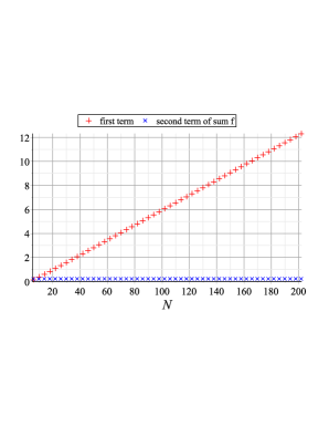
Figure 6: Behavior of the first (red $+$) and second (blue $\times$) terms of Eq. (76) as a function of $N$. The first term clearly is $O(N)$.

VII Conclusions

In conclusion, we have shown a formal connection between the coinless and coined one-dimensional QW, obtained a number of asymptotic properties for coinless QWs on infinite 1D-lattice, showed Anderson-like localization in coinless 3-state models, and analyzed the asymptotic behavior of the mixing times on cycles. The numerical results suggest that $\tau_{\epsilon}=\Theta(N/\epsilon)$.

A comparison between the coinless and the coined QWs reveals striking similarities. For instance, the two-step propagator combined with a initial conditions localized inside the cell that contains the origin produce asymptotic behavior similar to coined QWs departing from the origin with generic initial coin state. And just as for the coined QW, where the $2x2$ Grover coin degenerates in $D=1$ to make a non-trivial symmetric QW at optimal speed $c$ impossible, we find here that the $D=1$ tessellation in Eqs. (6) and (7) has only trivial solutions for $v_{0}\to 1$ while in $D=2$ and the 3-state model it provides both symmetry and optimal speed. Finally, we note that using square-block tessellations of size $2^{D}$ in $D$ dimensions becomes impractical for $D>2$, as the rank of the reduced space grows exponentially as $2^{D}$ while the degree of each site only grows $\sim 2D$. That suggests that better tessellations would need to be found, such as a $D$-dimensional version of “3-crosses”, as a generalization of the 3-patches in Fig. 1.

The nature of coinless QWs depend on the choice of the tessellation. We have used simple 2-blocks neighboring sites which cover the entire lattice. Many other tessellations are possible, as we have demonstrated for the 3-site tessellation for one-dimensional QW as showed in Fig. 1, for example. Note that in this case neither of the two-stroke tessellation individually covers the entire lattice, only the combination of both tessellations. We believe that a symmetric and overlapping tessellation with a combined coverage is sufficient for an optimal coinless quantum search. It will be interesting to analyze in more detail which kind of physical behavior the choice of a tessellation can provide, such as for displacement, localization (Inui et al., 2005; Falkner and Boettcher, 2014), and mixing. This physical analysis helps to understand algorithmic applications of this QW model, such as searching for a marked vertex.

References

- Aharonov et al. (1993) Y. Aharonov, L. Davidovich, and N. Zagury, Phys. Rev. A 48, 1687 (1993).
- Aharonov et al. (2001) D. Aharonov, A. Ambainis, J. Kempe, and U. Vazirani, in Proc. 33th STOC (ACM, New York, NY, 2001), pp. 50–59.
- Aldous and Fill (200X) D. J. Aldous and J. A. Fill, Reversible Markov Chains and Random Walks on Graphs (Book in preparation, http://www.stat.berkeley.edu/~aldous/book.html, 200X).
- Shenvi et al. (2003) N. Shenvi, J. Kempe, and K. Whaley, Phys. Rev. A 67, 052307 (2003).
- Ambainis et al. (2005) A. Ambainis, J. Kempe, and A. Rivosh, in Proc. 16th SODA (2005), pp. 1099–1108.
- Portugal (2013) R. Portugal, Quantum Walks and Search Algorithms (Springer, Berlin, 2013).
- Patel et al. (2005) A. Patel, K. S. Raghunathan, and P. Rungta, Phys. Rev. A 71, 032347 (2005).
- Meyer (1996) D. Meyer, Journal of Statistical Physics 85, 551 (1996), ISSN 0022-4715, URL http://dx.doi.org/10.1007/BF02199356.
- Patel and Raghunathan (2012) A. Patel and K. S. Raghunathan, Phys. Rev. A 86, 012332 (2012).
- Falk (2013) M. Falk, arXiv:1303.4127 (2013).
- Ambainis et al. (2013) A. Ambainis, R. Portugal, and N. Nahimov, arXiv:1312.0172 (2013).
- Childs and Ge (2014) A. M. Childs and Y. Ge, Phys. Rev. A 89, 052337 (2014).
- Farhi and Gutmann (1998) E. Farhi and S. Gutmann, Phys. Rev. A 58, 915 (1998).
- Szegedy (2004) M. Szegedy, Proceedings 45th IEEE Symposium on the Foundations of Computer Science pp. 32–41 (2004).
- Ambainis et al. (2001) A. Ambainis, E. Bach, A. Nayak, A. Vishwanath, and J. Watrous, Annual ACM Symposium on Theory of Computing 33, 37 (2001).
- Bach et al. (2004) E. Bach, S. Coppersmith, M. P. Goldschen, R. Joynt, and J. Watrous, Journal of Computer and System Sciences 69, 562 (2004).
- Inui and Konno (2005) N. Inui and N. Konno, Physica A 353, 333 (2005).
- Falkner and Boettcher (2014) S. Falkner and S. Boettcher, Phys. Rev. A 90, 012307 (2014).
- Itzykson and Drouffe (1989) C. Itzykson and J.-M. Drouffe, Statistical Field Theory (Cambridge University Press, 1989).
- Redner (2001) S. Redner, A Guide to First-Passage Processes (Cambridge University Press, Cambridge, 2001).
- Weiss (1994) G. H. Weiss, Aspects and Applications of the Random Walk (North-Holland, Amsterdam, 1994).
- Venegas-Andraca (2012) E. Venegas-Andraca, Quantum Information Processing 11, 1015 (2012).
- Bender and Orszag (1978) C. M. Bender and S. A. Orszag, Advanced Mathematical Methods for Scientists and Engineers (McGraw-Hill, New York, 1978).
- Bednarska et al. (2003) M. Bednarska, A. Grudka, P. Kurzynski, T. Luczak, and A. Wójcik, Physics Letters A 317, 21 (2003).
- Inui et al. (2005) N. Inui, N. Konno, and E. Segawa, Phys. Rev. E 72, 056112 (2005).