Sparsifying Preconditioner for the Lippmann-Schwinger Equation

Abstract.

The Lippmann-Schwinger equation is an integral equation formulation for acoustic and electromagnetic scattering from an inhomogeneous media and quantum scattering from a localized potential. We present the sparsifying preconditioner for accelerating the iterative solution of the Lippmann-Schwinger equation. This new preconditioner transforms the discretized Lippmann-Schwinger equation into sparse form and leverages the efficient sparse linear algebra algorithms for computing an approximate inverse. This preconditioner is efficient and easy to implement. When combined with standard iterative methods, it results in almost frequency-independent iteration counts. We provide 2D and 3D numerical results to demonstrate the effectiveness of this new preconditioner.

1. Introduction

This paper is concerned with the efficient solution of the Lippmann-Schwinger equation, which describes time-harmonic scattering from inhomogeneous media in acoustics and electromagnetics as well as time-harmonic scattering from localized potentials in quantum mechanics. The simplest form of this equation comes from inhomogeneous acoustic scattering. Let $\omega$ be the frequency of the time-harmonic wave and denote the index of refraction by $1-m(x)$. The inhomogeneity $m(x)$ is a function supported in a compact domain $\Omega\subset\mathrm{R}^{d}$ of size $O(1)$, so the index of refraction is $1$ outside $\Omega$. Given an incoming wave $u_{I}(x)$ that satisfies the free space Helmholtz equation

$$(\Delta+\omega^{2})u_{I}(x)=0,\quad x\in\mathrm{R}^{d}$$

the problem of scattering from inhomogeneous media is to find the scattered field $u(x)$ such that the total field $u(x)+u_{I}(x)$ satisfies

(1) $$(\Delta+\omega^{2}(1-m(x)))(u(x)+u_{I}(x))=0,\quad x\in\mathrm{R}^{d}$$

and $u(x)$ obeys the Sommerfeld radiation condition:

(2) $$\lim_{r\rightarrow\infty}r^{(d-1)/2}\left(\frac{\partial u}{\partial r}-i\omega u\right)=0.$$

For the free space Helmholtz operator $-(\Delta+\omega^{2})$, the Green’s function is given by

$$G(x)=\begin{cases}\frac{1}{2i\omega}\exp(i\omega|x|),&d=1,\\ \frac{i}{4}H^{1}_{0}(\omega|x|),&d=2,\\ \frac{1}{4\pi|x|}\exp(i\omega|x|),&d=3.\end{cases}$$

Rewriting (1) as

$$(-\Delta-\omega^{2}+\omega^{2}m(x))u(x)=-\omega^{2}m(x)u_{I}(x),\quad x\in\mathrm{R}^{d}$$

and convolving it with $G(x)$ gives

(3) $$u+G\ast(\omega^{2}mu)=G\ast(-\omega^{2}mu_{I}),$$

which is the Lippmann-Schwinger equation written in terms of the scattered field $u(x)$. One can also write the Lippmann-Schwinger in terms of the total field $u(x)+u_{I}(x)$, but we shall stick to (3) since its unknown $u(x)$ satisfies the Sommerfeld radiation condition. For the inhomogeneous electromagnetic scattering and quantum scattering, the same derivation results in integral equations similar to (3).

For high frequency wave fields (i.e., $\omega$ large), computing numerical solution of scattering in inhomogeneous media remains a challenging computational problem especially in 3D. For practical and numerical purposes, working with (3) rather than (1) offers several advantages.

• First, (3) is written in terms of $u(x)$ only for $x\in\Omega$ as $m(x)=0$ for $x\not\in\Omega$. Therefore, the unknown function in (3) is defined on the compact set $\Omega$ versus the whole space $\mathrm{R}^{d}$ as in (1).

• Second, once $u(y)$ for $y\in\Omega$ is computed, the whole scattered field in $\mathrm{R}^{d}$ defined via

  $$u(x)=-\int_{\Omega}G(x-y)\omega^{2}m(y)(u(y)+u_{I}(y))dy,\quad\forall x\in\mathrm{R}^{d}$$

  satisfies the Sommerfeld radiation condition (2) automatically. However, for (1) a special treatment such as perfectly matched layer (PML) [berenger-1994, chew-1994] or absorbing boundary condition (ABC) [engquist-77] is required to approximate (2) at a finite distance.

• Third, the convolution structure of (3) allows for rapid application of the integral operator via the fast Fourier transform (FFT) [cooley-1965].

• Finally, most treatments of (1) for high-frequency problems suffer from the pollution effect [babuska-1997], due to the error from the local finite difference or finite element stencils. This problem does not show up in (3) because of the explicit introduction of the Green’s function.

However, working with (3) also brings a couple of numerical issues. Discretizing the integral equation (3) results a dense linear system, which renders typical direct solvers impractical except for 1D problems. For this reason, most numerical solutions of the Lippmann-Schwinger equation use iterative solvers. Since the Lippmann-Schwinger equation is numerically ill-conditioned, standard iterative methods without preconditioning requires a huge number of iterations for high frequency problems. This is especially true when the inhomogeneity $m(x)$ has sharp transitions (see [duan-2009] for example). Therefore, there is a clear need for developing good preconditioners for the Lippmann-Schwinger equation.

There has been a substantial amount of work on computing numerical solutions of the Lippmann-Schwinger in the recent literature, for example [andersson-2005, bruno-2004, chen-2002, lanzara-2004, sifuentes-2010, vainikko-2000]. Several of these methods are concerned with the design of efficient preconditioners. In [bruno-2004], Bruno and Hyde constructed a preconditioner by replacing the inhomogeneity $m(x)$ with a piecewise constant and radially symmetric approximation and then inverting the associated approximate integral operator with semi-analytic methods. Such a preconditioner is effective when there exists a good piecewise constant and radially symmetric approximation, and naturally deteriorates when there is no such approximation.

In [chen-2002], Chen proposed a method for solving the 2D Lippmann-Schwinger equation using a technique that is now often referred as recursive interpolative decomposition or recursive skeletonization. This method generates in $O(N^{3/2})$ steps an approximate inverse which can be used either as a direct solver if the accuracy is sufficient or as a preconditioner. More advanced and efficient methods for general integral equations have been proposed in [corona-2014] for 2D problems and in [ho-2013] for both 2D and 3D problems. These recent methods achieve quasi-linear complexity for integral equations with non-oscillatory kernels, but fall back to the same $O(N^{3/2})$ cost for 2D high frequency Lippmann-Schwinger equations. For all these methods, the prefactor of the complexity depends on the required accuracy and can be very large when they are used as direct solvers.

There have also been attempts to apply two-grid and multigrid methods to precondition the Lippmann-Schwinger equation (see [sifuentes-2010] for example). However, due to the highly oscillatory nature of the solution field, such methods tend to improve the iteration number at most by a constant factor.

In this paper, we introduce a new preconditioner called the sparsifying preconditioner for the Lippmann-Schwinger equation. The main idea is to transform the discretized Lippmann-Schwinger equation approximately into a sparse linear system. This is possible since the scattered field indeed satisfies the Helmholtz equation in $\Omega$ and approximately the absorbing-type boundary conditions on $\partial\Omega$. Once the sparse linear system is ready, we invert it by leveraging the efficiency of sparse linear algebra algorithms.

The rest of this paper is organized as follows. In Section 2 we introduce the discretization scheme and describe the main idea. Sections 3 and 4 explain the details of the sparsifying preconditioner for rectangular domains and general domains, respectively. Section 5 extends our approach to the Laplace equation with potential perturbation. Finally, discussions and future work are given in Section 6.

2. Discretization and main idea

The sparsifying preconditioner to be presented is mostly independent of the discretization scheme and the dimension. We assume that a Nyström method is used in order to keep the presentation simple. Our discussion focuses on the 2D and 3D cases, since the 1D problem is not computationally challenging.

At any point $x\in\Omega$, the local wave velocity is given by $c(x)=(1-m(x))^{-1/2}$. At frequency $\omega$, the local wavelength at $x$ is equal to $\lambda(x)=(2\pi/\omega)(1-m(x))^{-1/2}$.

2.1. Discretization

Let us first consider the 2D case. The domain $\Omega$ is discretized with a uniform grid of step size $h$, where $h$ is chosen such that there are at least a few grid points per wavelength across the domain. Such a uniform grid is convenient when the variation in $c(x)$ is not too large. For problems with large variations in $c(x)$, an adaptively-refined grid should be used instead. The grid points are indexed by integer pairs $i=(i_{1},i_{2})$ with location given by $x_{i}=ih=(i_{1}h,i_{2}h)$.

We assume that $m(x)$ is zero within two layers of grid points from the boundary $\partial\Omega$, which can be easily satisfied by slightly enlarging $\Omega$ if necessary. The discretization uses $m_{i}=m(x_{i})$ and let $u_{i}$ be the numerical approximation to $u(x_{i})$. Writing the integral on the left hand side of (3) explicitly at the point $x_{i}$ gives

(4) $$(G\ast(\omega^{2}mu))(x_{i})=\int_{\Omega}G(x_{i}-y)(\omega^{2}m(y)u(y))dy$$

and this integral is approximated with numerical quadrature using the grid points in $\Omega$.

When $m(x)$ is discontinuous, discretizing (4) efficiently and accurately is a non-trivial task and we refer to [beylkin-2008, beylkin-2009] for recent developments. For simplicity, we assume here that $m(x)$ is smooth (but still with possible sharp transitions) and that the grid size $h$ is chosen to sufficiently resolve the transitions in $m(x)$. For such $m(x)$, the discretization of (4) is more straightforward and the only difficulty is the singularity of $G(x)$ at the origin. A simple quadrature rule is

$$\int_{\Omega}G(x_{i}-y)(\omega^{2}m(y)u(y))dy\approx\sum_{j:x_{j}\in\Omega}k_{i-j}\omega^{2}m_{j}u_{j},$$

where

$$k_{t}=G(ht)h^{2},\quad t\not=(0,0)$$

and $k_{(0,0)}$ is given by a quadrature correction near the origin. This is a one-point correction of the trapezoidal rule and gives an accuracy of O($h^{4}\log(1/h))$ (see [duan-2009] for example). There are also higher order versions that correct the grid points in the neighborhood of the origin and they do not affect the following discussion of the sparsifying preconditioner significantly.

After quadrature approximation, the discrete form of the Lippmann-Schwinger equation (3) takes the form, for $i$ with $x_{i}\in\Omega$,

(5) $$u_{i}+\sum_{j:x_{j}\in\Omega}k_{i-j}\omega^{2}m_{j}u_{j}=g_{i},$$

where $g_{i}$ is the discretized value of the right hand side of (3). In a slight abuse of notation, we define $u$ to be the vector with entries given by $u_{i}$ and similarly for $g$ and $m$. Then, (5) can be written as

(6) $$(I+K\omega^{2}m)u=g,$$

where $K$ is the matrix with entries defined via $K(i,j)=k_{i-j}$ and $m$ is understood as operator of multiplying with the vector $m$ entry-wise.

The situation for the 3D case is almost the same except that $i$ is now an integer triple $(i_{1},i_{2},i_{3})$ and $k_{t}=G(th)h^{3}$ for $t\not=(0,0,0)$.

2.2. Main idea

The main idea of our approach is to find a sparse and local operator $Q$ such that in

$$Q(I+K\omega^{2}m)u=Qg$$

the operator $Q(I+K\omega^{2}m)$ is also numerically sparse and localized. This is possible since the scattered field $u$ satisfies

• the Helmholtz equation (1) in the interior of $\Omega$, and

• approximately the absorbing-type boundary conditions on the boundary of $\Omega$.

For a grid point indexed by $i$, we define its neighborhood $\mu(i)$ to be

$$\mu(i)=\{j:\|i-j\|_{\infty}\leq 1,x_{j}\in\Omega\}.$$

A grid point $i$ is called an interior point if all the grid points in $\mu(i)$ are also in $\Omega$, and otherwise a boundary point. The set $\mu(i)$ contains 9 points in 2D and 27 points in 3D for an interior point, but has fewer points for a boundary point. Let $N_{I}$ and $N_{B}$ denote the numbers of interior and boundary grid points, respectively. The total number of grid points $N$ is equal to $N_{I}+N_{B}$.

For the interior points, we shall design a matrix $A$ of size $N_{I}\times N$, with the rows indexed by the interior grid points. For a fixed interior index $i$, the row $A(i,:)$ satisfies two conditions:

• $A(i,:)$ has support in $\mu(i)$, and

• $A(i,:)K(:,j)\equiv A(i,\mu(i))K(\mu(i),j)\approx 0$ for any $j\not\in\mu(i)$, or, equivalently $A(i,:)K(:,\mu(i)^{c})\approx 0$.

Once $A$ has been calculated, we can define a sparse matrix $C$ of the same size such that

• $C(i,:)$ has support in $\mu(i)$, and

• $C(i,\mu(i)):=A(i,\mu(i))K(\mu(i),\mu(i))$.

The above conditions imply that

• $C$ and $A$ are sparse operators that represent a local stencil, and

• $AK\approx C$.

Therefore,

(7) $$A(I+K\omega^{2}m)\approx(A+C\omega^{2}m).$$

For the boundary points, we shall design a matrix $B$ of size $N_{B}\times N$, with the rows indexed by the boundary grid points. For a fixed boundary index $i$, the row $B(i,:)$ satisfies two conditions:

• $B(i,:)$ has support in $\mu(i)$, and

• $B(i,:)K(:,j)\equiv B(i,\mu(i))K(\mu(i),j)\approx 0$ for any $j\not\in\mu(i)$.

Since $m_{j}=0$ for any grid point $j$ within two layers from the boundary and $i$ is a boundary point, $m_{j}=0$ for $j\in\mu(i)$. Therefore, the second condition implies that

$$B(i,:)(K\omega^{2}m)(:,:)\approx 0.$$

Hence,

(8) $$B(I+K\omega^{2}m)\approx B.$$

Applying matrices $A$ and $B$ to both sides of (6) yields

(9) $$\begin{bmatrix}A\\ B\end{bmatrix}(I+K\omega^{2}m)u=\begin{bmatrix}A\\ B\end{bmatrix}g.$$

Combining (7) and (8) with (9) gives

(10) $$\begin{bmatrix}A+C\omega^{2}m\\ B\end{bmatrix}u\approx\begin{bmatrix}A\\ B\end{bmatrix}g.$$

This suggests defining the preconditioner as the mapping from $g$ to $u$ given by

(11) $$u\Leftarrow\begin{bmatrix}A+C\omega^{2}m\\ B\end{bmatrix}^{-1}\begin{bmatrix}A\\ B\end{bmatrix}g.$$

Since $A$ and $B$ are sparse, applying these operators on the right hand side is fast. In addition, since $A$, $B$, and $C$ are all designed to be local operators, the linear system solve in (11) can be done efficiently with, for example, the nested dissection method and the multifrontal method [duff-1983, george-1973].

In the following sections, we shall apply this procedure to several different setting. In each case, we explicitly give the construction for $A$ and $B$, analyze the complexity of constructing and applying the preconditioner, and provide numerical results.

3. Rectangular domains

This section considers the case of rectangular $\Omega$.

3.1. Algorithm

Let us consider the 2D case first. For simplicity, let $\Omega=(0,1)^{2}$ and define $n=1/h$ to be the number of points in each dimension. Clearly, $N=n^{2}$, $N_{B}=O(n)$, and $N_{I}=O(n^{2})$. In order for the operator $B$ to serve as a sufficiently accurate approximation to the Sommerfeld radiation condition, we assume that $m(x)$ vanishes in a buffer region of a constant, but small, width near the boundary and the constant $b$ denotes the ratio between the width and the step size.

For each interior point $i$, recall that we require

$$A(i,\mu(i))K(\mu(i),j)\approx 0,\quad\forall j\not\in\mu(i).$$

Since $K$ is translational invariant, it is convenient to require $A$ be so as well. By translating the point $i$ to the origin, it is sufficient to consider the problem of finding a vector $\alpha$ such that

$$\alpha\cdot K(\mu(0),j)\approx 0,\quad\forall j\in I_{n}:=\{j:-n<j_{1},j_{2}<n,j\not\in\mu(0)\}.$$

To solve for $\alpha$, we formulate the following optimization problem

(12) $$\min_{\alpha:\|\alpha\|=1}\|\alpha\cdot K(\mu(0),I_{n})\|^{2}.$$

Through the singular value decomposition $K(\mu(0),I_{n})=USV^{*}$, the solution is given by

$$\alpha=U(:,|\mu(0)|)^{*}$$

and we set $A(i,\mu(i))=\alpha$ for all interior $i$.

For the boundary, there are two separate cases: edge points and corner points. For a boundary point $i$ on an edge (suppose the right one), we require

$$B(i,\mu(i))K(\mu(i),j)\approx 0,\quad\forall j\not\in\mu(i).$$

Translating the point $i$ to the origin gives the sufficient problem of finding $\alpha$ such that

$$\alpha\cdot K(\mu_{E}(0),j)\approx 0,\quad\forall j\in E_{n}:=\{j:-n<j_{1}<-b,-n<j_{2}<n\},$$

where $\mu_{E}(0)$ is the translated copy of $\mu(i)$. To solve for $\alpha$, we consider

(13) $$\min_{\alpha:\|\alpha\|=1}\|\alpha\cdot K(\mu_{E}(0),E_{n})\|^{2}.$$

Once again, the singular value decomposition $K(\mu_{E}(0),E_{n})=USV^{*}$ gives the solution

$$\alpha=U(:,|\mu_{E}(0)|)^{*}$$

and we set $B(i,\mu(i))=\alpha$ for all boundary $i$ on the edges.

For a boundary point $i$ at a corner (suppose the top-right one), we require

$$B(i,\mu(i))K(\mu(i),j)\approx 0,\quad\forall j\not\in\mu(i).$$

Translating the point $i$ to the origin gives the problem of finding $\alpha$ such that

$$\alpha\cdot K(\mu_{C}(0),j)\approx 0,\quad\forall j\in C_{n}:=\{j:-n<j_{1},j_{2}<-b\},$$

where $\mu_{C}(0)$ is the translated copy of $\mu(i)$. To solve for $\alpha$, we consider

(14) $$\min_{\alpha:\|\alpha\|=1}\|\alpha\cdot K(\mu_{C}(0),C_{n})\|^{2}.$$

The singular value decomposition $K(\mu_{C}(0),C_{n})=USV^{*}$ gives the solution

$$\alpha=U(:,|\mu_{C}(0)|)^{*}$$

and we set $B(i,\mu(i))=\alpha$ for all corner points $i$.

Once $A$ and $B$ are known, we compute $C$ and form

(15) $$\begin{bmatrix}A+C\omega^{2}m\\ B\end{bmatrix},$$

which is built from local compact stencils on a uniform rectangular grid. As we mentioned earlier, the nested dissection algorithm is used to compute an factorization of this operator.

The extension to 3D is quite straightforward, except there are three types for boundary points: face points, edge points, corner points. For the translated optimization problem, the point sets are defined via

• interior point

  $$I_{n}:=\{j:-n<j_{1},j_{2},j_{3}<n,j\not\in\mu(0)\},$$

• surface point (suppose on $x_{1}=1$)

  $$F_{n}:=\{j:-n<j_{1}<-b,-n<j_{2},j_{3}<n\},$$

• edge point (suppose on $x_{1}=1,x_{2}=1$)

  $$E_{n}:=\{j:-n<j_{1},j_{2}<-b,-n<j_{3}<n\},$$

• corner point (suppose at $x_{1}=2,x_{2}=1,x_{3}=1$)

  $$C_{n}:=\{j:-n<j_{1},j_{2},j_{3}<-b\}.$$

3.2. Complexity

Here we analyze the cost of constructing and applying the sparsifying preconditioner.

In 2D, the setup algorithm consists of two parts: computing the singular value decompositions and factorizing (15) with the nested dissection algorithm. The former has a $O(n^{2})=O(N)$ cost while the latter takes $O(n^{3})=O(N^{3/2})$ steps. Therefore, the total setup cost is $O(N^{3/2})$. Applying the preconditioner is essentially a solve with the nested dissection algorithm, which has $O(n^{2}\log n)=O(N\log N)$ complexity.

In 3D, factorizing (15) with the nested dissection algorithm has an $O(n^{6})=O(N^{2})$ cost and this dominates the setup cost. The cost of applying the preconditioner is equal to $O(n^{4})=O(N^{4/3})$, which is the cost of a nested dissection solve.

3.3. Numerical results

This preconditioner and the necessary nested dissection algorithm are implemented in Matlab. The numerical results below are obtained on a desktop computer with CPU speed at 2.0Hz. For the iterative solver the GMRES algorithm is used with relative tolerance equal to $10^{-6}$. The inhomogeneity $m(x)$ is confined in the unit cube and the velocity field $c(x)$ for each example is between $2/3$ and $1$. The grid step size $h$ is chosen such that there are $6$ points per wavelength for the homogeneous region. This ensures a minimum of 4 points per wavelength across the whole domain.

The 2D case is tested with two examples: a Gaussian bump and a smoothed square cavity. The incoming wave is a plane wave pointing downward at frequency $\omega$ and the results are summarized in Figures 1 and 2. The columns of the tables are:

• $\omega$ is the frequency,

• $N$ is the number of unknowns,

• $T_{s}$ is the setup time of the preconditioner in seconds,

• $T_{a}$ is the application time of the preconditioner in seconds,

• $n_{p}$ is the iteration number of the preconditioned iteration, and

• $T_{p}$ is the solution time of the preconditioned iteration in seconds.

The 3D case is also tested with two examples: a Gaussian bump and a smoothed cubic cavity. The incoming wave is again a plane wave pointing downward at frequency $\omega$ and the results are given in Figures 3 and 4.

The results show that the setup and application costs of the preconditioner scale with $\omega$ and $N$ according to the complexity analysis given above. The preconditioner reduces the iteration number dramatically and in fact it becomes essentially frequency-independent.

$\omega$	$N$	$T_{s}$(sec)	$T_{a}$(sec)	$n_{p}$	$T_{p}$(sec)
1.0e+02	9.0e+03	1.3e+00	6.6e-02	5	4.2e-01
2.0e+02	3.6e+04	6.4e+00	2.6e-01	5	1.4e+00
4.0e+02	1.5e+05	3.9e+01	1.0e+00	6	7.8e+00

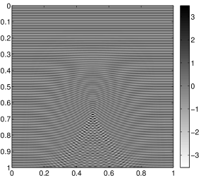
Figure 1. Example 1 of 2D rectangular case. Top: numerical results. Bottom: $c(x)$ (left) and $u(x)+u_{I}(x)$ (right) for the largest $\omega$ value.

$\omega$	$N$	$T_{s}$(sec)	$T_{a}$(sec)	$n_{p}$	$T_{p}$(sec)
1.0e+02	9.0e+03	1.3e+00	7.7e-02	6	4.3e-01
2.0e+02	3.6e+04	7.0e+00	4.1e-01	8	4.1e+00
4.0e+02	1.5e+05	4.2e+01	1.3e+00	8	1.3e+01

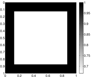
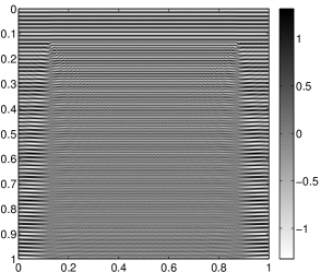
Figure 2. Example 2 of 2D rectangular case. Top: numerical results. Bottom: $c(x)$ (left) and $u(x)+u_{I}(x)$ (right) for the largest $\omega$ value.

$\omega$	$N$	$T_{s}$(sec)	$T_{a}$(sec)	$n_{p}$	$T_{p}$(sec)
2.5e+01	1.2e+04	5.2e+00	6.3e-02	4	2.8e-01
5.0e+01	1.0e+05	1.0e+02	6.4e-01	4	2.9e+00
1.0e+02	8.6e+05	3.2e+03	7.8e+00	4	3.4e+01

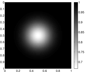
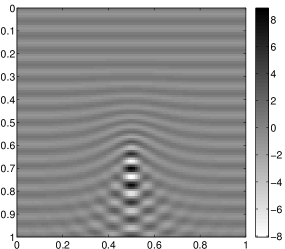
Figure 3. Example 1 of 3D rectangular case. Top: numerical results. Bottom: cross-sections of $c(x)$ (left) and $u(x)+u_{I}(x)$ (right) in the middle of the domain for the largest $\omega$ value.

$\omega$	$N$	$T_{s}$(sec)	$T_{a}$(sec)	$n_{p}$	$T_{p}$(sec)
2.5e+01	1.2e+04	5.6e+00	7.3e-02	6	4.7e-01
5.0e+01	1.0e+05	1.0e+02	5.9e-01	8	5.7e+00
1.0e+02	8.6e+05	2.9e+03	7.7e+00	9	7.5e+01

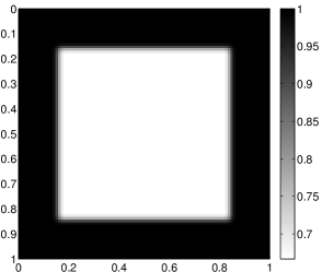
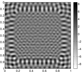
i

Figure 4. Example 2 of 3D rectangular case. Top: numerical results. Bottom: cross-sections of $c(x)$ (left) and $u(x)+u_{I}(x)$ (right) in the middle of the domain for the largest $\omega$ value.

4. General domains

For most problems, the support $\Omega$ of $m(x)$ is not necessarily rectangular. We can apply the approach in Section 3 by embedding $\Omega$ into a rectangular domain. However, this approach increases the number of unknowns significantly, especially in 3D. This section proposes a different approach that does not suffer from this.

4.1. Algorithm

The construction of the operator $A$ for the interior grid points is exactly the same as the one in Section 3. The main difference is in the construction of $B$. For a boundary point $i$, we require

$$B(i,\mu(i))(K\omega^{2}m)(\mu(i),:)\approx 0.$$

Since the local geometry at $i$ can be quite different from point to point, it is impossible to find a uniform stencil $B(i,\mu(i))$ as was done in Section 3. Therefore, one needs to consider $i$ point by point. However, applying the approach of Section 3 to each $i$ individually is too costly since each singular value decomposition costs $O(N)$ steps. To keep the complexity under control, we propose the following randomized approach.

Let $R$ be a Gaussian random matrix of size $N\times r$ where $r=O(1)$ is a constant multiple of the maximum stencil size (i.e., $9$ in 2D and $27$ in 3D) and define the $N\times r$ matrix $T$ via

$$T=(K\omega^{2}m)R.$$

For each boundary $i$, we look for $B(i,\mu(i))$ such that

$$B(i,\mu(i))T(\mu(i),:)\approx 0.$$

This is done by solving the optimization problem

$$\min_{\alpha:\|\alpha\|=1}\|\alpha\cdot T(\mu(i),:)\|^{2}.$$

With the singular value decomposition $T(\mu(i),:)=USV^{*}$, the optimal $\alpha$ is given by

$$\alpha=U(:,|\mu(i)|)^{*}.$$

Finally, we set $B(i,\mu(i))=\alpha$. This process is repeated for each boundary point $i$. Since $T(\mu(i),:)$ is of size $O(1)\times O(1)$, the computational cost of the singular value decomposition setup for each $i$ is also of order $O(1)$.

The effectiveness of this preconditioner depends on the assumption that there exists a good local stencil in $\mu(i)$ for a boundary point $i$. When the domain is convex or nearly convex, such a stencil is guaranteed due to the absorbing-type boundary conditions. However, when the domain is highly non-convex the preconditioner is less effective.

4.2. Complexity

To analyze the cost of this approach, we assume that the size of the support of $m(x)$ is more than a constant fraction of the size of its bounding box, which implies that $N=O(n^{d})$.

In 2D, the setup algorithm consists of three parts: (i) forming $T=(K\omega^{2}m)R$, (ii) computing an singular value decomposition for each boundary point $i$, and (iii) factorizing (15) with the nested dissection algorithm.

• The first part can be accomplished in $O(N\log N)$ steps by using the fast Fourier transform.

• The second part takes $O(\sqrt{N})$ steps since there are at most $O(\sqrt{N})$ boundary points and computing singular value decomposition for each one takes $O(1)$ steps.

• Finally, factorizing with the nested dissection algorithm takes $O(N^{3/2})$ steps.

Adding these together shows that the construction cost is $O(N^{3/2})$. The application cost of the preconditioner is $O(N\log N)$ since it is essentially a solve with an existing 2D nested dissection factorization.

In 3D, among the three parts of the setup algorithm, only the cost of computing a nested dissection factorization increases to $O(N^{2})$. This now becomes the dominant part of the setup cost. The application algorithm is again a solve with the existing nested dissection factorization with a cost of $O(N^{4/3})$.

Though the asymptotic complexity obtained for this case is similar to the one for the rectangular case, the actual running time is often lower because the sizes of the supernodes in the nested dissection algorithm is often much smaller.

4.3. Numerical results

The 2D case is tested with two examples: a smoothed cavity of an $\ell_{2}$ ball and a smoothed cavity of an $\ell_{1}$ ball. The incoming wave is a plane wave pointing downward at frequency $\omega$ and the numerical results are given in Figures 5 and 6.

$\omega$	$N$	$T_{s}$(sec)	$T_{a}$(sec)	$n_{p}$	$T_{p}$(sec)
1.0e+02	7.6e+03	9.8e-01	4.1e-02	6	2.4e-01
2.0e+02	3.0e+04	3.7e+00	1.3e-01	7	1.2e+00
4.0e+02	1.2e+05	2.1e+01	5.1e-01	8	6.5e+00

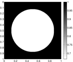
Figure 5. Example 1 of 2D general case. Top: numerical results. Bottom: $c(x)$ (left) and $u(x)+u_{I}(x)$ (right) for the largest $\omega$ value.

$\omega$	$N$	$T_{s}$(sec)	$T_{a}$(sec)	$n_{p}$	$T_{p}$(sec)
1.0e+02	5.7e+03	7.4e-01	3.3e-02	5	2.0e-01
2.0e+02	2.1e+04	2.8e+00	7.6e-02	8	1.1e+00
4.0e+02	7.9e+04	1.8e+01	2.9e-01	8	5.3e+00

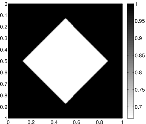
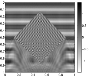
Figure 6. Example 2 of 2D general case. Top: numerical results. Bottom: $c(x)$ (left) and $u(x)+u_{I}(x)$ (right) for the largest $\omega$ value.

Two examples are tested for the 3D case: a smoothed cavity of an $\ell_{2}$ ball and a smoothed cavity of an $\ell_{1}$ ball. The incoming wave is a plane wave pointing downward at frequency $\omega$ and the numerical results are given in Figures 7 and 8.

$\omega$	$N$	$T_{s}$(sec)	$T_{a}$(sec)	$n_{p}$	$T_{p}$(sec)
2.5e+01	6.5e+03	7.1e+00	2.7e-02	4	1.6e-01
5.0e+01	5.5e+04	7.9e+01	3.4e-01	5	2.1e+00
1.0e+02	4.5e+05	1.4e+03	4.1e+00	5	2.3e+01

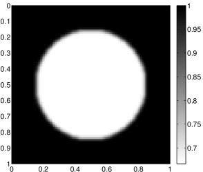
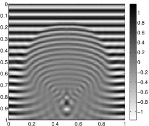
Figure 7. Example 1 of 3D general case. Top: numerical results. Bottom: cross-sections of $c(x)$ (left) and $u(x)+u_{I}(x)$ (right) in the middle of the domain for the largest $\omega$ value.

$\omega$	$N$	$T_{s}$(sec)	$T_{a}$(sec)	$n_{p}$	$T_{p}$(sec)
2.5e+01	3.7e+03	4.9e+00	3.0e-02	4	1.0e-01
5.0e+01	3.1e+04	4.5e+01	1.8e-01	6	1.4e+00
1.0e+02	2.3e+05	7.5e+02	2.1e+00	9	2.3e+01

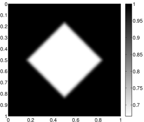
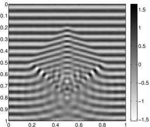
Figure 8. Example 2 of 3D general case. Top: numerical results. Bottom: cross-sections of $c(x)$ (left) and $u(x)+u_{I}(x)$ (right) in the middle of the domain for the largest $\omega$ value.

The results show that the setup and application costs of the preconditioner are lower compared to the ones of the rectangular case. The number of iterations remains essentially independent of the frequency, indicating that the boundary stencils computed randomly provide a sufficiently accurate boundary condition for the solution.

5. Laplace equation

In this section, we consider the 3D Laplace equation with compact potential perturbation, i.e.,

(16) $$(-\Delta+V(x))u(x)=f(x),\quad x\in\mathrm{R}^{3}$$

where $V(x)$ is supported in $\Omega=(0,1)^{3}$ and $u(x)$ decays like $1/|x|$ as $x$ goes to infinity. This can be regarded as a limiting case as $\omega$ goes to zero. The Green’s function is given by

$$G(x)=\frac{1}{4\pi|x|}.$$

Convolving $G(x)$ with (16) gives the Lippmann-Schwinger equation

(17) $$u+G\ast(Vu)=G\ast f.$$

For a potential $V$ that is not too negative, this problem remains elliptic and standard iteration methods such as GMRES converge within a small number of iterations. However, when $V(x)$ is sufficiently negative, the problem loses ellipticity and the iteration number increases dramatically.

As we mentioned, when $\omega$ is finite, PML and ABC offer reasonable approximations to the Sommerfeld radiation condition. When $\omega$ goes to zero, it is not clear how to define analytically a similar local boundary condition at a finite distance for the $1/|x|$ decaying condition. However, the sparsifying preconditioner proposed in Sections 3 and 4 can be applied to (17) without any modification and the resulting operator $B$ offers a good numerical approximation to the $1/|x|$ decaying condition.

5.1. Numerical results

The tests are performed for two examples of $V(x)$: a negative Gaussian function and a smoothed characteristic function of an $\ell_{2}$ ball. In each example, the right hand side $f$ is chosen to be a delta source in $\Omega$ located near the top left corner of the middle cross-section. The potential $V(x)$ is chosen to be negative and proportional to $1/h^{2}$ in order to make sure that the problem loses ellipticity. The numerical results are summarized in Figures 9 and 10.

$\max(|V|)$	$N$	$T_{s}$(sec)	$T_{a}$(sec)	$n_{p}$	$T_{p}$(sec)
5.8e+02	1.2e+04	5.0e+00	4.9e-02	5	2.1e-01
2.3e+03	1.0e+05	9.8e+01	2.8e-01	5	1.8e+00
9.2e+03	8.6e+05	2.1e+03	3.0e+00	6	2.1e+01

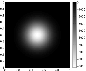
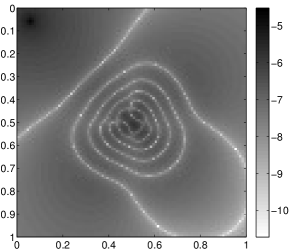
Figure 9. Example 1 of 3D Laplace equation with potential perturbation. Top: numerical results. Bottom: cross-sections of $V(x)$ (left) and $\log_{10}|u(x)|$ (right) in the middle of the domain for the highest resolution test.

$\max(|V|)$	$N$	$T_{s}$(sec)	$T_{a}$(sec)	$n_{p}$	$T_{p}$(sec)
5.8e+02	1.2e+04	5.1e+00	3.8e-02	5	2.9e-01
2.3e+03	1.0e+05	9.8e+01	2.6e-01	7	2.3e+00
9.2e+03	8.6e+05	2.0e+03	2.8e+00	7	2.4e+01

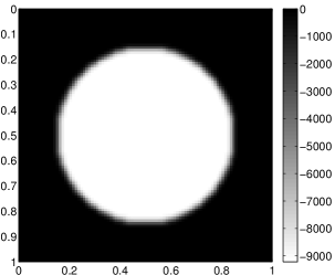
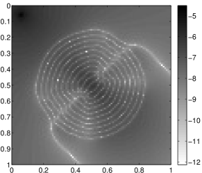
Figure 10. Example 2 of 3D Laplace equation with potential perturbation. Top: numerical results. Bottom: cross-sections of $V(x)$ (left) and $\log_{10}|u(x)|$ (right) in the middle of the domain for the highest resolution test.

The results demonstrate that the number of iterations grows at most logarithmically with the problem size. This implies that the numerically computed boundary condition operator $B$ is a good approximation to the decaying condition of $u$ at infinity.

6. Conclusion

This paper introduces the sparsifying preconditioners for the numerical solution of the Lippmann-Schwinger equation. The main idea is to numerically transform this integral equation into a sparse and localized linear system and then leverage existing efficient sparse linear algebra algorithms. This approach combines the appealing features of the integral equation formulation with the efficiency of the PDE formulations. We discuss the algorithmic details for rectangular and general domains, and extend this approach to the 3D Laplace equation with a potential perturbation.

From the numerical results, we observe that the most of the construction time of the preconditioners is spent on the construction of the nested dissection factorization for the operator in (11). It is possible to replace this step with other solvers such as the sweeping preconditioners [engquist-2011a, engquist-2011b], which are asymptotically more efficient.

Most of the discussion here is in the setting of inhomogeneous acoustic scattering. An immediate task is to use this preconditioner to study problems from electromagnetic and quantum scattering.

This approach is not restricted only to scattering in free space. A future direction is to extend it to fully periodic systems or systems that are periodic in certain directions. This should have direct applications in the study of photonic crystal.

For most numerical methods, the stencil is defined analytically based on the PDE. In the current approach, however, the stencils in the preconditioning operators $A$ and $B$ are defined using the typical behavior of the solution, either deterministically as in Section 3 or randomly as in Section 4. In general, such a practice seems to be fairly unexplored in the field of numerical analysis.