Hint of Lepton Flavour Non-Universality in Meson Decays
Abstract
The LHCb collaboration has recently presented their result on
for the dilepton invariant mass bin GeV2 (). The measurement shows an
intriguing deviation from the Standard Model (SM) prediction.
In view of this, we study model independent New Physics (NP)
explanations of consistent with other measurements involving
transition, relaxing the assumption of lepton universality. We perform a
Bayesian statistical fit to the NP Wilson Coefficients and compare the Bayes
Factors of the different hypotheses in order to quantify their goodness-of-fit. We
show that the data slightly favours NP in the muon sector over NP in the electron
sector.
1 Introduction
While we all hope to see direct evidence of new particles in the upcoming 14 TeV run of the LHC, indirect searches for New Physics (NP) through precision measurements are also extremely important, in particular because of their high sensitivity to Ultra Violet (UV) physics. In fact, the 8 TeV run of the LHC has already seen interesting indirect hints of NP in some of the meson decay modes. The quoted 3.7 deviation observed by the LHCb collaboration last summer Aaij:2013iag ; Aaij:2013qta in one of the angular observables () in the decay for one of the dilepton invariant mass bins ( GeV2) inspired many theorists to come up with NP explanations Descotes-Genon:2013wba ; Altmannshofer:2013foa ; Gauld:2013qba ; Gauld:2013qja ; Datta:2013kja ; Buras:2013qja ; Buras:2013dea ; Altmannshofer:2014cfa . Interestingly enough, very recently the LHCb collaboration has observed a 2.6 deviation in another mode; in the quantity called which is the ratio of the two branching fractions and in the dileptonic invariant mass bin GeV2 () Aaij:2014ora . Note that the branching ratios and are individually predicted with very large hadronic uncertainties () in the SM Bobeth:2007dw . However, their ratio is a theoretically very clean observable and predicted to be if lepton masses are ignored Hiller:2003js . Inclusion of the lepton mass effects changes the prediction only by a tiny amount making it Bobeth:2007dw . This is in contrast to the () anomaly where considerable debate exists surrounding the issue of theoretical uncertainty due to (unknown) power corrections to the factorization framework Jager:2012uw ; Lyon:2014hpa ; Descotes-Genon:2014uoa . Hence, there is a possibility that the observed deviation might be (partly) resolved once these corrections are better understood. On the other hand, the observable is a ratio of two branching fractions which differ only in the flavour of the final state leptons. This makes well protected from hadronic uncertainties in the SM because the strength of the gauge interactions contributing to the short distance physics in the transition are independent of the final state lepton flavour. In fact, this feature remains true even in NP models if the model respects lepton universality. Therefore, the measurement is perhaps pointing towards new short distance physics which is not lepton universal. This motivated us to study possible NP explanations of the measurement (and their consistency with other observables involving the transition) in a model independent way, relaxing the assumption of lepton universality. To this end, we perform a statistical fit to the NP Wilson Coefficients (WC) employing Bayesian inference. In order to quantify and compare the goodness-of-fit of the different hypotheses we also compute their relative Bayes Factors (BFs).
2 Effective Field Theory approach
We base our analysis on the following effective Hamiltonian,
| (1) |
where are the invariant dimension-six operators responsible for the flavour changing transition. The superscript denotes the lepton flavour in the final state . In our notation the short-distance contribution to the WCs is divided into the SM and the NP ones in the following way . In our analysis we consider the subset of operators which are directly responsible for the decay, namely
| (2) | |||||
| (3) | |||||
| (4) |
and the set of chirality flipped operators obtained by interchanging the chiral projectors in the quark current of . The full list of dimension six operators also includes scalar, pseudo-scalar and tensor structures. However, it has been shown that scalar, pseudo-scalar and tensor operators cannot easily give sufficiently large deviations from the SM in the observable once constraints from the other processes are taken into account Alonso:2014csa ; Hiller:2014yaa . Therefore, we will neglect these operators in our analysis. Furthermore, we do not consider NP contributions to the photonic dipole operator as it is lepton flavour blind by construction. In what follows we assume that all the WCs are evaluated at the scale with the corresponding SM contributions given in table 5.
Apart from we also consider data for other processes which proceed via a transition e.g., the branching ratios of the fully leptonic decays and , the inclusive decays and as well as the branching ratio for the semileptonic decay . The SM predictions for these branching fractions and their current experimental values are summarized in table 1. Note that the experimental upper bound on () is larger than the SM prediction by many orders of magnitude. We include this decay mode for completeness but it has no impact on our final results.
| Observable | SM prediction | Measurement | ||
| Bobeth:2012vn | Aaij:2012vr | |||
| Huber:2005ig | Lees:2013nxa | |||
| Bobeth:2013uxa | CMS-PAS-BPH-13-007 | |||
| Huber:2005ig | Lees:2013nxa | |||
| Bobeth:2013uxa | Beringer:1900zz | |||
| Bobeth:2007dw | Aaij:2014ora |
We have not used the branching fraction for the decay from Aaij:2014ora because of its correlation with the measurement. Instead, we have used the value of from a LHCb measurement in Aaij:2012vr . Moreover, we have used the data for only in the low- bin GeV2, the main reason being that a resonance structure in the dilepton invariant mass distribution was observed around GeV2 by the LHCb collaboration last year Aaij:2013pta . This means that even though form factors in the high- region were recently computed from lattice QCD Bouchard:2013mia ; Bouchard:2013eph ; Horgan:2013hoa ; Horgan:2013pva , the theoretical prediction for this observable is affected by non-factorisable hadronic uncertainties. Information coming from high- measurements of this and other observables (such as , etc.) can still be used taking into account conservative estimates of the hadronic uncertanties. We do not expect that the inclusion of such data would change our results drastically, however we expect that the allowed ranges of the WCs would shrink due to the extra observables. We also expect a shift of the best fit points in the direction of the SM values, since these extra measurements are generally in good agreement with the SM predictions.
3 Results
In this section we present our results for the various NP scenarios considered in this paper. As mentioned earlier, we follow a Bayesian statistical approach to quantify our results. The details of our procedure is explained in the Appendix B.
3.1 Single Wilson Coefficient
To start with, we consider only one real NP WC at a time. We will show our results for the WCs both in the standard basis (vector and axial-vector operators for the lepton current) as well as in the chiral basis for the lepton currents. The inclusion of the second set is motivated by the possibility of having the NP WCs generated in an invariant way. This possibility was also highlighted in Hiller:2014yaa .
Our results are summarized in table 2. The 68% confidence level (C.L.) regions of the WCs are shown in the second column, the best fit values are shown in the third column while the last column shows the BF for each hypothesis taking the same for the -only hypothesis as the reference value. More precisely, the BF for the hypothesis with NP in the WC is defined as
| (5) |
where is the likelihood function and is our choice of prior for the WC , which we assume to be a flat distribution in the range [-10, 10].
| Hypothesis | Fit | Best fit | BF |
| [-3.1,-0.7] | -1.6 | ||
| [-1.9,-0.8] | -1.3 | ||
| [0.7,1.3], [7.5,8.1] | 1.0 | ||
| [0.2,0.7] | 0.5 | ||
| [0.1,0.8] | 0.5 | ||
| [-0.8,-0.4] | -0.6 | ||
| [-0.4,0.3] | -0.1 | ||
| [-0.2,-0.6] | -0.4 | ||
| [-8.4,-8.4], [0.6,2.1] | 1.3 | ||
| [0.8,1.9] | 1.3 | ||
| [-1.6,-0.7], [9.5,10.0] | -1.1 | ||
| [-1.7,-0.7] | -1.1 | ||
| [-2.4,-1.4], [2.2,3.4] | -1.9 | ||
| [0.3,1.1] | 0.6 | ||
| [-2.6,-1.5], [2.2,3.2] | -2.0 | ||
| [0.4,0.9] | 0.7 | ||
| = | [-4.3,-1.1] | -2.2 | |
| = | [0.3,1.2], [7.6,8.4] | 0.8 | |
| SM |
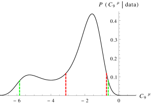
In Figure 1 we show the posterior probabilities for the only and only hypotheses as examples.
We now discuss some general features of our results shown in table 2. Clearly, the hypothesis with non-zero is the most favoured by the data as it offers the largest BF. The NP scenario also does quite well. As does not contribute to the decay (whose experimental central value is now slightly lower than the SM prediction), its BF is reduced to some extent. The extremely low BF for the case is due to a tension between and and . It can be seen from the expressions of these two observables (see Appendices A.1 and A.4 ) that the experimental value for prefers while the measured branching ratio for prefers the opposite. The hypotheses (which correspond to the operator directions and ) are also strongly disfavoured because they generate which is in tension with experiment. The other chiral operator (our hypothesis ) turns out to be the best among the four chiral operators. This case was also considered in Ref. Hiller:2014yaa in the context of their model independent analysis as well as a specific leptoquark model. In their analysis they quote as a benchmark point which is in fact consistent with our 68% CL range in table 2.
 |
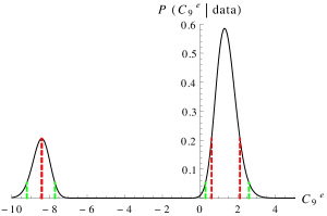 |
As far as NP in the electron sector is concerned, all the hypotheses give similar BFs (at most a factor 4 between the best and the worst). This can be understood by the fact that the measurements with electrons in final states have a larger experimental error than those with muons in the final state. Note also that there are a few cases with multiple solutions (because the rates are quadratically dependent on the WCs), some of them with very large NP contributions (see for example ). Including other observables (for example those in the decay ) will certainly modify this picture.
The scenario was also considered in the Ref. Hiller:2014yaa . Although their estimate is compatible with the 68% CL region from our fit, its BF is the worst among the hypotheses with NP in the electron sector.
The highest BFs are obtained for hypotheses with NP in the muon sector. In our fit, this finding is driven by the observables and , for which the dimuon channel measurements are each lower (at more than 1 level) than the SM predictions, while the electron channel measurement is in good agreement with the SM. Hence our fit finds a slight preference for NP in the muon sector. For example, a negative value for will lower the predictions for both and compared to the SM while keeping at its SM value.
Finally, we show our results for the two lepton universal cases = and = (see the last but one row in table 2). It can be seen that the BF for both these two cases are rather low compared to most of the non-universal NP scenarios in particular, the -only and -only hypotheses.
3.2 Combination of two Wilson Coefficients at a time
In this section we allow the possibility of having NP in two WCs simultaneously and study the consequences. Here we do not consider all the possible combinations of the WCs, rather, we take the few best cases from table 2 and consider their combinations. Our results are summarized in table 3. The 68% range of a parameter is obtained after marginalizing over the other parameter.
The results of our analysis show that, in general, there is no particular gain in considering NP effects in two WCs at the same time, this is more marked in the case of the chiral operators.
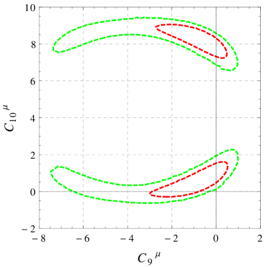
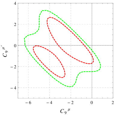
Among the hypothesis of NP in two WCs, the largest BF is obtained for the pair . The 2-dimensional posterior distribution for this scenario is shown in the left panel of figure 2. Similarly, the posterior probability distribution for the NP scenario with both and is shown is the right panel of figure 2. It can be seen that the data is consistent with no NP in .
| Hypothesis | Fit | Best fit | BF |
| [-1.9,0.3] | -0.6 | ||
| [-0.1,0.9], [8.0,8.8] | 0.4 | ||
| [-4.2,-1.2] | -2.8 | ||
| [-1.7,1.2] | -0.3 | ||
| [-4.2,-1.4] | -2.6 | ||
| [-7.4,-5.9], [-1.3,0.2] | -6.6 | ||
| [-1.0,0.4] | -0.7 | ||
| [-0.5,0.4], [-8.2,-7.4] | -0.1 | ||
| [-0.7,-0.4] | -0.5 | ||
| [-1.2,1.6] | -0.2 | ||
| [0.1,0.9] | 0.5 | ||
| [0.3,1.1] | 0.6 | ||
| [0.1,0.9] | 0.5 | ||
| [-2.4,-1.5], [2.2,3.4] | 2.8 |
 |
 |
 |
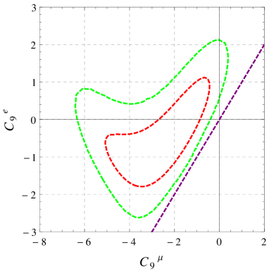 |
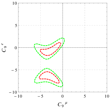
The posterior probability for the hypothesis with both and turned on is shown in figure 3. In the left panel we show both the allowed regions, while in the right panel we show a zoomed in version of the region close to the SM point . Figure 3 clearly shows that the data prefers NP in the muon sector over NP in the electron sector. Moreover, NP with lepton flavour universality (shown by the the dashed purple line) is disfavoured by more than 95% C.L.
3.3 Including the data on
The latest LHCb measurement of the decay distribution in has seen interesting deviations in several observables from their SM predictions Aaij:2013iag ; Aaij:2013qta . These deviations were most pronounced in two of the so-called optimized observables (where the hadronic uncertainties are expected to cancel to a good extent) and in the low- region Descotes-Genon:2013vna . Soon after the LHCb result was published, it was shown in Descotes-Genon:2013wba that a good fit to all the data can be obtained by having a negative contribution in the range to the WC . A similar conclusion was also reached by two other groups Altmannshofer:2013foa ; Beaujean:2013soa . The fit done in Altmannshofer:2013foa found a need for a NP contribution (similar to in magnitude but with opposite sign) also to the chirally flipped operator . As discussed in section 3.2 this is now in tension with the measurement of (assuming the presence of NP only in the muon sector).
Note that the issue of hadronic uncertainties, in particular the role of long-distance loops still remains unclear, see Descotes-Genon:2014uoa and the references therein for a recent discussion. Thus, the jury is still out on whether NP has already been seen in these measurements. Despite this uncomfortable situation, several NP interpretations of the LHCb data have been proposed Gauld:2013qja ; Datta:2013kja ; Buras:2013qja and it would be interesting to see whether the measurement can be reconciled with the data. With this motivation, in this section we combine the result of Descotes-Genon:2013wba with our analysis.
| Hypothesis | Fit | Best Fit | BF |
| [-1.9,-1.3] | -1.6 | ||
| [-1.9,-1.3] | -1.6 | ||
| [-7.7,-6.6], [-0.7,0.6] | -0.1 | ||
| [-1.8,-1.4] | -1.6 | ||
| [-0.4,0.5], [8.3,9.3] | 8.7 | ||
| [-1.8,-1.3] | -1.5 | ||
| [-0.9,1.5] | -0.1 | ||
| [-1.9,-1.3] | -1.6 | ||
| [-8.2,-7.8], [-0.3,0.3] | 0.0 |
We follow an approximate procedure (see Appendix B for more details) which allows us to use their result where NP only in and was considered, see their eq. 4. Note that, although the analysis in Descotes-Genon:2013wba was performed assuming lepton universality their results can, to a very good approximation, be taken as valid only for the muonic WCs. This allows us to safely use their result with NP in and any operator in the electron sector. As we do not consider NP in the dipole operator in this paper, is set to its SM value (which is consistent with the 68% C.L. region of Descotes-Genon:2013wba ).
 |
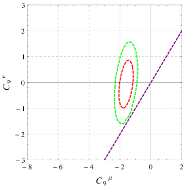 |
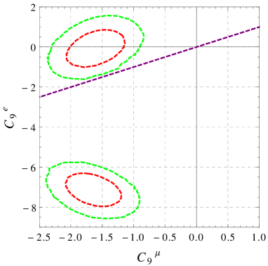
The result of our fit is reported in table 4. In the first row we show the result when only is turned on while in the following rows we allow NP in the electron sector in addition to . We notice that the range for preferred by the analysis of Descotes-Genon:2013wba is confirmed even with the inclusion of our observables. Allowing the possibility of NP in the electron sector makes things slightly better (increases the BF by roughly a factor of 3), except for the scenario of the last row of the table where the BF remains almost the same. The posterior probability distribution for the - hypothesis is shown in figure 4. Similar to figure 3, in the left panel both the allowed regions are shown while in the right panel only the region close to the SM point is shown. Again, the preference for lepton flavour non-universal NP is very clear. The data is consistent with no NP in the electron sector but demands a rather large NP in the muon sector. A comparison of the figure in the right panel with that in figure 3 will also show the constraining power of the data. We warn the readers that the BFs in the table 4 should not be compared with those in the previous section but should only be compared within table 4. This is because the analysis in this section uses different set of information than those in the previous section. Also, we are combining our analysis with that in Descotes-Genon:2013wba in a very simplified way. We report the BFs just to show that the data does not show a strong preference for any particular kind of NP in the electron sector; many of them do equally well.
4 Summary and conclusions
The flavour changing process is responsible for many rare decays such as , , and . These decays, being extremely rare in the SM, are very powerful probes of NP. The LHCb collaboration already made significant progress last year by measuring most of the observables in the full three angle distribution of the decay . Interesting deviations from the SM predictions were seen in a few of the so-called “form-factor independent” or optimized observables. Although several NP explanations of these deviations were put forward, firm confirmation of NP in these observables is not yet possible due to the hadronic uncertainties which are not completely understood. The deviation in , although not yet statistically significant, is worthy of attention because the ratio is essentially free of hadronic uncertainties in the SM. Moreover, any lepton flavour blind new short distance physics would predict and hence, the confirmation of this deviation would clearly point towards lepton flavour non-universal NP. This has motivated us to study model independent NP explanations of the measurement of considering various observables involving a transition. To this end, we have performed a Bayesian statistical analysis of the various NP scenarios. We have also quantified the goodness-of-fit of these NP hypotheses by computing and comparing their Bayes Factors.
We first performed a fit without including the data on . Our results for the hypothesis of NP in one (two) WC(s) at a time are summarized in Table 2 (3). In the muon sector, among the fits to a single WC in the standard basis, only and have large BFs while among the chiral operators, the hypothesis of NP in gives the highest BF. In the electron sector all the NP hypotheses give comparable BFs, although worse than the scenarios with or . Even without the inclusion of the data, our fit shows a slight preference towards the hypothesis of NP in the di-muon sector. However it should be noted that large NP effects in the electron sector are not excluded and in the future, with more precise measurements, the situation could change. We further show that the lepton flavour universal NP scenarios for example, or have rather low BFs and hence they are disfavoured.
When two NP WCs are turned on simultaneously, the situation does not particularly improve. We have shown a few posterior distributions in figures 2 and 3 and we notice that for the – hypothesis the lepton flavour universal case is disfavoured at more than 95% C.L. We continued in section 3.3 by including also the data on . We employed a simplified procedure (explained in appendix B) to combine part of the results from Descotes-Genon:2013wba with our observables. We observed that the allowed range of obtained in Descotes-Genon:2013wba remains consistent with the data. Our analysis also showed that the data is consistent with no NP in the electron sector.
A global analysis including the final states with tau leptons would be very interesting once more data are available. In fact, the possibility of large enhancements in many of the modes were already discussed in the context of like-sign dimuon asymmetry seen at the Tevatron, see for example Dighe:2010nj ; Dighe:2012df .
Acknowledgments:
DG is supported by the European Research Council under the European Union’s Seventh Framework Programme (FP/2007-2013) / ERC Grant Agreement n.279972. DG would like to thank Prof. Benjamin Allanach for his hospitality in DAMTP, University of Cambridge where this project was envisaged. DG also thanks Prof. Michael Spannowsky and the CERN theory division for their hospitalities in IPPP Durham and CERN respectively where part of this work was carried out. Discussion with Prof. Luca Silvestrini is also gratefully acknowledged. MN and SR are supported by STFC. MN and SR want to thank Ben Allanach for useful discussions on Bayesian statistics. Thanks to Diego Guadagnoli and David Straub for helpful comments.
Appendix A Details of the analysis
A.1
The branching ratio for the decay in the low- region can be written as Bobeth:2007dw ; Alok:2010zd ; Alok:2011gv ; Khodjamirian:2010vf ,
| (6) |
where the numerical values for , and are given by,
In order to obtain these numbers we have used the form factor parametrization given in Khodjamirian:2010vf . The values of the form factor parameters , , and are given in table 5. As far as the uncertainties in these parameters are concerned, for and we have taken asymmetric gaussian priors in the fit. For the other two parameters and , we have fixed them to their respective central values and the associated uncertainties are taken into account by rescaling the experimental error in by
| (7) |
(taking conservatively the values , and ) . We made this (conservative) approximation in order to reduce the computational time in the evaluation of the posterior distributions for the WCs and avoid some numerical instabilities. We have followed the same prescription also for the branching ratio of . The theoretical uncertainties coming from and in the two observables and have been assumed to be independent for simplicity.
A.2
The expression for can be derived using the result given in the previous subsection. Here we give a simplified formula which can be useful for analytic understanding of our results. Observing the fact that and also that the NP in is severely constrained by the measured branching ratio of , the expression of can be approximated by,
| (8) |
This simplified expression clearly shows that the theoretical error in is very small even in the presence of NP. Note that in our numerical fit we have used the full expression of with all the form factor dependent terms.
A.3
The branching ratio for the inclusive decay in the low- region can be written as DescotesGenon:2011yn
| (9) | |||||
We took the theoretical error into account by taking a gaussian prior for a parameter called and marginalizing over it, with its central value and standard deviation given by 15.86 and 1.51 respectively.
A.4
The branching ratio for the leptonic decays and can be written as
| (10) | |||||
| (11) |
Here we have used the SM value of as our input parameter instead of the meson decay constant and the CKM matrix elements. We took the theoretical error on this into account by taking a gaussian prior for and marginalizing over it, using values from Bobeth:2013uxa :
Appendix B Statistical procedure
In this appendix we briefly describe the statistical procedure that has been followed in this work. Our aim is to construct the posterior probability distributions (p.d.f.) for a set of WCs that we denote collectively by , for example .
The theoretical prediction for a given observable will be denoted by and it will depend on as well as a set of input parameters , for example CKM matrix elements, form factors, masses of the particles etc. The inputs are either experimentally measured quantities or theoretically calculated parameters with some uncertainties. In order to take into account these uncertainties we have to attach a probability distribution to each input .
The measured observables will be assumed to be distributed according to a Normal distribution with mean value and standard deviation . The generalization to distributions other than the Normal distribution is straightforward.
If one has a set of observables (), following the Bayesian approach111In particular, in the same spirit of section 3 of Ciuchini:2000de ., the p.d.f. of the WCs can be written as
| (12) |
Let us now split the observables into two sets, and where the second (first) set refers to the observables (without) involving the decay . In a similar way, we split the set of inputs into three sets where () are input parameters entering the set of observables () exclusively and are the inputs which are common to both the sets of observables. The expression for the p.d.f. now reduces to
| (13) | |||||
Now we would like to find the conditions such that the two sets of observables “factorize”. In that case, we will be able to use the results of Descotes-Genon:2013wba instead of redoing the full analysis. The factorization is possible if the common set of inputs has small uncertainty compared to the other sources of uncertainties. If that is true then one can write to a very good approximation and the p.d.f. reduces to
| (14) |
where is the result of a Bayesian analysis considering only the global analysis of the decay . Using the result of Descotes-Genon:2013wba in their section 3.2, we assume that
| (15) |
with
| (16) |
These values are inferred from eq. (4) of Descotes-Genon:2013wba . We finally remark that although Ref. Descotes-Genon:2013wba considered the observable under the assumption of lepton universality, we interpret that as and remove the experimental data on (our table 1) from our fit for consistency. We have also not used the data on since that was also already included in the fit of Ref. Descotes-Genon:2013wba .
Appendix C Input parameters
| Parameters | Value | |
| GeV-2 | Beringer:1900zz | |
| Beringer:1900zz | ||
| MeV | Beringer:1900zz | |
| MeV | Beringer:1900zz | |
| GeV | Khodjamirian:2010vf | |
| GeV | Beringer:1900zz | |
| GeV | Beringer:1900zz | |
| sec. | Beringer:1900zz | |
| Charles:2004jd | ||
| GeV | Beringer:1900zz | |
| Wilson coefficients | ||
| -0.319 | Khodjamirian:2010vf | |
| 4.228 | Khodjamirian:2010vf | |
| -4.410 | Khodjamirian:2010vf | |
| Form factors | ||
| Khodjamirian:2010vf | ||
| Khodjamirian:2010vf | ||
| Khodjamirian:2010vf | ||
| Khodjamirian:2010vf | ||
References
- (1) LHCb Collaboration Collaboration, R. Aaij et al., Differential branching fraction and angular analysis of the decay , JHEP 1308 (2013) 131, [arXiv:1304.6325].
- (2) LHCb collaboration Collaboration, R. Aaij et al., Measurement of Form-Factor-Independent Observables in the Decay , Phys.Rev.Lett. 111 (2013), no. 19 191801, [arXiv:1308.1707].
- (3) S. Descotes-Genon, J. Matias, and J. Virto, Understanding the Anomaly, Phys.Rev. D88 (2013), no. 7 074002, [arXiv:1307.5683].
- (4) W. Altmannshofer and D. M. Straub, New physics in ?, Eur.Phys.J. C73 (2013) 2646, [arXiv:1308.1501].
- (5) R. Gauld, F. Goertz, and U. Haisch, On minimal Z’ explanations of the anomaly, Phys.Rev. D89 (2014) 015005, [arXiv:1308.1959].
- (6) R. Gauld, F. Goertz, and U. Haisch, An explicit Z’-boson explanation of the anomaly, JHEP 1401 (2014) 069, [arXiv:1310.1082].
- (7) A. Datta, M. Duraisamy, and D. Ghosh, Explaining the data with scalar interactions, Phys.Rev. D89 (2014) 071501, [arXiv:1310.1937].
- (8) A. J. Buras and J. Girrbach, Left-handed Z’ and Z FCNC quark couplings facing new data, JHEP 1312 (2013) 009, [arXiv:1309.2466].
- (9) A. J. Buras, F. De Fazio, and J. Girrbach, 331 models facing new data, JHEP 1402 (2014) 112, [arXiv:1311.6729].
- (10) W. Altmannshofer, S. Gori, M. Pospelov, and I. Yavin, Dressing - in Color, Phys.Rev. D89 (2014) 095033, [arXiv:1403.1269].
- (11) LHCb collaboration Collaboration, R. Aaij et al., Test of lepton universality using decays, arXiv:1406.6482.
- (12) C. Bobeth, G. Hiller, and G. Piranishvili, Angular distributions of decays, JHEP 0712 (2007) 040, [arXiv:0709.4174].
- (13) G. Hiller and F. Kruger, More model independent analysis of processes, Phys.Rev. D69 (2004) 074020, [hep-ph/0310219].
- (14) S. Jäger and J. Martin Camalich, On at small dilepton invariant mass, power corrections, and new physics, JHEP 1305 (2013) 043, [arXiv:1212.2263].
- (15) J. Lyon and R. Zwicky, Resonances gone topsy turvy - the charm of QCD or new physics in ?, arXiv:1406.0566.
- (16) S. Descotes-Genon, L. Hofer, J. Matias, and J. Virto, On the impact of power corrections in the prediction of observables, arXiv:1407.8526.
- (17) R. Alonso, B. Grinstein, and J. M. Camalich, gauge invariance and the shape of new physics in rare decays, arXiv:1407.7044.
- (18) G. Hiller and M. Schmaltz, and future BSM opportunities, arXiv:1408.1627.
- (19) C. Bobeth, G. Hiller, and D. van Dyk, General Analysis of Decays at Low Recoil, Phys.Rev. D87 (2013) 034016, [arXiv:1212.2321].
- (20) LHCb Collaboration Collaboration, R. Aaij et al., Differential branching fraction and angular analysis of the decay, JHEP 1302 (2013) 105, [arXiv:1209.4284].
- (21) T. Huber, E. Lunghi, M. Misiak, and D. Wyler, Electromagnetic logarithms in anti-B X(s) l+ l-, Nucl.Phys. B740 (2006) 105–137, [hep-ph/0512066].
- (22) BaBar Collaboration Collaboration, J. Lees et al., Measurement of the B-¿Xsl+l- branching fraction and search for direct CP violation from a sum of exclusive final states, Phys.Rev.Lett. 112 (2014) 211802, [arXiv:1312.5364].
- (23) C. Bobeth, M. Gorbahn, T. Hermann, M. Misiak, E. Stamou, et al., in the Standard Model with Reduced Theoretical Uncertainty, Phys.Rev.Lett. 112 (2014) 101801, [arXiv:1311.0903].
- (24) CMS and LHCb Collaborations Collaboration, Combination of results on the rare decays from the CMS and LHCb experiments, Tech. Rep. CMS-PAS-BPH-13-007. CERN-LHCb-CONF-2013-012, CERN, Geneva, Jun, 2014.
- (25) Particle Data Group Collaboration, J. Beringer et al., Review of Particle Physics (RPP), Phys.Rev. D86 (2012) 010001.
- (26) LHCb collaboration Collaboration, R. Aaij et al., Observation of a resonance in decays at low recoil, Phys.Rev.Lett. 111 (2013), no. 11 112003, [arXiv:1307.7595].
- (27) HPQCD Collaboration Collaboration, C. Bouchard, G. P. Lepage, C. Monahan, H. Na, and J. Shigemitsu, Standard Model Predictions for with Form Factors from Lattice QCD, Phys.Rev.Lett. 111 (2013), no. 16 162002, [arXiv:1306.0434].
- (28) HPQCD Collaboration Collaboration, C. Bouchard, G. P. Lepage, C. Monahan, H. Na, and J. Shigemitsu, Rare decay form factors from lattice QCD, Phys.Rev. D88 (2013), no. 5 054509, [arXiv:1306.2384].
- (29) R. R. Horgan, Z. Liu, S. Meinel, and M. Wingate, Lattice QCD calculation of form factors describing the rare decays and , Phys.Rev. D89 (2014) 094501, [arXiv:1310.3722].
- (30) R. R. Horgan, Z. Liu, S. Meinel, and M. Wingate, Calculation of and observables using form factors from lattice QCD, Phys.Rev.Lett. 112 (2014) 212003, [arXiv:1310.3887].
- (31) S. Descotes-Genon, T. Hurth, J. Matias, and J. Virto, Optimizing the basis of observables in the full kinematic range, JHEP 1305 (2013) 137, [arXiv:1303.5794].
- (32) F. Beaujean, C. Bobeth, and D. van Dyk, Comprehensive Bayesian Analysis of Rare (Semi)leptonic and Radiative B Decays, Eur.Phys.J. C74 (2014) 2897, [arXiv:1310.2478].
- (33) A. Dighe, A. Kundu, and S. Nandi, Enhanced lifetime difference and anomalous like-sign dimuon charge asymmetry from new physics in , Phys.Rev. D82 (2010) 031502, [arXiv:1005.4051].
- (34) A. Dighe and D. Ghosh, How large can the branching ratio of be ?, Phys.Rev. D86 (2012) 054023, [arXiv:1207.1324].
- (35) A. K. Alok, A. Datta, A. Dighe, M. Duraisamy, D. Ghosh, et al., New Physics in : CP-Conserving Observables, JHEP 1111 (2011) 121, [arXiv:1008.2367].
- (36) A. K. Alok, A. Datta, A. Dighe, M. Duraisamy, D. Ghosh, et al., New Physics in : CP-Violating Observables, JHEP 1111 (2011) 122, [arXiv:1103.5344].
- (37) A. Khodjamirian, T. Mannel, A. Pivovarov, and Y.-M. Wang, Charm-loop effect in and , JHEP 1009 (2010) 089, [arXiv:1006.4945].
- (38) S. Descotes-Genon, D. Ghosh, J. Matias, and M. Ramon, Exploring New Physics in the C7-C7’ plane, JHEP 1106 (2011) 099, [arXiv:1104.3342].
- (39) M. Ciuchini, G. D’Agostini, E. Franco, V. Lubicz, G. Martinelli, et al., 2000 CKM triangle analysis: A Critical review with updated experimental inputs and theoretical parameters, JHEP 0107 (2001) 013, [hep-ph/0012308].
-
(40)
CKMfitter Group Collaboration, J. Charles et al., CP violation and
the CKM matrix: Assessing the impact of the asymmetric factories, Eur.Phys.J. C41 (2005) 1–131,
[hep-ph/0406184].
Updated results and plots available at: http://ckmfitter.in2p3.fr.