Tensor Numerical Methods for High-dimensional PDEs: Basic Theory and Initial Applications

Abstract

We present a brief survey on the modern tensor numerical methods for multidimensional stationary and time-dependent partial differential equations (PDEs). The guiding principle of the tensor approach is the rank-structured separable approximation of multivariate functions and operators represented on a grid. Recently, the traditional Tucker, canonical, and matrix product states (tensor train) tensor models have been applied to the grid-based electronic structure calculations, to parametric PDEs, and to dynamical equations arising in scientific computing. The essential progress is based on the quantics tensor approximation method proved to be capable to represent (approximate) function related $d$-dimensional data arrays of size $N^{d}$ with log-volume complexity, $O(d\log N)$. Combined with the traditional numerical schemes, these novel tools establish a new promising approach for solving multidimensional integral and differential equations using low-parametric rank-structured tensor formats. As the main example, we describe the grid-based tensor numerical approach for solving the 3D nonlinear Hartree-Fock eigenvalue problem, that was the starting point for the developments of tensor-structured numerical methods for large-scale computations in solving real-life multidimensional problems. We also discuss a new method for the fast 3D lattice summation of electrostatic potentials by assembled low-rank tensor approximation capable to treat the potential sum over millions of atoms in few seconds. We address new results on tensor approximation of the dynamical Fokker-Planck and master equations in many dimensions up to $d=20$. Numerical tests demonstrate the benefits of the rank-structured tensor approximation on the aforementioned examples of multidimensional PDEs. In particular, the use of grid-based tensor representations in the reduced basis of atomics orbitals yields an accurate solution of the Hartree-Fock equation on large $N\times N\times N$ grids with a grid size of up to $N=10^{5}$.

1 Introduction

In the recent years, the tensor numerical methods were recognized as the basic tool to render numerical simulations in higher dimensions tractable. The guiding principle of the tensor numerical methods is the reduction of the computational process onto a low parametric rank-structured manifold by using an approximation of multivariate functions and operators, that relies on a certain separation of variables. Possible applications of tensor numerical methods include high-dimensional problems arising in material- and bio-sciences, computational quantum chemistry, stochastic modeling and uncertainty quantification, dynamical systems, machine learning, financial mathematics, etc.

In the following discussion a tensor of order $d$ and mode size $N$, or briefly $N$-$d$ tensor, is considered as a function on a $d$-fold product index set, $\textsf{{A}}:I^{\otimes d}\to\mathbb{R}$ with $I^{\otimes d}=I\times\cdot\cdot\cdot\times I$, and $I=\{1,...,N\}$. In the traditional grid-based numerical techniques for $d$-dimensional PDEs the parameter $N$ can be associated with the univariate grid size. The representation of arising $N$-$d$ tensors (coefficient vectors) requires a storage size that is exponential in $d$, $N^{d}$, which causes severe computational difficulties, often called the “curse of dimensionality“ [11].

A class of methods which lead to linear scaling in the dimension are distinctly linked with the principle of separation of variables. The multi-linear tensor decompositions based on the Tucker and canonical models have long since been used as a tool for data processing in the computer science community (e. g. PCA type methods), and applied to multidimensional experimental data in chemometrics, psychometrics and in signal processing, see a comprehensive bibliography in [83]. The remarkable approximating properties of the Tucker and canonical decomposition for wide classes of function related tensors were revealed in [64, 71], promoting its usage as a tool for the numerical treatment of multidimensional problems in numerical analysis. An introductory description of traditional tensor formats with the focus on tensor-structured numerical methods for the calculation of multidimensional functions and operators is presented in [56, 69, 70]. Moreover, the canonical tensor representations obtained by sinc approximations on a class of analytic multivariate functions have been proven to provide fast exponential convergence in the separation rank [35, 45, 64, 125].

First successes in the rank-structured tensor calculations of multivariate functions and operators in the Hartree-Fock equation originated the grid-based tensor numerical methods in scientific computing [72, 73, 56, 61, 59, 62, 63, 124]. Combined with the matrix product states (MPS) techniques developed in the physics community, [123, 118, 121, 119, 106], including its particular form, the tensor train (TT) format [102, 98], and with the newly developed quantized tensor approximation of discretized functions [67] and operators [99], these methods boiled up to a powerful tool for the numerical analysis in higher dimensions. Concerning computational quantum chemistry, the real space numerical methods combined with FEM or plane waves approximations have become attractive in (post) Hartree-Fock and DFT calculations as the possible alternative to traditional approaches [87, 47, 16, 20, 32, 17, 34, 107].

Literature surveys on the most frequently used tensor formats can be found in [69, 110, 42, 39]. In addition, methods of multilinear algebra and nonlinear tensor approximation have been discussed, see [1, 72, 102, 70, 67, 37] and references therein. The numerical cost of basic multilinear algebra operations on formatted $N$-$d$ tensors usually scales linearly in $d$, but could be polynomial in the mode size $N$. This leads to essential limitations, since the high precision numerical simulations might require $N^{\otimes d}$-grids with large mode size $N\sim 10^{4},...,10^{6}$.

The new paradigm of the quantics-TT (QTT) approximation for a class of discretized functions, as introduced and rigorously justified in [66, 67], leads to a data compression with $O(\log N)$ complexity scaling. In this way the QTT approximation applies to the quantized image of the target discrete function, obtained by its isometric folding transformation to the higher dimensional quantized tensor space. For example, a vector of size $N=q^{L}$ ($q=2,3,...$) can be successively reshaped by a $q$-adic folding to an $L$-fold tensor in $\bigotimes_{j=1}^{L}\mathbb{R}^{q}$ of the irreducible mode size $n=q$ (quantum of information), then the low-rank approximation in the canonical or TT formats can be applied consequently.

The principal question arises: how can the folding of a vector to a higher dimensional tensor in $\bigotimes_{j=1}^{L}\mathbb{R}^{q}$ lead to the essential data compression using representations in low-rank tensor formats and, hence, to the efficient $O(\log N)$-approximation method? The constructive answer is formulated by the QTT approximation theory proven for the basic classes of function related tensors: The TT-rank of quantized exponential, trigonometric, and polynomial $N$-vectors remains constant, that is independent of $N$ [66, 67]. As a simple corollary, it was shown that the QTT approximation provides exponential convergence in the QTT-rank for a class of analytic function related $N$-vectors and $N$-$d$ tensors, which are well representable in terms of the aforementioned functional classes. These beneficial approximation features allow to understand why the computation in quantized tensor spaces may lead to a log-volume complexity, $O(d\log N)$. Further QTT approximation results for functional vectors can be found in [79, 38, 100, 25, 104, 23, 60, 54, 62].

The important point for solving PDEs is that typical integral and elliptic differential operators also admit the low QTT-rank representation. It was found in [99] by numerical tests that in some cases the dyadic reshaping of an $2^{L}\times 2^{L}$ matrix leads to a small TT-rank of the reshaped operator. An explicit low-rank QTT representation of the matrix exponential as well as the discrete quantized Laplacian and its inverse were derived in [77, 78, 51].

We summarize that the idea of quantized tensor approximation in $d\log N$-complexity allows a fast functional and operator calculus on very large discretization grids (practically unlimited grid size). This opens a way to the efficient computation of $d$-dimensional integrals with controllable accuracy, the representation of discrete elliptic operators and their inverse, as well as various linear and bilinear mappings on tensors of order $d$, thus making the decisive step toward tractable numerical methods for multi-dimensional PDEs.

As a matter of fact the concept of low-rank separable representation of multidimensional functions and operators in combination with properly modified traditional numerical schemes, and with well developed algebraic tools for formatted tensors has penetrated into the new branch of numerical analysis in the form of tensor-structured numerical methods (TNM) for solving multi-dimensional PDEs. The main ingredients of TNMs for PDEs include:

• FEM or spectral discretization of $d$-dimensional PDEs in tensor product Hilbert spaces

• Numerical multilinear algebra of rank-structured tensors

• Approximate grid-based tensor calculus of multivariate functions and operators in low-parametric tensor formats

• Quantized tensor approximation

• Tensor truncated iterative methods for solving discrete systems of stationary and time dependent $d$-dimensional PDE.

This survey is merely an attempt to outline the main results on TNMs for multidimensional PDEs obtained in the recent years by the author and in collaborations, which have been presented at the Summer School CEMRACS-2013, “Modeling and simulation of complex systems: Stochastic and deterministic approaches”, CIRM, Marseille-Luminy, France, 22-26.07.2013. We mainly focus on the recently developed grid-based tensor numerical methods for solving the 3D nonlinear Hartree-Fock eigenvalue problem, including the new method of fast lattice summation of electrostatic potentials by the assembled low-rank tensor approximation, and also discuss the tensor method of simultaneous $(x,t)$-approximation in TT/QTT formats for the dynamical Fokker-Planck and master equations in many dimensions up to $d=20$.

Several important applications of tensor numerical methods remain beyond the scope of this review. They include multidimensional preconditioning [65, 3] and solution of linear systems [86, 28, 120, 30, 29, 12], parametric/stochastic PDEs [93, 81, 76, 27, 13], greedy algorithms [90, 9, 19, 33], PGD model reduction methods [2, 31, 116], super-fast FFT, convolution and wavelet transforms [24, 52, 75], tensor-product interpolation and cross approximation [103, 8, 109, 5], integration of singular or highly oscillating functions [80], control problems [115], complexity theory [4, 21], etc.

The rest of the manuscript is structured as follows. Section 2 introduces the basic rank-structured tensor formats with a focus on the quantized tensor representation of functions and operators. Section 3 describes the main building blocks in the construction and justification of TNMs for the solution of the Hartree-Fock equation in ab initio electronic structure calculations, and for the tensor approximation of the real-time high-dimensional stochastic multiparticle dynamics governed by master equations. Section 4 concludes the paper and outlines challenging problems for future research.

2 Rank-structured tensor approximation

In this section we present a short description of the basic additive and multiplicative tensor formats. These formats allow low-parametric function and operator representations by a nonlinear mapping onto the rank-structured tensor manifolds.

2.1 Basic tensor formats for representation of functions and operators

A tensor of order $d$, further called $N$-$d$ tensor, is defined as an element of finite dimensional tensor-product Hilbert space of the $d$-fold, $N_{1}\times...\times N_{d}$ real/complex-valued arrays, $\mathbb{W}_{\bf n}\equiv\mathbb{W}_{{\bf n},d}=\bigotimes_{\ell=1}^{d}X_{\ell}$, where $X_{\ell}=\mathbb{R}^{N_{\ell}}$ or $X_{\ell}=\mathbb{C}^{N_{\ell}}$, and ${\bf n}=(N_{1},...,N_{d})$. An element of $\mathbb{W}_{\bf n}$ can be represented entrywise by

$$\textsf{{A}}=[\textsf{A}(i_{1},...,i_{d})]\equiv[\textsf{A}_{i_{1},...,i_{d}}]\quad\mbox{with}\quad i_{\ell}\in I_{\ell}:=\{1,...,N_{\ell}\}.$$

We confine ourselves to the case of real-valued tensors in $\mathbb{W}_{\bf n}=\mathbb{R}^{\cal I}$, ${\cal I}=I_{1}\times...\times I_{d}$, though all the constructions can be extended to the case of complex-valued tensor-product Hilbert space, $\mathbb{W}_{{\bf n}}=\mathbb{C}^{\cal I}$. The Euclidean scalar product, $\left\langle\cdot,\cdot\right\rangle:\mathbb{W}_{\bf n}\times\mathbb{W}_{\bf n}\to\mathbb{R}$, is defined by

$$\left\langle\textsf{{A}},\textsf{{B}}\right\rangle:=\sum_{{\bf i}\in{\cal I}}\textsf{A}({\bf i})\textsf{B}({\bf i}),\quad\textsf{{A}},\textsf{{B}}\in\mathbb{W}_{\bf n},$$

that merely identifies tensors with multi-indexed Euclidean vectors. Any particular tensor can be associated with a function of a discrete variable, $\textsf{{A}}:I_{1}\times...\times I_{d}\to\mathbb{R}$. For ease of presentation, we often consider the equal-size tensors, i.e. $I=I_{\ell}=\{1,...,N\}$ ($\ell=1,...,d$) with the short notation ${\cal I}=I^{\otimes d}$.

The storage size for $N$-$d$ tensor scales exponentially in $d$, $\operatorname{dim}(\mathbb{W}_{{\bf n},d})=N^{d}$ (the ”curse of dimensionality”) that makes the traditional numerical methods, characterized by linear complexity scaling in the discrete problem size, non-tractable already for moderate $d$. The tensor numerical methods are based on the idea of a low-rank separable tensor decomposition (approximation) applied to all discretized functions and operators describing the physical model governed, say, by partial differential equation (PDE). In this way, the simplest separable elements are given by rank-$1$ tensors,

$$\textsf{{A}}=\bigotimes_{\ell=1}^{d}\textsf{A}^{(\ell)},\quad\textsf{A}^{(\ell)}\in\mathbb{R}^{N_{\ell}},$$

which can be stored with $dN$ numbers (parameters). in the recent decades different classes of rank-structured tensor representations (formats) have been introduced in the literature. The important feature of such formats is that the respective “formatted“ elements are represented with a small number of parameters that scales linearly in the dimension $d$. Each of these low-parametric formats include rank-$1$ tensors as the ”simplest“ elements. All these formats can be viewed as multidimensional generalizations of the notion of a rank-$R$ matrix.

The basic commonly used separable representations of tensors are described by the canonical and Tucker formats. We say that an element $\textsf{{A}}\in\mathbb{W}_{\bf n}$ belongs to the class of $R$-term canonical tensors if it has the representation

$$\textsf{{A}}=\sum_{\alpha=1}^{R}\bigotimes_{\ell=1}^{d}\textsf{A}^{(\ell)}_{\alpha},\quad\textsf{A}^{(\ell)}_{\alpha}\in\mathbb{R}^{N_{\ell}},$$ (2.1)

or in index notation

$$\textsf{A}(i_{1},\ldots,i_{d})=\sum_{\alpha=1}^{R}\textsf{A}^{(1)}_{\alpha}(i_{1})\cdots\textsf{A}^{(d)}_{\alpha}(i_{d}),\quad[\textsf{A}^{(\ell)}_{\alpha}(\cdot)]\in\mathbb{R}^{N_{\ell}}.$$

Now the storage cost is bounded by $dRN$. For $d\geq 3$ computation of the canonical rank of the tensor A, i.e. the minimal number $R$ in representation (2.1) and the respective decomposition, is an $N$-$P$ hard problem. In the case $d=2$ the representation (2.1) is merely a rank-$R$ matrix.

We say that $\textsf{{A}}\in\mathbb{W}_{\bf n}$ belongs to the rank $\mathbf{r}=[r_{1},\ldots,r_{d}]$ Tucker format [117, 22] if there exists a representation

$$\textsf{A}(i_{1},\ldots,i_{d})=\sum\limits_{\alpha_{1}=1}^{r_{1}}\cdots\sum\limits_{\alpha_{d}=1}^{r_{d}}\textsf{B}_{\alpha_{1},\ldots,\alpha_{d}}\textsf{A}^{(1)}_{\alpha_{1}}(i_{1})\cdots\textsf{A}^{(d)}_{\alpha_{d}}(i_{d}),\quad\textsf{A}^{(\ell)}_{\alpha_{\ell}}(\cdot)\in\mathbb{R}^{N_{\ell}}.$$

In this case the storage cost is bounded by $drN+r^{d}$, $r=\max r_{\ell}$, where the second term estimates the size of the Tucker core tensor $\textsf{{B}}=[\textsf{B}_{\alpha_{1},\ldots,\alpha_{d}}]\in\mathbb{R}^{r_{1}\times...\times r_{d}}$. Without loss of generality, the set of Tucker vectors $\{\textsf{A}^{(\ell)}_{\alpha_{\ell}}\}$ with $\textsf{A}^{(\ell)}_{\alpha_{\ell}}\in\mathbb{R}^{N_{\ell}}$ ($\ell=1,...,r_{\ell}$) can be orthogonalized. In the case $d=2$ the orthogonal Tucker decomposition is equivalent to the singular value decomposition (SVD) of a rectangular matrix.

The important generalization to the Tucker representation is the two-level Tucker-canonical format [68, 72] that consists of Tucker tensors with the core array B represented in the low-rank canonical form.

The product-type representation of $d$th order tensors, which is called the matrix product states (MPS) decomposition in the physical literature, was introduced and successfully applied in DMRG quantum computations [123, 119, 118], and, independently, in quantum molecular dynamics as the multilayer (ML) MCTDH methods [121, 96, 91]. Representations by MPS type formats reduce the complexity of storage to $O(dr^{2}N)$, where $r$ is the maximal rank parameter.

In the recent years the various versions of the MPS-type tensor format were discussed and further investigated in mathematical literature including the hierarchical dimension splitting [64], the tensor train (TT) [102, 98], the tensor chain (TC) and combined Tucker-TT [67], the QTT-Tucker [23] formats, as well as the hierarchical Tucker representation [42] that belongs to the class of ML-MCTDH methods [121], or more generally tensor network states models. The MPS-type tensor approximation was proved by extensive numerics to be efficient in high-dimensional electronic/molecular structure calculations, in molecular dynamics and in quantum information theory (see survey papers [118, 49, 69, 110]).

The TT format that is the particular case of MPS type factorization in the case of open boundary conditions, can be defined as follows. For a given rank parameter ${\bf r}=(r_{0},...,r_{d})$, and the respective index sets $J_{\ell}=\{1,...,r_{\ell}\}$ ($\ell=0,1,...,d$), with the constraint $J_{0}=J_{d}=\{1\}$ (i.e., $r_{0}=r_{d}$), the rank-${\bf r}$ TT format contains all elements $\textsf{{A}}=[\textsf{A}(i_{1},...,i_{d})]\in\mathbb{W}_{\bf n}$ which can be represented as the contracted products of $3$-tensors over the $d$-fold product index set ${\cal J}:=\times_{\ell=1}^{d}J_{\ell}$, such that

$$\textsf{{A}}=\sum\limits_{{\bf\alpha}\in{\cal J}}\textsf{A}^{(1)}_{\alpha_{1}}\otimes\textsf{A}^{(2)}_{\alpha_{1},\alpha_{2}}\otimes\cdots\otimes\textsf{A}^{(d)}_{\alpha_{d-1}}\equiv\textsf{A}^{(1)}\Join\textsf{A}^{(2)}\Join\cdots\Join\textsf{A}^{(d)},$$

where $\textsf{A}^{(\ell)}_{\alpha_{\ell},\alpha_{\ell+1}}\in\mathbb{R}^{N_{\ell}}$, ($\ell=1,...,d$), and $\textsf{A}^{(\ell)}=[\textsf{A}^{(\ell)}_{\alpha_{\ell},\alpha_{\ell+1}}]$ is the vector-valued $r_{\ell}\times r_{\ell+1}$ matrix ($3$-tensor). Here and in the following (e.g. in Definition 2.3) the rank product operation “$\Join$” is defined as a regular matrix product of the two core matrices, their fibers (blocks) being multiplied by means of tensor product [51]. In the index notation we have

$$\textsf{A}(i_{1},...,i_{d})=\sum\limits_{\alpha_{1}=1}^{r_{1}}\cdots\sum\limits_{\alpha_{d}=1}^{r_{d}}\textsf{A}^{(1)}_{\alpha_{1}}(i_{1})\textsf{A}^{(2)}_{\alpha_{1},\alpha_{2}}(i_{2})\cdot\cdot\cdot\textsf{A}^{(d)}_{\alpha_{d-1}}(i_{d})\equiv\textsf{A}^{(1)}({i_{1}})\textsf{A}^{(2)}({i_{2}})\ldots\textsf{A}^{(d)}({i_{d}}),$$

such that the latter is written in the matrix product form (explaining the notion MPS) where $\textsf{A}^{(\ell)}(i_{\ell})$ is $r_{\ell-1}\times r_{\ell}$ matrix.

Example 2.1

Figure 2.1 illustrates the TT representation of a $5$th-order tensor: each particular entry indexed by $(i_{1},i_{2},...,i_{5})$ is factorized as a product of five matrices, thus explaining the name MPS.

Figure 2.1: Visualizing $5$th-order TT tensor.

In case $J_{0}=J_{d}\neq\{1\}$, we arrive at the more general form of MPS, the so-called tensor chain (TC) format. In some cases TC tensor can be represented as a sum of not more than $r_{\ast}$ TT-tensors ($r_{\ast}=\max{r_{\ell}}$), which can be converted to the TT tensor based on multilinear algebra operations like sum-and-compress. The storage cost for both TC and TT formats is bounded by $O(dr^{2}N)$, $r=\max{r_{\ell}}$.

Clearly, one and the same tensor might have different ranks in different formats (and, hence, different number of representation parameters). Next example considers the Tucker and TT representations of a function related canonical tensor $\textsf{{F}}:=T(f)$ obtained by sampling of the function $f(x)=x_{1}+...+x_{d}$, $x\in[0,1]^{d}$, on the Cartesian grid of size $N^{\otimes d}$ and specified by $N$-vectors $X_{\ell}=\{ih\}_{i=1}^{N}$, ($h=1/N$, $\ell=1,...,d$) and all-ones vector $1\in\mathbb{R}^{N}$. The canonical rank of this tensor can be proven to be exactly $d$, [88].

Example 2.2

We have $rank_{Tuck}(\textsf{{F}})={2}$, with the explicit representation

$$\textsf{{F}}=\sum\limits_{{\bf k}={\bf 1}}^{\bf 2}b_{\bf k}V^{(1)}_{k_{1}}\otimes\ldots\otimes V^{(d)}_{k_{d}},\quad V^{(\ell)}_{1}=1,V^{(\ell)}_{2}=X_{\ell},\quad[b_{\bf k}]\in\bigotimes_{\ell=1}^{d}\mathbb{R}^{2}.$$

as well as $rank_{TT}(\textsf{{F}})={2}$, due to exact decomposition,

$$\textsf{{F}}=\begin{bmatrix}X_{1}&1\\ \end{bmatrix}\Join\left[\begin{array}[]{c c}1&0\\ X_{2}&1\end{array}\right]\Join...\Join\left[\begin{array}[]{c c}1&0\\ X_{d-1}&1\end{array}\right]\Join\begin{bmatrix}1\\ X_{d}\\ \end{bmatrix}.$$

The rank-structured tensor formats like canonical, Tucker and MPS/TT-type decompositions induce the important concept of canonical, Tucker or matrix product operators (CO/TO/MPO) acting between two tensor-product Hilbert spaces, each of dimension $d$,

$${\bm{\mathcal{A}}}:\mathbb{X}=\bigotimes_{\ell=1}^{d}X^{(\ell)}\to\mathbb{Y}=\bigotimes_{\ell=1}^{d}Y^{(\ell)}.$$

For example, the $R$-term canonical operator (matrix) takes a form

$${\bm{\mathcal{A}}}=\sum_{\alpha=1}^{R}\bigotimes_{\ell=1}^{d}{\cal A}^{(\ell)}_{\alpha},\quad{\cal A}^{(\ell)}:X^{(\ell)}\to Y^{(\ell)}.$$

The action ${\bm{\mathcal{A}}}\textsf{{X}}$ on rank-$R_{X}$ canonical tensor $\textsf{{X}}\in\mathbb{X}$ is defined as $RR_{X}$-term canonical sum in $\mathbb{Y}$,

$${\bm{\mathcal{A}}}\textsf{{X}}=\sum_{\alpha=1}^{R}\sum_{\beta=1}^{R_{X}}\bigotimes_{\ell=1}^{d}{\cal A}^{(\ell)}_{\alpha}\textsf{X}^{(\ell)}_{\beta}\in\mathbb{Y}.$$

The rank-${\bf r}$ Tucker matrix can be defined by the similar way.

In the case of rank-${\bf r}$ TT format the respective matrices are defined as follows.

Definition 2.3

The rank-$\bf r$ TT-operator (TTO/MPO) decomposition symbolized by a set of factorized operators ${\bm{\mathcal{A}}}$, is defined by

$${\bm{\mathcal{A}}}=\sum\limits_{{\bf\alpha}\in{\cal J}}{\cal A}^{(1)}_{\alpha_{1}}\otimes{\cal A}^{(2)}_{\alpha_{1}\alpha_{2}}\otimes\cdots\otimes{\cal A}^{(d)}_{\alpha_{d-1}}\equiv{\cal A}^{(1)}\Join{\cal A}^{(2)}\Join\cdots\Join{\cal A}^{(d)},$$

where ${\cal A}^{(\ell)}=[A^{(\ell)}_{\alpha_{\ell}\alpha_{\ell+1}}]$ denotes the operator valued $r_{\ell}\times r_{\ell+1}$ matrix, and where ${A}^{(\ell)}_{\alpha_{\ell}\alpha_{\ell+1}}:X^{(\ell)}\to Y^{(\ell)}$, ($\ell=1,...,d$), or in the index notation

$${\bm{\mathcal{A}}}({i_{1},j_{1},\ldots,i_{d},j_{d}}) = \sum_{\alpha_{1}=1}^{r_{1}}\ldots\sum_{\alpha_{d-1}=1}^{r_{d-1}}{\cal A}^{(1)}_{\alpha_{1}}(i_{1},j_{1}){\cal A}^{(2)}_{\alpha_{1}\alpha_{2}}(i_{2},j_{2})\cdot\ldots\cdot$$ (2.2)

$$\cdot {\cal A}^{(d-1)}_{\alpha_{d-2}\alpha_{d-1}}(i_{d-1},j_{d-1}){\cal A}^{(d)}_{\alpha_{d-1}}(i_{d},j_{d}).$$

Given rank-${\bf r}_{X}$ TT-tensor $\textsf{{X}}=\textsf{X}^{(1)}\Join\textsf{X}^{(2)}\Join\cdots\Join\textsf{X}^{(d)}\in\mathbb{X}$, the action ${\bm{\mathcal{A}}}\textsf{{X}}=\textsf{{Y}}$ is defined as the TT element $\textsf{{Y}}=\textsf{Y}^{(1)}\Join\textsf{Y}^{(2)}\Join\cdots\Join\textsf{Y}^{(d)}\in\mathbb{Y}$,

$${\bm{\mathcal{A}}}\textsf{{X}}=\textsf{Y}^{(1)}\Join\textsf{Y}^{(2)}\Join\cdots\Join\textsf{Y}^{(d)}\in\mathbb{Y},\quad\mbox{with}\quad\textsf{Y}^{(\ell)}=[{\cal A}^{(\ell)}_{\alpha_{1}\alpha_{2}}\textsf{X}^{(\ell)}_{\beta_{1}\beta_{2}}]_{\alpha_{1}\beta_{1},\alpha_{2}\beta_{2}},$$

where in the brackets we use the standard matrix-vector multiplication. The TT-rank of Y is bounded by ${\bf r}_{Y}\leq{\bf r}\odot{\bf r}_{X}$, where $\odot$ means the standard Hadamard (entry-wise) product of two vectors.

To describe the index-free operator representation of the TT matrix-vector product, we introduce the tensor operation denoted by $\Join^{\ast}$ that can be viewed as dual to $\Join$: it is defined as the tensor (Kronecker) product of the two corresponding core matrices, their blocks being multiplied by means of a regular matrix product operation. Now with the substitution $\textsf{Y}^{(\ell)}={\cal A}^{(\ell)}\Join^{\ast}\textsf{X}^{(\ell)}$ the matrix-vector product in TT format takes the operator form,

$${\bm{\mathcal{A}}}\textsf{{X}}=({\cal A}^{(1)}\Join^{\ast}\textsf{X}^{(1)})\Join\cdots\Join({\cal A}^{(d)}\Join^{\ast}\textsf{X}^{(d)}).$$

As an example, we consider the finite difference negative $d$-Laplacian over uniform tensor grid, which is known to have the Kronecker rank-$d$ representation,

$${\Delta}_{d}=A\otimes I_{N}\otimes...\otimes I_{N}+I_{N}\otimes A\otimes I_{N}...\otimes I_{N}+...+I_{N}\otimes I_{N}...\otimes A\in\mathbb{R}^{{N}^{\otimes d}\times{N}^{\otimes d}},$$ (2.3)

with $A={\Delta}_{1}=\operatorname{tridiag}\{-1,2,-1\}\in\mathbb{R}^{N\times N}$, and $I_{N}$ being the $N\times N$ identity matrix.

For the canonical rank we have $rank_{Can}({\Delta}_{d})=d$, while the TT-rank of ${\Delta}_{d}$ is equal to $2$ for any dimension due to the explicit representation [51],

$${\Delta}_{d}=\begin{bmatrix}\Delta_{1}&I_{N}\\ \end{bmatrix}\Join\left[\begin{array}[]{c c}I_{N}&0\\ \Delta_{1}&I_{N}\end{array}\right]^{\otimes\left(d-2\right)}\Join\begin{bmatrix}I_{N}\\ \Delta_{1}\\ \end{bmatrix},$$

where the rank product operation “$\Join$” in the matrix case is defined as above [51]. The similar statement is true concerning the Tucker rank, $rank_{Tuck}({\Delta}_{d})=2$.

2.2 Quantics tensor approximation of function related vectors

In the case of large mode size, the asymptotic storage cost for a class of function related $N$-$d$ tensors can be reduced to $O(d\log N)$ by using quantics-TT (QTT) tensor approximation method [66, 67]. The QTT-type approximation of an $N$-vector with $N=q^{L}$, $L\in\mathbb{N}$, is defined as the tensor decomposition (approximation) in the canonical, TT or more general formats applied to a tensor obtained by the $q$-adic folding (reshaping) of the target vector to an $L$-dimensional $q\times...\times q$ data array (tensor) that is thought as an element of the $L$-dimensional quantized tensor space.

In particular, in the vector case, i.e. for $d=1$, a vector $X=[X(i)]_{i\in I}\in\mathbb{W}_{{N},1},$ is reshaped to its quantics image in $\mathbb{Q}_{q,L}=\bigotimes_{j=1}^{L}\mathbb{K}^{q},\;\mathbb{K}\in\{\mathbb{R},\mathbb{C}\},$ by $q$-adic folding,

$$\mathcal{F}_{q,L}:X\to\textsf{{Y}}=[Y({\bf j})]\in\mathbb{Q}_{q,L},\quad{\bf j}=\{j_{1},...,j_{L}\},\quad\mbox{with}\quad j_{\nu}\in\{1,2,...,q\},\,\nu=1,...,L,$$

where for fixed $i$, we have $Y({\bf j}):=X(i)$, and $j_{\nu}=j_{\nu}(i)$ is defined via $q$-coding, $j_{\nu}-1=C_{-1+\nu},$ such that the coefficients $C_{-1+\nu}$ are found from the $q$-adic representation of $i-1$,

$$i-1=C_{0}+C_{1}q^{1}+\cdots+C_{L-1}q^{L-1}\equiv\sum\limits_{\nu=1}^{L}(j_{\nu}-1)q^{\nu-1}.$$

For $d>1$ the construction is similar [67].

Suppose that the quantics image for certain $N$-$d$ tensor (i.e. an element of $D$-dimensional quantized tensor space with $D=d\log_{q}N=dL$) can be effectively represented (approximated) in the low-rank canonical or TT format living in the higher dimensional tensor space $\mathbb{Q}_{q,dL}$. In this way we introduces the QTT approximation of an $N$-$d$ tensor. For given rank $\{r_{k}\}$, ($k=1,...,dL$) QTT approximation of an $N$-$d$ tensor the number of representation parameters can be estimated by

$$dqr^{2}\log_{q}N\ll N^{d},\quad\mbox{where}\quad r_{k}\leq r,k=1,...,dL,$$

providing $\log$-volume scaling in the size of initial tensor $O(N^{d})$. The optimal choice of the base $q$ is shown to be $q=2$ or $q=3$ [67], however the numerical realizations are usually implemented by using binary coding, i.e. for $q=2$.

The principal question arises: either there is the rigorous theoretical substantiation of the QTT approximation scheme that establishes it as the new powerful approximation tool applicable to the broad class of data, or this is simply the heuristic algebraic procedure that may be efficient on certain numerical examples.

The answer is positive: the power of QTT approximation method is due to the perfect rank-$r$ decomposition discovered in [66] for the wide class of function-related tensors obtained by sampling a continuous functions over uniform (or properly refined) grid:

• $r=1$ for complex exponents,

• $r=2$ for trigonometric functions and for Chebyshev polynomials sampled on Chebyshev-Gauss-Lobatto grid,

• $r\leq m+1$ for polynomials of degree $m$,

• $r$ is a small constant for some wavelet basis functions, etc.

all independently on the vector size $N$ and all applicable to the general case $q=2,3,...$.

Note that the name quantics (or quantized) tensor approximation (with a shorthand QTT) originally introduced in 2009 by [66] is reminiscent of the entity “quantum of information”, that mimics the minimal possible mode size ($q=2$ or $q=3$) of the quantized image. Later on the QTT approximation method was also renamed vector tensorization [38].

It is worth to comment that imposing different names for the same tensor approximation method may lead to confusions in historical surveys on the topic. For example, §14 in monograph [42], actually describing the quantized tensor approximation method, designates this approach as the vector tensorization following the preprint [38] (2010), but missing the reference on the original MPI MiS preprint [66] (2009) published merely one year earlier, where the method was introduced (and analyzed theoretically) as quantics-TT (QTT) approximation for vectors. A recent survey paper [43] presents yet another misleading interpretation by suggesting that the original name of the approach is the vector tensorization introduced in preprint [38], and stating that the quantics-TT (QTT) method has appeared later in 2011 in the journal version [67]. Notice that the notion “QTT tensor approximation” has been since 2009 recognized in the literature as the common notation (see, for example [77]) for this efficient tensor approximation tool, now applied to various nontrivial multidimensional models. This remark is an attempt to establish correct chronology in the development of the QTT approximation techniques.

Concerning the matrix case, it was first found in [99] by numerical tests that in some cases the dyadic reshaping of an $N\times N$ matrix with $N=2^{L}$ may lead to a small TT-rank of the resultant matrix rearranged to the tensor form. The efficient low-rank QTT representation for a class of discrete multidimensional operators (matrices) was proven in [51, 79]. Moreover, based on the QTT approximation, the important algebraic matrix operations like FFT, convolution and wavelet transforms can be performed in $O(\log_{2}N)$ complexity [24, 52, 75] (see also §2.4 below).

The recently introduced combined two-level Tucker-TT [67] and QTT-Tucker [23] formats encapsulate the benefits of the Tucker, TT and QTT representations and relax certain disadvantages of their independent use. The numerical experiments clearly indicate that the two-level QTT-Tucker format outperforms both the TT and global QTT representations applied independently due to systematic reduction of the effective tensor ranks.

To conclude this section we note that the remarkable property concerning the uniform in the grid size $N$ bound on the QTT-ranks for some classes of function related vectors (tensors) may address the natural question: is there some meaningful interpretation of quantized tensor formats in the infinite dimensional setting ? The constructive answer on this question should take into account the following issues: (a) the target $N$-vector, $N=2^{L}$, is likely to represent a sequence of continuous functions corresponding to different $L$ so that one may expect the continuous limit as $L\to\infty$; (b) the QTT representation of interest is supposed to be used as an intermediate quantity involved in the solution of certain PDE, so that it would be possible to calculate functionals and operators on such an element involved in the solution process designed in the quantized tensor space. The latter is exactly the point why the QTT representation of the basic partial differential operators and functional transforms (say, discrete elliptic operators, FFT, wavelet, and circulant convolution) were also in the focus of the QTT approximation theory (see also §2.4). The more detailed discussion on this intriguing topic will be addressed in the forthcoming papers.

2.3 Functions in quantized tensor spaces

The simple isometric folding of a multi-index data array into the $2\times 2\times...\times 2$ format leaving in the virtual (higher) dimension $D=d\log N$ is the conventional reshaping operation in computer data representation. The most gainful features of numerical computations in the quantized tensor space appear via the remarkable rank-approximation properties discovered for the wide class of function-related vectors/tensors [67].

Next lemma presents the basic results on the rank-$1$ (resp. rank-$2$) $q$-folding representation of the exponential (resp. trigonometric) vectors.

Lemma 2.4

([67]) For given $N=q^{L}$, with $q=2,3,...$, $L\in\mathbb{N}$, and $z\in\mathbb{C}$, the exponential $N$-vector, $Z:=\{x_{n}=z^{n-1}\}_{n=1}^{N},$ can be reshaped by the $q$-folding to the rank-$1$, $q^{\otimes L}$-tensor,

$$\mathcal{F}_{q,L}:Z\mapsto\textsf{{Z}}=\otimes_{p=1}^{L}[1\;z^{q^{p-1}}\,...\,z^{(q-1)q^{p-1}}]^{T}\in\mathbb{Q}_{{q},L}.$$ (2.4)

The number of representation parameters specifying the QTT image is reduced dramatically from $N$ to $qL$.

The trigonometric $N$-vector, $T=\Im m(Z):=\{t_{n}=\sin(\omega(n-1))\}_{n=1}^{N},\quad\omega\in\mathbb{R},$ can be reshaped by the successive $q$-adic folding

$$\mathcal{F}_{q,L}:T\mapsto\textsf{{T}}\in\mathbb{Q}_{{q},L},$$

to the $q^{\otimes L}$-tensor T, which has both the canonical $\mathbb{C}$-rank, and the TT-rank equal exactly $2$. The number of representation parameters does not exceed $4qL$.

Example 2.5

In the case $q=2$, the single $\sin$-vector has the explicit rank-$2$ QTT-representation in $\{0,1\}^{\otimes L}$ (see [24, 100]) with $k_{p}=2^{p-L}i_{p}-1$, $i_{p}\in\{0,1\}$,

$$T\mapsto\textsf{{T}}=\Im m(\textsf{{Z}})=[\sin\,\omega k_{1}\cos\,\omega k_{1}]\Join_{p=2}^{L-1}\left[\begin{array}[]{c c}\cos\,\omega k_{p}&-\sin\,\omega k_{p}\\ \sin\,\omega k_{p}&\cos\,\omega k_{p}\end{array}\right]\Join\left[\begin{array}[]{c}\cos\,\omega k_{L}\\ \sin\,\omega k_{L}\end{array}\right].$$

Other results on QTT representation of polynomial, Chebyshev polynomial, Gaussian-type vectors, multi-variate polynomials and their piecewise continuous versions have been derived in [67] and in subsequent papers [79, 38, 25], substantiating the capability of numerical calculus in quantized tensor spaces.

In computational practice the binary coding representation with $q=2$ is the most convenient choice, though the Euler number $q_{\ast}=\operatorname{e}\approx 2.7...$ is shown to be the optimal value [67]).

The following example demonstrates the low-rank QTT approximation can be applied for $O(|\log\varepsilon|)$ complexity integration of functions. Given continuous function $f(x)$ and weight function $w(x)$, $x\in[0,A]$, consider the rectangular $N$-point quadrature, $N=2^{L}$, ensuring the error bound $|I-I_{N}|=O(2^{-\alpha L})$. Assume that the corresponding functional vectors allow low-rank QTT approximation. Then the rectangular quadrature can be implemented as the scalar product on QTT tensors, in $O(\log N)$ operations.

$$\int_{-1}^{1}w(x)f(x)dx\approx I_{N}(f):=h\sum\limits_{i=1}^{N}w(x_{i})f(x_{i})=\langle\textsf{{W}},\textsf{{F}}\rangle_{QTT},\quad\textsf{{W}},\textsf{{F}}\in\bigotimes_{\ell=1}^{L}\mathbb{R}^{2}.$$

Example 2.6 illustrates the uniform bound on the QTT rank for nontrivial highly oscillating functions and with choice $w(x)=1$, see Figure 2.2. Here and in the following the threshold error like $\epsilon_{QTT}$ corresponds to the Euclidean norm.

Figure 2.2: Visualizing functions $f_{3}$ (left) and $f_{4}$.

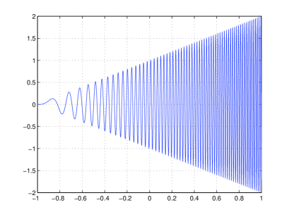
Example 2.6

Highly oscillated and singular functions on $[0,A]$, $\omega=100$, $\epsilon_{QTT}=10^{-6}$,

$$f_{3}(x) =\left\{\begin{array}[]{ll}x+a_{k}\sin(\omega x),&x\in 10\left(\frac{k-1}{p};\frac{k-0.5}{p}\right]\\ 0,&x\in 10\left(\frac{k-0.5}{p};\frac{k}{p}\right]\end{array}\right.$$

$$f_{4}(x) =(x+1)\sin(\omega(x+1)^{2}),\quad x\in[0,1],\quad\mbox{(Fresnel integral)}.$$

where function $f_{3}(x)$, $x\in[0,10]$, $k=1,...,p$, $p=16$, $a_{k}=0.3+0.05(k-1)$, is recognized on three different scales.

The average QTT rank over all mode ranks for the corresponding functional vectors are given in the next table. The maximum rank over all the fibers is nearly the same as the average one.

$N\setminus\overline{r}$	$r_{QTT}(f_{3})$	$r_{QTT}(f_{4})$
$2^{14}$	3.5	6.5
$2^{15}$	3.6	7.0
$2^{16}$	3.6	7.5
$2^{17}$	3.6	7.9

Table 2.1: Average QTT ranks of $N$-vectors generated by $f_{3}$ and $f_{4}$.

Notice that 1D and 2D numerical quadratures based on interpolation by Chebyshev polynomials have been developed [41]. Taking into account that Chebyshev polynomial sampled on Chebyshev grid has exact rank-$2$ QTT representation [67], allows us the efficient numerical integration by Chebyshev interpolation using the QTT approximation.

2.4 Operators in quantized tensor spaces

This section discusses the quantised representation of operators/matrices. The explicit low-rank QTT representations for the wide class of discrete elliptic operators (FEM/FDM matrices) was recently developed in [51, 67, 79, 52, 26].

As the first result is this direction the explicit rank-$3$ QTT representation of ${\Delta}_{1}$ was introduced [51],

$$\Delta_{1} = \begin{bmatrix}I&{J}^{\prime}&J\\ \end{bmatrix}\Join\begin{bmatrix}I&{J}^{\prime}&J\\ &J&\\ &&{J}^{\prime}\\ \end{bmatrix}^{\otimes\left(d-2\right)}\Join\begin{bmatrix}2I-J-{J}^{\prime}\\ -J\\ -{J}^{\prime}\\ \end{bmatrix},$$

with the Pauli matrices

$$I=\left[\begin{array}[]{c c}1&0\\ 0&1\end{array}\right],\quad J=\left[\begin{array}[]{c c}0&1\\ 0&0\end{array}\right].$$

Other results concerning QTT representation of ${\Delta}_{d}$ and its inverse for $d\geq 2$ are collected in Proposition 2.9 below.

The analysis of the low QTT-rank approximations of elliptic operator inverse for $d\geq 2$ is based on certain assumptions on the QTT-rank of the matrix exponential family.

Conjecture 2.7

For any given $\varepsilon>0$, and for fixed $a,b>0$, the family of matrix exponentials, $\{\exp(-t_{k}{{\Delta}_{1}})\}$, $t_{k}>0$, $k=-M,...,M$, allows the QTT $\varepsilon$-approximation with rank-$r_{\Delta}$ being uniformly bounded in the grid size $N$ and in the scaling factors $t_{k}\in[a,b]\subset\mathbb{R}_{>0}$ (see Table 2.2 for numerical justification).

Table 2.2 represents the average QTT-ranks in approximation of certain function related matrices up to fixed tolerance $\varepsilon_{QTT}=10^{-5}$. It includes the important example of matrix exponential (cf. Conjecture 2.7). The matrix $A=diag({f(\|x\|^{2})})$, ($x=(x_{1},x_{2})$, $|x_{i}|\leq 1$) is a diagonal matrix with diagonal entries obtained by sampling a function $f(\|x\|^{2})$ over uniform grid points situated on the diagonal $x_{1}=x_{2}$.

We observe that rank parameters depend very mildly on the grid size.

$N\setminus\overline{r}$	$e^{-\alpha\Delta_{1}},\alpha=0.1/1/10/10^{2}$	$diag({1/\|x\|^{2}})$	$diag({e^{-\|x\|^{2}}})$
$2^{9}$	6.2/6.8/9.7/11.2	5.1	4.0
$2^{10}$	6.3/6.8/9.5/10.8	5.3	4.0
$2^{11}$	6.4/6.8/9.0/10.4	5.5	4.1

Table 2.2: Average QTT ranks of $N\times N$-matrices for large $N=2^{p}$.

We note that the QTT ranks of the matrix $A=diag({f(\|x\|^{2})})$ coincides with those for the generating vector $X$ that follows from the explicit QTT representations (see Def. 2.3). Given vector $X$ and the corresponding rank-${\bf r}_{X}$ QTT-tensor $\textsf{{X}}=\textsf{X}^{(1)}\Join\textsf{X}^{(2)}\Join\cdots\Join\textsf{X}^{(d)}\in\mathbb{X}$, then the QTT representation of the matrix $A=diag(X)$ is given by

$${\bm{\mathcal{A}}}={\cal A}^{(1)}\Join{\cal A}^{(2)}\Join\cdots\Join{\cal A}^{(d)},\quad{\cal A}^{(2)}=diag(\textsf{X}^{(k)}),$$

where $diag(\textsf{X}^{(k)})$ is the matrix diagonalization of the core tensor $\textsf{X}^{(k)}$.

Define the anisotropic $d$-Laplacian

$$\Delta_{d,\alpha}:=\sum\limits_{\ell=1}^{d}\alpha_{\ell}\bigotimes_{k=1}^{d}\Delta_{1}^{\delta_{\ell-k}},\quad\alpha_{\ell}>0,\quad\delta_{m}\quad\mbox{is the Kronecker symbol}.$$ (2.5)

Now we can prove the following Lemma (see [67]).

Lemma 2.8

Under claims of Conjecture 2.7 on the QTT-rank of the univariate matrix exponentials, there exist $C,\beta>0$ independent of $d$, such that for all $M\in\mathbb{N}$,

$$\|{\Delta}_{d,\alpha}^{-1}-{B}_{M}\|\leq Ce^{-\beta\sqrt{M}},\quad\beta>0,$$ (2.6)

where ${B}_{M}$ is defined as

$${B}_{M}:=\sum\limits_{k=-M}^{M}c_{k}\bigotimes_{\ell=1}^{d}\exp(-t_{k}{\alpha_{\ell}{\Delta}_{1}}),\quad t_{k}=e^{k\mathfrak{h}},\quad c_{k}=\mathfrak{h}t_{k},\quad\mathfrak{h}=\pi/\sqrt{M}.$$ (2.7)

Lemma 2.8 implies that the matrix family $\{B_{M}\}$ possesses the low-rank approximation (or preconditioner if $M$ is small) to the anisotropic $d$-Laplacian inverse ${\Delta}_{d,\alpha}^{-1}$, whose ranks scale like $O(\log^{2}\varepsilon)$, where $\varepsilon$ is the error threshold. The constant $\beta>0$ depends logarithmically on the grid size $N$, while $C$ scales linearly in the norm of inverse matrix $\|{\Delta}_{d,\alpha}^{-1}\|$.

The following statement summarizes the previous discussion and the related results in [51].

Proposition 2.9

For $d\geq 2$ the canonical, TT and QTT rank estimates hold:

$$rank_{C}({\Delta}_{d}) =d,\quad rank_{TT}({\Delta}_{d})=2,\quad rank_{QTT}({\Delta}_{d})=4.$$

$$rank_{QTT}({\Delta}_{1}) =3,\quad rank_{QTT}({\Delta}_{1}^{-1})\leq 5.$$

Given $\varepsilon>0$, then for the $\varepsilon$-rank we have

$$rank_{TT}({\Delta}_{d}^{-1}) \leq rank_{C}({\Delta}_{d}^{-1})\leq C|\log\varepsilon|\log N.$$ (2.8)

Moreover, under claims of Conjecture 2.7 there holds

$$rank_{QTT}({\Delta}_{d}^{-1})\leq C|\log\varepsilon|^{2}\log N.$$ (2.9)

In both cases the constant $C$ does not depend on $d$.

The $d$-dimensional FFT over $N^{\otimes d}$ grid can be realized on the rank-$k$ tensor with the linear-logarithmic cost $O(dkN\log_{2}N)$, due to the rank-$1$ factorized representation

$${\cal F}_{N}^{(d)}=(F_{N}^{(1)}\otimes I...\otimes I)(I\otimes F_{N}^{(2)}...\otimes I)...(I\otimes I...\otimes F_{N}^{(d)})\equiv F_{N}^{(1)}\otimes...\otimes F_{N}^{(d)},$$

where $F_{N}^{(\ell)}\in\mathbb{R}^{N\times N}$ represents the univariate FFT matrix along mode $\ell$.

The super-fast Fourier transform of $N$-$d$ tensors can be computed in $\log$-volume complexity, $O(d\log^{2}N)$, by using the QTT approximation as proposed in [24].

Direct convolution transform of $N$-$d$ tensors represented in the canonical/Tucker formats [68, 72], see (2.10), can be implemented in $O(d\log N)$ operations by representing canonical/Tucker vectors by the low-rank QTT tensors (canonical-QTT or Tucker-QTT formats) [60, 61].

The super-fast convolution transform of the complexity $O(d\log^{2}N)$ using the explicit QTT representation of multilevel Toeplitz matrices is developed in [52].

The super-fast QTT wavelet transform of logarithmic complexity by the exact low-rank representation of the wavelet transform matrix was described in [75] (see also [104] for the related discussion).

2.5 Multilinear algebra and tensor-rank truncation

Low-parametric tensor formats provide prerequisites for multidimensional algebraic calculus since the storage complexity of rank-structured tensors scales linearly in dimension $d$. However, the numerical capability of $\varepsilon$-truncated tensor operations is essentially determined by the following issues:

• Understanding of nonlinear tensor approximation in the canonical, Tucker, and MPS/TT formats

• Developments on efficient multilinear algebra and rank optimization algorithms

• Approximation theory for functions and operators in (quantized) tensor spaces

• Construction of stable iterative methods for solving multidimensional PDEs in tensor formats.

It is worth to note that the important multilinear algebraic operations with canonical, Tucker and TT tensors can be implemented with linear complexity scaling in the univariate mode size $N$ and in the dimension $d$ by representing them in terms of tensor operations on rank-$1$ elements.

For example, following [71], for the rank-$R_{1}$ and rank-$R_{2}$ canonical tensors $\textsf{{X}},\textsf{{Y}}\in\mathbb{R}^{\cal I}$, ${\cal I}:=\{1,...,N\}^{d}$, we have

$$\langle\textsf{{X}},\textsf{{Y}}\rangle=\sum\limits_{k=1}^{R_{1}}\sum\limits_{m=1}^{R_{2}}\prod\limits_{\ell=1}^{d}\left\langle\textsf{X}^{(\ell)}_{k},\textsf{Y}^{(\ell)}_{m}\right\rangle,$$

while the Hadamard product is computed by

$$\textsf{{X}}\odot\textsf{{Y}}:=\sum\limits_{k=1}^{R_{1}}\sum\limits_{m=1}^{R_{2}}\left(\textsf{X}^{(1)}_{k}\odot\textsf{Y}^{(1)}_{m}\right)\otimes\ldots\otimes\left(\textsf{X}^{(d)}_{k}\odot\textsf{Y}^{(d)}_{m}\right).$$

We define the discrete convolution product of two convolving tensors [71] by

$$\textsf{{X}}\ast\textsf{{Y}}:=\left[\sum\limits_{{\bf k}\in{\cal I}}{\textsf{X}}_{\bf k}\textsf{Y}_{{\bf j}-{\bf k}}\right]_{{\bf j}\in{\cal J}},\quad{\cal J}:=\{1,...,2N-1\}^{d}.$$

The convolution product of two tensors in the canonical format can be realized in $O(dR_{1}R_{2}N\log N)$ operations [71] relying on the representation

$$\textsf{{X}}\ast\textsf{{Y}}:=\sum\limits_{k=1}^{R_{1}}\sum\limits_{m=1}^{R_{2}}\left(\textsf{X}^{(1)}_{k}\ast\textsf{Y}^{(1)}_{m}\right)\otimes\ldots\otimes\left(\textsf{X}^{(d)}_{k}\ast\textsf{Y}^{(d)}_{m}\right)\in\mathbb{R}^{\cal J},$$ (2.10)

where $\textsf{X}^{(\ell)}_{k}\ast\textsf{Y}^{(\ell)}_{m}\in\mathbb{R}^{2N-1}$ denotes the convolution product of $N$-vectors defined as

$$\textsf{X}^{(\ell)}_{k}\ast\textsf{Y}^{(\ell)}_{m}=\left[\sum\limits_{n=1}^{n}x_{n}y_{j-n}\right]_{j},\quad j=1,...,2N-1.$$

Hence, the one-dimensional convolution can be performed by FFT in $O(N\log N)$ operations. Similarly, the above mentioned tensor operations for Tucker tensors can be reduced to 1D linear algebra [71, 68].

The formatted implementation of the scalar product of TT tensors [98]

$$\langle\textsf{{X}},\textsf{{Y}}\rangle=\langle\textsf{{X}}\odot\textsf{{Y}},{\bf 1}\rangle$$

can be performed by using the Hadamard product in TT format $\textsf{{Z}}=\textsf{{X}}\odot\textsf{{Y}}:\;\textsf{Z}^{(k)}_{i_{k}}=\textsf{X}^{(k)}_{i_{k}}\otimes\textsf{Y}^{(k)}_{i_{k}}.$

Furthermore, the standard multilinear operations like addition, the scalar, Hadamard, contracted and convolution products, etc. in the QTT, QTT-canonical or QTT-Tucker representations can be implemented in $O(d\log N)$ operations and storage costs. This allows fast computations on large spatial grids without practical limitations on $N$, where $N$ is usually associated with the univariate grid size.

Representation of tensors in low separation rank formats is the key point in the design of fast tensor-structured numerical methods for large-scale higher dimensional simulations. In fact, it allows the implementation of basic linear and bilinear algebraic operations on tensors mentioned above with linear complexity in the univariate tensor size (see [68, 69, 51, 56, 24]). However, the bilinear tensor operations normally increase the separation rank of the resultant tensor.

To perform computation over nonlinear set (manifold) of rank-structured tensors ${\cal S}$ (say, the canonical, Tucker, MPS/TT, QTT, and QTT-Tucker formats) with controllable complexity, we need to perform a “projection” of the current iterand in ${\cal S}_{0}\supset{\cal S}$ onto that manifold ${\cal S}$ by using the “formatted“ tensor operations. This action is fulfilled by implementing the tensor truncation operator ${T_{\cal S}}:\mathbb{W}_{{\bf n},d}\to{\cal S}$ defined by

$$\textsf{{A}}_{0}\in{\cal S}_{0}\subset\mathbb{W}_{{\bf n},d}:\quad{T}_{\cal S}\textsf{{A}}_{0}=\operatorname{argmin}_{\textsf{{T}}\in{\cal S}}\|\textsf{{A}}_{0}-\textsf{{T}}\|,$$ (2.11)

that reduces to a challenging nonlinear approximation problem. The replacement of $\textsf{{A}}_{0}$ by its approximation in ${\cal S}$ is called the tensor truncation to ${\cal S}$ and denoted by ${T}_{\cal S}\textsf{{A}}_{0}$. In practice, the computation of the minimizer ${T}_{\cal S}\textsf{{A}}_{0}$ can be performed only approximately. The set ${\cal S}$ of rank-structured tensors can be chosen adaptively in order to control the approximation error $\varepsilon>0$,

$$\|\textsf{{A}}_{0}-{T}_{\cal S}\textsf{{A}}_{0}\|\leq\varepsilon.$$

In the case of Tucker, TT/QTT and QTT-Tucker formats the quasi-optimal approximation can be computed by conventional QR/SVD algorithm [83, 102, 37, 23], also known in the physical literature as the Schmidt decomposition. In particular, the Tucker tensors can be approximated by the so-called higher order SVD (HOSVD), [22]. Robust SVD-based algorithms are applicable since the Tucker and TT ranks can be controlled by a certain matrix rank. Indeed, for MPS/TT format we have the equivalent definition in terms of the TT-unfolding matrix, $TT[{\bf r}]:=\{\textsf{{A}}\in\mathbb{V}_{\bf n}:\mathop{\mathrm{rank}}\nolimits A_{[p]}\leq r_{p}$, p=1,…,d-1 }, where the TT-unfolding matrix $A_{[p]}$ is defined by

$$A_{[p]}:=\textsf{{A}}(\underbrace{{j_{1}\>j_{2}\>\ldots j_{p}}}_{\mbox{column ind.}};\underbrace{{\color[rgb]{0,0,1}\definecolor[named]{pgfstrokecolor}{rgb}{0,0,1}j_{p+1}\ldots j_{d}}}_{\mbox{row ind.}}).$$

For the Tucker format we have the alternative definition ${\cal T}[{\bf r}]:=\{{\textsf{{A}}}\in\mathbb{V}_{\bf n}:\mbox{rank}\,A_{(p)}\leq r_{p},p=1,...,d\}$, where the Tucker unfolding matrix $A_{(p)}$ is defined by

$$A_{(p)}:=\textsf{{A}}(\underbrace{{\color[rgb]{0,0,1}\definecolor[named]{pgfstrokecolor}{rgb}{0,0,1}j_{1}\>j_{2}\>\ldots j_{p-1}}}_{\mbox{row ind.}};\underbrace{{j_{p}}}_{\mbox{column ind.}};\underbrace{{\color[rgb]{0,0,1}\definecolor[named]{pgfstrokecolor}{rgb}{0,0,1}j_{p+1}\ldots j_{d}}}_{\mbox{row ind.}}).$$

In turn, the canonical and TC ranks can not be identified with certain matrix ranks that may result in instabilities of approximation schemes. Approximation in the $R$-term canonical format is considered as a subtle problem that cannot in general be solved by a stable algorithms in polynomial cost. One of the reasons is that the set of canonical tensors with rank $\leq R$ is not closed as shown by the following example.

Example 2.10

The tensor F, with $rank_{Can}(\textsf{{F}})={d}$, generated by sampling of the function $f(x)=x_{1}+...+x_{d}$ on a tensor grid can be approximated with arbitrary precision by rank-$2$ elements

$$\textsf{{F}}=\lim_{\varepsilon\to 0}\frac{{\bigotimes}_{\ell=1}^{d}(1+\varepsilon X_{\ell})-1}{\varepsilon}.$$

However, for some classes of functions and operators the robust analytic methods based on $R$-term explicit $\operatorname{sinc}$-quadrature approximations can be successfully applied (see [69] and references therein).

Notice that the so-called reduced HOSVD (RHOSVD) method introduced in [72] provides robust rank reduction for the canonical tensors with large initial rank. This is a two-step method which, first, reduces the canonical tensor to low-rank Tucker form by SVD-based low-rank approximation of the factor matrices, and then applies the ALS type rank reduction iteration to the small-size Tucker core to represent it in canonical format. The RHOSVD method was successfully applied in electronic structure calculations [72, 55, 56, 73].

3 Tensor numerical methods for $d$-dimensional PDEs

In this section, we discuss the benefits of tensor numerical methods (TNM) in two important applications: the nonlinear Hartree-Fock (HF) equation in electronic structure calculations (§3.1) and the real-time parabolic equations in many-particle dynamics (§3.2).

The numerical challenge in the HF calculations is due to the presence of large number of complicated convolution-type integrals in $\mathbb{R}^{3}$, multiply recomputed within the iterations on nonlinearity, as well as hard complexity scaling of the traditional methods with respect to the size of a molecular system (see for example [89, 108] and references therein). At this point the beneficial features of tensor computations has been successfully realized in the form of fast grid-based black-box HF-solver that manifests linear complexity in the univariate grid size [72, 73, 56, 57, 61]. The latter can be reduced to the logarithmic scale by implementation in quantized tensor spaces [60]. Further steps toward TNMs for post Hartree-Fock calculations [59], and for solving the Hartree-Fock problem for large lattice-structured and periodic systems [62, 63] are the subject of current research.

The real space numerical methods combined with FEM approximations have become attractive in electronic structure calculations as the possible alternative to the traditional approaches (see [87, 47, 74, 16, 34, 107] and references therein).

For a class of multi-dimensional parabolic problems including, in particular, the molecular Schrödinger, the Fokker-Planck and master equations, the computational challenges arise due to the curse of dimensionality. We discuss the main issues which allow to understand how the $d$-dimensional dynamics can be simulated in quantized tensor spaces with the linear complexity in $d$ and in log-log complexity in the mesh size for simultaneous space-time discretization. Further details can found in [69, 25, 36, 26]. Exposition of tensor methods based on the Dirack-Frenkel variational principle implemented on the Tucker and MPS/TT tensor manifolds can be found in [91, 92, 101] and references therein.

Recently, the TNM were shown to be efficient for solving parameter dependent PDEs in the case of high dimensional parametric space [81, 76, 13, 27].

Another popular topic in numerical analysis of multidimensional PDEs is concerned with the so-called greedy methods and their applications [90, 9, 19, 33], which became attractive since the simplicity of greedy algorithms: the main step usually includes either rank-$1$ corrections low-rank tensors in other formats commonly used in practice. Due to the page limits, these topics will not be further addressed in this paper.

3.1 Hartree-Fock equation in electronic structure calculations

3.1.1 Problem setting

The HF equation for determination of the ground state energy of a molecular system consisting of $M$ nuclei and $N_{orb}$ electrons (closed shell case) is given by the following nonlinear eigenvalue problem in $H^{1}(\mathbb{R}^{3})$ [89],

$$({\cal F}\phi_{i})({x})=\lambda_{i}\,\phi_{i}({{x}}),\quad\int_{\mathbb{R}^{3}}\phi_{i}({x})\phi_{j}({x})\,\mathrm{d}{x}=\delta_{ij},\;i,j=1,...,N_{orb},$$ (3.1)

where the non-linear integral-differential Fock operator ${\cal F}$ is given by

$${\cal F}:=-\frac{1}{2}\Delta-V_{c}+V_{H}+{\cal V}_{E},\quad V_{c}=\sum_{\nu=1}^{M}\frac{Z_{\nu}}{\|{x}-{A}_{\nu}\|},$$ (3.2)

with the Hartree potential, $V_{H}(x)$, and the nonlocal exchange operator, ${\cal V}_{E}$, defined by

$$V_{H}({x}):=\int_{\mathbb{R}^{3}}\frac{\tau({y},{y})}{\|{x}-{y}\|}\,\mathrm{d}\textbf{y},\quad\mbox{and}\quad{\cal V}_{E}\phi:=-\frac{1}{2}\int_{\mathbb{R}^{3}}\frac{\tau({x},{y})}{\|{x}-{y}\|}\phi({y})\,\mathrm{d}{y},$$

respectively. Here, $1/{\|\cdot\|}:\mathbb{R}^{3}\to\mathbb{R}$ corresponds to the Newton potential, and $Z_{\nu}\in\mathbb{R}_{+}$, ${A}_{\nu}\in\mathbb{R}^{3}$ ($\nu=1,...,M$) specify charges and positions of $M$ nuclei. The electron density matrix $\tau:\mathbb{R}^{3}\times\mathbb{R}^{3}\to\mathbb{R}$, is given by $\tau({x},{y})=2\sum_{i=1}^{N_{orb}}\phi_{i}({x})\phi_{i}^{*}({y}),$ specifying the electron density $\rho(x)=\tau({x},{x})$.

Notice that the Hartree-Fock equation is a nonlinear eigenvalue problem in a sense, that one should solve it when the nonlinear part $V_{H}+{\cal V}_{E}$ of the governing operator depending on the eigenvectors is unknown. This dependence is expressed by the 3D convolution transform with the Newton convolving kernel, while the electron density $\rho(x)$ contains multiple strong singularities corresponding to each nuclei location. Therefore solution of the HF equation requires iterative solvers, with multiply repeated recalculation of these convolution integrals.

Usually, the Hartree-Fock equation is approximated by the standard Galerkin projection of the initial problem (3.1) posed in $H^{1}(\mathbb{R}^{3})$ (see [89] for more details). For a given finite Galerkin basis set $\{g_{\mu}\}_{1\leq\mu\leq N_{b}}$, $g_{\mu}\in H^{1}(\mathbb{R}^{3})$, the molecular orbitals $\phi_{i}$ are expanded (approximately) by

$$\phi_{i}=\sum\limits_{\mu=1}^{N_{b}}C_{\mu i}g_{\mu},\quad i=1,...,N_{orb},$$ (3.3)

yielding the Galerkin system of nonlinear equations for the coefficients matrix $C=\{c_{\mu i}\}\in\mathbb{R}^{N_{b}\times N_{orb}}$, concatenating the eigenvectors $C_{i}\in\mathbb{R}^{N_{b}}$ (and the density matrix $D=2CC^{\ast}\in\mathbb{R}^{N_{b}\times N_{b}}$)

$$F(D)C=SC\Lambda,\quad\Lambda=diag(\lambda_{1},...,\lambda_{N_{b}}),\quad C^{T}SC=I_{N_{b}},$$ (3.4)

where $S$ is the overlap (stiffness) matrix for $\{g_{\mu}\}_{1\leq\mu\leq N_{b}}$, and the Fock matrix

$$F(D)=H+J(D)+K(D),$$ (3.5)

is a sum of the stiffness matrix $H=\{h_{\mu\nu}\}$ of the core Hamiltonian ${\cal H}=-\frac{1}{2}\Delta+V_{c}$ (the single-electron integrals),

$$h_{\mu\nu}=\frac{1}{2}\int_{\mathbb{R}^{3}}\nabla g_{\mu}\cdot\nabla g_{\nu}dx+\int_{\mathbb{R}^{3}}V_{c}(x)g_{\mu}g_{\nu}dx,\quad 1\leq\mu,\nu\leq N_{b},$$

and the two nonlinear terms $J(D)+K(D)$, representing the Galerkin approximation to the Hartree and exchange operators. This is the main computational task, which is traditionally calculated by using the two-electron integrals tensor $\textsf{{B}}=[b_{\mu\nu\kappa\lambda}]$, defined as follows: Given the finite basis set $\{g_{\mu}\}_{1\leq\mu\leq N_{b}}$, $g_{\mu}\in H^{1}(\mathbb{R}^{3})$, the associated fourth order two-electron integrals (TEI) tensor, $\textsf{{B}}=[b_{\mu\nu\kappa\lambda}]$, is defined entrywise by

$$b_{\mu\nu\kappa\lambda}=\int_{\mathbb{R}^{3}}\int_{\mathbb{R}^{3}}\frac{g_{\mu}(x)g_{\nu}(x)g_{\kappa}(y)g_{\lambda}(y)}{\|x-y\|}dxdy,\quad\mu,\nu,\kappa,\lambda\in\{1,...,N_{b}\}.$$ (3.6)

In the straightforward implementation based on the analytically precomputed integrals, the computational and storage complexity for the TEI tensor is of order $O(N_{b}^{4})$, or even $O(N_{b}^{5})$, that becomes non-tractable already for $N_{b}$ of order of several hundred.

Given TEI tensor, the $N_{b}\times N_{b}$ matrices $J(D)$ and $K(D)$ can be represented by

$$J(D)_{\mu\nu}=\sum\limits_{\kappa,\lambda=1}^{N_{b}}b_{\mu\nu,\kappa\lambda}D_{\kappa\lambda},\quad K(D)_{\mu\nu}=-\frac{1}{2}\sum\limits_{\kappa,\lambda=1}^{N_{b}}b_{\mu\lambda,\nu\kappa}D_{\kappa\lambda},$$ (3.7)

with the low-rank symmetric density matrix, $D=2CC^{T}\in\mathbb{R}^{N_{b}\times N_{b}}$, such that $rank(D)=N_{orb}\ll N_{b}.$ Equations (3.7) can be rewritten in terms of the TEI matrix $B=[b_{\mu\nu,\kappa\lambda}]\in\mathbb{R}^{N_{b}^{2}\times N_{b}^{2}}$.

The total energy is computed as

$$E_{HF}=2\sum\limits_{i=1}^{N_{orb}}\lambda_{i}-\sum\limits_{i=1}^{N_{orb}}\left(\widetilde{J}_{i}-\widetilde{K}_{i}\right),$$

where $\widetilde{J}_{i}=(\phi_{i},V_{H}\phi_{i})_{L^{2}}=\langle C_{i},JC_{i}\rangle$ and $\widetilde{K}_{i}=(\phi_{i},K\phi_{i})_{L^{2}}=\langle C_{i},KC_{i}\rangle$, $i=1,...,N_{orb}$, are the Coulomb and exchange integrals in the basis of orbitals $\phi_{i}$. The resulting ground state energy of a molecule, $E_{0}$, for the given geometry of nuclei, includes the nuclei repulsion energy $E_{nuc}$,

$$E_{0}=E_{HF}+E_{nuc},\quad\mbox{ where }\quad E_{nuc}=\sum^{M}_{k=1}\sum^{M}_{m<k}\frac{Z_{k}Z_{m}}{\|x_{k}-x_{m}\|}.$$ (3.8)

The standard quantum chemical implementations are based on the analytically precomputed set of the two-electron integrals (3.6) in a naturally separable Gaussian basis with the computational and storage complexity for the TEI tensor of order $O(N_{b}^{4})$, or even $O(N_{b}^{5})$, that becomes non-tractable already for $N_{b}$ of order of several hundred.

3.1.2 Grid-based tensor numerical methods

The tensor-structured numerical methods, both the name and the concept, appeared during the work on the 3D grid-based tensor approach to the solution of the Hartree-Fock equation. They lead to “black-box” numerical treatment of the Hartree-Fock problem based on the low-rank representation of the basis functions in a volume box, using the $n\times n\times n$ $3D$ Cartesian grid positioned arbitrarily with respect to the atomic centers [73, 58, 61, 56]. In 2008 [72, 55] it was shown that within the tensor-structured paradigm the core Hamiltonian and the $3D$ convolutions with the Newton kernel, involved in the Coulomb and exchange operators, can calculated in $1D$ complexity by the rank-structured tensor operations reduced to $1D$ convolutions, Hadamard and scalar products [68, 72, 57]. Due to elimination of the analytical integrability requirements it gives a choice to use rather general physically relevant basis sets represented on the grid. High accuracy is achieved due to grid-sizes up to the order of $n\simeq 10^{6}$, yielding a volume box of size $n^{3}\simeq 10^{18}$. It corresponds to mesh resolution up to $h=10^{-5}$ $\stackrel{{\scriptstyle\circ}}{{A}}$ (close to sizes of atomic radii) in the volume box with the equal sizes of $20\,\stackrel{{\scriptstyle\circ}}{{A}}$ for each spatial variable. Matlab on a Sun station is used for all algorithms, without parallelizations and supercomputing.

Chronologically, two different approaches have been developed for the 3D grid-based tensor-structured solution of the HF equation. Both use the rank-structured calculation of the core Hamiltonian [58, 57] for a given grid-based basis set.

• The tensor solver I does not use the two-electron integrals. Instead, the Coulomb and exchange operators are recomputed “on the fly” using the refined 3D grids and rank-structured (1D) operations. [55, 73, 56]. This approach has low storage demand, but might be time consuming. It can be applicable to the Kohn-Sham type models.

• The “black-box“ solver II based on calculation of the TEI matrix $B$ by the truncated Cholesky decomposition and the redundancy-free factorization by the algebraically reduced product basis yielding the reduced storage consumption $O(N_{b}^{3})$ [59, 60, 57]. Its performance in time and accuracy is compatible with the benchmark packages in quantum chemistry based on analytical pre-calculation of involved multidimensional integrals.

In the following, we briefly discuss the tensor algorithm for computation of TEIs used in the solver II. We suppose that all basis functions $\{g_{\mu}\}_{1\leq\mu\leq N_{b}}$, are supported by the finite volume box $\Omega=[-b,b]^{3}\in\mathbb{R}^{3}$, and assume, for ease of presentation, that $rank(g_{\mu})=1$. Introducing the $n\times n\times n$ Cartesian grid over $\Omega$ and using the standard collocation discretization in the volume by piecewise constant basis functions, we define a grid-based tensor representation of the initial basis set $g_{\mu}(x)\in\mathbb{R}^{3}$, $\mu=1,\ldots N_{b}$,

$$g_{\mu}(x)=g_{\mu}^{(1)}(x_{1})g_{\mu}^{(2)}(x_{2})g_{\mu}^{(3)}(x_{3})\approx{\bf G}_{\mu}=G_{\mu}^{(1)}\otimes G_{\mu}^{(2)}\otimes G_{\mu}^{(3)}\in\mathbb{R}^{n\times n\times n}.$$

Define the respective product-basis tensor

$$\textsf{{G}}=[{\bf G}_{\mu\nu}]\in\mathbb{R}^{N_{b}\times N_{b}\times n^{\otimes 3}}\quad\mbox{with}\quad{\bf G}_{\mu\nu}={\bf G}_{\mu}\odot{\bf G}_{\nu}\in\mathbb{R}^{n^{\otimes 3}},$$

where $\mu,\nu\in\{1,...,N_{b}\}$, then both the TEI tensor and matrix are represented by tensor operations,

$$\textsf{{B}}=\textsf{{G}}\times_{n^{\otimes 3}}\textsf{{P}}\ast_{n^{\otimes 3}}\textsf{{G}},\quad b_{\mu\nu,\kappa\lambda}=\left\langle{\bf G}_{\mu\nu},\textsf{{P}}\ast{\bf G}_{\kappa\lambda}\right\rangle_{n^{\otimes 3}}.$$ (3.9)

Here the rank-$R_{\cal N}$ canonical tensor $\textsf{{P}}=\sum\limits_{k=1}^{R_{\cal N}}{P}^{(1)}_{k}\otimes{P}^{(2)}_{k}\otimes{P}^{(3)}_{k}\in\mathbb{R}^{n^{\otimes 3}}$ approximates the Newton potential $\frac{1}{\|x\|}$ (see [14, 72] for more details), $\ast$ stands for the 3D tensor convolution, and $\odot$ denotes the Hadamard product of tensors.

Though tensor methods reduce the multidimensional integration to 1D complexity operations, the direct tensor-structured evaluation of (3.9) needs a storage size of at least, $O(R_{\cal N}N_{b}^{2}n)$, which can be prohibitive for large $N_{b}\sim 10^{2}$ and $n\approx 10^{5}$. We apply the RHOSVD-type factorization [72] to the $4$th order tensor G by approximating its site matrices, $G^{(\ell)}\in\mathbb{R}^{n\times N_{b}^{2}}$, ($\ell=1,2,3$) in a “squeezed” factorized form, $G^{(\ell)}\cong U^{(\ell)}{V^{(\ell)}}^{T}$, according to the chosen $\varepsilon$-truncation. This step can be implemented by the truncated SVD in combination with incomplete truncated Cholesky decomposition.

This provides the construction of dominating subspaces in the $x$-, $y$- and $z$- components in the product basis set defined by an $n\times R_{\ell}$ matrix $U^{(\ell)}$ (left orthogonal basis) and $N_{b}^{2}\times R_{\ell}$ matrix $V^{(\ell)}$ (right basis). Then for the TEI matrix $B\in\mathbb{R}^{N_{b}^{2}\times N_{b}^{2}}$, we obtain a factorization [61, 59],

$$B\cong B_{\varepsilon}:=\sum\limits^{R_{\cal N}}_{k=1}\odot^{3}_{\ell=1}V^{(\ell)}M_{k}^{(\ell)}{V^{(\ell)}}^{T},$$ (3.10)

where $V^{(\ell)}$ is the corresponding right redundancy-free basis, $\odot$ denotes the point-wise (Hadamard) product of matrices, and

$$M_{k}^{(\ell)}={U^{(\ell)}}^{T}(P_{k}^{(\ell)}\ast_{n}U^{(\ell)})\in\mathbb{R}^{R_{\ell}\times R_{\ell}},\quad k=1,...,R_{\cal N}.$$ (3.11)

Ultimately, the TEI matrix $B$ is approximated in a form of the truncated Cholesky factorization, $B\approx LL^{T}$, $L\in\mathbb{R}^{N_{b}^{2}\times R_{B}}$ ($R_{B}=O(N_{b})$), such that the required columns of $B$ are easily computed by using (3.10).

Vectorizing matrices $\overline{J}=vec(J(D))$, $\overline{K}=vec(K(D))$, $\overline{D}=vec(D)$, we arrive at the simple matrix representations,

$$\overline{J}=B\overline{D}\approx L(L^{T}\overline{D}),\quad vec(K)=\overline{K}=\widetilde{B}\overline{D},$$ (3.12)

where $\widetilde{B}=mat(\widetilde{\textsf{{B}}})$ is the matrix unfolding of the permuted tensor $\widetilde{\textsf{{B}}}=[\widetilde{b}_{\mu\nu\kappa\lambda}]$ such that $\widetilde{b}_{\mu\nu\kappa\lambda}={b}_{\mu\kappa\nu\lambda}$.

The nonlinear eigenvalue problem (3.4) is solved by the commonly used DIIS self-consistent iteration which requires the update of both Hartree and exchange operators at each iterative step.

3.1.3 Numerical illustrations

Figure 3.1, left, illustrates the convergence history for self-consistent iterations by tensor solver II compared with the output of a standard quantum chemical package MOLPRO based on analytical calculations [122] for the Glycine amino acid, $C_{2}H_{5}NO_{2}$. The basis set cc-pVDZ of 170 Gaussians is used for both analytical and 3D grid-based calculations. Here TEI is calculated on the grids $n^{3}=131072^{3}$. For this iteration the core Hamiltonian is taken from MOLPRO. Time for one iteration is about $6$ seconds in Matlab.

Figure 3.1: Left: iterations history for Glycine molecule with TEI calculated on the grids $n^{3}=131072^{3}$. Middle: convergence in energy. Right: a zoom for energy difference at last iteration.

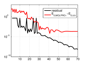
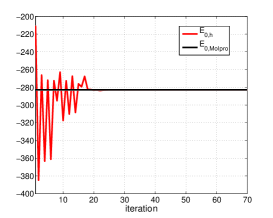
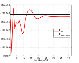
We observe, that though the residual displays good convergence (in max-norm), the error with respect to analytical calculations stagnates at $2\cdot 10^{-4}$ (relative error $<7\cdot 10^{-7}$). Figure 3.1 middle, shows the convergence in ground state energy $E_{0,it,h}$ while the right figure displays the zoomed difference of ground state energy for last iterations. Here the energy $E_{0,it,h}$ is computed by (3.8) at each iteration step $it$ representing the convergence history. The stagnation in the energy on lower than MOLPRO level (relative error $7\cdot 10^{-7}$) may indicate the actual accuracy in computation of 3D convolution integrals in that code, and, beside, some possible instabilities of the grid-based algorithms applied on huge spatial grids ($n^{3}=131072^{3}$). This topic needs further analysis to be conducted elsewhere.

Figure 3.2: Left: the error in density matrix resulting from calculations of TEI on a grid of size $n^{3}=65536^{3}$. Middle: the same error for the grid size $n^{3}=131072^{3}$. Right: the error in density matrix for Alanine amino acid, TEI computed with $n^{3}=32768^{3}$.

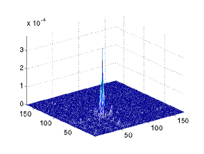
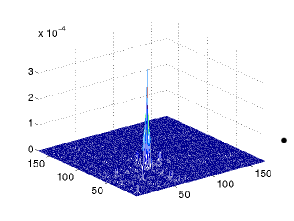
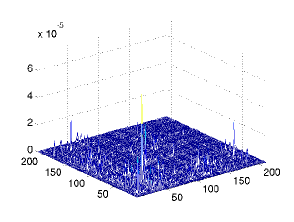
Figures 3.2 (left, middle) show the absolute error (scaled by factor $10^{-4}-10^{-5}$), with respect to MOLPRO output, of the tensor calculation of the density matrix for Glycine amino acid using TEI computed on the grids $n^{3}=65536^{3}$ (left) and $n^{3}=131072^{3}$ (middle). Figure 3.2 (right) shows the error of tensor calculations for Alanine amino acid, $C_{3}H_{7}NO_{2}$, using TEI computed on the grid $n^{3}=32768^{3}$, with $N_{b}^{2}=211^{2}$ basis functions.

The dominating part in the above tensor calculus resulted by rather large mode size $n$, can be reduced to the logarithmic scale in $\log n$ by applying the QTT approximation. Numerical illustrations on the QTT approximation of functions and operators arising in the solution of Hartree-Fock equation are given in Table 3.1.

$n^{3}$	$2^{14\cdot 3}$	$2^{15\cdot 3}$	$2^{16\cdot 3}$	$2^{17\cdot 3}$
$1/\|x\|$	3.15	3.13	3.13	3.11
$g_{\mu}g_{\nu}$	3.77	3.78	3.76	3.76

Table 3.1: Average QTT-ranks for canonical vectors of the tensor P, and for the product basis $\{g_{\mu}g_{\nu}\}$ designed for CH₄ molecule.

It indicates the low QTT-rank approximability of (a) the canonical vectors in low-rank decomposition P of the Newton kernel $1/\|x\|$, in $\mathbb{R}^{3}$, see [72], (b) the product basis set designed for CH₄ molecule, both discretized over large $n\times n\times n$ spatial grids. In all cases the QTT approximation accuracy $\varepsilon=10^{-6}$ is achieved. We observe that QTT-ranks of canonical vectors for both the Newton potential and the product basis remain practically constant in $n$, ensuring $O(\log\varepsilon^{-1}\log n)$ complexity scaling.

These results show that the grid-based tensor-structured Hartree-Fock solver II provides the accuracy and computation time compatible with the analytical calculations from MOLPRO. More numerical results, including the complete grid-based calculations with the grid-based core Hamiltonian and their comparison with MOLPRO are given in [57]. The Laplacian in core Hamiltonian is calculated on large 3D grids by using the QTT format.

We summarize that tensor numerical methods described above are implemented in the Matlab program package Tensor-based Electronic Structure Calculation (TESC) by V. Khoromskaia and B. Khoromskij. TESC package allows the efficient grid-based solution of the 3D nonlinear Hartree-Fock equation discretized in a general set of basis functions characterized by the existence of low-rank separable representation. All 3D and 6D integrals involved are approximated on large $n\times n\times n$ grids and computed by the black-box algorithms in the 1D complexity, $O(n)$, or even in $O(\log n)$ operations, which allows us the high resolution with the grid size up to $n=10^{6}$.

Further work should be focused, in particular, on the developments of the general type basis functions. Now preliminary results are obtained for products of Gaussians with the plane waves.

3.1.4 Tensor method for fast lattice summation

The recent progress in tensor numerical methods for Hartree-Fock calculations is concerned with the generalization of the above mentioned approach to the case of large lattice structured and periodic systems [62, 63] arising in the modeling of cristalline, metallic and polymer type compounds.

To fix the idea, we consider the electrostatic potential $V_{c}(x)$ in (3.2) in the simplest case $M=1$. Defined the scaled unit cell $\Omega_{0}=[-b/2,b/2]^{3}$, of size $b\times b\times b$. We consider a sum of interaction potentials in a symmetric box

$$\Omega_{L}=B\times B\times B,\quad\mbox{with}\quad B=\frac{b}{2}[-L,L],\quad L\in\mathbb{N},$$

consisting of a union of $L\times L\times L$ unit cells $\Omega_{\bf k}$, obtained from $\Omega_{0}$ by a shift specified by the lattice vector $b{\bf k}$, where ${\bf k}=(k_{1},k_{2},k_{3})\in\mathbb{Z}^{3}$, $-(L-1)/2\leq k_{\ell}\leq(L-1)/2$, ($\ell=1,2,3$). Here $L=1$ corresponds to a system in the unit cell. Recall that $b=nh$, where $h>0$ is the mesh size that is the same for all spatial variables, and $n$ is the number of grid points for each variable. We also define the accompanying domain $\widetilde{\Omega}_{L}$ obtained by scaling of ${\Omega}_{L}$ with the factor of $2$, $\widetilde{\Omega}_{L}=2{\Omega}_{L}$, and introduce the respective rank-$R$ master tensor $\widetilde{\bf P}=\sum\limits_{q=1}^{R}\widetilde{P}^{(1)}_{q}\otimes\widetilde{P}^{(2)}_{q}\otimes\widetilde{P}^{(3)}_{q}$, approximating $\frac{1}{\|{x}\|}$ in $\widetilde{\Omega}_{L}$ on tensor grid with mesh size $h$.

In the case of extended system in a box the summation problem for the total potential $V_{c_{L}}$ is formulated in the domain $\Omega_{L}=\bigcup_{k_{1},k_{2},k_{3}=-(L-1)/2}^{(L-1)/2}\Omega_{\bf k}$ as well as in the accompanying domain. On each $\Omega_{\bf k}\subset\Omega_{L}$, the target potential $v_{\bf k}(x)=(V_{c_{L}})_{|\Omega_{\bf k}}$, is obtained by summation over all unit cells in $\Omega_{L}$,

$$v_{\bf k}(x)=\sum\limits_{k_{1},k_{2},k_{3}=-(L-1)/2}^{(L-1)/2}\frac{Z_{0}}{\|{x}-b{\bf k}\|},\quad x\in\Omega_{\bf k}.$$

This calculation is performed at each of $L^{3}$ elementary cells $\Omega_{\bf k}\subset\Omega_{L}$ simultaneously, which is implemented by the assembled tensor summation method described in [62]. The resultant lattice sum is presented by the canonical rank-$R$ tensor ${\bf P}_{c_{L}}\in\mathbb{R}^{nL\times nL\times nL}$,

$${\bf P}_{c_{L}}=Z_{0}\sum\limits_{q=1}^{R}(\sum\limits_{k_{1}=-(L-1)/2}^{(L-1)/2}{\cal W}_{{k_{1}}}\widetilde{P}^{(1)}_{q})\otimes(\sum\limits_{k_{2}=-(L-1)/2}^{(L-1)/2}{\cal W}_{{k_{2}}}\widetilde{P}^{(2)}_{q})\otimes(\sum\limits_{k_{3}=-(L-1)/2}^{(L-1)/2}{\cal W}_{{k_{3}}}\widetilde{P}^{(3)}_{q}),$$ (3.13)

where ${\cal W}_{{k_{\ell}}}$ is the shift-and-windowing transform along the ${\bf k}$-grid. The numerical cost and storage size are bounded by $O(RLN_{L})$, and $O(RN_{L})$, respectively (see [62], Theorem 3.1), where $N_{L}=nL$, and $n$ is the grid size in the unit cell.

The lattice sum in (3.13) converges only conditionally as $L\to\infty$. This aspect was addressed in [62].

Figure 3.3: Canonical vectors in the assembled $10\times 4\times 6$ lattice sum.

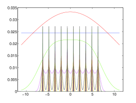
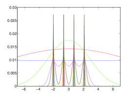
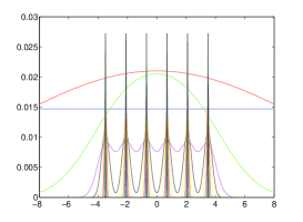
Figure 3.3 demonstrates the canonical vectors for assembled tensor sum corresponding to $10\times 4\times 6$ lattice.

3.2 Real-time dynamics by parabolic equations

3.2.1 General introduction

Let $\mathbb{W}$ be a complex Hilbert space and ${\cal H}$ be a self-adjoint positive definite operator with the domain $D({\cal H})$ and the spectrum $\Sigma({\cal H})\in[\lambda_{0},\infty),\lambda_{0}>0$. Given $\sigma\in\{-1,i\}$, we consider the following initial value problem

$$\frac{\partial\psi}{\partial t}=\sigma{\cal H}\psi(t),\quad\psi(0)=\psi_{0}\in D({\cal H})\subset\mathbb{W}.$$ (3.14)

The solution of (3.14) is represented by using operator exponential, $\psi(t)=e^{\sigma{\cal H}t}\psi_{0},$ however, in general, the solution operator of this parabolic problem, $S(t)=e^{\sigma{\cal H}t}$, does not allow the accurate low-rank tensor approximation.

In quantum mechanics, equation like (3.14) may represent the molecular or electronic Schrödinger equation in $d$ dimensions that describes how the quantum state of a physical system evolves in time. In this case the many particle Hamiltonian ${\cal H}$ is given by a sum of $d-$dimensional Laplacian and certain interaction potential, [91],

$$i\frac{\partial\psi}{\partial t}={\cal H}\psi=(-\frac{1}{2}\Delta_{d}+V)\psi,\quad\psi(x,0)=\psi_{0}(x),\quad x\in\mathbb{R}^{d},$$

where $V:\mathbb{R}^{d}\to\mathbb{R}$ is (given) approximation to the potential energy surface (PES).

The interesting example of the real-time dynamics is given by the Fokker-Planck equation, which is usually high-dimensional. It models the joint probability density distribution of noisy dynamical system configurations (e.g. positions of particles). The initial (stochastic) system of ODEs reads

$$\dfrac{dx}{dt}=-A(x)+G\eta\in\mathbb{R}^{d},$$

where the noise satisfies $<\eta>=0$, and $<\eta_{i}\eta_{j}>=\delta_{ij}$. The probability to find configurations in some volume $x^{*}+dx$ is written as follows,

$$P\left(x\in\mathbb{B}_{|dx|}(x^{*})\right)=\psi(x^{*})dx,$$

and the deterministic real-time parabolic PDE on the probability density, called the Fokker-Planck equation, reads as

$$\psi(0)=\psi_{0}:\quad\dfrac{\partial\psi}{\partial t}=\dfrac{\partial}{\partial x}\cdot\left(A(x)\psi\right)+\dfrac{1}{2}\dfrac{\partial}{\partial x}\cdot\left(D\dfrac{\partial\psi}{\partial x}\right),\quad\mbox{where}\quad D=GG^{T}.$$

Here $\psi:\mathbb{R}^{d}\rightarrow\mathbb{R}$, and ${\bf v}:\mathbb{R}^{d}\rightarrow\mathbb{R}^{d}$ is a given velocity field. In many cases the computation of stationary solution $\psi(t)\to\psi_{\ast}:A\psi_{\ast}=0$, is the main target. We refer to [25] for detailed discussion and numerical tests.

In Section 3.2.3 we discuss in more detail the tensor numerical scheme for the solution of chemical master equation. This model describes the dynamics of joint probability density ${\cal P}({\bf x},t)$,

$${\cal P}({\bf x},0)={\cal P}_{0},\quad\frac{d{\cal P}({\bf x},t)}{dt}={\bf A}{\cal P}({\bf x},t),\quad{\bf x}\in\mathbb{R}^{n_{1}\times...\times n_{d}},$$ (3.15)

where ${\cal P}({\bf x},t)$ is the joint probability of the numbers of molecules of species $S_{1},...,S_{d}$, reacting in $M$ channels, to take particular values $x_{1},...,x_{d}$ at time $t$.

3.2.2 Rank bounds for Cayley transform in space-time tensor approximation

In [36] the QTT-Cayley transform was proposed to compute dynamics and spectrum of high-dimensional Hamiltonians with the focus on complex-time dynamics. Here, using the similar techniques, we analyze in more detail the case of real-time dynamics, i.e. $\sigma=-1$ in (3.14), already sketched in [36]. For the ease of presentation, we further assume that the self-adjoint Hamiltonian operator ${\cal H}$ has the complete eigenbasis, $\mathbb{W}=\operatorname{span}\{\phi_{n}\}_{n=0}^{\infty}$, with the real eigenvalues $0<\lambda_{0}\leq\lambda_{1}\leq...$. An extension to the more general class of convection-diffusion operators as in (3.2.1) is possible and it will be addressed elsewhere.

The idea on separation of the time and space variables via Cayley transform is based on the series expansion for the solution operator

$$e^{-{\cal H}t}=({\cal H}+I)^{-1}\underset{p=0}{\overset{\infty}{\sum}}L_{p}(t){\cal C}^{p}({\cal H}),$$ (3.16)

where ${\cal C}={\cal C}({\cal H})={\cal H}({\cal H}+I)^{-1}$ is the Cayley transform of the operator ${\cal H}$, and $L_{p}(t)=L_{p}^{(0)}(t)$ is the Laguerre polynomial of degree $p$ [113, 10]. Expansion (3.16) applies (convergence in $\mathbb{W}$ norm) to every initial vector $\psi_{0}\in D({\cal H})$, i.e.,

$$\psi_{0}=\sum\limits_{k=0}^{\infty}a_{k}\phi_{k},\quad\mbox{such that}\quad\sum\limits_{k=0}^{\infty}|a_{k}|^{2}\lambda_{k}^{2}<\infty.$$ (3.17)

Separation of the time variable $t$ from the spatial part of the solution is based on the observation that the solution of our initial value problem subject (3.17) can be represented as

$$\psi(t)=\underset{p=0}{\overset{\infty}{\sum}}L_{p}(t)u_{p}\equiv({\cal H}+I)^{-1}\underset{p=0}{\overset{\infty}{\sum}}L_{p}(t){\cal C}^{p}\psi_{0},$$ (3.18)

where the elements $u_{p}$ can be found from the recursion

$$u_{0}=({\cal H}+I)^{-1}\psi_{0}:\quad u_{p+1}={\cal H}({\cal H}+I)^{-1}u_{p},\quad p=0,1,...$$

Now, as a computable approximation to the exact solution, we consider the $m$-term truncated series representation

$$\begin{split}\psi_{m}(t)&=({\cal H}+I)^{-1}\underset{p=0}{\overset{m}{\sum}}L_{p}(t){\cal C}^{p}\psi_{0}=\psi_{0}+{\cal H}\underset{p=0}{\overset{m}{\sum}}(L_{p+1}(t)-L_{p}(t))u_{p},\end{split}$$ (3.19)

that effectively separates space and time variables.

Let us show that approximation (3.19) leads to an exponential convergence rate in $m$ for the ${\cal H}$-analytical input data.

Definition 3.1

A vector $f=\sum\limits_{k=0}^{\infty}a_{k}\phi_{k}\in D({\cal H})$ is called analytical for ${\cal H}$ (${\cal H}$-analytic) if there is a constant $C=C(f)>0$, such that

$$\|{\cal H}^{n}f\|=\sqrt{\sum\limits_{k=0}^{\infty}|a_{k}|^{2}\lambda_{k}^{2n}}\leq C^{n}n!\quad\mbox{for all}\quad n=1,2,3,...$$

Next theorem proves the exponential convergence of the $m$-term approximation (3.19), see [36], Remark 2.9.

Theorem 3.2

Let $\psi_{0}$ be ${\cal H}$-analytic and let $r>0$ be the convergence radius of the series $\underset{k=0}{\overset{\infty}{\sum}}\frac{s^{k}}{k!}\|{\cal H}^{k}\psi_{0}\|$. Then for every fixed $0<s<r$, and $T>0$, there exist $c,c_{1}>0$ independent of $m$, such that for all $m\in\mathbb{N}$,

$$\begin{split}&\|\psi(t)-\psi_{m}(t)\|\leq ct^{\frac{1}{4}}e^{\frac{t}{2}}m^{-1/4}e^{-c_{1}\sqrt{m}}\|\psi_{0}\|_{s,{\cal H}},\quad t\in[0,T],\end{split}$$ (3.20)

where $\|\psi_{0}\|_{s,{\cal H}}:=\underset{k=0}{\overset{\infty}{\sum}}\frac{s^{k}}{k!}\|{\cal H}^{k}\psi_{0}\|$.

Proof. First, we note that the asymptotic properties of Laguerre polynomials yield

$$\begin{split}&\|\psi(t)-\psi_{m}(t)\|\leq ct^{-\frac{1}{4}}e^{\frac{t}{2}}\underset{p=m+1}{\overset{\infty}{\sum}}p^{-3/4}\|u_{p}\|,\quad\mbox{for}\quad t\in[\varepsilon,T],\end{split}$$ (3.21)

where the iterand $u_{p+1}=\sum\limits_{k=0}^{\infty}a_{k}\bigg{(}\frac{\lambda_{k}}{\lambda_{k}+1}\bigg{)}^{p}\phi_{k}$ admits the representation

$$\begin{split}u_{p+1}&=\sum\limits_{k=0}^{\infty}a_{k}e^{-\lambda_{k}s}\bigg{(}\frac{\lambda_{k}}{\lambda_{k}+1}\bigg{)}^{p}\bigg{(}\sum\limits_{n=0}^{\infty}\frac{\lambda_{k}^{n}s^{n}}{n!}\bigg{)}\phi_{k},\\ &=\sum\limits_{k=0}^{\infty}a_{k}e^{-\lambda_{k}s}\bigg{(}\frac{\lambda_{k}}{\lambda_{k}+1}\bigg{)}^{p}\sum\limits_{n=0}^{\infty}\frac{s^{n}}{n!}{\cal H}^{n}\phi_{k},\\ &=\sum\limits_{n=0}^{\infty}\frac{s^{n}}{n!}{\cal H}^{n}\bigg{(}\sum\limits_{k=0}^{\infty}a_{k}\Phi_{s}(\lambda_{k})\phi_{k}\bigg{)},\end{split}$$ (3.22)

with $\Phi_{s}(\lambda):=e^{-\lambda s}\left(\frac{\lambda}{\lambda+1}\right)^{p}.$ The simple variational analysis indicates that the function $\Phi_{s}(\lambda)$ takes its maximum at a point $\lambda_{*}\asymp\sqrt{p}$. Hence, taking into account that

$$\|{\cal H}^{n}\bigg{(}\sum\limits_{k=0}^{\infty}a_{k}\Phi_{s}(\lambda_{k})\phi_{k}\bigg{)}\|\leq\max\limits_{\lambda\in[\lambda_{0},\infty)}\bigg{|}\Phi_{s}(\lambda)\bigg{|}\|{\cal H}^{n}\psi_{0}\|,$$

we arrive at the estimate $\|u_{p+1}\|\leq ce^{-c_{1}\sqrt{p}}\|\psi_{0}\|_{s,{\cal H}}$, implying

$$\begin{split}\|\psi(t)-\psi_{m}(t)\|&\leq ct^{\frac{1}{4}}e^{\frac{t}{2}}\|\psi_{0}\|_{s,{\cal H}}\underset{p=m+1}{\overset{\infty}{\sum}}p^{-1/4}p^{-1/2}e^{-c_{1}\sqrt{p}}\\ &\leq ct^{\frac{1}{4}}e^{\frac{t}{2}}m^{-1/4}e^{-c_{1}\sqrt{m}}\|\psi_{0}\|_{s,{\cal H}},\end{split}$$

which completes our proof.    Notice that the constant $c_{1}\approx s^{1/2}$ depends on $s$, while $c$ does not (see [36] for the discussion in the complex case $\sigma=i$).

In the following discussion we consider the semi-discrete scheme (i.e., already discretized in space), such that the operators ${\cal H}$ and ${\cal C}$ are substituted by a matrix ${\bf H}$ and ${\bf C}$, respectively. Assume that $\psi_{m}(t)\in\mathbb{W}_{\bf n}$ represents a $d$th order tensor obtained by the truncated series representation (3.19) composed of the discretized solutions $u_{p}$, $p=0,1,...,m$, and let $t_{0},...,t_{N_{t}}\in[0,T]$ be the uniform discretization grid in time with a step size $\tau$.

Given the rank-truncation threshold $\varepsilon>0$, then similar to Lemma 3.4 in [36], we derive that the choice $m=O(\log^{2}\frac{1}{\varepsilon})$ implies that the $\varepsilon$ QTT-rank of a concatenated tensor

$$\textsf{{P}}_{m}=[\psi_{m}(t_{0}),...,\psi_{m}(t_{N_{t}})]_{k=0}^{N_{t}}\in\mathbb{W}_{\bf n}\times\mathbb{R}^{N_{t}+1},\quad t_{k}=k\tau,$$

obtained by sampling of $\psi_{m}(t)$ on the time grid, is bounded by

$$rank_{QTT}(\textsf{{P}}_{m})\leq\sum\limits_{p=0}^{m}(p+1)rank_{QTT}({{\bf{C}}}^{p}\psi_{0})\leq Cm^{2}rank_{QTT}({{\bf{C}}}^{m}\psi_{0}).$$

Suppose that $rank_{QTT}({\bf{C}}^{m}\psi_{0})$ is small, then the block two-diagonal system of equations defined by the implicit Euler scheme,

$$\psi_{0}=\psi(0),\quad({\bf{I}}+\tau{{\bf{H}}})\psi_{k+1}-\psi_{k}=0,\quad k=0,1,...,N_{t}-1,$$ (3.23)

where $\psi_{k}\in\mathbb{W}_{\bf n}$ will approximate the value of the true solution $\psi_{m}(t_{k})$, can be assumed to have a low QTT-rank solution represented by tensor P, with $O(d\log N\log N_{t})$ complexity scaling. In turn, (3.23) can be solved in the QTT format as the global system of equations with respect to the unknown space-time vector (tensor)

$$\textsf{{P}}=[\psi_{0},\psi_{1},...,\psi_{N_{t}}]\in\mathbb{W}_{\bf n}\times\mathbb{R}^{N_{t}+1}\approx\textsf{{P}}_{m}.$$

The solution of the global $(x,t)$ system (3.23) living in large virtual dimension $D=d\log N\log N_{t}$ can be approached by either tensor-truncated preconditioned or AMEn/DMRG type iteration with the asymptotic cost $O(d\log N\log N_{t})$ (see [25, 26, 30] for more detail).

3.2.3 Chemical master equation in the QTT-Tucker format

In this section, we discuss the tensor numerical scheme via the QTT-Tucker format [26] for the solution of chemical master equation (CME).

Suppose that $d$ species $S_{1},...,S_{d}$ react in $M$ reaction channels. Denote the vector of their concentration $\mathbf{x}=(x_{1},...,x_{d})$, $x_{i}\in\{0,...,N_{i}-1\}$. Each channel is specified by a stoichiometric vector $\mathbf{z}^{m}\in\mathbb{Z}^{d}$, where $\mathbf{z}=(z_{1},...,z_{d})$, and a propensity function $w^{m}(\mathbf{x}),m=1,...,M$. Introduce the shift matrices

$$J^{z}=\begin{bmatrix}0&\cdots&1\\ &\ddots&&\ddots\\ &&\ddots&&1\\ &&&\ddots&\vdots\\ &&&&0\end{bmatrix}\begin{matrix}\phantom{0}\\ \phantom{\ddots}\\ \leftarrow&\mbox{row}&N-z\\ \phantom{\ddots}\\ \leftarrow&\mbox{row}&N\phantom{-z,}\end{matrix},\quad\mbox{if}~{}z\geq 0;\qquad J^{z}=(J^{-z})^{\top},\mbox{if }z<0.$$

Now the finite state approximation (FSP) of (3.15) can be written as a linear ODE, the so-called CME, that is a deterministic difference equation on the joint probability density $P(x,t)$:

$$\dfrac{dP(t)}{dt}=AP(t),\quad A=\sum\limits_{m=1}^{M}(\mathbf{J}^{\mathbf{z^{m}}}-\mathbf{J}^{0})\operatorname*{diag}(w^{m})P(t),\qquad P(t)\in\mathbb{R}_{+}^{{\prod_{i=1}^{d}N_{i}}},$$

$$\mathbf{J}^{\mathbf{z}}=J^{z_{1}}\otimes\cdots\otimes J^{z_{d}},$$

$w^{m}=\{w^{m}(\mathbf{x})\}$ and $P(t)=\{P(\mathbf{x},t)\}$, $\mathbf{x}\in\bigotimes\limits_{i=1}^{d}\{0,\ldots,N_{i}-1\}$, are the corresponding values of $w^{m}$ and $P$ stacked into vectors, $\operatorname*{diag}(w^{m})$ is a diagonal matrix with the values of $w^{m}$ stretched along the diagonal, and $\otimes$ means the rank-$1$ matrix format.

For discretization of the CME equation in time, we use the Crank-Nicolson scheme with the step size $\tau$ and denote $t_{k}=\tau k$, $k=0,1,...,N_{t}$, $y_{k}=P_{k}\approx P(t_{k})$, and $f_{k}=f(t_{k})$ in the case of nonzero right-hand side. We simplify the notations by setting $N_{i}=N_{x}$ for $i=1,...,d$. Given $A,f_{k},y_{0}$ in the TT/QTT format, the system of discrete equations takes a form

$$(I+\frac{\tau}{2}A)y_{k+1}=(I-\frac{\tau}{2}A)y_{k}+\frac{\tau}{2}(f_{k}+f_{k+1})=:F_{k+1},\quad k=0,1,...,N_{t}.$$

Two strategies suited for tensor methods can be applied:

(A) Time stepping by DMRG-TT iteration for

$$(I+\frac{\tau}{2}A)y_{k+1}=F_{k+1}.$$

(B) Global $O(\log N_{x}\log N_{t})$ block solver in QTT format:

$$y_{k+1}-y_{k}+\frac{\tau}{2}Ay_{k+1}+\frac{\tau}{2}Ay_{k}=\frac{\tau}{2}(f_{k}+f_{k+1}).$$

We follow the second approach that means solving the huge global $N_{x}^{d}\times N_{t}$ system in QTT-Tucker format,

$$\begin{bmatrix}I+\frac{\tau}{2}A\\ -I+\frac{\tau}{2}A&I+\frac{\tau}{2}A\\ &\ddots&\ddots\\ &&-I+\frac{\tau}{2}A&I+\frac{\tau}{2}A\end{bmatrix}\begin{bmatrix}y_{1}\\ y_{2}\\ \vdots\\ y_{N_{t}}\end{bmatrix}=\begin{bmatrix}\left(I-\frac{\tau}{2}A\right)y^{0}\\ 0\\ \vdots\\ 0\end{bmatrix}+\frac{\tau}{2}\begin{bmatrix}f_{0}+f_{1}\\ f_{1}+f_{2}\\ \vdots\\ f_{N_{t}-1}+f_{N_{t}}\end{bmatrix}.$$

The solution process can be based on either preconditioned iteration applied to symmetrized system of equations or ALS-type iteration applied to the initial non-symmetric system. Our numerical results are based on the second approach in the form of the so-called AMEn iteration [30].

Figure 3.4: Cascade signaling network

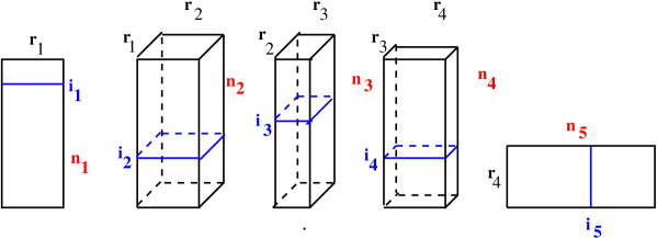
We present numerical tests for high-dimensional cascade problem from [2, 48], which occurs when adjacent genes produce proteins which influence on the expression of a succeeding gene, see Fig. 3.4. Tensor properties of this model, including tensor ranks of CME matrices, have been analyzed theoretically and numerically in [26].

• $d=20$, $M=40$;

• for $m=1$: $w^{m}(\mathbf{x})=0.7$, $\mathbf{z}^{m}=-\delta_{m}$: generation of the first protein;

• for $m=2,...,20$: $w^{m}(\mathbf{x})=\dfrac{x_{m-1}}{5+x_{m-1}}$, $\mathbf{z}^{m}=-\delta_{m}$: succeeding creation reactions;

• for $m=21,...,40$: $w^{m}(\mathbf{x})=0.07\cdot x_{m-20}$, $\mathbf{z}^{m}=\delta_{m-20}$: destruction reactions.

Here $\delta_{m}$ is the $m$-th identity vector, $N_{i}=63$, hence the full grid problem size is about $64^{20}$. The linear QTT format was used for state and time. The dynamical problem was solved until $T=400$ via the restarted global state-time solver after each $T_{0}=15$ time sub-intervals. This means that the global state-time solver applies to $(x,t)$ discretization successively on each coarse time interval of size $T_{0}=15$, so that number of intervals is $T/T_{0}$. The initial state was chosen by $P(0)=\delta_{1}\otimes\cdots\otimes\delta_{1}$, i.e. all copy numbers are zeros. The solution threshold in the discrete $L_{2}$norm for the QTT-rank truncation was chosen as $\varepsilon=10^{-5}$.

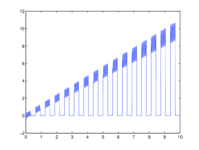
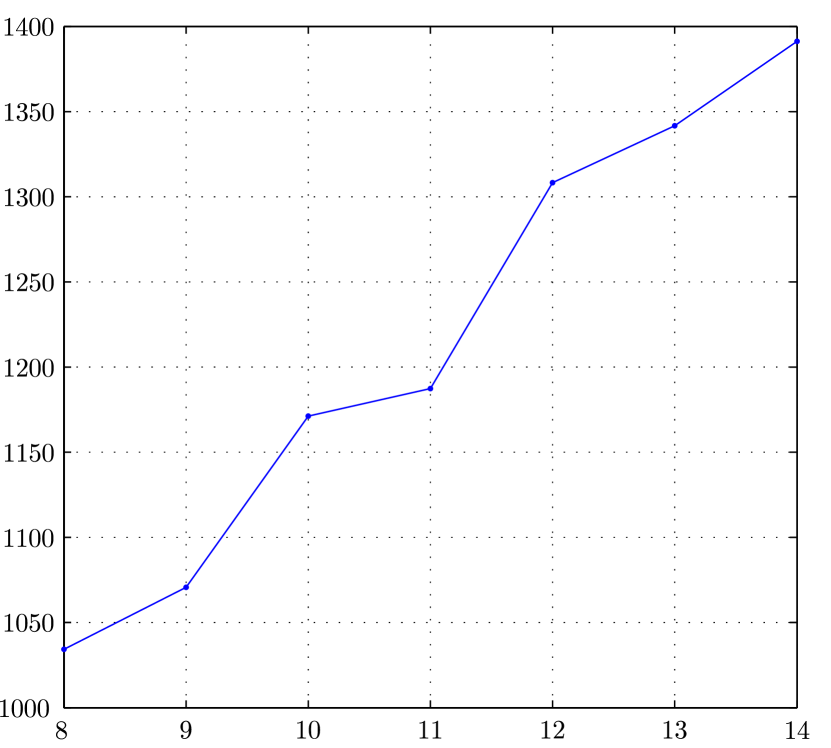
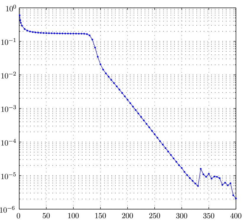
Fig. 3.6 illustrates the $\log N_{t}$ scaling of the solution time for the varying number of time steps, $N_{t}=2^{8},2^{9},...,2^{14}$. Fig. 3.6 shows the convergence of the transient solution to stationary one. This confirms that the chosen time interval $T$ is large enough (long-time dynamics) to catch the steady state with the required precision.

Figure 3.5: CPU time (sec.) vs. $\log N_{t}$.

Figure 3.6: Closeness to the kernel $\dfrac{||AP||}{||P||}(t)$

We conclude that presented results demonstrate the high performance of QTT- and QTT-Tucker formats in tensor computations for multi-dimensional CMEs. For many interesting cases the theoretical rank bounds for the CME matrices have been proven [26]. Numerical tests confirm the logarithmic complexity scaling of the global space-time tensor schemes in both time and space discretization parameters, indicating the potential advantages of this approach for high-dimensional dynamical simulations.

4 Conclusions

The main ingredients and favorable features of the modern tensor numerical methods in applications to multidimensional PDEs have been discussed. We focused on the recent finding of quantized tensor approximation that allows to represent discrete multivariate functions and operators on large $d$-dimensional grids of size $N^{d}$, with log-volume complexity, $O(d\log N)$. We show how this approach can be applied to the low-parametric representation of functions and operators on the examples of nonlinear Hartree-Fock and real-time dynamical master equations.

Other examples on successful applications of tensor numerical methods to parametric/stochastic PDEs, time-dependent parabolic equations, multidimensional eigenvalue problems, the fast lattice summation schemes, superfast data transforms and to integration of singular and highly oscillating functions can be found in references provided.

Acknowledgements. The author gratefully acknowledge Dr. V. Khoromskaia (MPI MiS Leipzig) for useful comments on Section 2 and §3.1 which have led to the substantial improvement of the revised manuscript.

References

- [1] P.-A. Absil, R. Mahony, and R. Sepulchre, Optimization Algorithms on Matrix Manifolds. Princeton University Press, Princeton, NJ, 2008.
- [2] Ammar A., Cueto E., Chinesta F. Reduction of the chemical master equation for gene regulatory networks using proper generalized decompositions. Int. J. Numer. Meth. Biomed. Engng. 2011. V. 00. P. 1–15.
- [3] R. Andreev, and C. Tobler. Multilevel preconditioning and low rank tensor iteration for space-time simultaneous discretization of parabolic PDEs. Tech. Rep. 16, SAM, ETH Zürich 2012.
- [4] M. Bachmayr and W. Dahmen, Adaptive near-optimal rank tensor approximation for high-dimensional operator equations. IGPM Preprint 363, RWTH Aachen, April 2013.
- [5] J. Ballani, L. Grasedyck, and M. Kluge. Black box approximation of tensors in hierarchical Tucker format. Linear Alg. Appl., v. 428, 2013, 639-657. doi:10.1016/j.laa.2011.08.010
- [6] M. Barrault, E. Cancés, W. Hager and Le Bris. Multilevel domain decomposition for electronic structure calculations. J. Comput. Phys. 222, 2007, 86-109.
- [7] H. Bateman and A. Erdelyi, Higher Transcendental Functions, v. 2, MC Graw-Hill Book Comp., New York, Toronto, London, 1988.
- [8] M. Bebendorf. Adaptive cross approximation of multivariate functions. Constructive approximation, v. 34(2), 149-179, 2011.
- [9] Binev P., Cohen A., Dahmen W. et al. Convergence rates for greedy algorithms in reduced basis methods. SIAM J. Math. Anal. 2011. V. 43, 3. P. 1457-1472.
- [10] H. Bateman and A. Erdelyi. Higher Transcendental Functions, v. 2, MC Graw-Hill Book Comp., New York, Toronto, London, 1988.
- [11] Bellman R. E. Dynamic programming. – Princeton University Press, 1957.
- [12] Benner, P. and Breiten, T. Low rank methods for a class of generalized Lyapunov equations and related issues. Numerische Mathematik, 124/3, 441-470, 2013. doi=10.1007/s00211-013-0521-0.
- [13] Benner, P. and Onwunta, A. and Stoll, M. Low Rank Solution of Unsteady Diffusion Equations with Stochastic Coefficients, MPI Magdeburg Preprint, 13-13, 2013. http://www2.mpi-magdeburg.mpg.de/preprints/2013/MPIMD13-13.pdf.
- [14] C. Bertoglio, and B.N. Khoromskij. Low-rank quadrature-based tensor approximation of the Galerkin projected Newton/Yukawa kernels. Comp. Phys. Communications, v. 183(4), 904-912 (2012).
- [15] G. Beylkin and M.J. Mohlenkamp. Numerical operator calculus in higher dimensions. Proc. Natl. Acad. Sci. USA 99 (2002) 10246–10251.
- [16] F.A. Bischoff and E.F. Valeev. Low-order tensor approximations for electronic wave functions: Hartree-Fock method with guaranteed precision. J. of Chem. Phys., 134, 104104-1-10 (2011).
- [17] T. Blesgen, V. Gavini, V. Khoromskaia. Approximation of the electron density of Aluminium clusters in tensor-product format. J. Comp. Phys., 231, No.6, 2012, 2551-2564.
- [18] D. Braess. Asymptotics for the Approximation of Wave Functions by Exponential-Sums. J. Approx. Theory, 83: 93-103, (1995).
- [19] Cancés E., Ehrlacher V., Leliévre T., Convergence of a greedy algorithm for high-dimensional convex nonlinear problems. Mathematical Models and Methods in Applied Sciences. 2011.
- [20] E. Cancés, V. Ehrlacher, and Y. Maday. Periodic Schrödinger operator with local defects and spectral pollution. SIAM J. Numer. Anal. v. 50, No. 6 (2012), pp. 3016-3035.
- [21] W. Dahmen, R. Devore, L. Grasedyck, E. Süli. Tensor-sparsity of solutions to high-dimensional elliptic partial differential equations. IGPM Preprint, RWTH Aachen, July 2014.
- [22] L. De Lathauwer, B. De Moor, J. Vandewalle, On the best rank- and rank- approximation of higher-order tensors. SIAM J. Matrix Anal. Appl., 21 (2000) 1324-1342.
- [23] S.V. Dolgov, and B.N. Khoromskij. Two-level Tucker-TT-QTT format for optimized tensor calculus. SIAM J. on Matr. Anal. Appl., 34(2), 2013, pp. 593-623.
- [24] S.V. Dolgov, B.N. Khoromskij, and D. Savostyanov. Superfast Fourier transform using QTT approximation. J. Fourier Anal. Appl., 2012, vol.18, 5, 915-953.
- [25] S.V. Dolgov, B.N. Khoromskij, and I. Oseledets. Fast solution of multi-dimensional parabolic problems in the TT/QTT formats with initial application to the Fokker-Planck equation. SIAM J. Sci. Comput., 34(6), 2012, A3016-A3038.
- [26] S. Dolgov, and B.N. Khoromskij. Simultaneous state-time approximation of the chemical master equation using tensor product formats. arXiv:1311.3143, 2013; To appear in NLAA 2014, http://dx.doi.org/10.1002/nla.1942.
- [27] S. Dolgov, B.N. Khoromskij, A. Litvinenko, and H.G. Matthies. Computation of the Response Surface in the Tensor Train data format. E-preprint arXiv:1406.2816, 2014.
- [28] Dolgov, S. V. and Oseledets, I. V. Solution of linear systems and matrix inversion in the TT-format. SIAM J. Sci. Comput., 34(5), 2012, A2718-A2739.
- [29] Dolgov S. V., Savostyanov D. V. Alternating minimal energy methods for linear systems in higher dimensions. Part I: SPD systems: arXiv preprint 1301.6068: 2013. http://arxiv.org/abs/1301.6068.
- [30] S. Dolgov, and D.V. Savostyanov. Alternating minimal energy methods for linear systems in higher dimensions. Part II: Faster algorithm and application to nonsymmetric systems. arXiv preprint 1304.1222: 2013.
- [31] Antonio Falcó and Anthony Nouy. Proper generalized decomposition for nonlinear convex prob- lems in tensor Banach spaces. Numerische Mathematik, 121:503-530, 2012.
- [32] V. Ehrlacher, C. Ortner, and A. V. Shapeev. Analysis of boundary conditions for crystal defect atomistic simulations. ArXiv e-prints, 1306.5334, 2013.
- [33] Figueroa L. E., Süli E. Greedy Approximation of High-Dimensional Ornstein-Uhlenbeck Operators. Foundations of Computational Mathematics. 2012. V. 12. P. 573-623.
- [34] L. Frediani, E. Fossgaard, T. Flå and K. Ruud. Fully adaptive algorithms for multivariate integral equations using the non-standard form and multiwavelets with applications to the Poisson and bound-state Helmholtz kernels in three dimensions. Molecular Physics, v. 111, 9-11, 2013.
- [35] I.P. Gavrilyuk, W. Hackbusch and B.N. Khoromskij. Hierarchical Tensor-Product Approximation to the Inverse and Related Operators in High-Dimensional Elliptic Problems. Computing 74 (2005), 131-157.
- [36] I.V. Gavrilyuk, and B.N. Khoromskij. Quantized-TT-Cayley transform to compute dynamics and spectrum of high-dimensional Hamiltonians. Comp. Meth. in Applied Math., v.11 (2011), No. 3, 273-290.
- [37] L. Grasedyck. Hierarchical Singular Value Decomposition of Tensors. SIAM. J. Matrix Anal. and Appl. 31 (2010), 2029.
- [38] L. Grasedyck, Polynomial Approximation in Hierarchical Tucker Format by Vector Tensorization. Preprint 43, DFG/SPP1324, RWTH Aachen, 2010.
- [39] L. Grasedyck, D. Kressner and C. Tobler. A literature survey of low-rank tensor approximation techniques. arXiv:1302.7121v1, 2013.
- [40] M. Griebel, D. Oeltz, and P. Vassilevski, Space-time approximation with sparse grids. SIAM J. Sci. Comput., 28(2):701-727, 2005.
- [41] N. Hale and L.N. Trefethen. Chebfun and numerical quadrature. Sci. China Math. 55 (2012), no. 9, 1749-1760.
- [42] W. Hackbusch. Tensor spaces and numerical tensor calculus. Springer, Berlin, 2012.
- [43] W. Hackbusch. Numerical tensor calculus. Acta Numerica, 2014, pp 651-742.
- [44] W. Hackbusch, B.N. Khoromskij and E.E. Tyrtyshnikov. Hierarchical Kronecker tensor-product approximations. J. Numer. Math. 13 (2005), 119–156.
- [45] W. Hackbusch and B.N. Khoromskij. Low-rank Kronecker product approximation to multi-dimensional nonlocal operators. Part I. Separable approximation of multi-variate functions. Computing 76 (2006), 177-202.
- [46] W. Hackbusch, B.N. Khoromskij, S. Sauter, and E. Tyrtyshnikov. Use of tensor formats in elliptic eigenvalue problems. Numer. Lin. Alg. Appl., v. 19(1), 2012, 133-151.
- [47] R.J. Harrison, G.I. Fann, T. Yanai, Z. Gan, and G. Beylkin. Multiresolution quantum chemistry: Basic theory and initial applications. J. of Chemical Physics, 121 (23): 11587-11598, 2004.
- [48] Hegland M., Burden C., Santoso L. et al. A solver for the stochastic master equation applied to gene regulatory networks. Journal of Computational and Applied Mathematics. 2007. V. 205, 2. p. 708 - 724.
- [49] T. Huckle, K. Waldherr, and T. Schulte-Herbrüggen. Computations in quantum tensor networks. Linear Algebra Appl. 2013; 438:750-781, doi:10.1016/j.laa.2011.12.019.
- [50] Jahnke T., Huisinga W. A Dynamical Low-Rank Approach to the Chemical Master Equation. Bulletin of Mathematical Biology. 2008. V. 70. P. 2283-2302.
- [51] V. Kazeev, and B.N. Khoromskij. Explicit low-rank QTT representation of Laplace operator and its inverse. SIAM Journal on Matrix Anal. and Appl., 33(3), 2012, 742-758.
- [52] V. Kazeev, B.N. Khoromskij, and E.E. Tyrtyshnikov. Multilevel Toeplitz matrices generated by tensor-structured vectors and convolution with logarithmic complexity. SIAM J. Sci. Comput. 35-3 (2013), pp. A1511-A1536.
- [53] V. Kazeev, M. Khammash, M. Nip, and Ch. Schwab. Direct solution of the chemical master equation using quantized tensor train. Research report 04, SAM, ETH Zürich 2013.
- [54] V. Kazeev, O. Reichmann and Ch. Schwab. -DG-QTT solution of high-dimensional degenerate diffusion equations. Techn. Report 2012-11, SAM, ETH Zurich, 2012.
- [55] V. Khoromskaia. Computation of the Hartree-Fock Exchange in the Tensor-structured Format. Comp. Meth. in Applied Math., Vol. 10 (2010), No 2, 204-218.
- [56] V. Khoromskaia. Numerical Solution of the Hartree-Fock Equation by Multilevel Tensor-structured methods. PhD Dissertation, TU Berlin, 2010. http://opus.kobv.de/tuberlin/volltexte/2011/2948/
- [57] V. Khoromskaia. Black-box Hartree-Fock solver by tensor numerical methods. Comp. Meth. in Applied Math., vol. 14 (2014) No. 1, pp. 89-111. doi: 10.1515/cmam-2013-0023.
- [58] V. Khoromskaia, D. Andrae, and B.N. Khoromskij. Fast and Accurate 3D Tensor Calculation of the Fock Operator in a General Basis. Comp. Phys. Communications, 183 (2012) 2392-2404.
- [59] V. Khoromskaia and B.N. Khoromskij. Møller-Plesset (MP2) Energy Correction Using Tensor Factorizations of the Grid-based Two-electron Integrals. Comp. Phys. Communications, 185/1 (2014), 2-10. http://dx.doi.org/10.1016/j.cpc.2013.08.004.
- [60] V. Khoromskaia, B.N. Khoromskij, and R. Schneider. QTT Representation of the Hartree and Exchange Operators in Electronic Structure Calculations. Comp. Meth. in Applied Math., v.11 (2011), No. 3, 327-341.
- [61] V. Khoromskaia, B.N. Khoromskij, and R. Schneider. Tensor-structured calculation of two-electron integrals in a general basis. SIAM J. Sci. Comput., 35(2), 2013, A987-A1010.
- [62] V. Khoromskaia and B. N. Khoromskij. Grid-based lattice summation of electrostatic potentials by assembled rank-structured tensor approximation. arXiv:1405.2270 (submitted).
- [63] V. Khoromskaia, and B.N. Khoromskij. Tensor Approach to Linearized Hartree-Fock Equation for Lattice-type and Periodic Systems. Preprint 62/2014, MPI MiS, Leipzig 2013 (submitted).
- [64] B.N. Khoromskij, Structured Rank- Decomposition of Function-related Tensors in . Comp. Meth. in Applied Math., 6 (2006), 2, 194-220.
- [65] B.N. Khoromskij. Tensor-Structured Preconditioners and Approximate Inverse of Elliptic Operators in . J. Constructive Approx. 30:599-620 (2009).
- [66] B.N. Khoromskij. -Quantics Approximation of - Tensors in High-Dimensional Numerical Modeling. Preprint 55/2009, Max-Planck Institute for Mathematics in the Sciences (MPI MiS), Leipzig 2009. http://www.mis.mpg.de/publications/preprints/2009/prepr2009-55.html.
- [67] B.N. Khoromskij. -Quantics Approximation of - Tensors in High-Dimensional Numerical Modeling. J. Constr. Approx., v.34(2), 2011, 257-289.
- [68] B.N. Khoromskij. Fast and Accurate Tensor Approximation of a Multivariate Convolution with Linear Scaling in Dimension. J. Comput. Appl. Math., 234 (2010) 3122-3139.
- [69] B.N. Khoromskij. Tensors-structured Numerical Methods in Scientific Computing: Survey on Recent Advances. Chemometrics and Intellingent Laboratory Systems, 110 (2012), 1-19.
-
[70]
B.N. Khoromskij.
Introduction to Tensor Numerical Methods in Scientific Computing.
Lecture Notes, University/ETH Zuerich, Preprint 06-2011, Uni.
Zuerich 2011, pp. 1-238.
http://www.math.uzh.ch/fileadmin/math/preprints/0611.pdf - [71] B.N. Khoromskij and V. Khoromskaia. Low Rank Tucker-Type Tensor Approximation to Classical Potentials. Central European J. of Math. 5(3) 2007, 1-28.
- [72] B.N. Khoromskij and V. Khoromskaia. Multigrid Tensor Approximation of Function Related Arrays. SIAM J. on Sci. Comp., 31(4), 3002-3026 (2009).
- [73] B.N. Khoromskij, V. Khoromskaia, and H.-J. Flad. Numerical Solution of the Hartree-Fock Equation in Multilevel Tensor-structured Format. SIAM J. on Sci. Comp., 33(1), 45-65 (2011).
- [74] B.N. Khoromskij, V. Khoromskaia, S.R. Chinnamsetty, and H.-J. Flad. Tensor decomposition in electronic structure calculations on 3D Cartesian grids, J. of Comp. Phys. 228 (2009) 5749-5762.
- [75] B.N. Khoromskij, and S. Miao. Superfast Wavelet Transform Using QTT Approximation. I: Haar Wavelets. Preprint 103/2013, MPI MiS, Leipzig 2013. Comp. Meth. in Applied Math, 2014, DOI 10.1515/cmam-2014-0016.
- [76] B.N. Khoromskij, and I. Oseledets. Quantics-TT collocation approximation of parameter-dependent and stochastic elliptic PDEs. Comp. Meth. in Applied Math., 10(4):34-365, 2010.
- [77] B.N. Khoromskij, and I. Oseledets. Quantics-TT approximation of elliptic solution operators in higher dimensions. Preprint MPI MiS 79/2009, Leipzig 2009.
- [78] B.N. Khoromskij, and I. Oseledets. Quantics-TT approximation of elliptic solution operators in higher dimensions. Russ. J. Numer. Anal. Math. Modelling, v. 26(3), 2011, 303-322.
- [79] B.N. Khoromskij, and I. Oseledets. DMRGQTT approach to the computation of ground state for the molecular Schrödinger operator. Preprint 68/2010, MPI MiS, Leipzig 2010, submitted.
- [80] B.N. Khoromskij, S. Sauter, and A. Veit. Fast Quadrature Techniques for Retarded Potentials Based on TT/QTT Tensor Approximation. Comp. Meth. in Applied Math., v.11 (2011), No. 3, 342 - 362.
- [81] B.N. Khoromskij, and Ch. Schwab. Tensor-Structured Galerkin Approximation of Parametric and Stochastic Elliptic PDEs. SIAM J. Sci. Comp., 33(1), 2011, 1-25.
- [82] O. Koch, Ch. Lubich. Dynamical low rank approximation. SIAM J. Matrix Anal. Appl. 2007. v. 29, 2. P. 434-454.
- [83] T.G. Kolda and B.W. Bader. Tensor Decompositions and Applications. SIAM Review, 51/3, 2009 455-500.
- [84] D. Kressner, M. Steinlechner, and A. Uschmajew. Low-rank tensor methods with subspace correction for symmetric eigenvalue problems. Preprint MATHICSE-ANCHP, Uni. Lausanne, 2013, submitted.
- [85] Kressner D., Tobler C. Preconditioned low-rank methods for high-dimensional elliptic PDE eigenvalue problems. Computational Methods in Applied Mathematics. 2011. V. 11, 3. P. 363-381.
- [86] Kressner, D. and Tobler, C. Krylov Subspace Methods for Linear Systems with Tensor Product Structure. SIAM J. Matrix Anal. Appl., 31(4), 2010, 1688-1714.
- [87] L. Laaksonen, P. Pyykkö and D. Sundholm. Fully numerical Hartree-Fock methods for molecules, Comput. Phys. Rep. 4 (1986) 313–344.
- [88] J.M. Landsberg. Tensors : geometry and applications. Providence, R.I. : American Mathematical Society, 2012.
- [89] C. Le Bris, Computational chemistry from the perspective of numerical analysis. Acta Numerica (2005), 363 - 444.
- [90] Le Bris C., Leliévre T., Maday Y. Results and Questions on a Nonlinear Approximation Approach for Solving High-dimensional Partial Differential Equations. Constr. Approx. 2009. V. 30. P. 621-651.
- [91] Ch. Lubich. From quantum to classical molecular dynamics: reduced models and numerical analysis. Zurich Lectures in Advanced Mathematics, EMS, 2008.
- [92] Lubich C., Rohwedder T., Schneider R., Vandreycken B. Dynamical approximation of hierarchical Tucker and tensor-train tensors: Tech. rep.: University of Tübingen, 2012.
- [93] H. Matthies and A. Keese, Galerkin methods for linear and nonlinear elliptic stochastic partial differential equations. Computer Methods in Applied Mechanics and Engineering, 194 (2005), 1295-1331.
- [94] H. Matthies, A. Litvinenko, O. Pajonk, B.V. Rosić, and E. Zander, Parametric and uncertainty computations with tensor product representations in Uncertainty quantification in scientific computing. A.M. Dienstfrey and R.F. Boisvert, eds., vol. 377 of IFIP Advances in Information and Communication Technology, Springen, Berlin, Heidelberg, 2012, 139-150.
- [95] V. Mazyja, G. Schmidt. Approximate Approximations, Math. Surveys and Monographs, vol. 141, AMS 2007.
- [96] H.-D. Meyer, F. Gatti, and G.A. Worth. Multidimensional Quantum Dynamics: MCTDH Theory and Applications. Willey-VCH, Wienheim, 2009.
- [97] Munsky B., Khammash M. The finite state projection algorithm for the solution of the chemical master equation. The Journal of chemical physics. 2006. V. 124. P. 044104.
- [98] I.V. Oseledets, Tensor train decomposition. SIAM J. Sci. Comp., v. 33(5):2295-2317, 2011.
- [99] I.V. Oseledets. Approximation of matrices using tensor decomposition. SIAM J. Matrix Anal. Appl., 31(4):2130-2145, 2010.
- [100] I.V. Oseledets. Constructive representation of functions in tensor formats. Preprint 2010-04, INM, Moscow, 2010.
- [101] Oseledets I. V., Khoromskij B. N., Schneider R. Efficient time-stepping scheme for dynamics on TT-manifolds. Preprint 24: MPI MIS, 2012. http://www.mis.mpg.de/preprints/2012/preprint201224.pdf. Computing and Visualization in Sci., 2014, to appear.
- [102] I.V. Oseledets, and E.E. Tyrtyshnikov. Breaking the Curse of Dimensionality, or How to Use SVD in Many Dimensions. SIAM J. Sci. Comp., 31 (2009), 3744-3759.
- [103] I.V. Oseledets, and E.E. Tyrtyshnikov. TT-Cross Approximation for Multidimensional arrays. Liner Algebra Appl. 432(1), 70-88 (2010).
- [104] Oseledets I.V., Tyrtyshnikov E.E. Algebraic wavelet transform via quantics tensor train decomposition. SIAM J. Sci. Comput., 2011, 33(3): 1315-1328.
- [105] T. Petersdorff, and C. Schwab. Numerical solution of parabolic equations in high dimensions. Math Model Numer Anal 38, 93-128 (2004).
- [106] D. Perez-Garcia, F. Verstraete, M.M. Wolf, and J.I. Cirac, Matrix Product State Representations. arXiv:quant-ph/0608197v2 14 May 2007.
- [107] M. V. Rakhuba, I. V. Oseledets. Fast multidimensional convolution in low-rank formats via cross approximation. arXiv:1402.5649, 2013.
- [108] Y. Saad, J. R. Chelikowsky, and S. M. Shontz. Numerical Methods for Electronic Structure Calculations of Materials. SIAM Review, v. 52 (1), 2010, 3-54.
- [109] Savostyanov, D. V. and Oseledets, I. V. Fast adaptive interpolation of multi-dimensional arrays in tensor train format. Proceedings of 7th International Workshop on Multidimensional Systems (nDS), University of Poitiers, France, 2011, IEEE, doi:10.1109/nDS.2011.6076873,
- [110] U. Schollwöck. The density-matrix renormalization group in the age of matrix product states, Ann.Phys. 326 (1) (2011) 96-192.
- [111] C. Schwab and R. Todor. Sparse finite elements for elliptic problems with stochastic loading. Numer. Math., 95(4), 707-713, 2003.
- [112] C. Schwab and R. Stevenson. Space-time adaptive wavelet methods for parabolic evolution problems. Math. Comp. 2009; 78(267): 1293-1318.
- [113] G. Szegö, Orthogonal Polynomials. American Mathematical Society, New York, 1959.
- [114] F. Stenger. Numerical methods based on Sinc and analytic functions. Springer-Verlag, 1993.
- [115] Stoll, M. and Breiten, T. A low-rank in time approach to PDE-constrained optimization. MPI Magdeburg Preprint, 13-08, 2013. http://www2.mpi-magdeburg.mpg.de/preprints/2013/MPIMD13-08.pdf.
- [116] L. Tamellini, O. Le Maitre, and A. Nouy. Model reduction based on proper generalized decomposition for the stochastic steady incompressible Navier-Stokes equations. MOX-Report No. 26/2012. Submitted to SIAM J. Sci. Comp.
- [117] L.R. Tucker. Some mathematical notes on three-mode factor analysis. Psychometrika 31 (1966) 279-311.
- [118] F. Verstraete, D. Porras, and J.I. Cirac. DMRG and periodic boundary conditions: A quantum information perspective. Phys. Rev. Lett., 93(22): 227205, Nov. 2004.
- [119] G. Vidal. Efficient classical simulation of slightly entangled quantum computations. Phys. Rev. Lett. 91(14), 2003, 147902-1 147902-4.
- [120] A. Uschmajew Local Convergence of the Alternating Least Squares Algorithm for Canonical Tensor Approximation. SIAM. J. Matrix Anal. & Appl., 33(2), 2012, 639 - 652.
- [121] H. Wang, and M. Thoss. Multilayer formulation of the multiconfiguration time-dependent Hartree theory. J. Chem. Phys. 119 (2003), 1289-1299.
- [122] H.-J. Werner, P.J. Knowles, et al. MOLPRO, Version 2002.10, A Package of Ab Initio Programs for Electronic Structure Calculations.
- [123] S.R. White. Density-matrix algorithms for quantum renormalization groups. Phys. Rev. B, v. 48(14), 1993, 10345-10356.
- [124] Y. Yang, Y. Kurashige, F.R. Manby and G.K.L. Chan. Tensor factorizations of local second-order Møller-Plesset theory. J. Chem. Phys., 134, (pp. 044123:1-13), 2011.
- [125] H. Yserentant. Regularity and Approximability of Electronic Wave Functions. Lecture Notes in Math., 2000, Springer, Dordrecht, 2010.