Abstract

While QCD can provide corrections to the parton distribution function, it cannot produce the distribution. Where is then the starting point for the proton structure function? The only known source is the quark-model wave function for the proton at rest. The harmonic oscillator is used for the trial wave function. When Lorentz-boosted, this wave function exhibits all the peculiarities of Feynman’s parton picture. The time-separation between the quarks plays the key role in the boosting process. This variable is hidden in the present form of quantum mechanics, and the failure to measure it leads to an increase in entropy. This leads to a picture of boiling quarks which become partons in their plasma state.

presented at the Hadron Structure and QCD: from Low to High Energies
(Gatchina, Russia, June 30 July 4, 2014)

1 Introduction

While QED leads to a very successful calculation of the Lamb shift, it cannot provide the hydrogen wave functions with their Rydberg energy levels. Likewise QCD gives corrections to the proton structure function, but it cannot provide the parton distribution to which the corrections are to be made. The only possible starting point is the quark-model wave function for the proton at rest. We can then Lorentz-boost this wave function to see whether it can provide the starting parton distribution with all the peculiarities of Feynman’s parton picture.

Do we then know how to Lorentz-boost the wave function? This question dates back to 1913, when Bohr started worrying about the electron orbits in the hydrogen atom. While Einstein was concerned with how things look to moving observers, he did not ask the question of how those orbits would look to moving observers. He did not ask this question because this did not happen in the real world. Hydrogen atoms moving with relativistic speed did not exist at that time. They still do not exist.

The emergence of the quark model in 1964 changed the world. Like the hydrogen atom, the proton is now a bound state of more fundamental particles called quarks. Unlike the hydrogen atom, the proton can be accelerated to its speed very close to that of light. This historical aspect is illustrated in Fig. 1.

However, do we have wave functions that can be Lorentz-boosted? The present form quantum field theory with Feynman diagrams has been very successful in combining quantum mechanics with special relativity. However, according to Feynman [1], his diagrams are not effective in dealing with bound-state problems. Instead, Feynman suggested the use of harmonic oscillators. He noted that the hadronic mass spectra are consistent with the degeneracy of the three-dimensional harmonic oscillator.

Next question is whether it is possible to construct the oscillator wave functions that can be Lorentz-boosted. It appears that Paul A. M. Dirac was concerned with this question, especially in his papers of 1929, 1945, and 1949 [2, 3, 4].

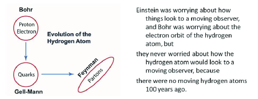
Figure 1: History of bound states in quantum mechanics. The hydrogen atom becomes a proton which can be accelerated to exhibits the peculiarities of Feynman’s parton picture.

In Sec. 2, we integrate those three papers by Dirac to construct that the oscillator wave function that can be Lorentz-boosted. The boosted wave function exhibits all the peculiarities in Feynman’s parton picture [5]. In Sec. 3, it is noted that the time-separation variable plays the key role in the boosting process However, it is a non-measurable hidden variable in the present form of quantum mechanics [6]. It is shown that the confined quarks become plasma-like partons as the hadronic speed approaches that of light.

2 Hadronic wave functions and the parton picture

In 1971, Feynman and his students noted that harmonic oscillator wave functions with their three-dimensional degeneracy can explain the main features of the hadronic spectra [1]. Earlier, in 1969 [5], Feynman proposed his parton picture where a fast-moving hadrons appears like a collection of partons with properties quite different from those of the quarks inside a static hadron.

In their 1971 paper [1], Feynman et al. wrote down a Lorentz-invariant differential equation which can be separated into the Klein-Gordon equation for a free hadron, and a harmonic-oscillator equation for the quarks inside the hadron which determines the hadronic mass. Feynman’s equation of 1971 contains both a running wave for the hadron and a standing wave for the quarks inside the hadron.

Their Lorentz-invariant oscillator equation takes the form

$$\frac{1}{2}\left[\left(\frac{\partial}{\partial x_{\mu}}\right)^{2}-x_{\mu}^{2}\right]\psi\left(x_{\mu}\right)=\lambda\psi\left(x_{\mu}\right),$$ (1)

where $x_{\mu}$ is the four-vector specifying the space-time separation between the quarks. For convenience, we ignore all physical constants such as $c,\hbar$, as well as the spring constant for the oscillator system.

This equation has a solution of the form [3]

$$\psi(z,t)=\frac{1}{\sqrt{\pi}}\exp{\left\{-\frac{1}{2}\left(z^{2}+t^{2}\right)\right\}}.$$ (2)

This solution is Gaussian in both the $z$ and $t$ variables. Is it then possible to attach a physical interpretation to this wave function.

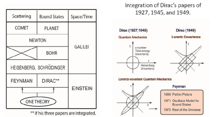
Figure 2: History of scattering and bound states. Feynman diagrams take care of quantum scattering problems in the Lorentz-covariant world. For bound-state problems, it is possible to construct harmonic oscillator wave functions that can be Lorentz-boosted, from Dirac’s ideas given in his papers of 1927, 1945, and 1949.

Indeed, this Gaussian form allows us to integrate three papers Dirac published in his attempt to construct localized wave functions in the Lorentz-covariant world.

• In his 1927 paper [2], Dirac notes there is a time-energy uncertainty relation. However, there are no excitations along the time-like axis, and it is difficult to incorporate this aspect to the Lorentz-covariant world. Dirac calls this uncertainty relations the “c-number” time-energy uncertainty relation.

• In his 1945 paper [3], Dirac considers the Gaussian form of Eq.(2) in his attempt to construct a Lorentz-covariant function. However, he makes no attempts to give a physical interpretation to the time variable in the Gaussian expression.

• In his 1949 paper [4], Dirac considers various forms of relativistic dynamics. Among others, he says there that we can construct relativistic quantum mechanics by constructing a representation of the Poincaré group. He also proposed the light-cone coordinate system.

In a series of papers since 1973 [7], mostly in collaboration with my Marilyn Noz, I was able to integrate the three papers of Dirac listed above [8, 9], and the net result is summarized in Fig. 2. In order to integrate those Dirac papers, we had to fill in the gaps among them.

• For his time variable, Dirac did not mention that the $t$ variable in his Gaussian form of Eq.(2) is the time-separation variable. As the Bohr radius measure the distance between the proton and the electron, there should also be the time-like separation in the relativistic world. This time separation variable is invariant under time translations.

• Then his Gaussian form can be used for his c-number uncertainty relation. There still is the question of whether this c-number nature is consistent with relativity. We can address this question from Wigner’s observation that the internal space-time symmetry of massive particle in isomorphic to the three-dimensional rotation group [10]. Thus, Heisenberg’s position-momentum uncertainty relation can by-pass what happens along the time-like direction.

• Dirac’s papers are like poems, but he never used diagrams. It is possible to combine his 1927 and 1945 papers can be combined into a space-time distribution as specified in Fig. 2. His Lorentz-boost in the light-cone coordinate system is also graphically illustrated in the same figure. It is then straight-forward to the combine his quantum mechanics with relativity.

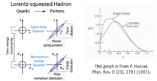
Figure 3: Lorentz-squeezed hadron and quark-parton transition leading to a Gaussian parton distribution. Although there Although there is a general agreement between theory and experiment, the disagreement is substantial. This difference could be corrected by QCD.

If the hadron moves along the $z$ direction with the velocity $v$, the wave function of Eq.(2) becomes

$$\psi_{v}(z,t)=\frac{1}{\sqrt{\pi}}\exp{\left\{-\frac{1}{4}\left[\frac{c-v}{c+v}(z+t)^{2}+\frac{c+v}{c-v}(z-t)^{2}\right]\right\}}.$$ (3)

This corresponds an elliptic distribution given in Fig. 2, where the circular distribution is modulated by Dirac’s light-cone picture of Lorentz boosts. The circle is “squeezed” into the ellipse [7].

According to Fig. 3, the quark distribution becomes concentrated along the immediate neighborhood of one of the light cones as the hadronic speed becomes closer to that of light. In the oscillator regime, the momentum-energy wave function takes the same mathematical form as its space-time counterpart.

Indeed, from these Lorentz-squeezed distributions, it is possible to explain the peculiarities of Feynman’s parton picture [9, 11] First, partons are like free particles, unlike the quarks inside a hadron. Second, the parton distribution function becomes wide-spread as the hadron moves faster. The width of the distribution is proportional to the hadron momentum. Third, the number of partons appears to be infinite. Fourth, the interaction time between the quarks is much longer than the interaction time of one of the quarks with the external signal.

In 1980 [12], Hwa observed that the external signals do not directly interact with the quarks, but with dressed quarks called valons. Thus, if we remove the valon effect, we should be able to measure the distribution of valence quarks. With this point in mind, Hussar in 1981 compared the parton distribution from the boosted oscillator wave function and the experimentally measured distribution [13]. Hussar’s result is given in Fig. 3.

As we can see in this figure, there is a general agreement between the experimental data and the Gaussian curve derived from the Lorentz-boosted wave function from the static quark model. Yet, the disagreement is substantial, especially in the small-x region, and this is the gap QCD has to feel in. This work is yet to be carried out. The wave function needs QCD to make contacts with the real world. Likewise, QCD needs the wave function as a starting point for calculating the parton distribution. They need each other.

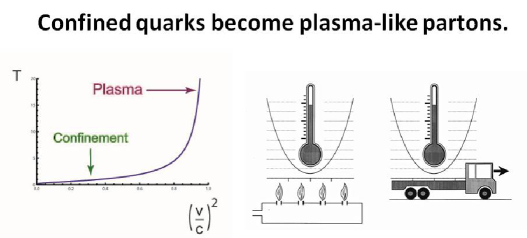
Figure 4: Lorentz boost and boiling quarks. If the hadron is boosted the time-like separation becomes more prominent. If this variable is not measured, the entropy of the system increases [14], leading to a higher temperature. At a sufficiently high temperature the system goes through a phase transition of confined quarks to plasma-like partons.

3 Time-separation variable and the hadronic temperature

Let us go back to Eq.(2). The time-separation variable in the Gaussian form is explained in terms of Dirac’s c-number uncertainty relation in Sec. 2. According to Einstein, this time separation exists wherever there is a space-like separation like Bohr radius. However, this is a hidden variable not measurable in the present form of quantum mechanics. If the variable is not measurable, we have to take a statistical average. In quantum mechanics, we deal with the unmeasurable variable by talking a statistical average, or by integrating the density matrix over the hidden variable. We shall see in this section the consequences in the real world of this hidden time-separation variable.

The squeezed wave function of Eq.(3) can be expanded as [8]

$$\psi_{v}(z,t)=\left[1-\left(\frac{v}{c}\right)^{2}\right]\sum\left(\frac{v}{c}\right)^{n}\phi_{n}(z)\phi_{n}(t),$$ (4)

where $\phi_{n}(z)$ is the oscillator wave function for its k-th excited state. In order to deal with the time-separation variable, we construct the density matrix

$$\rho_{v}(z,t;z^{\prime},t^{\prime})=\psi_{v}(z,t)\psi_{v}^{*}(z^{\prime},t^{\prime}).$$ (5)

Since we are not measuring the $t$ variable, we have to integrate over this hidden variable:

$$\rho_{v}(z;z^{\prime})=\int\rho_{v}(z,t;z^{\prime},t)dt,$$ (6)

leading to

$$\rho_{v}(z;z^{\prime})=\left[1-\left(\frac{v}{c}\right)^{2}\right]\sum\left(\frac{v}{c}\right)^{2n}\phi_{k}(z)\phi_{n}(z^{\prime}).$$ (7)

This operation raises the entropy of the system [14].

The harmonic oscillator can also be thermally excited. The density matrix for the oscillator in its thermally excited state is

$$\rho_{v}(z;z^{\prime})=\left(1-e^{-\hbar\omega/kT}\right)\sum e^{-n\hbar\omega/kT}\phi_{n}(z)\phi_{n}(z^{\prime}).$$ (8)

Let us compare the density matrices given in Eq.(7) and Eq.(8). They become identical if $(v/c)^{2}$ is replaced by $e^{-\hbar\omega/kT}$. The Lorentz boost raises the temperature of the hadron [15], leading to the transition of the confined quarks to plasma-like partons [9]. This phase transition is illustrated in Fig. 4.

References

- [1] R.P. Feynman, M. Kislinger, and F. Ravndal, Phys. Rev. D, 3 (1975) 2706.
- [2] P.A.M. Dirac, Proc. Roy. Soc. (London) A114 (1927) 243.
- [3] P.A.M. Dirac, Proc. Roy. Soc. (London) A183 (1945) 284.
- [4] P.A.M. Dirac, Rev. Mod. Phys. 21 (1945) 392.
-
[5]
R.P. Feynman, Phys. Rev. Lett. 23 (1960), 1415;
R.P. Feynman, in Proceedings of the Third International Conference, Stony Brook, NY, U.S.A. (ed. C. N. Yang, et al.) (Gordon and Breach, New York, 1969) 237. -
[6]
R.P. Feynman Statistical Mechanics(Benjamin/Cummings, Reading,
Massachusetts, 1972);
D. Han, Y.S. Kim, and M.E. Noz, Am. J. Phys. 67 (1999) 61. - [7] Y.S. Kim and M.E. Noz, Phys. Rev. D 8 (1973) 3521.
- [8] Y. S. Kim and M. E. Noz, Theory and Applications of the Poincaré Group (Reidel, Dordrecht, 1986).
- [9] Y.S. Kim and M.E. Noz, Phy. Scie. Int. J. 4 (2014) 1015.
- [10] E. Wigner, Ann. Math. 40 (1939) 149.
- [11] Y.S. Kim and M.E. Noz, Phys. Rev. D 15 (1977) 335.
-
[12]
R. Hwa, Phys. Rev. D 22 (1980) 759;
R. Hwa and M.S. Zahir, Phys. Rev. D 23 (1981) 2539. - [13] P.E. Hussar, Phys. Rev. D 23 (1981) 2781.
- [14] Y.S. Kim and E.P. Wigner Phys. Lett. A 147 (1990) 343.
- [15] D. Han, Y.S. Kim, and M.E. Noz, Phys. Lett. A 144 (1989) 111.