generalmathsymbols
The approximate Loebl–Komlós–Sós Conjecture II:
The rough structure of LKS graphs
Abstract
This is the second of a series of four papers in which we prove the following relaxation of the Loebl–Komlós–Sós Conjecture: For every there exists a number such that for every every -vertex graph with at least vertices of degree at least contains each tree of order as a subgraph.
In the first paper of the series, we gave a decomposition of the graph into several parts of different characteristics; this decomposition might be viewed as an analogue of a regular partition for sparse graphs. In the present paper, we find a combinatorial structure inside this decomposition. In the last two papers, we refine the structure and use it for embedding the tree .
Mathematics Subject Classification: 05C35 (primary), 05C05 (secondary).
Keywords: extremal graph theory; Loebl–Komlós–Sós Conjecture; tree embedding; regularity lemma; sparse graph; graph decomposition.
1 Introduction
This is the second of a series of four papers [HKP+a, HKP+b, HKP+c, HKP+d] in which we provide an approximate solution of the Loebl–Komlós–Sós Conjecture. The conjecture reads as follows.
Conjecture 1.1 (Loebl–Komlós–Sós Conjecture 1995 [EFLS95]).
Suppose that is an -vertex graph with at least vertices of degree more than . Then contains each tree of order .
We discuss the history and state of the art in detail in the first paper [HKP+a] of our series. The main result, which will be proved in [HKP+d], is the approximate solution of the Loebl–Komlós–Sós Conjecture.
Theorem 1.2 (Main result [HKP+d]).
For every there exists a number such that for any we have the following. Each -vertex graph with at least vertices of degree at least contains each tree of order .
In the first paper [HKP+a] we exposed the techniques we use to decompose the host graph. In particular, we saw in [HKP+a, Lemma LABEL:p0.lem:LKSsparseClass] that any graph satisfying the assumptions of Theorem 1.2 may be decomposed into a set of huge degree vertices, regular pairs, an expanding subgraph, and another set with certain expansion properties, which we call the avoiding set. We call this a sparse decomposition of a graph. We will recall the necessary notions from [HKP+a] in Section 3.
Many embedding problems for dense host graphs are attacked using the following three-step approach: (a) the regularity lemma is applied to the host graph, (b) a suitable combinatorial structure is found in the cluster graph, and (c) the target graph is embedded into the combinatorial structure using properties of regular pairs. If we consider the sparse decomposition as a sparse counterpart to (a) then the main result of the present paper, Lemma 5.4, should be regarded as a counterpart to (b). More precisely, for each graph satisfying the assertions of Theorem 1.2 that is given together with its sparse decomposition, Lemma 5.4 gives a combinatorial structure whose building blocks are the elements of the sparse decomposition. As in tree embedding problems in the dense setting (e.g. in [AKS95, PS12]), the core of this combinatorial structure is a well-connected matching consisting of regular pairs. We call such matchings regularized.
With the structure given by Lemma 5.4, one can convince oneself that the tree from Theorem 1.2 can be embedded into the host graph, and indeed we provide such motivation in Section 5.1. However, the rigorous argument is far from trivial. One needs to refine the structure found here, which is done in [HKP+c]. For this reason, we call the output of Lemma 5.4 the rough structure. In the last paper [HKP+d] of our series we will develop embedding techniques for trees, and finally prove Theorem 1.2.
2 Notation and preliminaries
2.1 General notation
The set of the first positive integers is denoted by *@. We frequently employ indexing by many indices. We write superscript indices in parentheses (such as ), as opposed to notation of powers (such as ). We use sometimes subscripts to refer to parameters appearing in a fact/lemma/theorem. For example refers to the parameter from Theorem 1.2. We omit rounding symbols when this does not affect the correctness of the arguments.
Table 2.1 shows the system of notation we use in the series.
| lower case Greek letters | small positive constants () |
|---|---|
| reserved for embedding; | |
| upper case Greek letters | large positive constants () |
| one-letter bold | sets of clusters |
| bold (e.g., ) | classes of graphs |
| blackboard bold (e.g., ) | distinguished vertex sets except for |
| which denotes the set | |
| script (e.g., ) | families (of vertex sets, “dense spots”, and regular pairs) |
| (=nabla) | sparse decomposition (see Definition 3.5) |
We write *VG@ and *EG@ for the vertex set and edge set of a graph , respectively. Further, *VG@ is the order of , and *EG@ is its number of edges. If are two, not necessarily disjoint, sets of vertices we write *EX@ for the number of edges induced by , and *EXY@ for the number of ordered pairs such that . In particular, note that .
*DEG@*DEGmin@*DEGmax@ For a graph , a vertex and a set , we write and for the degree of , and for the number of neighbours of in , respectively. We write for the minimum degree of , , and for two sets . Similar notation is used for the maximum degree, denoted by . The neighbourhood of a vertex is denoted by *N@. We set . The symbol is used for two graph operations: if is a vertex set then is the subgraph of induced by the set . If is a subgraph of then the graph is defined on the vertex set and corresponds to deletion of edges of from . Any graph with zero edges is called empty graphempty. A family of pairwise disjoint subsets of is an ensemble*ENSEMBLE@-ensemble-ensemble in if for each .
Finally, *trees@ denotes the class of all trees of order .
2.2 Regular pairs
Given a graph and a pair of disjoint sets the density*D@density of the pair is defined as
For a given , a pair of disjoint sets is called an regular pair-regular pair if for every , with , . If the pair is not -regular, then we call it irregular-irregular.
We shall need a useful and well-known property of regular pairs.
Fact 2.1.
Suppose that is an -regular pair of density . Let be sets of vertices with , , where . Then the pair is a -regular pair of density at least .
The regularity lemma [Sze78] has proved to be a powerful tool for attacking graph embedding problems; see [KO09] for a survey.
Lemma 2.2 (Regularity lemma).
For all and there exist such that for every the following holds. Let be an -vertex graph whose vertex set is pre-partitioned into sets , . Then there exists a partition of , , with the following properties.
-
(1)
For every we have , and .
-
(2)
For every and every either or .
-
(3)
All but at most pairs , , , are -regular.
We shall use Lemma 2.2 for auxiliary purposes only as it is helpful only in the setting of dense graphs (i.e., graphs which have vertices and edges).
2.3 LKS graphs
*LKSgraphs@
It will be convenient to restrict our attention to a class of graphs which is in a way minimal for Theorem 1.2. Write *LKSgraphs@ for the class of all -vertex graphs with at least vertices of degrees at least . With this notation Conjecture 1.1 states that every graph in contains every tree from .
Given a graph , denote by *S@ the set of those vertices of that have degree less than and by *L@ the set of those vertices of that have degree at least . When proving Theorem 1.2, we may of course restrict our attention to LKS-minimal graphs, that is, to graphs that are edge-minimal with respect to belonging to . It is easy to show that in each such graph the set is independent, all the neighbours of every vertex with have degree exactly , and . It turns out that our main decomposition result [HKP+a, Lemma LABEL:p0.lem:LKSsparseClass] outputs a graph with slightly weaker properties than being LKS-minimal. Let us therefore introduce the following class of graphs.
Definition 2.3.
Suppose that , and . Let *LKSsmallgraphs@ be the class of those graphs for which we have the following three properties:
-
(i)
All the neighbours of every vertex with have degrees at most .
-
(ii)
All the neighbours of every vertex of have degree exactly .
-
(iii)
We have .
3 Decomposing sparse graphs
In [HKP+a] we introduced the notion of sparse decomposition, and proved that every graph can be (almost perfectly) decomposed. We define the sparse decomposition after introducing its basic building blocks: dense spots and avoiding sets. For motivation and more details we refer the reader to [HKP+a, Section LABEL:p0.ssec:class-black], of which this section is a condensed version.
We start by defining dense spots. These are bipartite graphs having positive density, and will (among other things) serve as a basis for regularization.
Definition 3.1 (dense spot-dense spot, nowhere-dense-nowhere-dense).
Suppose that and . An -dense spot in a graph is a non-empty bipartite subgraph of with and . We call a graph -nowhere-dense if it does not contain any -dense spot.
When the parameters and are irrelevant, we refer to simply as a dense spot.
Note that dense spots do not have any specified orientation. That is, we view and as the same object.
Definition 3.2 (-dense cover).
dense cover Suppose that and . An -dense cover of a given graph is a family of edge-disjoint -dense spots such that .
We now define the avoiding set. Informally, a set of vertices is avoiding if for each set of size up to (where is a large constant) and each vertex there is a dense spot containing and almost disjoint from . Favourable properties of avoiding sets for embedding trees are shown in [HKP+a, Section LABEL:p0.sssec:whyavoiding].
Definition 3.3 (avoiding-avoiding set).
Suppose that , and . Suppose that is a graph and is a family of dense spots in . A set is -avoiding with respect to if for every with the following holds for all but at most vertices . There is a dense spot with that contains .
We can now introduce an auxiliary notion of bounded decomposition on which we can build the key concept of sparse decomposition (see below). The main result in [HKP+a] tells us that every graph has an almost perfect sparse decomposition. This sparse decomposition (and the bounded decomposition included in it) will provide us with control on the behaviour of the different edge and vertex sets involved, and thus be helpful to embed the tree.
Definition 3.4 (bounded decomposition-bounded decomposition).
Suppose that and and . Let be a partition of the vertex set of a graph . We say that is a -bounded decomposition of with respect to if the following properties are satisfied:
-
1.
is a -nowhere-dense subgraph of with .
-
2.
is a family of disjoint subsets of .
-
3.
is a subgraph of on the vertex set . For each edge there are distinct and from , and . Furthermore, forms an -regular pair of density at least .
-
4.
We have for all .
-
5.
is a family of edge-disjoint -dense spots in . For each all the edges of are covered by (but not necessarily by ).
-
6.
If contains at least one edge between then there exists a dense spot such that and .
-
7.
For all there is a set so that either or . For all and we have .
-
8.
is a -avoiding subset of with respect to the family of dense spots .
We say that the bounded decomposition respects the avoiding threshold avoiding threshold if for each we either have , or .
The members of are called clusterclusters. Define the cluster graph *Gblack@ as the graph on the vertex set that has an edge for each pair which has density at least in the graph . Further, we define the graph *GD@ as the union (both edge-wise, and vertex-wise) of all dense spots .
We now enhance the structure of bounded decomposition by adding one new feature: vertices of very large degree.
Definition 3.5 (sparse decomposition-sparse decomposition).
Suppose that and and . Let be a partition of the vertex set of a graph . We say that is a -sparse decomposition of with respect to if the following hold.
-
1.
, , , where is spanned by the edges of , , and edges incident with ,
-
2.
is a -bounded decomposition of with respect to .
If the parameters do not matter, we call simply a sparse decomposition, and similarly we speak about a bounded decomposition.
Definition 3.6 (captured edgescaptured edges).
In the situation of Definition 3.5, we refer to the edges in as captured edgescaptured by the sparse decomposition. We write *Gclass@ for the subgraph of on the vertex set which consists of the captured edges. Likewise, the captured edges of a bounded decomposition of a graph are those in .
It will be useful to have the following shorthand notation at hand.
Definition 3.7 ( and ).
Suppose that and and . We define *G@ to be the class of all quadruple with the following properties:
-
(i)
is a graph of order with ,
-
(ii)
is a bipartite subgraph of with colour classes and and with ,
-
(iii)
is a -dense cover of ,
-
(iv)
is a -ensemble in , and ,
-
(v)
for each and for each .
Those , and satisfying all conditions but (ii) and the last part of (iv) will make up the triples of the class *G@.
4 Augmenting a matching
In previous papers [AKS95, Zha11, PS12, Coo09, HP15] concerning the LKS Conjecture in the dense setting the crucial turn was to find a matching in the cluster graph of the host graph possessing certain properties. We will prove a similar “structural result” in Section 5. In the present section, we prove the main tool for Section 5, namely Lemma 4.8. All statements preceding Lemma 4.8 are only preparatory. The only exception is (the easy) Lemma 4.4 which is recycled later, in [HKP+c].
4.1 Regularized matchings
We prove our first auxiliary lemma on our way towards Lemma 4.8.
Lemma 4.1.
For every and there is a number such that for every there exists a number such that for each the following holds.
For every there are , and such that
-
(1)
,
-
(2)
and , where and are the colour classes of , and
-
(3)
is an -regular pair in of density .
Proof.
Let , , and be given. Applying Lemma 2.2 to and , we obtain numbers and . We set
| (4.1) |
and given , we set
Now suppose we are given and .
Property (i) of Definition 3.7 gives that , and Property (ii) says that . So . Averaging over all dense spots in the dense cover of we find a dense spot such that
| (4.2) |
Without loss of generality, we assume that
| (4.3) |
as otherwise one can just interchange the roles of and . Then,
| (4.4) |
As covers , has an edge with for some and . Set and . Then directly from the definition of and since is a -dense spot, we obtain that
| (4.5) |
Also, since , we have
| (4.6) |
This enables us to bound the size of as follows.
| (4.7) | ||||
Similarly,
| (4.8) |
Applying Lemma 2.2 to with prepartition we obtain a collection of sets , with . By (4.7), and (4.8), we have that for every . It is easy to deduce from (4.5) that there is at least one -regular (and thus -regular) pair , , , with . Indeed, it suffices to count the number of edges incident with , lying in -irregular pairs or belonging to too sparse pairs. The number of these “bad” edges is strictly smaller than
Thus not all edges between and are bad in the sense above. This finishes the proof of Lemma 4.1. ∎
Instead of just one pair , as it is given by Lemma 4.1, we shall later need several disjoint pairs for embedding larger trees. For this purpose we introduce the following definition, generalizing the notion of a matching in the cluster graph in the traditional regularity setting.
Definition 4.2 (-regularized matching).
Suppose that and . A collection of ordered pairs with is called an regularized@regularized matching-regularized matching of a graph if
-
(i)
for each ,
-
(ii)
induces in an -regular pair of density at least , for each , and
-
(iii)
all involved sets and are pairwise disjoint.
Sometimes, when the parameters do not matter (as for instance in Definition 4.5 below) we simply call it a regularized matching.
For a regularized matching , we shall write *V1@, , , and . Furthermore, we set *V1@, , , and . As these definitions suggest, the orientations of the pairs are important. The sets and are called *VERTEX@-vertexvertex@-vertex-vertices and the pair is an *EDGE@-edgeedge@-edge-edge.
We say that a regularized matching absorbabsorbs a regularized matching if for every there exists such that and . In the same way, we say that a family of dense spots absorbabsorbs a regularized matching if for every there exists such that and .
We later need the following easy bound on the size of the elements of .
Fact 4.3.
Suppose that is an -regularized matching in a graph . Then for each .
Proof.
Let for example . The maximum degree of is at least as large as the average degree of the vertices in , which is at least . ∎
The second step towards Lemma 4.8 is Lemma 4.4. Whereas Lemma 4.1 gives one dense regular pair, in the same setting Lemma 4.4 provides us with a dense regularized matching.
Lemma 4.4.
For every and there exists such that for every there is a number such that the following holds for every .
For each there exists an -regularized matching of such that
-
for each there are , and such that and , and
-
.
Proof.
Now let . Let be an inclusion-maximal -regularized matching with property . We claim that
| (4.9) |
Indeed, suppose the contrary. Then the bipartite subgraph of induced by the sets and satisfies Property (ii) of Definition 3.7, with . So, we have that .
4.2 Augmenting paths for matchings
We now prove the main lemma of Section 4, namely Lemma 4.8. We will use an augmenting path technique for our regularized matchings, similar to the augmenting paths commonly used for traditional matching theorems. For this, we need the following definitions.
Definition 4.5 (Alternating path, augmenting pathalternating pathaugmenting path).
Suppose that and . Given an -vertex graph , and a regularized matching , we call a sequence (where is arbitrary) a -alternating path for from if for all we have
-
(i)
and the sets are pairwise disjoint,
-
(ii)
and ,
-
(iii)
, and
-
(iv)
, for each . \suspendenumerate If in addition there is a set of disjoint subsets of such that \resumeenumerate[[(i)]]
-
(v)
,
then we say that is a -augmenting path for from to .
The number is called the length of alternating path length of (or of ).
Next, we show that a regularized matching either has an augmenting path or admits a partition into two parts so that only few edges cross these parts in a certain way.
Lemma 4.6.
Given an -vertex graph with , a number , a regularized matching , a set , and a set of disjoint subsets of , one of the following holds:
-
(M1)
There is a regularized matching with
-
(M2)
has a -augmenting path of length at most from to .
Proof.
If then (M1) is satisfied for . Let us therefore assume the contrary.
Choose a -alternating path for with maximal.
Now, let be maximal with . Then . Moreover, as for all , we have that and thus
| (4.10) |
Let consist of all -edges with . Then, by the choice of ,
| (4.11) |
Furthermore, if (that is, if ) then
| (4.12) |
Thus, if , we see that is satisfied for . So, assume the contrary. Then, by (4.10), there is an index for which
and thus, is a -augmenting path for . This proves (M2). ∎
The aim of this section is to find a regularized matching covering as many vertices from the graph as possible. This is done by iteratively improving a matching. Below, Lemma 4.7 provides with such an iterative step: given a regularized matching we either find (II) a better regularized matching , or there is (I) a natural barrier to finding such a matching. This barrier is a separation of the previous regularized matching into two blocks ( and ) such that very few edges “cross” this separation. The absence of such a separation guarantees the existence of an augmenting path for , which can be used to find a better regularized matching. This matching has (C1) to improve substantially and (C2) respect the structure of the graph and of .
Lemma 4.7.
For every and there is a number such that for every there is a number such that for every there is a number such that for every there is such that the following holds for every and every .
Let be a graph of order with , with an -regularized matching and with a -dense cover that absorbs . Let , and let be an -ensemble in with . Assume that for each and each .
Then one of the following holds.
-
(I)
There is a regularized matching such that
-
(II)
There is an -regularized matching such that
-
(C1)
, and , and
-
(C2)
for each there are sets , and a dense spot such that and .
-
(C1)
Proof.
We divide the proof into five steps.
Step 1: Setting up the parameters.
Suppose that and are given. For , we define the auxiliary parameters
| (4.13) |
and set
Given , we define
Then, given , for , we define the further auxiliary parameters
which are given by Lemma 4.4 for input parameters , , , and . Set
Given the next111in the order of quantification from the statement of the lemma input parameter , Lemma 4.4 for parameters as above and the final input yields , set
Step 2: Finding an augmenting path.
We apply Lemma 4.6 to , , , and . Since corresponds to (I), let us assume that the outcome of the lemma is . Then there is a -augmenting path for starting from such that .
Our aim is now to show that (II) holds.
Step 3: Creating parallel matchings.
Inductively, for we shall define auxiliary bipartite induced subgraphs with colour classes and that satisfy
-
(a)
and -regularized matchings that satisfy
-
(b)
,
-
(c)
for each there are a dense spot and a set (or a set if ) such that and ,
-
(d)
, and
-
(e)
for each edge , if .
We take as the induced bipartite subgraph of with colour classes and . Definition 4.5 (v) together with (4.13) ensures (a) for . Now, for , suppose is already defined. Further, if suppose also that is already defined. We shall define , and, if , we shall also define .
Observe that , because of (a) and the assumptions of the lemma. So, applying Lemma 4.4 to and noting that , we obtain an -regularized matching that satisfies conditions (b)–(d).
Step 4: Harmonising the matchings.
Our regularized matchings will be a good base for constructing the regularized matching we are after. However, we do not know anything about for the -edges . But this term will be crucial in determining how much of gets lost when we replace some of its -edges with -edges. For this reason, we refine in a way that its -edges become almost equal-sized.
Formally, we shall inductively construct regularized matchings such that for we have
-
(A)
is an -regularized matching,
-
(B)
absorbs ,
-
(C)
if and with then , and
-
(D)
if and .
Set . Clearly (B) holds for , (A) is easy to check, and (C) is void. Finally, Property (D) holds because of (d). Suppose now and that we already constructed matchings satisfying Properties (A)–(D).
So, we can choose a subset such that for each . Now, for each write , and choose a subset of of size . Set
| (4.17) |
In order to verify (D), it suffices to observe that
Step 5: The final matching.
Suppose that with for some . Then, set . Also, choose a set of cardinality . This is possible by (C). By (4.17) we deduce that
| (4.18) |
We consider the set consisting of all -edges with .
Set
By the assumption of the lemma, for every there are an edge and a dense spot such that
| and . | (4.19) |
Since is -regularized, Fact 2.1 implies that is an -regularized matching. Set
It is easy to check that is an -regularized matching. Using (4.19) together with (B) and (c), we see that (C2) holds for .
In order to see (C1), we calculate
In (sum2), consider an arbitrary term corresponding to . By the definition of , the term is zero. To treat the term , we recall that and (in the definition of ). This gives that . This leads to
Using the fact that the last calculation also implies that
since by assumption. ∎
Iterating Lemma 4.7 we prove the main result of the section.
Lemma 4.8.
For every and there exists a number such that for every , there are such that for each there exists a number such that the following holds for every and .
Let be a graph of order , with . Let be a -dense cover of , and let be an -regularized matching that is absorbed by . Let be a -ensemble in with . Let . Assume that for each , and for each we have that
| (4.20) |
Then there exists an -regularized matching such that
-
(i)
,
-
(ii)
for each there are sets , and a dense spot such that and , and
-
(iii)
can be partitioned into and so that
Proof.
Let and be given. Let be the output given by Lemma 4.7 for input parameters and .
Set , set , and for , inductively define to be the output given by Lemma 4.7 for the further input parameter (keeping and fixed). Then for all . Set .
Given we set for , and set . Clearly,
| (4.21) |
Now, for , let be given by Lemma 4.7 for input parameters , , and . For , set . Let .
Given , let be the maximum of the lower bounds given by Lemma 4.7 for input parameters , , , , , for .
Suppose now we are given , , , and . Suppose further that . Let be maximal subject to the condition that there is a matching with the following properties:
-
(a)
is an -regularized matching,
-
(b)
,
-
(c)
, and
-
(d)
for each there are sets , and a dense spot such that and .
Observe that such a number exists, as for we may take . Also note that because of (b).
We now apply Lemma 4.7 with input parameters , , , , to the graph with the -dense cover , the -regularized matching , the set
and the -ensemble
Lemma 4.7 yields a regularized matching which either corresponds to as in Assertion (I) or to as in Assertion (II). Note that in the latter case, the matching actually constitutes an -regularized matching fulfilling all the above properties for . In fact, (b) and (c) hold for because of , and it is not difficult to deduce (d) from and from (d) for . But this contradicts the choice of . We conclude that we obtained a regularized matching as in Assertion (I) of Lemma 4.7.
Thus, in other words, can be partitioned into and so that
| (4.22) |
Set . Then is -regularized by (a). Note that Assertion (i) of the lemma holds by (4.21) and by (c). Assertion (ii) holds because of (d).
Since
and because of (4.22) we know that in order to prove Assertion (iii) it suffices to show that
sends at most edges to the rest of the graph. For this, it would be enough to see that , since by assumption, has maximum degree .
To this end, note that by assumption, . Further, the definition of implies that for each we have that . Combining these two observations, we obtain that
as desired.
∎
5 Rough structure of LKS graphs
In this section we give a structural result for graphs , stated in Lemma 5.4. Similar structural results were essential also for proving Conjecture 1.1 in the dense setting in [AKS95, PS12]. There, a certain matching structure was proved to exist in the cluster graph of the host graph. This matching structure then allowed us to embed a given tree into the host graph. We motivate the structure asserted by Lemma 5.4 in more detail in Section 5.1.
Naturally, in our possibly sparse setting the sparse decomposition of will enter the picture (instead of just the cluster graph of . For more on sparse decomposition, see [HKP+a]). There is an important subtlety though: we may need to “re-regularize” the cluster graph of . In this case, we have to find another regularization of parts of , partially based on . Lemma 4.8 is the main tool to this end. The re-regularization is captured by the regularized matchings and .
Let us note that this step is one of the biggest differences between our approach and the announced solution of the Erdős–Sós Conjecture by Ajtai, Komlós, Simonovits and Szemerédi. In other words, the nature of the graphs arising in the Erdős–Sós Conjecture allows a less careful approach with respect to regularization, still yielding a structure suitable for embedding trees. We discuss the necessity of this step in further detail in Section 5.2. The main result of this paper Lemma 5.4, is given in Section 5.3.
5.1 Motivation for and intuition behind Lemma 5.4
Recall that [HKP+a, Lemma LABEL:p0.lem:LKSsparseClass] asserts that each graph satisfying the conditions of Theorem 1.2 has a sparse decomposition which captures almost all its edges. With this pre-processing at hand, we want Lemma 5.4 to provide specific structural properties of under which we could make the embedding of the tree work. The complexity of these assertions (which span more than half a page) stems from the complicated nature of the sparse decomposition, and from the delicate features of the embedding techniques (worked out in [HKP+d, Section LABEL:p3.sec:embed]). In this section we try to explain and motivate the key assertions of Lemma 5.4. The reader may skip the section at his or her convenience. The only bit from this section needed for the main result is Definition 5.3.
At this stage, let us introduce informally the notion of fine partition which we use to cut up the tree . Let . We find a constant number of cut vertices of so that the components (which we refer to as shrubs) in the remainder of are of order at most . The cut vertices will decompose into two sets and so that the distance from any vertex of to any vertex in is odd. It can be shown that we can do the cutting so that each shrub either neighbours only one cut vertex from , or it neighbours two, in which case both these cut vertices are in . Thus, the set of all shrubs can be decomposed as depending on the cut vertices that surround individual shrubs. The last property of the fine partition we shall use is that
| (5.1) |
The quadruple is then called a -fine partition of . The full definition which includes several additional properties is given in [HKP+d, Section LABEL:p3.ssec:cut].
As said earlier, Lemma 5.4 is an extensive generalization of previous structural results on the LKS Conjecture in the dense setting. So, as a starting point for our motivation, let us explain the structural result Piguet and Stein [PS12] use to prove the dense approximate version of the LKS Conjecture.
Theorem 5.1 ([PS12]).
For every and there exists a number such that for every and we have the following. For every graph contains each tree from .
Here, of course, the structure we work with is encoded in the cluster graph (in the sense of the original regularity lemma) of the graph . Note that , where is the number of clusters and . The main structural result of Piguet and Stein then reads as follows.
Informal Lemma 5.2 ([PS12, Lemma 8], simplified).
Suppose that and let us write . Then we have at least one of the following two cases.
-
There exists a matching and an edge so that , for .
-
There exists a matching and an edge with , and . Further,
(5.2)
Piguet and Stein use structures (H1) and (H2) to embed any given tree into using the regularity method. A comprehensive description of the embedding procedure is given in Sections 3.6 and 3.7 in [PS12]. The embedding itself is quite technical but it follows a relatively pedestrian strategy which we present next. The regularity method tells us that a regular pair can be filled up by an arbitrary family of shrubs, provided that the colour classes of these shrubs (viewed as one bipartite graph) do not overfill the end-clusters of that regular pair. The degree conditions in Informal Lemma 5.2 suggest that we will utilize the clusters of and of . More precisely, some of the shrubs will be accommodated in the edges of the matching . Suppose next that we would like to proceed with embedding some shrubs using a cluster . This can be done as follows. Using the high-degree property of we can find a cluster adjacent to that is not filled up completely by the image of . We then use the pair to accommodate further shrubs. We keep embedding by mapping to (in ) or to (in ), to or to , and the shrubs pendent from these cut-vertices either into the regular edges of , or to edges incident to clusters as described above. Thus, the degree conditions in Informal Lemma 5.2 guarantee that we can accommodate shrubs of total order up to from , , and . The degree bound for guarantees that we can embed shrubs of total order up to from , recall that this is sufficient, thanks to (5.1). The fact that or forms an edge allows us to make connections between images of and .
We do not need a counterpart of (5.2) for . The reason is that we can schedule our embedding process in such a way that when we use the high-degree property of we have already exhausted the degree from to .
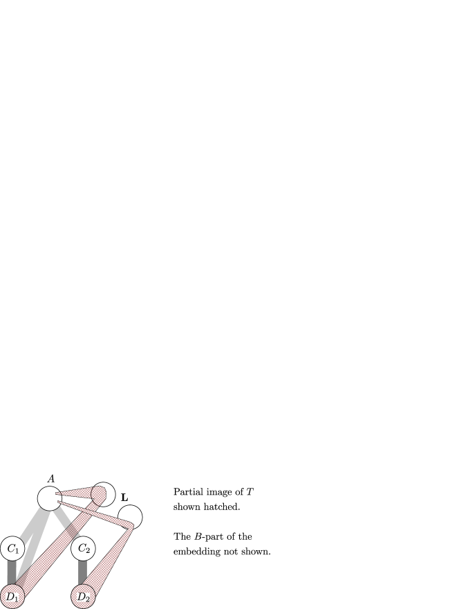
So far, we have not explained the role of condition (5.2). We include a relatively detailed explanation in Figure 5.1. However, this condition is independent of the rest of the argument, and it may be sufficient for the reader to take granted that (5.2) is crucial for the embedding to work.
We now try to give an analogue to Informal Lemma 5.2 in the sparse setting when the structure of is encoded in the sparse decomposition rather than in the cluster graph. Recall that in the dense setting sets suitable for embedding shrubs were clusters of a regular matching (that is, ), and clusters of large degree (that is, ). In the sparse setting, in addition to using a suitable matching of regular pairs and large degree vertices we can make use of two further sets for embedding shrubs: (as explained in [HKP+a, Section LABEL:p0.sssec:whyGexp]) and the set (as explained in [HKP+a, Section LABEL:p0.sssec:whyavoiding]). Thus, the counterpart of clusters , and from Informal Lemma 5.2 is the set of vertices, which have degree at least into the set .333The rather different looking formal definition of is given in (5.4). Below, we give an explanation for this difference. Likewise, the counterpart of cluster in Informal Lemma 5.2 are vertices of , which have degree at least into .444The formal definition of is given again in (5.4). We see that a sparse counterpart to would be two disjoint well-connected sets . In Lemma 5.4 we achieve this in one of two possible ways. One way is finding a large regularized matching inside ; one can then take and . This corresponds to in Lemma 5.4(h). Next, suppose that induces sufficiently many edges. Then we take and to be a bipartition of corresponding to a maximum cut. Hence, the sets and are again well-connected. This corresponds to the case in in Lemma 5.4(h). Similarly, if the sets and are well-connected, we are on a good track to getting a sparse version of .
It remains to translate condition (5.2). The right counterpart to this condition is
| (5.3) |
The actual statement of Lemma 5.4 deviates quite substantially from the informal account given above. So, let us now state an informal version of Lemma 5.4. After that, we explain how it relates to the description above. Also, we mark the correspondence between this informal version and the actual lemma by using the same numbering. In particular, assertions (d), (f), (g) in Lemma 5.4 are needed for reasons that cannot be explained in this high-level overview and are not reflected in the informal version. Further, statement of (c’) of our informal lemma carries only half of the information compared to the full version in Lemma 5.4.
Let us now give the actual definitions of the sets , . Later, we explain how these definitions imply the features described above.
Definition 5.3.
Suppose that , and . Suppose that is a graph with a -sparse decomposition
with respect to and . Suppose further that are regularized matchings in . We then define the triple *XA@ *XB@ *XC@ by setting
| (5.4) | ||||
where on the second line is defined by
| (5.5) |
It is enough to restrict ourselves for the proof to the class . We intentionally leave out (or simplify) almost all numerical parameters in this informal statement.
Informal version of Lemma 5.4.
Suppose is a sparse decomposition of a graph . We write . Then there exist regularized matchings and , such that for the sets and defined as in Definition 5.3 we have
-
(a)
,
-
(b)
,
-
for each we have that or ,
-
(e)
,
-
(h)
if induces almost no edges and does not contain a substantial regularized matching555The exact quantification of “almost no edges” and “substantial regularized matching” does not in guarantee the former property to imply the latter. See also Remark 5.5 then there is a substantial amount of edges between and .
The regularized matching from the lemma plays the role of in the motivation above. It remains to justify the dissimilarities between the statement of the lemma and the text above. The first discrepancy is that the definitions of the sets and in (5.4) are quite different from the ones in the motivation above. The other discrepancy is a seeming absence of (5.3) in the statement. As for the first issue, consider an arbitrary vertex . Property (e) tells us that sends no edges to . As , we have that , as needed. Next, consider a vertex . The fact that together with the definition of immediately gives that , again as needed.
Let us now turn to deriving (5.3). This property is required only for the counterpart of . So, we can assume that we do not have the counterpart of , that is, the set induces (almost) no edges. Let us now consider an arbitrary regular pair in . First assume that . Then (b) tells us that . We then have by Property (e), as needed for (5.3). Next, assume that . Then Definition 2.3(ii) (together with (c’) of our informal lemma) tells us that at least one of and is contained in . Say this is . We then have . But the absence of edges inside tells us that , again as needed for (5.3).
5.1.1 Rough versus fine structure
In the dense case [PS12] we can proceed with embedding using the regularity method immediately after having established a statement like Informal Lemma 5.2. That is, we can zigzag-embed consecutive cut vertices of in , or . When we arrive at a shrub stemming from cut vertex embedded to a cluster (that is, , , , or ) we can use or to find an edge such that and the pair has not been filled-up. Then, (i) using that we traverse from to , (ii) we embed in , and (iii) if is an internal shrub, we again use that to traverse back666As said at the beginning of Section 5.1, if is internal, then both of its neighboring cut vertices are in . In particular, the distance between these two cut vertices is even. That means that to traverse back to , we really use the pair . to and continue embedding cut vertices in or .
In the current setting of the sparse decomposition, the structure given by Lemma 5.4 would allow us to carry out counterparts to (i) and (ii) (even though there is a number of technical obstacles). That is, we would be able to embed consecutive cut vertices, to traverse to locations suitable for shrubs and to embed these shrubs. However, carrying a counterpart to (iii) is a major problem. The symmetry-based argument from the dense case “if is an edge then is an edge and thus we can traverse in both directions” does not work when the shrub is not to be embedded in a cluster, but in a subset of or . This is going to be addressed in [HKP+c], where we clean the rough structure in such a way that it will allow a counterpart to (iii).
5.2 The role of Lemma 4.8 in the proof of Lemma 5.4
In this section, we explain the role of Lemma 4.8 in our proof of Lemma 5.4. That is, we want to explain why it is not possible in general to find regular matchings and from the informal version of Lemma 5.4 inside the cluster graph . Because of this we will have to find a suitable “re-regularization” which turns out to be provided by Lemma 4.8.
Recall the motivation from Section 5.1. We wish to find two sets and (or two sets within ) which are suitable for embedding the cut vertices and of a -fine partition of . In this sketch we just focus on finding ; the ideas behind finding a suitable set are similar. To accommodate all the shrubs from — which might contain up to vertices in total — we need to have total degree at least into the sets , , , together with vertices of any fixed matching consisting of regular pairs. This motivates us to look for a regularized matching which covers as much as possible of the set . as these are the vertices that are not utilizable otherwise. As a next step one would prove that there is a set with
(By we mean larger than by a suitable small additional approximation factor.)
In the dense setting [PS12], where the structure of is determined by , and where , such a matching can be found inside using the Gallai–Edmonds Matching Theorem. But here, just working with is not enough for finding a suitable regularized matching as the following example shows.
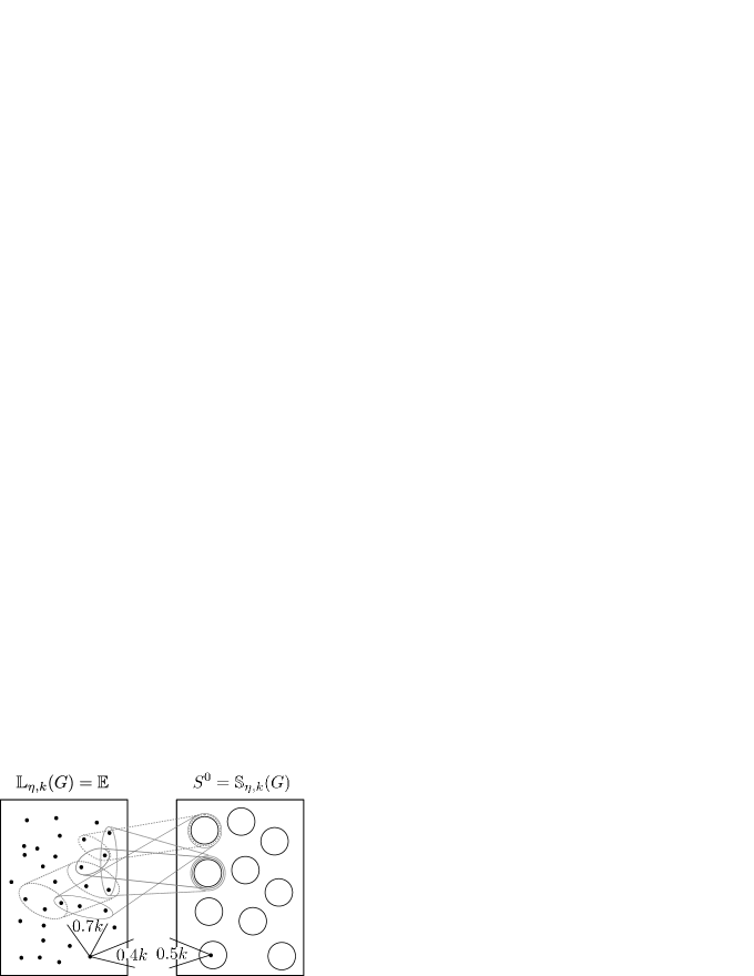
Figure 5.2 shows a graph with . Let us describe the construction of such a graph . We partition the vertex sets into to-be sets and . We further gather vertices of into clusters. We now insert edges into . All the edges inserted will be in the form of dense spots. These dense spots have either both parts in , or one part and the other in . We do this so that each inserted dense spot in the -part respects the cluster structure, while it behaves in a random-like way in the -part. Further, we require that each -vertex sends edges to and edges to , and each -vertex receives edges from . Clearly, such a construction is possible.
The point of the construction is that , and that form clusters which do not induce any dense regular pairs. No vertex has degree outside , and the cluster graph contains no matching.
However, in this situation we can still find a large regularized matching between and , by regularizing the crossing dense spots (which we can assume to be the original dense spots inserted in our construction). In general, obtaining a regularized matching is, of course, more complicated. Given the above example, one may ask whether the graph has any role at all. The answer is that for constructing , we can either use directly the edges of , or, if we do not have these edges the information about their lack helps us to find elsewhere.
5.3 Finding the structure
We can now state the main result of this paper.
Lemma 5.4.
For every , there is a number so that for every there exist such that for every there exists a number such that for every with , every with and every with the following holds.
Suppose is a -sparse decomposition of a graph with respect to and which captures all but at most edges of . Let be the size of the clusters .777The number is irrelevant when . In particular, note that in that case we necessarily have for the regularized matchings given by the lemma. Write
| (5.6) |
Then contains two -regularized matchings and such that for the triple we have
-
(a)
,
-
(b)
,
-
(c)
for each , there is a dense spot with , , and furthermore, either or , and or ,
-
(d)
for each there exists a cluster such that , and for each we have or there exists such that ,
-
(e)
,
-
(f)
,
-
(g)
for the regularized matching we have ,
-
(h)
for we have that each -edge is an edge of , and at least one of the following conditions holds
-
(K1)
,
-
(K2)
.
-
(K1)
Remark 5.5.
As explained in Section 5.1, property (h) is the most important part of Lemma 5.4. Note that the assertion (K2) implies a quantitatively weaker version of (K1). Indeed, consider . An average vertex sends at least edges to . Thus, if then induces at least edges in . Such a bound, however, would be insufficient for our purposes as later . So, the deficit in the number of edges asserted in (K2) (compared to the part of (K1)) is compensated by the fact that these edges are already regularized.
For the proof we need the well-known Gallai–Edmonds Matching Theorem, which we state next. A graph is called factor-criticalfactor-critical if has a perfect matching for each .
Theorem 5.6 (Gallai–Edmonds matching theorem (see for instance [Die05, Theorem 2.2.3])).
Let be a graph. Then there exist a set and a matching of size in such that
-
(1)
every component of is factor-critical, and
-
(2)
matches every vertex in to a different component of .
The set in Theorem 5.6 is often referred to as a separatorseparator.
Proof of Lemma 5.4.
The idea of the proof is to first obtain some information about the structure of the graph with the help of Theorem 5.6. Then the structure given by Theorem 5.6 is refined by Lemma 4.8 to yield the assertions of the lemma.
Let us begin with setting the parameters. Let be given by Lemma 4.8 for input parameters , , and let and be given by Lemma 4.8 for further input parameter . Last, let be given by Lemma 4.8 with the above parameters and .
Without loss of generality we assume that and . We write and . Further, let .
Let be a separator and let be a matching given by Theorem 5.6 applied to the graph . We will presume that the pair is chosen among all the possible choices so that the number of vertices of that are isolated in and are not covered by is minimized. Let denote the set of vertices in that are isolated in . Recall that the components of are factor-critical.
Define as a minimal set such that
-
•
, and
-
•
if and there is an edge with , , then .
Then each vertex from is reachable from by a path in that alternates between and , and has every second edge in . Also note that for all with and we have
| (5.7) |
Let us prove another property of .
Claim 5.5.1.
. In particular, .
Proof of Claim 5.5.1.
By the definition of , we only need to show that . So suppose there is a vertex . By the definition of there is a non-trivial path going from to that alternates between and , and has every second edge in . Then, the matching covers more vertices of than does. Further, it is straightforward to check that the separator together with the matching satisfies the assertions of Theorem 5.6. This is a contradiction, as desired. ∎
Using a very similar alternating path argument we see the following.
Claim 5.5.2.
If with and then .
Using the factor-criticality of the components of we extend to a matching as follows. For each component of which meets , we add a perfect matching of . Furthermore, for each non-singleton component of which does not meet , we add a matching which meets all but exactly one vertex of . This is possible as by the definition of the class we have that is edgeless, and so . This choice of guarantees that
| (5.8) |
We set
We have that
| (5.9) |
As is an independent set in , we have that
| (5.10) |
The matching in corresponds to an -regularized matching in the underlying graph , with (recall that regularized matchings have orientations on their edges). Likewise, we define as the -regularized matching corresponding to . The -edges are oriented so that ; this condition does not specify orientations of all the -edges and we orient the remaining ones in an arbitrary fashion. We write .
Claim 5.5.3.
.
Proof of Claim 5.5.3.
We prepare ourselves for an application of Lemma 4.8. The numerical parameters of the lemma are and as above. The input objects for the lemma are the graph of order , the collection of -dense spots , the matching , the -ensemble , and the set . Note that Definition 3.4, item 6, implies that absorbs . Further, (4.20) is satisfied by Definition 3.4, item 7.
The output of Lemma 4.8 is an -regularized matching with the following properties.
-
(I)
.
-
(II)
For each there are sets and such that and either or there exists such that .
(Indeed, to see this we use that and that by the definition of .)
-
(III)
There is a partition of into and such that
We claim that also
-
(IV)
.
Indeed, let be arbitrary. Then by (II) there is such that . By Claim 5.5.1, is a singleton component of . In particular, if is covered by then . It follows that . In a similar spirit, the easy fact that together with (II) gives . This establishes (IV).
Set
| (5.13) |
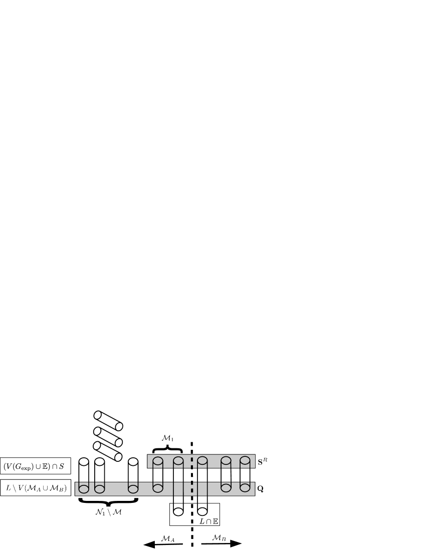
Then is an -regularized matching. Note that from now on, the sets and are defined. The situtation is illustrated in Figure 5.3.
By (IV), we have , as required for Lemma 5.4(a). Lemma 5.4(b) follows from (5.12). The claim below asserts that the next two properties are satisfied as well.
Proof of Claim 5.5.4.
Consider an arbitrary pair . Either we have that or . In the former case, is an edge in . Then the properties for asserted in Lemma 5.4(c) and Lemma 5.4(d) follow from the fact that the cluster graph is prepartitioned with respect to and , and from Definition 3.4(6).
In the case , the asserted properties are given by (II). ∎
Claim 5.5.5.
We have .
Proof of Claim 5.5.5.
It will be convenient to work with a set , . The next two easy claims assert absence of edges of certain types incident to and .
Claim 5.5.6.
The vertices in are isolated in .
Proof of Claim 5.5.6.
Claim 5.5.7.
We have .
Proof of Claim 5.5.7.
The -inclusion of the edge-sets is clear.
Next, recall that Definition 3.6 tells us that each edge in between and is either in or in . As , the -inclusion follows. ∎
By Claim 5.5.5, we have
| (5.14) |
Claim 5.5.8.
We have
Before proving Claim 5.5.8, let us see that it implies Lemma 5.4(e). As , there are no edges between and . That means that any captured edge from to must start in or in , and must be contained in . Thus Lemma 5.4(e) follows by plugging (III) into (5.3) and into Claim 5.5.8.
Let us now turn to proving Claim 5.5.8.
Proof of Claim 5.5.8.
In order to prove (f) we first observe that
| (5.18) |
Let us turn to proving (g). First, recall that we have (cf. 5.13). Since we actually have
| (5.19) |
| (by (5.9)) | ||||
| (by (IV)) | ||||
| (5.20) |
We have
| (by (5.20)) | |||
| (by (5.18), (I)) |
as needed.
We have thus shown Lemma 5.4(a)–(g). It only remains to prove Lemma 5.4(h), which we will do in the remainder of this section.
We first collect several properties of and . The definitions of and give
| (5.21) |
Each vertex of has degree at least into , and so,
| (5.22) |
Also, for each vertex , Definition 2.3(ii) gives that
| (5.23) |
Consequently (using ),
| (5.24) | ||||
| (5.25) |
Let be defined as in Lemma 5.4(h), that is, . Note that (5.12) implies that for every . Thus by the definition of ,
| if with , then . | (5.26) |
We will now prove the first part of Lemma 5.4(h), that is, we show that each -edge is an edge of . Indeed, by (II), we have that , so as , it follows that . Thus . As corresponds to a matching in , all is as desired.
Finally, let us assume that neither (K1) nor (K2) is fulfilled. After five preliminary observations (Claim 5.5.9–Claim 5.5.13), we will derive a contradiction from this assumption.
Claim 5.5.9.
We have .
Proof of Claim 5.5.9.
To see this, recall that each -vertex is either contained in , or in . Further, if then its partner in must be in , as is independent. Now, the claim follows after noticing that . ∎
Claim 5.5.10.
We have .
Proof of Claim 5.5.10.
As , we have . Therefore,
∎
Claim 5.5.11.
We have .
Proof of Claim 5.5.11.
Claim 5.5.12.
We have .
Proof of Claim 5.5.12.
Next, we bound .
Claim 5.5.13.
We have
Proof of Claim 5.5.13.
A relatively short double counting below will lead to the final contradiction. The idea behind this computation is given in Figure 5.4.
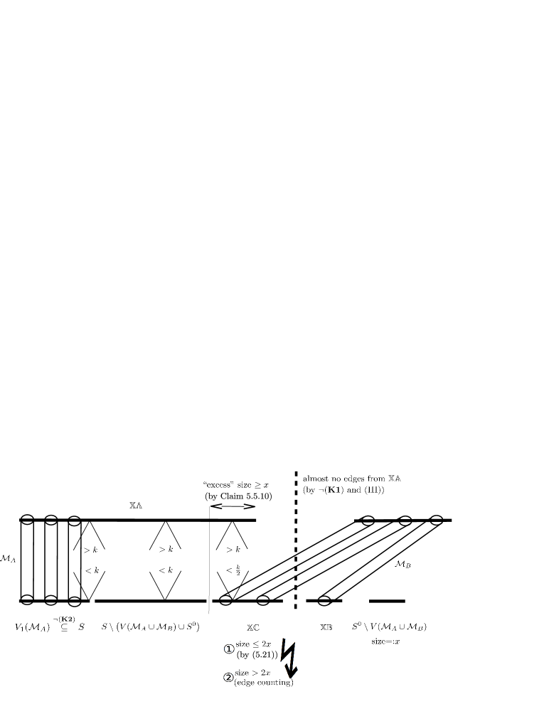
| (5.30) | ||||
a contradiction. This completes the proof of Lemma 5.4. ∎
6 Acknowledgements
The work on this project lasted from the beginning of 2008 until 2014 and we are very grateful to the following institutions and funding bodies for their support.
During the work on this paper Hladký was also affiliated with Zentrum Mathematik, TU Munich and Department of Computer Science, University of Warwick. Hladký was funded by a BAYHOST fellowship, a DAAD fellowship, Charles University grant GAUK 202-10/258009, EPSRC award EP/D063191/1, and by an EPSRC Postdoctoral Fellowship during the work on the project.
Komlós and Szemerédi acknowledge the support of NSF grant DMS-0902241.
Piguet has been also affiliated with the Institute of Theoretical Computer Science, Charles University in Prague, Zentrum Mathematik, TU Munich, the Department of Computer Science and DIMAP, University of Warwick, and the School of Mathematics, University of Birmingham. Piguet acknowledges the support of the Marie Curie fellowship FIST, DFG grant TA 309/2-1, a DAAD fellowship, Czech Ministry of Education project 1M0545, EPSRC award EP/D063191/1, and the support of the EPSRC Additional Sponsorship, with a grant reference of EP/J501414/1 which facilitated her to travel with her young child and so she could continue to collaborate closely with her coauthors on this project. This grant was also used to host Stein in Birmingham. Piguet was supported by the European Regional Development Fund (ERDF), project “NTIS — New Technologies for Information Society”, European Centre of Excellence, CZ.1.05/1.1.00/02.0090.
Stein was affiliated with the Institute of Mathematics and Statistics, University of São Paulo, the Centre for Mathematical Modeling, University of Chile and the Department of Mathematical Engineering, University of Chile. She was supported by a FAPESP fellowship, and by FAPESP travel grant PQ-EX 2008/50338-0, also CMM-Basal, FONDECYT grants 11090141 and 1140766. She also received funding by EPSRC Additional Sponsorship EP/J501414/1.
We enjoyed the hospitality of the School of Mathematics of University of Birmingham, Center for Mathematical Modeling, University of Chile, Alfréd Rényi Institute of Mathematics of the Hungarian Academy of Sciences and Charles University, Prague, during our long term visits.
The yet unpublished work of Ajtai, Komlós, Simonovits, and Szemerédi on the Erdős–Sós Conjecture was the starting point for our project, and our solution crucially relies on the methods developed for the Erdős-Sós Conjecture. Hladký, Piguet, and Stein are very grateful to the former group for explaining them those techniques.
A doctoral thesis entitled Structural graph theory submitted by Hladký in September 2012 under the supervision of Daniel Král at Charles University in Prague is based on the series of the papers [HKP+a, HKP+b, HKP+c, HKP+d]. The texts of the two works overlap greatly. We are grateful to PhD committee members Peter Keevash and Michael Krivelevich. Their valuable comments are reflected in the series.
We thank the referees for their very detailed remarks.
The contents of this publication reflects only the authors’ views and not necessarily the views of the European Commission of the European Union.
mathsymbolsSymbol index \printindexgeneralGeneral index
References
- [AKS95] M. Ajtai, J. Komlós, and E. Szemerédi. On a conjecture of Loebl. In Graph theory, combinatorics, and algorithms, Vol. 1, 2 (Kalamazoo, MI, 1992), Wiley-Intersci. Publ., pages 1135–1146. Wiley, New York, 1995.
- [Coo09] O. Cooley. Proof of the Loebl-Komlós-Sós conjecture for large, dense graphs. Discrete Math., 309(21):6190–6228, 2009.
- [Die05] R. Diestel. Graph theory, volume 173 of Graduate Texts in Mathematics. Springer-Verlag, Berlin, third edition, 2005.
- [EFLS95] P. Erdős, Z. Füredi, M. Loebl, and V. T. Sós. Discrepancy of trees. Studia Sci. Math. Hungar., 30(1-2):47–57, 1995.
- [HKP+a] J. Hladký, J. Komlós, D. Piguet, M. Simonovits, M. Stein, and E. Szemerédi. The approximate Loebl–Komlós–Sós Conjecture I: The sparse decomposition. Manuscript (arXiv:1408.3858).
- [HKP+b] J. Hladký, J. Komlós, D. Piguet, M. Simonovits, M. Stein, and E. Szemerédi. The approximate Loebl–Komlós–Sós Conjecture II: The rough structure of LKS graphs. Manuscript (arXiv:1408.3871).
- [HKP+c] J. Hladký, J. Komlós, D. Piguet, M. Simonovits, M. Stein, and E. Szemerédi. The approximate Loebl–Komlós–Sós Conjecture III: The finer structure of LKS graphs. Manuscript (arXiv:1408.3866).
- [HKP+d] J. Hladký, J. Komlós, D. Piguet, M. Simonovits, M. Stein, and E. Szemerédi. The approximate Loebl–Komlós–Sós Conjecture IV: Embedding techniques and the proof of the main result. Manuscript (arXiv:1408.3870).
- [HP15] J. Hladký and D. Piguet. Loebl–Komlós–Sós Conjecture: dense case. J. Combin. Theory Ser. B, 2015. http://dx.doi.org/10.1016/j.jctb.2015.07.004.
- [KO09] D. Kühn and D. Osthus. Embedding large subgraphs into dense graphs. In Surveys in combinatorics 2009, volume 365 of London Math. Soc. Lecture Note Ser., pages 137–167. Cambridge Univ. Press, Cambridge, 2009.
- [PS12] D. Piguet and M. J. Stein. An approximate version of the Loebl-Komlós-Sós conjecture. J. Combin. Theory Ser. B, 102(1):102–125, 2012.
- [Sze78] E. Szemerédi. Regular partitions of graphs. In Problèmes combinatoires et théorie des graphes (Colloq. Internat. CNRS, Univ. Orsay, Orsay, 1976), volume 260 of Colloq. Internat. CNRS, pages 399–401. CNRS, Paris, 1978.
- [Zha11] Y. Zhao. Proof of the conjecture for large . Electron. J. Combin., 18(1):Paper 27, 61, 2011.