The Approximate Loebl–Komlós–Sós Conjecture IV:
Embedding techniques and the proof of the main result

Abstract

This is the last paper of a series of four papers in which we prove the following relaxation of the Loebl–Komlós–Sós Conjecture: For every $\alpha>0$ there exists a number $k_{0}$ such that for every $k>k_{0}$ every $n$-vertex graph $G$ with at least $(\frac{1}{2}+\alpha)n$ vertices of degree at least $(1+\alpha)k$ contains each tree $T$ of order $k$ as a subgraph.

In the first two papers of this series, we decomposed the host graph $G$, and found a suitable combinatorial structure inside the decomposition. In the third paper, we refined this structure, and proved that any graph satisfying the conditions of the above approximate version of the Loebl–Komlós–Sós Conjecture contains one of ten specific configurations. In this paper we embed the tree $T$ in each of the ten configurations.

Mathematics Subject Classification: 05C35 (primary), 05C05 (secondary).
Keywords: extremal graph theory; Loebl–Komlós–Sós Conjecture; tree; regularity lemma; sparse graph; graph decomposition.

1 Introduction

This paper concludes a series of four papers in which we provide an approximate solution of the Loebl–Komlós–Sós Conjecture. The conjecture reads as follows.

Conjecture 1.1 (Loebl–Komlós–Sós Conjecture 1995 [EFLS95]).

Suppose that $G$ is an $n$-vertex graph with at least $n/2$ vertices of degree more than $k-2$. Then $G$ contains each tree of order $k$.

We discuss the history and state of the art in detail in the first paper [HKP⁺a] of our series. Our main result, which we prove in the present paper, is the approximate solution of the Loebl–Komlós–Sós Conjecture, and reads as follows.

Theorem 1.2 (Main result).

For every $\alpha>0$ there exists a number $k_{0}$ such that for any $k>k_{0}$ we have the following. Each $n$-vertex graph $G$ with at least $(\frac{1}{2}+\alpha)n$ vertices of degree at least $(1+\alpha)k$ contains each tree $T$ of order $k$.

In the first paper [HKP⁺a] of the series we exposed a decomposition technique (the sparse decomposition), and in the second paper [HKP⁺b], we found a rough combinatorial structure in the host graph $G$. In [HKP⁺c], the third paper of the series, we refined this structure, and obtained one of ten possible configurations, at least one of which appears in any graph satisfying the hypotheses of Theorem 1.2. These configurations will be reintroduced in Section 5. All the configurations are built up from basic elements which are inherited from the sparse decomposition.

In the present paper, we will embed the tree $T$ in the host graph $G$ using the preprocessing from [HKP⁺c]. Let us give a short outline of this procedure. First, we cut the tree into smaller subtrees, connected by few vertices. This will be done in Section 3.

We then develop techniques to embed the smaller subtrees in different building blocks of the configurations. Then, for each of the configurations, we show how to combine the embedding techniques for smaller trees to embed the whole tree $T$. All of this will be done in Section 6. We mention that Section 6.1 contains a 5-page overview of the embedding procedures, with all the relevant ideas.

Finally, in Section 7, we prove Theorem 1.2, with the help of the main results from the earlier papers [HKP⁺a, HKP⁺b, HKP⁺c].

2 Notation and preliminaries

2.1 General notation

The set $\{1,2,\ldots,n\}$ of the first $n$ positive integers is denoted by *@$[n]$$[n]$. We frequently employ indexing by many indices. We write superscript indices in parentheses (such as $a^{(3)}$), as opposed to notation of powers (such as $a^{3}$). We sometimes use subscript to refer to parameters appearing in a fact/lemma/theorem. For example $\alpha_{\mathrm{T}\ref{thm:main}}$ refers to the parameter $\alpha$ from Theorem 1.2. We omit rounding symbols when this does not lead to confusion.

We use lower case Greek letters to denote small positive constants. The exception is the letter $\phi$ which is reserved for embedding of a tree $T$ in a graph $G$, $\phi:V(T)\rightarrow V(G)$. The capital Greek letters are used for large constants.

We write *VG@$V(G)$$V(G)$ and *EG@$E(G)$$E(G)$ for the vertex set and edge set of a graph $G$, respectively. Further, *VG@$v(G)$$v(G)=|V(G)|$ is the order of $G$, and *EG@$e(G)$$e(G)=|E(G)|$ is its number of edges. If $X,Y\subseteq V(G)$ are two not necessarily disjoint sets of vertices we write *EX@$e(X)$$e(X)$ for the number of edges induced by $X$, and *EXY@$e(X,Y)$$e(X,Y)$ for the number of ordered pairs $(x,y)\in X\times Y$ for which $xy\in E(G)$. In particular, note that $2e(X)=e(X,X)$.

*DEG@$\deg$*MINDEG@$\mathrm{mindeg}$*MAXDEG@$\mathrm{maxdeg}$ For a graph $G$, a vertex $v\in V(G)$ and a set $U\subseteq V(G)$, we write $\deg(v)$ and $\deg(v,U)$ for the degree of $v$, and for the number of neighbours of $v$ in $U$, respectively. We write $\mathrm{mindeg}(G)$ for the minimum degree of $G$, $\mathrm{mindeg}(U):=\min\{\deg(u)\>:\>u\in U\}$, and $\mathrm{mindeg}(V_{1},V_{2})=\min\{\deg(u,V_{2})\>:\>u\in V_{1}\}$ for two sets $V_{1},V_{2}\subseteq V(G)$. Similar notation is used for the maximum degree, denoted by $\mathrm{maxdeg}(G)$. The neighbourhood of a vertex $v$ is denoted by *N@$\mathrm{N}(v)$$\mathrm{N}(v)$. We set $\mathrm{N}(U):=\bigcup_{u\in U}\mathrm{N}(u)$. The symbol $-$ is used for two graph operations: if $U\subseteq V(G)$ is a vertex set then $G-U$ is the subgraph of $G$ induced by the set $V(G)\setminus U$. If $H\subseteq G$ is a subgraph of $G$ then the graph $G-H$ is defined on the vertex set $V(G)$ and corresponds to deletion of edges of $H$ from $G$.

2.2 Regular pairs

In this section we introduce the notion of regular pairs which is central for Szemerédi’s regularity lemma. We also list some simple properties of regular pairs that will be useful in our embedding process.

Given a graph $H$ and two disjoint sets $U,W\subseteq V(H)$ the density*D@$\mathrm{d}(U,W)$density of the pair $(U,W)$ is defined as

$$\mathrm{d}(U,W):=\frac{e(U,W)}{|U||W|}\;.$$

Similarly, for a bipartite graph $G$ with colour classes $U$, $W$ we talk about its bipartite densitybipartite density*D@$\mathrm{d}(G)$ $\mathrm{d}(G)=\frac{e(G)}{|U||W|}$. For a given $\varepsilon>0$, a pair $(U,W)$ of disjoint sets $U,W\subseteq V(H)$ is called an regular pair$\varepsilon$-regular pair if $|\mathrm{d}(U,W)-\mathrm{d}(U^{\prime},W^{\prime})|<\varepsilon$ for every $U^{\prime}\subseteq U$, $W^{\prime}\subseteq W$ with $|U^{\prime}|\geqslant\varepsilon|U|$, $|W^{\prime}|\geqslant\varepsilon|W|$. If the pair $(U,W)$ is not $\varepsilon$-regular, then we call it irregular$\varepsilon$-irregular. A stronger notion than regularity is that of super-regularity which we recall now. A pair $(A,B)$ is super-regular pair$(\varepsilon,\gamma)$-super-regular if it is $\varepsilon$-regular, $\mathrm{mindeg}(A,B)\geqslant\gamma|B|$, and $\mathrm{mindeg}(B,A)\geqslant\gamma|A|$. Note that then $(A,B)$ has bipartite density at least $\gamma$.

The following two well-known properties of regular pairs will be useful.

Fact 2.1.

Suppose that $(U,W)$ is an $\varepsilon$-regular pair of density $d$. Let $U^{\prime}\subseteq U$ and $W^{\prime}\subseteq W$ be sets of vertices with $|U^{\prime}|\geqslant\alpha|U|$ and $|W^{\prime}|\geqslant\alpha|W|$, where $\alpha>\varepsilon$. Then the pair $(U^{\prime},W^{\prime})$ is a $2\varepsilon/\alpha$-regular pair of density at least $d-\varepsilon$.

Fact 2.2.

Suppose that $(U,W)$ is an $\varepsilon$-regular pair of density $d$. Then all but at most $\varepsilon|U|$ vertices $v\in U$ satisfy $\deg(v,W)\geqslant(d-\varepsilon)|W|$.

2.3 LKS graphs

*LKSgraphs@$\mathbf{LKS}({n},{k},{\eta})$

Write *LKSgraphs@$\mathbf{LKS}({n},{k},{\eta})$$\mathbf{LKS}({n},{k},{\alpha})$ for the class of all $n$-vertex graphs with at least $(\frac{1}{2}+\alpha)n$ vertices of degrees at least $(1+\alpha)k$. Write *Trees@$\mathbf{trees}({m})$$\mathbf{trees}({m})$ for the class of all trees on $m$ vertices. With this notation, Conjecture 1.1 states that every graph in $\mathbf{LKS}({n},{k},{0})$ contains every tree from $\mathbf{trees}({k+1})$.

Define *LKSmingraphs@$\mathbf{LKSmin}({n},{k},{\eta})$ $\mathbf{LKSmin}({n},{k},{\eta})$ as the set of all graphs $G\in\mathbf{LKS}({n},{k},{\eta})$ that are edge-minimal in $\mathbf{LKS}({n},{k},{\eta})$. Write *S@$\mathbb{S}_{{\eta},{k}}({G})$$\mathbb{S}_{{\eta},{k}}({G})$ for the set of all vertices of $G$ that have degree less than $(1+\eta)k$, and set *L@$\mathbb{L}_{{\eta},{k}}({G})$$\mathbb{L}_{{\eta},{k}}({G}):=V(G)\setminus\mathbb{S}_{{\eta},{k}}({G})$.

Definition 2.3.

Let *LKSsmallgraphs@$\mathbf{LKSsmall}({n},{k},{\eta})$$\mathbf{LKSsmall}({n},{k},{\eta})$ be the class of those graphs $G\in\mathbf{LKS}({n},{k},{\eta})$ for which we have the following three properties:

1. All the neighbours of every vertex $v\in V(G)$ with $\deg(v)>\lceil(1+2\eta)k\rceil$ have degrees at most $\lceil(1+2\eta)k\rceil$.

2. All the neighbours of every vertex of $\mathbb{S}_{{\eta},{k}}({G})$ have degree exactly $\lceil(1+\eta)k\rceil$.

3. We have $e(G)\leqslant kn$.

3 Trees

In this section we will show how to partition any given tree into small subtrees, connected by only a few vertices; this is what we call an $\ell$-fine partition. This notion is essential for our proof of Theorem 1.2, as we can embed these small subtrees one at a time.

Similar but simpler tree-cutting procedures were used earlier for the dense case of the Loebl–Komlós–Sós Conjecture [AKS95, HP16, PS12, Zha11]. There, the small trees were embedded in regular pairs of a regularity lemma decomposition of the host graph $G$. Since here, we use the sparse decomposition instead, we had to take more care when cutting the tree. (In particular, features (h), (i), (j) of Definition 3.3 are needed for the more complex setting here.)

If $T$ is a tree and $r\in V(T)$, then the pair $(T,r)$ is a rooted treerooted tree with root $r$. We write *Veven@$V_{\mathrm{even}}(T,r)$*Vodd@$V_{\mathrm{odd}}(T,r)$$V_{\mathrm{odd}}(T,r)\subseteq V(T)$ for the set of vertices of $T$ of odd distance from $r$. $V_{\mathrm{even}}(T,r)$ is defined analogously. Note that $r\in V_{\mathrm{even}}(T,r)$. The distance between two vertices $v_{1}$ and $v_{2}$ in a tree is denoted by *DIST@$\mathrm{dist}(v_{1},v_{2})$$\mathrm{dist}(v_{1},v_{2})$.

We start with a simple well-known fact about the number of leaves in a tree. For completeness we include a proof.

Fact 3.1.

Let $T$ be a tree with $\ell$ vertices of degree at least three. Then $T$ has at least $\ell+2$ leaves.

Proof.

Let $D_{1}$ be the set of leaves, $D_{2}$ the set of vertices of degree two and $D_{3}$ be the set of vertices of degree of at least three. Then

$$2(|D_{1}|+|D_{2}|+|D_{3}|)-2=2v(T)-2=2e(T)=\sum_{v\in V(T)}\deg(v)\geqslant|D_{1}|+2|D_{2}|+3|D_{3}|\;,$$

and the statement follows. ∎

Let $T$ be a tree rooted at $r$, inducing the partial order $\preceq$*@$\preceq$ on $V(T)$ (with $r$ as the minimal element). If $a\preceq b$ and $ab\in E(T)$ then we say that $b$ is a childchild of $a$ and $a$ is the parentparent of $b$. *Ch@$\mathrm{Ch}(v)$$\mathrm{Ch}(a)$ denotes the set of children of $a$, and the parent of a vertex $b\not=r$ is denoted *Par@$\mathrm{Par}(v)$$\mathrm{Par}(b)$. For a set $U\subseteq V(T)$ write *Par@$\mathrm{Par}(U)$$\mathrm{Par}(U):=\{\mathrm{Par}(u):u\in U\setminus\{r\}\}\setminus U$ and *Ch@$\mathrm{Ch}(U)$$\mathrm{Ch}(U):=\bigcup_{u\in U}\mathrm{Ch}(u)\setminus U$.

The next simple fact has already appeared in [Zha11, HP16] (and most likely in some more classic texts as well). Nevertheless, for completeness we give a proof here.

Fact 3.2.

Let $T$ be a tree with colour-classes $X$ and $Y$, and $v(T)\geqslant 2$. Then the set $X$ contains at least $|X|-|Y|+1$ leaves of $T$.

Proof.

Root $T$ at an arbitrary vertex $r\in Y$. Let $I$ be the set of internal vertices of $T$ that belong to $X$. Each $v\in I$ has at least one immediate successor in the tree order induced by $r$. These successors are distinct for distinct $v\in I$ and all lie in $Y\setminus\{r\}$. Thus $|I|\leqslant|Y|-1$. The claim follows. ∎

We say that a tree $T^{\prime}\subseteq T$ is induced treeinduced by a vertex $x\in V(T)$ if $V(T^{\prime})$ is the up-closure of $x$ in $V(T)$, i.e., $V(T^{\prime})=\{v\in V(T)\>:\>x\preceq v\}$. We then write *T@$T(r,\uparrow x)$$T^{\prime}=T(r,\uparrow x)$, or $T^{\prime}=T(\uparrow x)$, if the root is obvious from the context and call $T^{\prime}$ an end subtreeend subtree. Subtrees of $T$ that are not end subtrees are called internal subtreeinternal subtrees.

Let $T$ be a tree rooted at $r$ and let $T^{\prime}\subseteq T$ be a subtree with $r\not\in V(T^{\prime})$. The seedseed of $T^{\prime}$ is the $\preceq$-maximal vertex $x\in V(T)\setminus V(T^{\prime})$ for which $x\preceq v$ for all $v\in V(T^{\prime})$. We write *Seed@$\mathrm{Seed}$ $\mathrm{Seed}(T^{\prime})=x$. A fruitfruit in a rooted tree $(T,r)$ is any vertex $u\in V(T)$ whose distance from $r$ is even and at least four.

We can now state the most important definition of this section, that of a fine partition of a tree. The idea behind this definition is that it will be easier to embed the tree if we do it piecewise. So we partition the tree $T$ into small subtrees ($\mathcal{S}_{A}\cup\mathcal{S}_{B}$ in (a) below) of bounded size (see (e)), and a few cut-vertices (sets $W_{A}$ and $W_{B}$ in (a) below). These cut-vertices lie between the subtrees. The partition of the cut-vertices into $W_{A}$ and $W_{B}$ is inherited from the bipartition of $T$ (see (d)). The partition $\mathcal{S}_{A}$ and $\mathcal{S}_{B}$ is given by the position (in $W_{A}$ or in $W_{B}$) of the cut-vertex (i.e., seed) of the small subtree (see (f) and (g)).

It is of crucial importance that there are not too many seeds (cf. (c)), as they will have to be embedded in special sets. Namely, the set that will accommodate $W_{A}$ needs to be well connected both to the set reserved for $W_{B}$, and to the area of the graph considered for embedding the subtrees from $\mathcal{S}_{A}$. Another intuitively desirable property is (k), as the internal subtrees will be more difficult to embed than the end subtrees. This is because they are adjacent to two seeds from $W_{A}\cup W_{B}$ and after embedding (a part) of the internal subtree, we need to come back to the sets reserved for $W_{A}\cup W_{B}$ to embed the second seed.

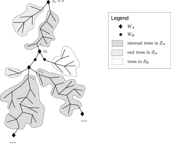
Figure 3.1: A part of an $\ell$-fine partition of a tree. Some of the properties from Definition 3.3 are illustrated. The parities obey (d) and (f). The distance between $z_{1}$ and $z_{2}$ is at least 6 as required in (i). The distance between $v_{1}$ and $v_{2}$ is more than 2 as required in (j) (since the corresponding subtrees precede one another). On the other hand, (j) does not require the distance between $v_{2}$ and $v_{3}$ to be more than 2.

Definition 3.3 ($\ell$-fine partition).

Let $T\in\mathbf{trees}({k})$ be a tree rooted at $r$. An fine partition$\ell$-fine partition of $T$ is a quadruple $(W_{A},W_{B},\mathcal{S}_{A},\mathcal{S}_{B})$, where $W_{A},W_{B}\subseteq V(T)$ and $\mathcal{S}_{A}$ and $\mathcal{S}_{B}$ are families of subtrees of $T$ such that

1. the three sets $W_{A}$, $W_{B}$ and $\{V(T^{*})\}_{T^{*}\in\mathcal{S}_{A}\cup\mathcal{S}_{B}}$ partition $V(T)$ (in particular, the trees in $T^{*}\in\mathcal{S}_{A}\cup\mathcal{S}_{B}$ are pairwise vertex disjoint),

2. $r\in W_{A}\cup W_{B}$,

3. $\max\{|W_{A}|,|W_{B}|\}\leqslant 336k/{\ell}$,

4. for $w_{1},w_{2}\in W_{A}\cup W_{B}$ the distance $\mathrm{dist}(w_{1},w_{2})$ is odd if and only if one of them lies in $W_{A}$ and the other one in $W_{B}$,

5. $v(T^{*})\leqslant\ell$ for every tree $T^{*}\in\mathcal{S}_{A}\cup\mathcal{S}_{B}$,

6. $V(T^{*})\cap\mathrm{N}(W_{B})=\emptyset$ for every $T^{*}\in\mathcal{S}_{A}$ and $V(T^{*})\cap\mathrm{N}(W_{A})=\emptyset$ for every $T^{*}\in\mathcal{S}_{B}$,

7. each tree of $\mathcal{S}_{A}\cup\mathcal{S}_{B}$ has its seeds in $W_{A}\cup W_{B}$,

8. $|\mathrm{N}(V(T^{*}))\cap(W_{A}\cup W_{B})|\leqslant 2$ for each $T^{*}\in\mathcal{S}_{A}\cup\mathcal{S}_{B}$,

9. if $\mathrm{N}(V(T^{*}))\cap(W_{A}\cup W_{B})$ contains two distinct vertices $z_{1}$ and $z_{2}$ for some $T^{*}\in\mathcal{S}_{A}\cup\mathcal{S}_{B}$, then $\mathrm{dist}_{T}(z_{1},z_{2})\geqslant 6$,

10. if $T_{1},T_{2}\in\mathcal{S}_{A}\cup\mathcal{S}_{B}$ are two internal subtrees of $T$ such that $v_{1}\in T_{1}$ precedes $v_{2}\in T_{2}$ then $\mathrm{dist}_{T}(v_{1},v_{2})>2$,

11. $\mathcal{S}_{B}$ does not contain any internal tree of $T$, and

12. $\sum_{\begin{subarray}{c}T^{*}\in\mathcal{S}_{A},\ T^{*}\textrm{end subtree of $T$}\end{subarray}}v(T^{*})\geqslant\sum_{T^{*}\in\mathcal{S}_{B}}v(T^{*})\;\mbox{.}$

An example is given in Figure 3.1.

Remark 3.4.

Suppose that $(W_{A},W_{B},\mathcal{S}_{A},\mathcal{S}_{B})$ is an $\ell$-fine partition of a tree $(T,r)$, and suppose that $T^{*}\in\mathcal{S}_{A}\cup\mathcal{S}_{B}$ is such that $|V(T^{*})\cap\mathrm{N}(W_{A}\cup W_{B})|=2$. Let us root $T^{*}$ at the neighbour $r_{1}$ of its seed, and let $r_{2}$ be the other vertex of $V(T^{*})\cap\mathrm{N}(W_{A}\cup W_{B})$. Then (d), (f), and (i) imply that $r_{2}$ is a fruit in $(T^{*},r_{1})$.

The following is the main lemma of this section.

Lemma 3.5.

Let $T\in\mathbf{trees}({k})$ be a tree rooted at $r$ and let $\ell\in[k]$. Then $T$ has an $\ell$-fine partition.

Proof.

First we shall use an inductive construction to get candidates for $W_{A}$, $W_{B}$, $\mathcal{S}_{A}$ and $\mathcal{S}_{B}$, which we shall modify later on, so that they satisfy all the conditions required by Definition 3.3.

Set $T_{0}:=T$. Now, inductively for $i\geqslant 1$ choose a $\preceq$-maximal vertex $x_{i}\in V(T_{i-1})$ with the property that $v(T_{i-1}(\uparrow x_{i}))>\ell$. We set $T_{i}:=T_{i-1}-(V(T_{i-1}(\uparrow x_{i}))\setminus\{x_{i}\})$. If, say at step $i=i_{\textrm{end}}$, no such $x_{i}$ exists, then $v(T_{i-1})\leqslant\ell$. In that case, set $x_{i}:=r$, set $W_{1}:=\{x_{i}\}_{i=1}^{i_{\textrm{end}}}$ and terminate. The fact that $v(T_{i-1}-V(T_{i}))\geqslant\ell$ for each $i<i_{\textrm{end}}$ implies that

$$|W_{1}|-1=i_{\textrm{end}}-1\leqslant k/\ell\;.$$ (3.1)

Let $\mathcal{C}$ be the set of all components of the forest $T-W_{1}$. Observe that by the choice of the $x_{i}$ each $T^{*}\in\mathcal{C}$ has order at most $\ell$.

Let $A$ and $B$ be the colour classes of $T$ such that $r\in A$. Now, choosing $W_{A}$ as $W_{1}\cap A$ and $W_{B}$ as $W_{1}\cap B$ and dividing $\mathcal{C}$ adequately into sets $\mathcal{S}_{A}$ and $\mathcal{S}_{B}$ would yield a quadruple that satisfies conditions (a), (b), (c), (d), (e) and (g). To ensure the remaining properties, we shall refine our tree partition by adding more vertices to $W_{1}$, thus making the trees in $\mathcal{S}_{A}\cup\mathcal{S}_{B}$ smaller. In doing so, we have to be careful not to end up violating (c). We shall enlarge the set of cut vertices in several steps, accomplishing sequentially, in this order, also properties (h), (j), (f), (i), and in the last step at the same time (k) and (l). It would be easy to check that during these steps none of the previously established properties is lost, so we will not explicitly check them, except for (c).

For condition (h), first define $T^{\prime}$ as the subtree of $T$ that contains all vertices of $W_{1}$ and all vertices that lie on paths in $T$ which have both endvertices in $W_{1}$. Now, if a subtree $T^{*}\in\mathcal{C}$ does not already satisfy (h) for $W_{1}$, then $V(T^{*})\cap V(T^{\prime})$ must contain some vertices of degree at least three. We will add the set $Y(T^{*})$ of all these vertices to $W_{1}$. Formally, let $Y$ be the union of the sets $Y(T^{*})$ over all $T^{*}\in\mathcal{C}$, and set $W_{2}:=W_{1}\cup Y$. Then the components of $T-W_{2}$ satisfy (h).

Let us bound the size of the set $W_{2}$. For each $T^{*}\in\mathcal{C}$, note that by Fact 3.1 for $T^{*}\cap T^{\prime}$, we know that $|Y(T^{*})|$ is at most the number of leaves of $T^{*}\cap T^{\prime}$ (minus two). On the other hand, each leaf of $T^{*}\cap T^{\prime}$ has a child in $W_{1}$ (in $T$). As these children are distinct for different trees $T^{*}\in\mathcal{C}$, we find that $|Y|\leqslant|W_{1}|$ and thus

$$|W_{2}|\leqslant 2|W_{1}|\;.$$ (3.2)

Next, for condition (j), observe that by setting $W_{3}:=W_{2}\cup\mathrm{Par}_{T}(W_{2})$ the components of $T-W_{3}$ fulfill (j). We have

$$|W_{3}|\leqslant 2|W_{2}|\overset{\eqref{Y}}{\leqslant}4|W_{1}|\;.$$ (3.3)

In order to ensure condition (f), let $R^{*}$ be the set of the roots ($\preceq$-minimal vertices) of those components $T^{*}$ of $T-W_{3}$ that contain neighbours of both colour classes of $T$. Setting $W_{4}:=W_{3}\cup R^{*}$ we see that (f) is satisfied for $W_{4}$. Furthermore, as for each vertex in $R^{*}$ there is a distinct member of $W_{3}$ above it in the order on $T$, we obtain that

$$|W_{4}|\leqslant 2|W_{3}|\overset{\eqref{eq:YY}}{\leqslant}8|W_{1}|.$$ (3.4)

Next, we shall aim for a stronger version of property (i), namely,

1. if $\mathrm{N}(V(T^{*}))\cap(W_{A}\cup W_{B})=\{z_{1},z_{2}\}$ with $z_{1}\neq z_{2}$ for some $T^{*}\in\mathcal{S}_{A}\cup\mathcal{S}_{B}$, then $\mathrm{dist}_{T}(z_{1},z_{2})\geqslant 8$.

The reason for requiring this strengthening is that later we might introduce additional cut vertices which would “shorten $T^{*}$ by two”.

Consider a component $T^{*}$ of $T-W_{4}$ which is an internal tree of $T$. If $W_{4}$ contains two distinct neighbours $z_{1}$ and $z_{2}$ of $T^{*}$ such that $\mathrm{dist}_{T}(z_{1},z_{2})<8$, then we call $T^{*}$ short. Observe that there are at most $|W_{4}|$ short trees, because each of these trees has a unique vertex from $W_{4}$ above it. Let $Z(T^{*})\subseteq V(T^{*})$ be the vertices on the path from $z_{1}$ to $z_{2}$ (excluding the end vertices). Then $|Z(T^{*})|\leqslant 7$. Letting $Z$ be the union of the sets $Z(T^{*})$ over all short trees in $T-W_{4}$, and set $W_{5}:=W_{4}\cup Z$, we obtain that

$$|W_{5}|\leqslant|W_{4}|+7|W_{4}|\overset{\eqref{W3}}{\leqslant}64|W_{1}|\overset{\eqref{X}}{\leqslant}64k/\ell+1.$$ (3.5)

We still need to ensure (k) and (l). To this end, consider the set $\mathcal{C}^{\prime}$ of all components of $T-W_{5}$. Set $\mathcal{C}^{\prime}_{A}:=\{T^{*}\in\mathcal{C}^{\prime}:\mathrm{Seed}(T^{*})\in A\}$ and set $\mathcal{C}^{\prime}_{B}:=\mathcal{C}^{\prime}\setminus\mathcal{C}^{\prime}_{A}$. We assume that

$$\sum_{T^{*}\in\mathcal{C}^{\prime}_{A}\ :\ T^{*}\textrm{ end tree of $T$}}v(T^{*})\geqslant\sum_{T^{*}\in\mathcal{C}^{\prime}_{B}\ :\ T^{*}\textrm{ end tree of $T$}}v(T^{*})\;,$$ (3.6)

as otherwise we can simply swap $A$ and $B$. Now, for each $T^{*}\in\mathcal{C}^{\prime}_{B}$ that is not an end subtree of $T$, set $X(T^{*}):=V(T^{*})\cap\mathrm{N}_{T}(W_{5})$. Let $X$ be the union of all such sets $X(T^{*})$. Observe that

$$|X|\leqslant 2|W_{5}\cap B|\leqslant 2|W_{5}|.$$ (3.7)

For $W:=W_{5}\cup X$, all internal trees of $T-W$ have their seeds in $A$. This will guarantee (k), and, together with (3.6), also (l).

Finally, set $W_{A}:=W\cap A$ and $W_{B}:=W\cap B$, and let $\mathcal{S}_{A}$ and $\mathcal{S}_{B}$ be the sets of those components of $T-W$ that have their seeds in $W_{A}$ and $W_{B}$, respectively. By construction, $(W_{A},W_{B},\mathcal{S}_{A},\mathcal{S}_{B})$ has all the properties of an $\ell$-fine partition. In particular, for (c), we find with (3.5) and (3.7) that $|W|\leqslant|W_{5}|+2|W_{5}\cap B|\leqslant 336k/\ell$. ∎

For an $\ell$-fine partition $(W_{A},W_{B},\mathcal{S}_{A},\mathcal{S}_{B})$ of a rooted tree $(T,r)$, the trees $T^{*}\in\mathcal{S}_{A}\cup\mathcal{S}_{B}$ are called shrubshrubs. An end shrub is a shrub which is an end subtree. An internal shrub is a shrub which is an internal subtree. A hubhub is a component of the forest $T[W_{A}\cup W_{B}]$. Suppose that $T^{*}\in\mathcal{S}_{A}$ is an internal shrub, and $r^{*}$ is its $\preceq_{r}$-minimal vertex. Then $T^{*}-r^{*}$ contains a unique component with a vertex from $\mathrm{N}_{T}(W_{A})$. We call this component subshrubprincipal subshrubprincipal subshrub, and the other components peripheral subshrubperipheral subshrubs.

Remark 3.6.

1. In our proof of Theorem 1.2, we shall apply Lemma 3.5 to a tree $T_{\mathrm{T}\ref{thm:main}}\in\mathbf{trees}({k})$. The number $\ell_{\mathrm{L}\ref{lem:TreePartition}}$ will be linear in $k$, and thus (c) of Definition 3.3 tells us that the size of the sets $W_{A}$ and $W_{B}$ is bounded by an absolute constant (depending on $\alpha_{\mathrm{T}\ref{thm:main}}$ only).

2. Each internal tree in $\mathcal{S}_{A}$ of an $\ell$-fine partition has a unique vertex from $W_{A}$ above it. Thus with $\ell_{\mathrm{L}\ref{lem:TreePartition}}$ as above also the number of internal trees in $\mathcal{S}_{A}$ is bounded by an absolute constant. This need not be the case for the number of end trees. For instance, if $(T_{\mathrm{T}\ref{thm:main}},r)$ is a star with $k-1$ leaves and rooted at its centre $r$ then $W_{A}=\{r\}$ while the $k-1$ leaves of $T_{\mathrm{T}\ref{thm:main}}$ form the end shrubs in $\mathcal{S}_{A}$.

Definition 3.7 (ordered skeleton).

ordered skeleton We say that the sequence $\big{(}X_{0},X_{1},\ldots,X_{m}\big{)}$ is an ordered skeleton of the $\ell$-fine partition $(W_{A},W_{B},\mathcal{S}_{A},\mathcal{S}_{B})$ of a rooted tree $(T,r)$ if

• $X_{0}$ is a hub and contains $r$, and all other $X_{i}$ are either hubs or shrubs,

• $V(\bigcup_{i\leqslant m}X_{i})=V(T)$, and

• for each $i=1,\ldots,m$, the subgraph formed by $X_{0}\cup X_{1}\cup\ldots\cup X_{i}$ is connected in $T$.

Directly from Definition 3.3 we get:

Lemma 3.8.

Any $\ell$-fine partition of any rooted tree has an ordered skeleton.

4 Necessary facts and notation from [HKP⁺a, HKP⁺b, HKP⁺c]

4.1 Sparse decomposition

We now shift our focus from preprocessing the tree to the host graph. This is where we build on results from the earlier papers in the series. We first recall the notion of dense spots and related concepts introduced in [HKP⁺a], [HKP⁺b], and [HKP⁺c].

Definition 4.1 (dense spot$(m,\gamma)$-dense spot, nowhere-dense$(m,\gamma)$-nowhere-dense).

Suppose that $m\in\mathbb{N}$ and $\gamma>0$. An $(m,\gamma)$-dense spot in a graph $G$ is a non-empty bipartite subgraph $D=(U,W;F)$ of $G$ with $\mathrm{d}(D)>\gamma$ and $\mathrm{mindeg}(D)>m$. We call $G$ $(m,\gamma)$-nowhere-dense if it does not contain any $(m,\gamma)$-dense spot.

Definition 4.2 ($(m,\gamma)$-dense cover).

dense cover Suppose that $m\in\mathbb{N}$ and $\gamma>0$. An $(m,\gamma)$-dense cover of a graph $G$ is a family $\mathcal{D}$ of edge-disjoint $(m,\gamma)$-dense spots such that $E(G)=\bigcup_{D\in\mathcal{D}}E(D)$.

The proofs of the following facts can be found in [HKP⁺b].

Fact 4.3.

Let $(U,W;F)$ be a $(\gamma k,\gamma)$-dense spot in a graph $G$ of maximum degree at most $\Omega k$. Then $\max\{|U|,|W|\}\leqslant\frac{\Omega}{\gamma}k.$

Fact 4.4.

Let $H$ be a graph of maximum degree at most $\Omega k$, let $v\in V(H)$, and let $\mathcal{D}$ be a family of edge-disjoint $(\gamma k,\gamma)$-dense spots. Then fewer than $\frac{\Omega}{\gamma}$ dense spots from $\mathcal{D}$ contain $v$.

In the following definition, note that a subset of a $(\Lambda,\varepsilon,\gamma,k)$-avoiding set is also $(\Lambda,\varepsilon,\gamma,k)$-avoiding.

Definition 4.5 (avoiding (set)$(\Lambda,\varepsilon,\gamma,k)$-avoiding set).

Suppose that $k\in\mathbb{N}$, $\varepsilon,\gamma>0$ and $\Lambda>0$. Suppose that $G$ is a graph and $\mathcal{D}$ is a family of dense spots in $G$. A set $\mathbb{E}\subseteq\bigcup_{D\in\mathcal{D}}V(D)$ is $(\Lambda,\varepsilon,\gamma,k)$-avoiding with respect to $\mathcal{D}$ if for every $U\subseteq V(G)$ with $|U|\leqslant\Lambda k$ the following holds for all but at most $\varepsilon k$ vertices $v\in\mathbb{E}$. There is a dense spot $D\in\mathcal{D}$ with $|U\cap V(D)|\leqslant\gamma^{2}k$ that contains $v$.

In the next two definitions, we expose the most important tool in the proof of our main result (Theorem 1.2): the sparse decomposition. It generalises the notion of equitable partition from Szemerédi’s regularity lemma. This is explained in [HKP⁺a, Section LABEL:p0.ssec:sparsedecompofdensegraphs]. The first step to this end is defining the bounded decomposition.

Definition 4.6 (bounded decomposition$(k,\Lambda,\gamma,\varepsilon,\nu,\rho)$-bounded decomposition).

Suppose that $k\in\mathbb{N}$ and $\varepsilon,\gamma,\nu,\rho>0$ and $\Lambda>0$. Let $\mathcal{V}=\{V_{1},V_{2},\ldots,V_{s}\}$ be a partition of the vertex set of a graph $G$. We say that $(\mathbf{V},\mathcal{D},G_{\mathrm{reg}},G_{\mathrm{exp}},\mathbb{E})$ is a $(k,\Lambda,\gamma,\varepsilon,\nu,\rho)$-bounded decomposition of $G$ with respect to $\mathcal{V}$ if the following properties are satisfied:

1. $G_{\mathrm{exp}}$ is a $(\gamma k,\gamma)$-nowhere-dense subgraph of $G$ with $\mathrm{mindeg}(G_{\mathrm{exp}})>\rho k$.

2. The elements of $\mathbf{V}$ are pairwise disjoint subsets of $V(G)$.

3. $G_{\mathrm{reg}}$ is a subgraph of $G-G_{\mathrm{exp}}$ on the vertex set $\bigcup\mathbf{V}$. For each edge $xy\in E(G_{\mathrm{reg}})$ there are distinct $C_{x}\ni x$ and $C_{y}\ni y$ from $\mathbf{V}$, and $G[C_{x},C_{y}]=G_{\mathrm{reg}}[C_{x},C_{y}]$. Furthermore, $G[C_{x},C_{y}]$ forms an $\varepsilon$-regular pair of density at least $\gamma^{2}$.

4. We have $\nu k\leqslant|C|=|C^{\prime}|\leqslant\varepsilon k$ for all $C,C^{\prime}\in\mathbf{V}$.

5. $\mathcal{D}$ is a family of edge-disjoint $(\gamma k,\gamma)$-dense spots in $G-G_{\mathrm{exp}}$. For each $D=(U,W;F)\in\mathcal{D}$ all the edges of $G[U,W]$ are covered by $\mathcal{D}$ (but not necessarily by $D$).

6. If $G_{\mathrm{reg}}$ contains at least one edge between $C_{1},C_{2}\in\mathbf{V}$, then there exists a dense spot $D=(U,W;F)\in\mathcal{D}$ such that $C_{1}\subseteq U$ and $C_{2}\subseteq W$.

7. For all $C\in\mathbf{V}$ there is $V\in\mathcal{V}$ so that either $C\subseteq V\cap V(G_{\mathrm{exp}})$ or $C\subseteq V\setminus V(G_{\mathrm{exp}})$. For all $C\in\mathbf{V}$ and $D=(U,W;F)\in\mathcal{D}$ we have $C\cap U,C\cap W\in\{\emptyset,C\}$.

8. $\mathbb{E}$ is a $(\Lambda,\varepsilon,\gamma,k)$-avoiding subset of $V(G)\setminus\bigcup\mathbf{V}$ with respect to dense spots $\mathcal{D}$.

We say that the bounded decomposition $(\mathbf{V},\mathcal{D},G_{\mathrm{reg}},G_{\mathrm{exp}},\mathbb{E})$ respects the avoiding threshold $b$avoiding threshold if for each $C\in\mathbf{V}$ we either have $\mathrm{maxdeg}_{G}(C,\mathbb{E})\leqslant b$, or $\mathrm{mindeg}_{G}(C,\mathbb{E})>b$.

The members of $\mathbf{V}$ are called clusterclusters. Define the cluster graphcluster graph *Gblack@$\mathbf{G}_{\mathrm{reg}}$ $\mathbf{G}_{\mathrm{reg}}$ as the graph on the vertex set $\mathbf{V}$ that has an edge $C_{1}C_{2}$ for each pair $(C_{1},C_{2})$ which has density at least $\gamma^{2}$ in the graph $G_{\mathrm{reg}}$.

Definition 4.7 (sparse decomposition$(k,\Omega^{**},\Omega^{*},\Lambda,\gamma,\varepsilon,\nu,\rho)$-sparse decomposition).

Suppose that $k\in\mathbb{N}$ and $\varepsilon,\gamma,\nu,\rho>0$ and $\Lambda,\Omega^{*},\Omega^{**}>0$. Let $\mathcal{V}=\{V_{1},V_{2},\ldots,V_{s}\}$ be a partition of the vertex set of a graph $G$. We say that $\nabla=(\mathbb{H},\mathbf{V},\mathcal{D},G_{\mathrm{reg}},G_{\mathrm{exp}},\mathbb{E})$ is a $(k,\Omega^{**},\Omega^{*},\Lambda,\gamma,\varepsilon,\nu,\rho)$-sparse decomposition of $G$ with respect to $V_{1},V_{2},\ldots,V_{s}$ if the following holds.

1. $\mathbb{H}\subseteq V(G)$, $\mathrm{mindeg}_{G}(\mathbb{H})\geqslant\Omega^{**}k$, $\mathrm{maxdeg}_{H}(V(G)\setminus\mathbb{H})\leqslant\Omega^{*}k$, where $H$ is spanned by the edges of $\bigcup\mathcal{D}$, $G_{\mathrm{exp}}$, and edges incident with $\mathbb{H}$,

2. $(\mathbf{V},\mathcal{D},G_{\mathrm{reg}},G_{\mathrm{exp}},\mathbb{E})$ is a $(k,\Lambda,\gamma,\varepsilon,\nu,\rho)$-bounded decomposition of $G-\mathbb{H}$ with respect to $V_{1}\setminus\mathbb{H},V_{2}\setminus\mathbb{H},\ldots,V_{s}\setminus\mathbb{H}$.

If the parameters do not matter, we call $\nabla$ simply a sparse decomposition, and similarly we speak about a bounded decomposition. We define the graph *GD@$G_{\mathcal{D}}$$G_{\mathcal{D}}$ as the union (both edge-wise, and vertex-wise) of all dense spots $\mathcal{D}$.

Fact 4.8 ([HKP⁺a, Fact LABEL:p0.fact:clustersSeenByAvertex]).

Let $\nabla=(\mathbb{H},\mathbf{V},\mathcal{D},G_{\mathrm{reg}},G_{\mathrm{exp}},\mathbb{E})$ be a $(k,\Omega^{**},\Omega^{*},\Lambda,\gamma,\varepsilon,\nu,\rho)$-sparse decomposition of a graph $G$. Let $x\in V(G)\setminus\mathbb{H}$. Assume that $\mathbf{V}\not=\emptyset$, and let $\mathfrak{c}$ be the size of each of the members of $\mathbf{V}$. Then there are fewer than

$$\frac{2(\Omega^{*})^{2}k}{\gamma^{2}\mathfrak{c}}\leqslant\frac{2(\Omega^{*})^{2}}{\gamma^{2}\nu}$$

clusters $C\in\mathbf{V}$ with $\deg_{G_{\mathcal{D}}}(x,C)>0$.

Definition 4.9 (captured edgescaptured edges).

In the situation of Definition 4.7, we refer to the edges in $E(G_{\mathrm{reg}})\cup E(G_{\mathrm{exp}})\cup E_{G}(\mathbb{H},V(G))\cup E_{G_{\mathcal{D}}}(\mathbb{E},\mathbb{E}\cup\bigcup\mathbf{V})$ as captured edgescaptured by the sparse decomposition. Denote by *Gclass@$G_{\nabla}$$G_{\nabla}$ the spanning subgraph of $G$ whose edges are the captured edges of the sparse decomposition. Likewise, the captured edges of a bounded decomposition $(\mathbf{V},\mathcal{D},G_{\mathrm{reg}},G_{\mathrm{exp}},\mathbb{E})$ of a graph $G$ are those in $E(G_{\mathrm{reg}})\cup E(G_{\mathrm{exp}})\cup E_{G_{\mathcal{D}}}(\mathbb{E},\mathbb{E}\cup\bigcup\mathbf{V})$.

The last definition we need is the notion of a regularized matching.

Definition 4.10 ($(\varepsilon,d,\ell)$-regularized matching).

Suppose that $\ell\in\mathbb{N}$ and $d,\varepsilon>0$. A collection $\mathcal{N}$ of pairs $(A,B)$ with $A,B\subseteq V(H)$ is called an regularized@regularized matching$(\varepsilon,d,\ell)$-regularized matching of a graph $H$ if

1. $|A|=|B|\geqslant\ell$ for each $(A,B)\in\mathcal{N}$,

2. $(A,B)$ induces in $H$ an $\varepsilon$-regular pair of density at least $d$, for each $(A,B)\in\mathcal{N}$, and

3. all involved sets $A$ and $B$ are pairwise disjoint.

Sometimes, when the parameters do not matter we simply write regularized matching.

We say that a regularized matching $\mathcal{N}$ absorbabsorbes a regularized matching $\mathcal{M}$ if for every $(S,T)\in\mathcal{M}$ there exists $(X,Y)\in\mathcal{N}$ such that $S\subseteq X$ and $T\subseteq Y$. In the same way, we say that a family of dense spots $\mathcal{D}$ absorbabsorbes a regularized matching $\mathcal{M}$ if for every $(S,T)\in\mathcal{M}$ there exists $(U,W;F)\in\mathcal{D}$ such that $S\subseteq U$ and $T\subseteq W$.

Fact 4.11 ([HKP⁺b, Fact LABEL:p1.fact:boundMatchingClusters]).

Suppose that $\mathcal{M}$ is an $(\varepsilon,d,\ell)$-regularized matching in a graph $H$. Then $|C|\leqslant\frac{\mathrm{maxdeg}{(H)}}{d}$ for each $C\in\mathcal{V}(\mathcal{M})$.

4.2 Shadows

We recall the notion of a shadow given in [HKP⁺c]. Given a graph $H$, a set $U\subseteq V(H)$, and a number $\ell$ we define inductively *SHADOW@$\mathrm{shadow}(U,\ell)$shadow

$$\mathrm{shadow}^{(0)}_{H}(U,\ell):=U\text{, and }$$

$$\mathrm{shadow}^{(i)}_{H}(U,\ell):=\{v\in V(H)\>:\>\deg_{H}(v,\mathrm{shadow}^{(i-1)}_{H}(U,\ell))>\ell\}\text{ for }i\geqslant 1.$$

exponent of shadowWe call the index $i$ the exponent of the shadow. We abbreviate $\mathrm{shadow}^{(1)}_{H}(U,\ell)$ as $\mathrm{shadow}_{H}(U,\ell)$. Further, the graph $H$ is omitted from the subscript if it is clear from the context. Note that the shadow of a set $U$ might intersect $U$.

The proofs of the following facts can be found in [HKP⁺c].

Fact 4.12.

Suppose $H$ is a graph with $\mathrm{maxdeg}(H)\leqslant\Omega k$. Then for each $\alpha>0,i\in\{0,1,\ldots\}$, and each set $U\subseteq V(H)$, we have

$$|\mathrm{shadow}^{(i)}(U,\alpha k)|\leqslant\left(\frac{\Omega}{\alpha}\right)^{i}|U|\;.$$

Fact 4.13.

Let $\alpha,\gamma,Q>0$ be three numbers such that $1\leqslant Q\leqslant\frac{\alpha}{16\gamma}$. Suppose that $H$ is a $(\gamma k,\gamma)$-nowhere-dense graph, and let $U\subseteq V(H)$ with $|U|\leqslant Qk$. Then we have

$$|\mathrm{shadow}(U,\alpha k)|\leqslant\frac{16Q^{2}\gamma}{\alpha}k.$$

5 Configurations

5.1 Common settings

Recall the definitions of $\mathbb{S}_{{\eta},{k}}({G})$ and $\mathbb{L}_{{\eta},{k}}({G})$ given in Section 2.3. We repeat some common settings that already appeared in [HKP⁺c] and are outputs of [HKP⁺b, Lemma LABEL:p1.prop:LKSstruct]. The reader can find explanations in [HKP⁺b, Section LABEL:p1.ssec:motivation] why the set $\mathbb{XA}$ (defined again in (5.3)) has excellent properties for accommodating cut-vertices of $T_{\mathrm{T}\ref{thm:main}}$, and the set $\mathbb{XB}$ has “half-that-excellent properties” for accommodating cut-vertices. In particular, the formula defining $\mathbb{XB}$ suggests that we cannot make use of the set $\mathbb{S}_{{\eta},{k}}({G})\setminus(V(G_{\mathrm{exp}})\cup\mathbb{E}\cup V(\mathcal{M}_{A}\cup\mathcal{M}_{B})$ for the purpose of embedding shrubs neighbouring the cut-vertices embedded in $\mathbb{XB}$. In [HKP⁺c, Setting LABEL:p2.commonsetting] we gave some motivation behind the definition of the sets $V_{+},L_{\#},V_{\mathrm{good}},\mathbb{YA},\mathbb{YB},V_{\leadsto\mathbb{H}},\mathbb{J}_{\mathbb{E}},\mathbb{J},\mathbb{J}_{1},\mathbb{J}_{2},\mathbb{J}_{3}$, and $\mathcal{F}$ in Setting 5.1, below.

Setting 5.1.

We assume that the constants $\Lambda,\Omega^{*},\Omega^{**},k_{0}$ and $\widehat{\alpha},\gamma,\varepsilon,\varepsilon^{\prime},\eta,\pi,\rho,\tau,d$ satisfy

$$\begin{split}\eta\gg\frac{1}{\Omega^{*}}\gg\frac{1}{\Omega^{**}}\gg\rho\gg\gamma\gg d\geqslant\frac{1}{\Lambda}\geqslant\varepsilon\geqslant\pi\geqslant\widehat{\alpha}\geqslant\varepsilon^{\prime}\geqslant\nu\gg\tau\gg\frac{1}{k_{0}}>0\;,\end{split}$$ (5.1)

and that $k\geqslant k_{0}$. By writing $c>a_{1}\gg a_{2}\gg\ldots\gg a_{\ell}>0$ we mean that there exist suitable non-decreasing functions $f_{i}:(0,c)^{i}\rightarrow(0,c)$ ($i=1,\ldots,\ell-1$) such that for each $i\in[\ell-1]$ we have $a_{i+1}<f_{i}(a_{1},\ldots,a_{i})$. A suitable choice of these functions in (5.1) is explicitly given in Section 7.

Suppose that $G\in\mathbf{LKSsmall}({n},{k},{\eta})$ is given together with its $(k,\Omega^{**},\Omega^{*},\Lambda,\gamma,\varepsilon^{\prime},\nu,\rho)$-sparse decomposition *@$\nabla$

$$\nabla=(\mathbb{H},\mathbf{V},\mathcal{D},G_{\mathrm{reg}},G_{\mathrm{exp}},\mathbb{E})\;,$$

with respect to the partition $\{\mathbb{S}_{{\eta},{k}}({G}),\mathbb{L}_{{\eta},{k}}({G})\}$, and with respect to the avoiding threshold $\frac{\rho k}{100\Omega^{*}}$. We write

$${*VA@V_{\leadsto\mathbb{E}}}{*VA@\mathbf{V}_{\leadsto\mathbb{E}}}V_{\leadsto\mathbb{E}}:=\mathrm{shadow}_{G_{\nabla}-\mathbb{H}}(\mathbb{E},\frac{\rho k}{100\Omega^{*}})\quad\mbox{and}\quad\mathbf{V}_{\leadsto\mathbb{E}}:=\{C\in\mathbf{V}\>:\>C\subseteq V_{\leadsto\mathbb{E}}\}\;.$$ (5.2)

The graph *Gblack@$\mathbf{G}_{\mathrm{reg}}$$\mathbf{G}_{\mathrm{reg}}$ is the corresponding cluster graph. Let $\mathfrak{c}$ *C@$\mathfrak{c}$ be the size of an arbitrary cluster in $\mathbf{V}$. Let *G@$G_{\nabla}$$G_{\nabla}$ be the spanning subgraph of $G$ formed by the edges captured by the sparse decomposition $\nabla$. There are two $(\varepsilon,d,\pi\mathfrak{c})$-regularized matchings $\mathcal{M}_{A}$ and $\mathcal{M}_{B}$ in $G_{\mathcal{D}}$, with the following properties. Following [HKP⁺b, (LABEL:p1.def:XAXBXC)] we write

$$\begin{split}\mathbb{XA}&:=\mathbb{L}_{{\eta},{k}}({G})\setminus V(\mathcal{M}_{B})\;,\\ \mathbb{XB}&:=\left\{v\in V(\mathcal{M}_{B})\cap\mathbb{L}_{{\eta},{k}}({G})\>:\>\widehat{\deg}(v)<(1+\eta)\frac{k}{2}\right\}\;,\\ \mathbb{XC}&:=\mathbb{L}_{{\eta},{k}}({G})\setminus(\mathbb{XA}\cup\mathbb{XB})\;,\end{split}$$ (5.3)

where $\widehat{\deg}(v)$ on the second line is defined by

$$\widehat{\deg}(v):=\deg_{G}\big{(}v,\mathbb{S}_{{\eta},{k}}({G})\setminus(V(G_{\mathrm{exp}})\cup\mathbb{E}\cup V(\mathcal{M}_{A}\cup\mathcal{M}_{B})\big{)}\;.$$

Then we have

1. $V(\mathcal{M}_{A})\cap V(\mathcal{M}_{B})=\emptyset$,

2. $V_{1}(\mathcal{\mathcal{M}}_{B})\subseteq S^{0}$, where

   $$S^{0}:=\mathbb{S}_{{\eta},{k}}({G})\setminus(V(G_{\mathrm{exp}})\cup\mathbb{E})\;,$$ (5.4)

3. for each $(X,Y)\in\mathcal{M}_{A}\cup\mathcal{M}_{B}$, there is a dense spot $(U,W;F)\in\mathcal{D}$ with $X\subseteq U$ and $Y\subseteq W$, and further, either $X\subseteq\mathbb{S}_{{\eta},{k}}({G})$ or $X\subseteq\mathbb{L}_{{\eta},{k}}({G})$, and $Y\subseteq\mathbb{S}_{{\eta},{k}}({G})$ or $Y\subseteq\mathbb{L}_{{\eta},{k}}({G})$,

4. for each $X_{1}\in\mathcal{V}_{1}(\mathcal{M}_{A}\cup\mathcal{M}_{B})$ there exists a cluster $C_{1}\in\mathbf{V}$ such that $X_{1}\subseteq C_{1}$, and for each $X_{2}\in\mathcal{V}_{2}(\mathcal{M}_{A}\cup\mathcal{M}_{B})$ there exists $C_{2}\in\mathbf{V}\cup\{\mathbb{L}_{{\eta},{k}}({G})\cap\mathbb{E}\}$ such that $X_{2}\subseteq C_{2}$,

5. each pair of the regularized matching $\mathcal{M}_{\mathrm{good}}:=\{(X_{1},X_{2})\in\mathcal{M}_{A}\>:\>X_{1}\cup X_{2}\subseteq\mathbb{XA}\}$ corresponds to an edge in $\mathbf{G}_{\mathrm{reg}}$,

6. $e_{G_{\nabla}}\big{(}\mathbb{XA},S^{0}\setminus V(\mathcal{M}_{A})\big{)}\leqslant\gamma kn$,

7. $e_{G_{\mathrm{reg}}}(V(G)\setminus V(\mathcal{M}_{A}\cup\mathcal{M}_{B}))\leqslant\gamma^{2}kn$,

8. for the regularized matching *Natom@${\mathcal{N}_{\mathbb{E}}}$ ${\mathcal{N}_{\mathbb{E}}}:=\{(X,Y)\in\mathcal{M}_{A}\cup\mathcal{M}_{B}\>:\>(X\cup Y)\cap\mathbb{E}\not=\emptyset\}$ we have $e_{G_{\mathrm{reg}}}\big{(}V(G)\setminus V(\mathcal{M}_{A}\cup\mathcal{M}_{B}),V({\mathcal{N}_{\mathbb{E}}})\big{)}\leqslant\gamma^{2}kn$,

9. $|E(G)\setminus E(G_{\nabla})|\leqslant 2\rho kn$,

10. $|E(G_{\mathcal{D}})\setminus(E(G_{\mathrm{reg}})\cup E_{G}[\mathbb{E},\mathbb{E}\cup\bigcup\mathbf{V}])|\leqslant\frac{5}{4}\gamma kn$.

We write

$${*V_{+}@$V_{+}$}V_{+} :=V(G)\setminus(S^{0}\setminus V(\mathcal{M}_{A}\cup\mathcal{M}_{B}))$$ (5.5)

$$=\mathbb{L}_{{\eta},{k}}({G})\cup V(G_{\mathrm{exp}})\cup\mathbb{E}\cup V(\mathcal{M}_{A}\cup\mathcal{M}_{B})\;,$$ (5.6)

$${*L@$L_{\#}$}L_{\#} :=\mathbb{L}_{{\eta},{k}}({G})\setminus\mathbb{L}_{{\frac{9}{10}\eta},{k}}({G_{\nabla}})\;\mbox{, and}$$ (5.7)

$${*Vgood@$V_{\mathrm{good}}$}V_{\mathrm{good}} :=V_{+}\setminus(\mathbb{H}\cup L_{\#})\;,$$ (5.8)

$$\mathbb{YA} :=\mathrm{shadow}_{G_{\nabla}}\left(V_{+}\setminus L_{\#},(1+\frac{\eta}{10})k\right)\setminus\mathrm{shadow}_{G-G_{\nabla}}\left(V(G),\frac{\eta}{100}k\right)\;,{*YA@$\mathbb{YA}$}$$ (5.9)

$$\mathbb{YB} :=\mathrm{shadow}_{G_{\nabla}}\left(V_{+}\setminus L_{\#},(1+\frac{\eta}{10})\frac{k}{2}\right)\setminus\mathrm{shadow}_{G-G_{\nabla}}\left(V(G),\frac{\eta}{100}k\right)\;,{*YB@$\mathbb{YB}$}$$ (5.10)

$$V_{\leadsto\mathbb{H}} :=(\mathbb{XA}\cup\mathbb{XB})\cap\mathrm{shadow}_{G}\left(\mathbb{H},\frac{\eta}{100}k\right){*V@$V_{\leadsto\mathbb{H}}$}\;,$$ (5.11)

$$\mathbb{J}_{\mathbb{E}} :=\mathrm{shadow}_{G_{\mathrm{reg}}}(V({\mathcal{N}_{\mathbb{E}}}),\gamma k)\setminus V(\mathcal{M}_{A}\cup\mathcal{M}_{B})\;,{*JE@$\mathbb{J}_{\mathbb{E}}$}$$

$$\mathbb{J}_{1} :=\mathrm{shadow}_{G_{\mathrm{reg}}}(V(G)\setminus V(\mathcal{M}_{A}\cup\mathcal{M}_{B}),\gamma k)\setminus V(\mathcal{M}_{A}\cup\mathcal{M}_{B})\;,{*J1@$\mathbb{J}_{1}$}$$

$$\mathbb{J} :=(\mathbb{XA}\setminus\mathbb{YA})\cup((\mathbb{XA}\cup\mathbb{XB})\setminus\mathbb{YB})\cup V_{\leadsto\mathbb{H}}\cup L_{\#}\cup\mathbb{J}_{1}$$

$$~{}~{}~{}~{}~{}\cup\mathrm{shadow}_{G_{\mathcal{D}}\cup G_{\nabla}}(V_{\leadsto\mathbb{H}}\cup L_{\#}\cup\mathbb{J}_{\mathbb{E}}\cup\mathbb{J}_{1},\frac{\eta^{2}k}{10^{5}})\;,{*J@$\mathbb{J}$}$$

$$\mathbb{J}_{2} :=\mathbb{XA}\cap\mathrm{shadow}_{G_{\nabla}}(S^{0}\setminus V(\mathcal{M}_{A}),\sqrt{\gamma}k)\;,{*J2@$\mathbb{J}_{2}$}$$

$$\mathbb{J}_{3} :=\mathbb{XA}\cap\mathrm{shadow}_{G_{\nabla}}(\mathbb{XA},\eta^{3}k/10^{3})\;,{*J3@$\mathbb{J}_{3}$}$$

$$\mathcal{F} :=\{C\in\mathcal{V}(\mathcal{M}_{A}):C\subseteq\mathbb{XA}\}\cup\mathcal{V}_{1}(\mathcal{M}_{B})\;.{*F@$\mathcal{F}$}$$ (5.12)

For the embedding procedure to run smoothly, the vertex set is split into several classes the sizes of which have given ratios. It will be important that most vertices have their degrees split according to these ratios. Lemma 5.2 allows us to do so. The motivation behind Lemma 5.2 and Definition 5.3, below, is explained more in details at the beginning of [HKP⁺c, Section LABEL:p2.ssec:RandomSplittins].

Lemma 5.2.

For each $p\in\mathbb{N}$ and $a>0$ there exists $k_{0}>0$ such that for each $k>k_{0}$ we have the following.

Suppose $G$ is a graph of order $n\geqslant k_{0}$ and $\mathrm{maxdeg}(G)\leqslant\Omega^{*}k$ with its $(k,\Lambda,\gamma,\varepsilon,k^{-0.05},\rho)$-bounded decomposition $(\mathbf{V},\mathcal{D},G_{\mathrm{reg}},G_{\mathrm{exp}},\mathbb{E})$. As usual, we write $G_{\nabla}$ for the subgraph captured by $(\mathbf{V},\mathcal{D},G_{\mathrm{reg}},G_{\mathrm{exp}},\mathbb{E})$, and $G_{\mathcal{D}}$ for the spanning subgraph of $G$ consisting of the edges in $\mathcal{D}$. Let $\mathcal{M}$ be an $(\varepsilon,d,k^{0.95})$-regularized matching in $G$, and $\mathbb{B}_{1},\ldots,\mathbb{B}_{p}$ be subsets of $V(G)$. Suppose that $\Omega^{*}\geqslant 1$ and $\Omega^{*}/\gamma<k^{0.1}$.

Suppose that $\mathfrak{q}_{1},\ldots,\mathfrak{q}_{p}\in\{0\}\cup[a,1]$ are reals with $\sum\mathfrak{q}_{i}\leqslant 1$. Then there exists a partition $\mathbb{A}_{1}\cup\ldots\cup\mathbb{A}_{p}=V(G)$, and sets $\bar{V}\subseteq V(G)$, $\bar{\mathcal{V}}\subseteq\mathcal{V}(\mathcal{M})$, and $\bar{\mathbf{V}}\subseteq\mathbf{V}$ with the following properties.

1. $|\bar{V}|\leqslant\exp(-k^{0.1})n$, $|\bigcup\bar{\mathcal{V}}|\leqslant\exp(-k^{0.1})n$, $|\bigcup\bar{\mathbf{V}}|<\exp(-k^{0.1})n$.

2. For each $i\in[p]$ and each $C\in\mathbf{V}\setminus\bar{\mathbf{V}}$ we have $|C\cap\mathbb{A}_{i}|\geqslant\mathfrak{q}_{i}|\mathbb{A}_{i}|-k^{0.9}$.

3. For each $i\in[p]$ and each $C\in\mathcal{V}(\mathcal{M})\setminus\bar{\mathcal{V}}$ we have $|C\cap\mathbb{A}_{i}|\geqslant\mathfrak{q}_{i}|\mathbb{A}_{i}|-k^{0.9}$.

4. For each $i\in[p]$, $D=(U,W;F)\in\mathcal{D}$ and $\mathrm{mindeg}_{D}(U\setminus\bar{V},W\cap\mathbb{A}_{i})\geqslant\mathfrak{q}_{i}\gamma k-k^{0.9}$.

5. For each $i,j\in[p]$ we have $|\mathbb{A}_{i}\cap\mathbb{B}_{j}|\geqslant\mathfrak{q}_{i}|\mathbb{B}_{j}|-n^{0.9}$.

6. For each $i\in[p]$ each $J\subseteq[p]$ and each $v\in V(G)\setminus\bar{V}$ we have

   $$\deg_{H}(v,\mathbb{A}_{i}\cap\mathbb{B}_{J})\geqslant\mathfrak{q}_{i}\deg_{H}(v,\mathbb{B}_{J})-2^{-p}k^{0.9}\;,$$

   for each of the graphs $H\in\{G,G_{\nabla},G_{\mathrm{exp}},G_{\mathcal{D}},G_{\nabla}\cup G_{\mathcal{D}}\}$, where $\mathbb{B}_{J}:=\big{(}\bigcap_{j\in J}\mathbb{B}_{j}\big{)}\setminus\big{(}\bigcup_{j\in[p]\setminus J}\mathbb{B}_{j}\big{)}$.

7. For each $i,i^{\prime},j,j^{\prime}\in[p]$ ($j\neq j^{\prime}$), we have

   $$e_{H}(\mathbb{A}_{i}\cap\mathbb{B}_{j},\mathbb{A}_{i^{\prime}}\cap\mathbb{B}_{j^{\prime}}) \geqslant\mathfrak{q}_{i}\mathfrak{q}_{i^{\prime}}e_{H}(\mathbb{B}_{j},\mathbb{B}_{j^{\prime}})-k^{0.6}n^{0.6}\;,$$

   $$e_{H}(\mathbb{A}_{i}\cap\mathbb{B}_{j},\mathbb{A}_{i^{\prime}}\cap\mathbb{B}_{j}) \geqslant\mathfrak{q}_{i}\mathfrak{q}_{i^{\prime}}e(H[\mathbb{B}_{j}])-k^{0.6}n^{0.6}\qquad\mbox{if $i\neq i^{\prime}$, and}$$

   $$e(H[\mathbb{A}_{i}\cap\mathbb{B}_{j}]) \geqslant\mathfrak{q}_{i}^{2}e(H[\mathbb{B}_{j}])-k^{0.6}n^{0.6}\;,$$

   for each of the graphs $H\in\{G,G_{\nabla},G_{\mathrm{exp}},G_{\mathcal{D}},G_{\nabla}\cup G_{\mathcal{D}}\}$.

8. For each $i\in[p]$ if $\mathfrak{q}_{i}=0$ then $\mathbb{A}_{i}=\emptyset$.

Definition 5.3 (Proportional splitting).

proportional splitting Let $\mathfrak{p}_{0},\mathfrak{p}_{1},\mathfrak{p}_{2}>0$ be three positive reals with $\sum_{i}\mathfrak{p}_{i}\leqslant 1$. Under Setting 5.1, suppose that $(\mathbb{A}_{0},\mathbb{A}_{1},\mathbb{A}_{2})$ is a partition of $V(G)\setminus\mathbb{H}$ which satisfies assertions of Lemma 5.2 with parameter $p_{\mathrm{L}\ref{lem:randomSplit}}:=10$ for graph $G^{*}_{\mathrm{L}\ref{lem:randomSplit}}:=(G_{\nabla}-\mathbb{H})\cup G_{\mathcal{D}}$ (here, by the union, we mean union of the edges), bounded decomposition $(\mathbf{V},\mathcal{D},G_{\mathrm{reg}},G_{\mathrm{exp}},\mathbb{E})$, matching $\mathcal{M}_{\mathrm{L}\ref{lem:randomSplit}}:=\mathcal{M}_{A}\cup\mathcal{M}_{B}$, sets $\mathbb{B}_{1}:=V_{\mathrm{good}},\mathbb{B}_{2}:=\mathbb{XA}\setminus(\mathbb{H}\cup\mathbb{J})$, $\mathbb{B}_{3}:=\mathbb{XB}\setminus\mathbb{J}$, $\mathbb{B}_{4}:=V(G_{\mathrm{exp}})$, $\mathbb{B}_{5}:=\mathbb{E}$, $\mathbb{B}_{6}:=V_{\leadsto\mathbb{E}}$, $\mathbb{B}_{7}:=\mathbb{J}_{\mathbb{E}}$, $\mathbb{B}_{8}:=\mathbb{L}_{{\eta},{k}}({G})$, $\mathbb{B}_{9}:=L_{\#}$, $\mathbb{B}_{10}:=V_{\leadsto\mathbb{H}}$ and reals $\mathfrak{q}_{1}:=\mathfrak{p}_{0},\mathfrak{q}_{2}:=\mathfrak{p}_{1}$, $\mathfrak{q}_{3}:=\mathfrak{p}_{2}$, $\mathfrak{q}_{4}:=\ldots\mathfrak{q}_{10}=0$. Note that by Lemma 5.2(8) we have that $(\mathbb{A}_{0},\mathbb{A}_{1},\mathbb{A}_{2})$ is a partition of $V(G)\setminus\mathbb{H}$. We call $(\mathbb{A}_{0},\mathbb{A}_{1},\mathbb{A}_{2})$ proportional $(\mathfrak{p}_{0}:\mathfrak{p}_{1}:\mathfrak{p}_{2})$ splitting.

We refer to properties of the proportional $(\mathfrak{p}_{0}:\mathfrak{p}_{1}:\mathfrak{p}_{2})$ splitting $(\mathbb{A}_{0},\mathbb{A}_{1},\mathbb{A}_{2})$ using the numbering of Lemma 5.2; for example, “Definition 5.3(5)” tells us among other things that $|(\mathbb{XA}\setminus\mathbb{J})\cap\mathbb{A}_{0}|\geqslant\mathfrak{p}_{0}|\mathbb{XA}\setminus(\mathbb{J}\cup\mathbb{H})|-n^{0.9}$.

Setting 5.4.

Under Setting 5.1, suppose that we are given a proportional *Pa@$\mathfrak{p}_{i}$ $(\mathfrak{p}_{0}:\mathfrak{p}_{1}:\mathfrak{p}_{2})$ splitting *A@$\mathbb{A}_{i}$ $(\mathbb{A}_{0},\mathbb{A}_{1},\mathbb{A}_{2})$ of $V(G)\setminus\mathbb{H}$. We assume that

$$\mathfrak{p}_{0},\mathfrak{p}_{1},\mathfrak{p}_{2}\geqslant\frac{\eta}{100}\;.$$ (5.13)

Let*V@$\bar{V}$*V@$\bar{\mathcal{V}}$*V@$\bar{\mathbf{V}}$ $\bar{V},\bar{\mathcal{V}},\bar{\mathbf{V}}$ be the exceptional sets as in Definition 5.3(1).

We write *F@$\mathbb{F}$

$$\mathbb{F}:=\mathrm{shadow}_{G_{\mathcal{D}}}\left(\bigcup\bar{\mathcal{V}}\cup\bigcup\bar{\mathcal{V}}^{*}\cup\bigcup\bar{\mathbf{V}},\frac{\eta^{2}k}{10^{10}}\right)\;,$$ (5.14)

where *V@$\bar{\mathcal{V}}^{*}$$\bar{\mathcal{V}}^{*}$ are the partners of $\bar{\mathcal{V}}$ in $\mathcal{M}_{A}\cup\mathcal{M}_{B}$.

We have

$$|\mathbb{F}|\leqslant\varepsilon n\;.$$ (5.15)

For an arbitrary set $U\subseteq V(G)$ and for $i\in\{0,1,2\}$ we write *U@$U^{\restriction{i}}$$U^{\restriction{i}}$ for the set $U\cap\mathbb{A}_{i}$.

For each $(X,Y)\in\mathcal{M}_{A}\cup\mathcal{M}_{B}$ such that $X,Y\notin\bar{\mathcal{V}}$ we write $(X,Y)^{\restriction{i}}$ for an arbitrary fixed pair $(X^{\prime}\subseteq X,Y^{\prime}\subseteq Y)$ with the property that $|X^{\prime}|=|Y^{\prime}|=\min\{|X^{\restriction{i}}|,|Y^{\restriction{i}}|\}$. We extend this notion of restriction to an arbitrary regularized matching $\mathcal{N}\subseteq\mathcal{M}_{A}\cup\mathcal{M}_{B}$ as follows. We set*N@$\mathcal{N}^{\restriction{i}}$

$$\mathcal{N}^{\restriction{i}}:=\big{\{}(X,Y)^{\restriction{i}}\>:\>(X,Y)\in\mathcal{N}\text{ with }X,Y\notin\bar{\mathcal{V}}\big{\}}\;.$$

In [HKP⁺c] it was shown that the above setting yields the following property.

Lemma 5.5 ([HKP⁺c, Lemma LABEL:p2.lem:RestrictionSemiregularMatching]).

Assume Setting 5.4. Then for each $i\in\{0,1,2\}$, and for each $\mathcal{N}\subseteq\mathcal{M}_{A}\cup\mathcal{M}_{B}$ we have that $\mathcal{N}^{\restriction{i}}$ is a $(\frac{400\varepsilon}{\eta},\frac{d}{2},\frac{\eta\pi}{200}\mathfrak{c})$-regularized matching satisfying

$$|V(\mathcal{N}^{\restriction{i}})|\geqslant\mathfrak{p}_{i}|V(\mathcal{N})|-2k^{-0.05}n\;.$$ (5.16)

Moreover for all $v\not\in\mathbb{F}$ and for all $i=0,1,2$ we have $\deg_{G_{\mathcal{D}}}(v,V(\mathcal{N})^{\restriction{i}}\setminus V(\mathcal{N}^{\restriction{i}}))\leqslant\frac{\eta^{2}k}{10^{5}}$.

5.2 The ten configurations

Here, we recall the configurations introduced in [HKP⁺c, Section LABEL:p2.ssec:TypesConf]. Recall also that saying that “we have Configuration X”, “the graph is in Configuration X”, or “Configuration X occurs” is the same.

We start by giving the definition of Configuration $\mathbf{(\diamond 1)}$. This is a very easy configuration in which a modification of the greedy tree-embedding strategy works.

Definition 5.6 (Configuration $\mathbf{(\diamond 1)}$).

**1@$\mathbf{(\diamond 1)}$ We say that a graph $G$ is in Configuration $\mathbf{(\diamond 1)}$ if there exists a non-empty bipartite graph $H\subseteq G$ with $\mathrm{mindeg}_{G}(V(H))\geqslant k$ and $\mathrm{mindeg}(H)\geqslant k/2$.

We now introduce the configurations $\mathbf{(\diamond 2)}$–$\mathbf{(\diamond 5)}$ which make use of the set $\mathbb{H}$. These configurations build on Preconfiguration $\mathbf{(\clubsuit)}$.

Definition 5.7 (Preconfiguration $\mathbf{(\clubsuit)}$).

***@$\mathbf{(\clubsuit)}$ Suppose that we are in Setting 5.1. We say that the graph $G$ is in Preconfiguration $\mathbf{(\clubsuit)}(\Omega^{\star})$ if the following conditions are satisfied. $G$ contains non-empty sets $L^{\prime\prime}\subseteq L^{\prime}\subseteq\mathbb{L}_{{\frac{9}{10}\eta},{k}}({G_{\nabla}})\setminus\mathbb{H}$, and a non-empty set $\mathbb{H}^{\prime}\subseteq\mathbb{H}$ such that

$$\mathrm{maxdeg}_{G_{\nabla}}(L^{\prime},\mathbb{H}\setminus\mathbb{H}^{\prime}) <\frac{\eta k}{100}\;\mbox{,}$$ (5.17)

$$\mathrm{mindeg}_{G_{\nabla}}(\mathbb{H}^{\prime},L^{\prime}) \geqslant\Omega^{\star}k\;\mbox{, and}$$ (5.18)

$$\mathrm{maxdeg}_{G_{\nabla}}(L^{\prime\prime},\mathbb{L}_{{\frac{9}{10}\eta},{k}}({G_{\nabla}})\setminus(\mathbb{H}\cup L^{\prime})) \leqslant\frac{\eta k}{100}\;.$$ (5.19)

Definition 5.8 (Configuration $\mathbf{(\diamond 2)}$).

**2@$\mathbf{(\diamond 2)}$Suppose that we are in Setting 5.1. We say that the graph $G$ is in Configuration $\mathbf{(\diamond 2)}(\Omega^{\star},\tilde{\Omega},\beta)$ if the following conditions are satisfied.

The triple $L^{\prime\prime},L^{\prime},\mathbb{H}^{\prime}$ witnesses preconfiguration $\mathbf{(\clubsuit)}(\Omega^{\star})$ in $G$. There exist a non-empty set $\mathbb{H}^{\prime\prime}\subseteq\mathbb{H}^{\prime}$, a set $V_{1}\subseteq V(G_{\mathrm{exp}})\cap\mathbb{YB}\cap L^{\prime\prime}$, and a set $V_{2}\subseteq V(G_{\mathrm{exp}})$ with the following properties.

$$\mathrm{mindeg}_{G_{\nabla}}(\mathbb{H}^{\prime\prime},V_{1}) \geqslant\tilde{\Omega}k\;$$

$$\mathrm{mindeg}_{G_{\nabla}}(V_{1},\mathbb{H}^{\prime\prime}) \geqslant\beta k\;,$$

$$\mathrm{mindeg}_{G_{\mathrm{exp}}}(V_{1},V_{2}) \geqslant\beta k\;,$$

$$\mathrm{mindeg}_{G_{\mathrm{exp}}}(V_{2},V_{1}) \geqslant\beta k\;.$$

Definition 5.9 (Configuration $\mathbf{(\diamond 3)}$).

**3@$\mathbf{(\diamond 3)}$ Suppose that we are in Setting 5.1. We say that the graph $G$ is in Configuration $\mathbf{(\diamond 3)}(\Omega^{\star},\tilde{\Omega},\zeta,\delta)$ if the following conditions are satisfied.

The triple $L^{\prime\prime},L^{\prime},\mathbb{H}^{\prime}$ witnesses preconfiguration $\mathbf{(\clubsuit)}(\Omega^{\star})$ in $G$. There exist a non-empty set $\mathbb{H}^{\prime\prime}\subseteq\mathbb{H}^{\prime}$, a set $V_{1}\subseteq\mathbb{E}\cap\mathbb{YB}\cap L^{\prime\prime}$, and a set $V_{2}\subseteq V(G)\setminus\mathbb{H}$ such that the following properties are satisfied.

$$\mathrm{mindeg}_{G_{\nabla}}(\mathbb{H}^{\prime\prime},V_{1}) \geqslant\tilde{\Omega}k\;,$$

$$\mathrm{mindeg}_{G_{\nabla}}(V_{1},\mathbb{H}^{\prime\prime}) \geqslant\delta k\;,$$

$$\mathrm{maxdeg}_{G_{\mathcal{D}}}(V_{1},V(G)\setminus(V_{2}\cup\mathbb{H})) \leqslant\zeta k\;,$$ (5.20)

$$\mathrm{mindeg}_{G_{\mathcal{D}}}(V_{2},V_{1}) \geqslant\delta k\;.$$ (5.21)

Definition 5.10 (Configuration $\mathbf{(\diamond 4)}$).

**4@$\mathbf{(\diamond 4)}$ Suppose that we are in Setting 5.1. We say that the graph $G$ is in Configuration $\mathbf{(\diamond 4)}(\Omega^{\star},\tilde{\Omega},\zeta,\delta)$ if the following conditions are satisfied.

The triple $L^{\prime\prime},L^{\prime},\mathbb{H}^{\prime}$ witnesses preconfiguration $\mathbf{(\clubsuit)}(\Omega^{\star})$ in $G$. There exist a non-empty set $\mathbb{H}^{\prime\prime}\subseteq\mathbb{H}^{\prime}$, sets $V_{1}\subseteq\mathbb{YB}\cap L^{\prime\prime}$, $\mathbb{E}^{\prime}\subseteq\mathbb{E}$, and $V_{2}\subseteq V(G)\setminus\mathbb{H}$ with the following properties

$$\mathrm{mindeg}_{G_{\nabla}}(\mathbb{H}^{\prime\prime},V_{1}) \geqslant\tilde{\Omega}k\;,$$

$$\mathrm{mindeg}_{G_{\nabla}}(V_{1},\mathbb{H}^{\prime\prime}) \geqslant\delta k\;,$$

$$\mathrm{mindeg}_{G_{\nabla}\cup G_{\mathcal{D}}}(V_{1},\mathbb{E}^{\prime}) \geqslant\delta k\;,$$ (5.22)

$$\mathrm{mindeg}_{G_{\nabla}\cup G_{\mathcal{D}}}(\mathbb{E}^{\prime},V_{1}) \geqslant\delta k\;,$$ (5.23)

$$\mathrm{mindeg}_{G_{\nabla}\cup G_{\mathcal{D}}}(V_{2},\mathbb{E}^{\prime}) \geqslant\delta k\;,$$ (5.24)

$$\mathrm{maxdeg}_{G_{\nabla}\cup G_{\mathcal{D}}}(\mathbb{E}^{\prime},V(G)\setminus(\mathbb{H}\cup V_{2})) \leqslant\zeta k\;.$$ (5.25)

Definition 5.11 (Configuration $\mathbf{(\diamond 5)}$).

**5@$\mathbf{(\diamond 5)}$ Suppose that we are in Setting 5.1. We say that the graph $G$ is in Configuration $\mathbf{(\diamond 5)}(\Omega^{\star},\tilde{\Omega},\delta,\zeta,\tilde{\pi})$ if the following conditions are satisfied.

The triple $L^{\prime\prime},L^{\prime},\mathbb{H}^{\prime}$ witnesses preconfiguration $\mathbf{(\clubsuit)}(\Omega^{\star})$ in $G$. There exists a non-empty set $\mathbb{H}^{\prime\prime}\subseteq\mathbb{H}^{\prime}$, and a set $V_{1}\subseteq(\mathbb{YB}\cap L^{\prime\prime}\cap\bigcup\mathbf{V})\setminus V(G_{\mathrm{exp}})$ such that the following conditions are fulfilled.

$$\mathrm{mindeg}_{G_{\nabla}}(\mathbb{H}^{\prime\prime},V_{1}) \geqslant\tilde{\Omega}k\;,$$ (5.26)

$$\mathrm{mindeg}_{G_{\nabla}}(V_{1},\mathbb{H}^{\prime\prime}) \geqslant\delta k\;,$$ (5.27)

$$\mathrm{mindeg}_{G_{\mathrm{reg}}}(V_{1}) \geqslant\zeta k\;.$$ (5.28)

Further, we have

$$C\cap V_{1}=\emptyset |C\cap V_{1}|\geqslant\tilde{\pi}|C|$$ or (5.29)

for every $C\in\mathbf{V}$.

In remains to introduce configurations $\mathbf{(\diamond 6)}$–$\mathbf{(\diamond 10)}$. In these configurations the set $\mathbb{H}$ is not utilized. All these configurations make use of Setting 5.4, i.e., the set $V(G)\setminus\mathbb{H}$ is partitioned into three sets $\mathbb{A}_{0},\mathbb{A}_{1}$ and $\mathbb{A}_{2}$. The purpose of $\mathbb{A}_{0},\mathbb{A}_{1}$ and $\mathbb{A}_{2}$ is to embed the hubs, the internal shrubs, and the end shrubs of $T_{\mathrm{T}\ref{thm:main}}$, respectively. Thus the parameters $\mathfrak{p}_{0},\mathfrak{p}_{1}$ and $\mathfrak{p}_{2}$ are chosen proportionally to the sizes of these respective parts of $T_{\mathrm{T}\ref{thm:main}}$.

We first introduce four preconfigurations $\mathbf{(\heartsuit 1)}$, $\mathbf{(\heartsuit 2)}$, $\mathbf{(exp)}$ and $\mathbf{(reg)}$ which are building bricks for configurations $\mathbf{(\diamond 6)}$–$\mathbf{(\diamond 9)}$. The preconfigurations $\mathbf{(\heartsuit 1)}$ and $\mathbf{(\heartsuit 2)}$ will be used for embedding end shrubs of a fine partition of the tree $T_{\mathrm{T}\ref{thm:main}}$, and preconfigurations $\mathbf{(exp)}$ and $\mathbf{(reg)}$ will be used for embedding its hubs.

An $\mathcal{M}$-covercover*COVER@$\mathcal{M}$-cover of a regularized matching $\mathcal{M}$ is a family $\mathcal{F}\subseteq\mathcal{V}(\mathcal{M})$ with the property that at least one of the elements $S_{1}$ and $S_{2}$ is a member of $\mathcal{F}$, for each $(S_{1},S_{2})\in\mathcal{M}$.

Definition 5.12 (Preconfiguration $\mathbf{(\heartsuit 1)}$).

**1@$\mathbf{(\heartsuit 1)}$ Suppose that we are in Setting 5.1 and Setting 5.4. We say that the graph $G$ is in Preconfiguration $\mathbf{(\heartsuit 1)}(\gamma^{\prime},h)$ of $V(G)$ if there are two non-empty sets $V_{0},V_{1}\subseteq\mathbb{A}_{0}\setminus\left(\mathbb{F}\cup\mathrm{shadow}_{G_{\mathcal{D}}}(V_{\leadsto\mathbb{H}},\frac{\eta^{2}k}{10^{5}})\right)$ with the following properties.

$$\mathrm{mindeg}_{G_{\nabla}}\left(V_{0},V_{\mathrm{good}}^{\restriction{2}}\right) \geqslant h/2\;\mbox{, and}$$ (5.30)

$$\mathrm{mindeg}_{G_{\nabla}}\left(V_{1},V_{\mathrm{good}}^{\restriction{2}}\right) \geqslant h\;.$$ (5.31)

Further, there is an $(\mathcal{M}_{A}\cup\mathcal{M}_{B})$-cover $\mathcal{F}$ such that

$$\mathrm{maxdeg}_{G_{\nabla}}\left(V_{1},\bigcup\mathcal{F}\right)\leqslant\gamma^{\prime}k\;.$$ (5.32)

Definition 5.13 (Preconfiguration $\mathbf{(\heartsuit 2)}$).

**2@$\mathbf{(\heartsuit 2)}$ Suppose that we are in Setting 5.1 and Setting 5.4. We say that the graph $G$ is in Preconfiguration $\mathbf{(\heartsuit 2)}(h)$ of $V(G)$ if there are two non-empty sets $V_{0},V_{1}\subseteq\mathbb{A}_{0}\setminus\left(\mathbb{F}\cup\mathrm{shadow}_{G_{\mathcal{D}}}(V_{\leadsto\mathbb{H}},\frac{\eta^{2}k}{10^{5}})\right)$ with the following properties.

$$\begin{split}\mathrm{mindeg}_{G_{\nabla}}\left(V_{0}\cup V_{1},V_{\mathrm{good}}^{\restriction{2}}\right)&\geqslant h.\end{split}$$ (5.33)

Definition 5.14 (Preconfiguration $\mathbf{(exp)}$).

**exp@$\mathbf{(exp)}$ Suppose that we are in Setting 5.1 and Setting 5.4. We say that the graph $G$ is in Preconfiguration $\mathbf{\mathbf{(exp)}}(\beta)$ if there are two non-empty sets $V_{0},V_{1}\subseteq\mathbb{A}_{0}$ with the following properties.

$$\mathrm{mindeg}_{G_{\mathrm{exp}}}(V_{0},V_{1}) \geqslant\beta k\;,$$ (5.34)

$$\mathrm{mindeg}_{G_{\mathrm{exp}}}(V_{1},V_{0}) \geqslant\beta k\;.$$ (5.35)

Definition 5.15 (Preconfiguration $\mathbf{(reg)}$).

**reg@$\mathbf{(reg)}$ Suppose that we are in Setting 5.1 and Setting 5.4. We say that the graph $G$ is in Preconfiguration $\mathbf{\mathbf{(reg)}}(\tilde{\varepsilon},d^{\prime},\mu)$ if there are two non-empty sets $V_{0},V_{1}\subseteq\mathbb{A}_{0}$ and a non-empty family of vertex-disjoint $(\tilde{\varepsilon},d^{\prime})$-super-regular pairs $\{(Q_{0}^{(j)},Q_{1}^{(j)}\}_{j\in\mathcal{Y}}$ (with respect to the edge set $E(G)$) with $V_{0}:=\bigcup Q_{0}^{(j)}$ and $V_{1}:=\bigcup Q_{1}^{(j)}$ such that

$$\min\left\{|Q_{0}^{(j)}|,|Q_{1}^{(j)}|\right\} \geqslant\mu k\;.$$ (5.36)

Definition 5.16 (Configuration $\mathbf{(\diamond 6)}$).

**6@$\mathbf{(\diamond 6)}$ Suppose that we are in Settings 5.1 and 5.4. We say that the graph $G$ is in Configuration $\mathbf{(\diamond 6)}(\delta,\tilde{\varepsilon},d^{\prime},\mu,\gamma^{\prime},h_{2})$ if the following conditions are met.

The vertex sets $V_{0},V_{1}$ witness Preconfiguration $\mathbf{(reg)}(\tilde{\varepsilon},d^{\prime},\mu)$ or Preconfiguration $\mathbf{(exp)}(\delta)$ and either Preconfiguration $\mathbf{(\heartsuit 1)}(\gamma^{\prime},h_{2})$ or Preconfiguration $\mathbf{(\heartsuit 2)}(h_{2})$. There exist non-empty sets $V_{2},V_{3}\subseteq\mathbb{A}_{1}$ such that

$$\mathrm{mindeg}_{G}(V_{1},V_{2}) \geqslant\delta k\;,$$ (5.37)

$$\mathrm{mindeg}_{G}(V_{2},V_{1}) \geqslant\delta k\;,$$ (5.38)

$$\mathrm{mindeg}_{G_{\mathrm{exp}}}(V_{2},V_{3}) \geqslant\delta k\;,\mbox{and}$$ (5.39)

$$\mathrm{mindeg}_{G_{\mathrm{exp}}}(V_{3},V_{2}) \geqslant\delta k\;.$$ (5.40)

Definition 5.17 (Configuration $\mathbf{(\diamond 7)}$).

**7@$\mathbf{(\diamond 7)}$ Suppose that we are in Settings 5.1 and 5.4. We say that the graph $G$ is in Configuration $\mathbf{(\diamond 7)}(\delta,\rho^{\prime},\tilde{\varepsilon},d^{\prime},\mu,\gamma^{\prime},h_{2})$ if the following conditions are satisfied.

The sets $V_{0},V_{1}$ witness Preconfiguration $\mathbf{(reg)}(\tilde{\varepsilon},d^{\prime},\mu)$ and either Preconfiguration $\mathbf{(\heartsuit 1)}(\gamma^{\prime},h_{2})$ or Preconfiguration $\mathbf{(\heartsuit 2)}(h_{2})$. There exist non-empty sets $V_{2}\subseteq\mathbb{E}^{\restriction{1}}\setminus\bar{V}$ and $V_{3}\subseteq\mathbb{A}_{1}$ such that

$$\mathrm{mindeg}_{G}(V_{1},V_{2}) \geqslant\delta k\;,$$ (5.41)

$$\mathrm{mindeg}_{G}(V_{2},V_{1}) \geqslant\delta k\;,$$ (5.42)

$$\mathrm{maxdeg}_{G_{\mathcal{D}}}(V_{2},\mathbb{A}_{1}\setminus V_{3}) <\rho^{\prime}k\;\mbox{and}$$ (5.43)

$$\mathrm{mindeg}_{G_{\mathcal{D}}}(V_{3},V_{2}) \geqslant\delta k\;.$$ (5.44)

Definition 5.18 (Configuration $\mathbf{(\diamond 8)}$).

**8@$\mathbf{(\diamond 8)}$ Suppose that we are in Settings 5.1 and 5.4. We say that the graph $G$ is in Configuration $\mathbf{(\diamond 8)}(\delta,\rho^{\prime},\varepsilon_{1},\varepsilon_{2},d_{1},d_{2},\mu_{1},\mu_{2},h_{1},h_{2})$ if the following conditions are met.

The vertex sets $V_{0},V_{1}$ witness Preconfiguration $\mathbf{(reg)}(\varepsilon_{2},d_{2},\mu_{2})$ and Preconfiguration $\mathbf{(\heartsuit 2)}(h_{2})$. There exist non-empty sets $V_{2}\subseteq\mathbb{A}_{0}$, $V_{3},V_{4}\subseteq\mathbb{A}_{1}$, with $V_{3}\subseteq\mathbb{E}\setminus\bar{V}$, and an $(\varepsilon_{1},d_{1},\mu_{1}k)$-regularized matching $\mathcal{N}$ absorbed by $(\mathcal{M}_{A}\cup\mathcal{M}_{B})\setminus{\mathcal{N}_{\mathbb{E}}}$, with $V(\mathcal{N})\subseteq\mathbb{A}_{1}\setminus V_{3}$ such that

$$\mathrm{mindeg}_{G}(V_{1},V_{2}) \geqslant\delta k\;,$$ (5.45)

$$\mathrm{mindeg}_{G}(V_{2},V_{1}) \geqslant\delta k\;,$$ (5.46)

$$\mathrm{mindeg}_{G_{\nabla}}(V_{2},V_{3}) \geqslant\delta k\;,$$ (5.47)

$$\mathrm{mindeg}_{G_{\nabla}}(V_{3},V_{2}) \geqslant\delta k\;,$$ (5.48)

$$\mathrm{maxdeg}_{G_{\mathcal{D}}}(V_{3},\mathbb{A}_{1}\setminus V_{4}) <\rho^{\prime}k\;,$$ (5.49)

$$\mathrm{mindeg}_{G_{\mathcal{D}}}(V_{4},V_{3}) \geqslant\delta k\;\mbox{, and}$$ (5.50)

$$\deg_{G_{\mathcal{D}}}(v,V_{3})+\deg_{G_{\mathrm{reg}}}(v,V(\mathcal{N})) \geqslant h_{1}\;\mbox{for each $v\in V_{2}$.}$$ (5.51)

Definition 5.19 (Configuration $\mathbf{(\diamond 9)}$).

**9@$\mathbf{(\diamond 9)}$ Suppose that we are in Settings 5.1, and 5.4. We say that the graph $G$ is in Configuration $\mathbf{(\diamond 9)}(\delta,\gamma^{\prime},h_{1},h_{2},\varepsilon_{1},d_{1},\mu_{1},\varepsilon_{2},d_{2},\mu_{2})$ if the following conditions are satisfied.

The sets $V_{0},V_{1}$ together with the $(\mathcal{M}_{A}\cup\mathcal{M}_{B})$-cover $\mathcal{F}^{\prime}$ witness Preconfiguration $\mathbf{(\heartsuit 1)}(\gamma^{\prime},h_{2})$. There exists an $(\varepsilon_{1},d_{1},\mu_{1}k)$-regularized matching $\mathcal{N}$ absorbed by $\mathcal{M}_{A}\cup\mathcal{M}_{B}$, with $V(\mathcal{N})\subseteq\mathbb{A}_{1}$. Further, there is a family $\{(Q_{0}^{(j)},Q_{1}^{(j)})\}_{j\in\mathcal{Y}}$ as in Preconfiguration $\mathbf{(reg)}(\varepsilon_{2},d_{2},\mu_{2})$. There is a set $V_{2}\subseteq V(\mathcal{N})\setminus\bigcup\mathcal{F}^{\prime}\subseteq\bigcup\mathbf{V}$ with the following properties:

$$\mathrm{mindeg}_{G_{\mathcal{D}}}\left(V_{1},V_{2}\right)\geqslant h_{1}\;,$$ (5.52)

$$\mathrm{mindeg}_{G_{\mathcal{D}}}\left(V_{2},V_{1}\right)\geqslant\delta k\;.$$ (5.53)

Our last configuration, Configuration $\mathbf{(\diamond 10)}$, will lead to an embedding very similar to the one in the dense case (as treated in [PS12]; this will be explained in detail in Subsection 6.1.6). In order to be able to formalize the configuration we need a preliminary definition. We shall generalize the standard concept of a regularity graph (in the context of regular partitions and Szemerédi’s regularity lemma) to graphs with clusters whose sizes are only bounded from below.

Definition 5.20 ($(\varepsilon,d,\ell_{1},\ell_{2})$-regularized graph).

regularized graph Let $G$ be a graph, and let $\mathcal{V}$ be an $\ell_{1}$-ensemble that partitions $V(G)$. Suppose that $G[X]$ is empty for each $X\in\mathcal{V}$ and suppose $G[X,Y]$ is $\varepsilon$-regular and of density either $0$ or at least $d$ for each $X,Y\in\mathcal{V}$. Further suppose that for all $X\in\mathcal{V}$ it holds that $|\bigcup\mathrm{N}_{G}(X)|\leqslant\ell_{2}$. Then we say that $(G,\mathcal{V})$ is an $(\varepsilon,d,\ell_{1},\ell_{2})$-regularized graph.

A regularized matching $\mathcal{M}$ of $G$ is consistent matchingconsistent with $(G,\mathcal{V})$ if $\mathcal{V}(\mathcal{M})\subseteq\mathcal{V}$.

Definition 5.21 (Configuration $\mathbf{(\diamond 10)}(\tilde{\varepsilon},d^{\prime},\ell_{1},\ell_{2},\eta^{\prime})$).

**10@$\mathbf{(\diamond 10)}$ Assume Setting 5.1. The graph $G$ contains an $(\tilde{\varepsilon},d^{\prime},\ell_{1},\ell_{2})$-regularized graph $(\tilde{G},\mathcal{V})$ and there is a $(\tilde{\varepsilon},d^{\prime},\ell_{1})$-regularized matching $\mathcal{M}$ consistent with $(\tilde{G},\mathcal{V})$. There are a family $\mathcal{L}^{*}\subseteq\mathcal{V}$ and distinct clusters $A,B\in\mathcal{V}$ with

1. $E(\tilde{G}[A,B])\neq\emptyset$,

2. $\deg_{\tilde{G}}\big{(}v,V(\mathcal{M})\cup\bigcup\mathcal{L}^{*}\big{)}\geqslant(1+\eta^{\prime})k$ for all but at most $\tilde{\varepsilon}|A|$ vertices $v\in A$ and for all but at most $\tilde{\varepsilon}|B|$ vertices $v\in B$, and

3. for each $X\in\mathcal{L}^{*}$ we have $\deg_{\tilde{G}}(v)\geqslant(1+\eta^{\prime})k$ for all but at most $\tilde{\varepsilon}|X|$ vertices $v\in X$.

6 Embedding trees

In this section we provide an embedding of a tree $T_{\mathrm{T}\ref{thm:main}}\in\mathbf{trees}({k})$ in the setting of the configurations introduced in Subsection 5.2. In Section 6.1 we first give a fairly detailed overview of the embedding techniques used. In Section 6.3 we introduce a class of stochastic processes which will be used for some embeddings. Section 6.4 contains a number of lemmas about embedding small trees, and use them for embedding hubs and shrubs of a given fine partition of $T_{\mathrm{T}\ref{thm:main}}$. Embedding the entire tree $T_{\mathrm{T}\ref{thm:main}}$ is then handled in the final Section 6.5. There we have to distinguish between particular configurations. The configurations are grouped into three categories (Section 6.5.1, Section 6.5.2, and Section 6.5.3) corresponding to the similarities between the configurations.

6.1 Overview of the embedding procedures

We outlined the high-level embedding strategy in based on the previous work in the dense setting (c.f. [PS12]) in [HKP⁺b, Section LABEL:p1.ssec:motivation]. In this section we however have already a finer structure given by one of the configurations.

Recall that we are working under Setting 5.1. Given a host graph $G_{\mathrm{T}\ref{thm:main}}$ with one of the Configurations $\mathbf{(\diamond 2)}$–$\mathbf{(\diamond 10)}$, we have to embed in it a given tree $T=T_{\mathrm{T}\ref{thm:main}}\in\mathbf{trees}({k})$, which comes with its $(\tau k)$-fine partition $(W_{A},W_{B},\mathcal{S}_{A},\mathcal{S}_{B})$. The $\tau k$-fine partition of $T$ will make it possible to combine embeddings of smaller parts of $T$ into one embedding of the whole tree. This means that we will first develop tools for embedding singular shrubs and hubs of the $(\tau k)$-fine partition in various basic building bricks of the configurations: the avoiding set $\mathbb{E}$, the expander $G_{\mathrm{exp}}$, regular pairs, and vertices of huge degree $\mathbb{H}$. Second, we will combine these basic techniques to embed the entire tree $T$. Here, the order in which different parts of $T$ are embedded is important. Also, it will be crucial at some points to reserve places for parts of the tree which will be embedded only later.

In the following subsections, we sketch our embedding techniques. We group them into five categories comprising related configurations: Configurations $\mathbf{(\diamond 2)}$–$\mathbf{(\diamond 5)}$, Configurations $\mathbf{(\diamond 6)}$–$\mathbf{(\diamond 7)}$, Configuration $\mathbf{(\diamond 8)}$, Configuration $\mathbf{(\diamond 9)}$, and Configuration $\mathbf{(\diamond 10)}$, treated in Sections 6.1.1, 6.1.2, 6.1.4, 6.1.5, 6.1.6, respectively.

To illustrate our embedding techniques in more detail, and how they combine, we chose to explain the embedding procedure for Configuration $\mathbf{(\diamond 7)}$ $\mathbf{(exp)}$ $\mathbf{(\heartsuit 1)}$ even more in details. This is done in Section 6.1.3. Not all the techniques are used in $\mathbf{(\diamond 7)}$ $\mathbf{(exp)}$ $\mathbf{(\heartsuit 1)}$; in particular that configuration does not deal with huge degree vertices (as we do in Section 6.1.1) and does not make use of $G_{\mathrm{reg}}$. Yet, at least in this configuration, it may be a useful intermediate step between the description in Section 6.1.2 and the full proof in Lemma 6.25.

6.1.1 Embedding overview for Configurations $\mathbf{(\diamond 2)}$–$\mathbf{(\diamond 5)}$

In each of the Configurations $\mathbf{(\diamond 2)}$–$\mathbf{(\diamond 5)}$ we have sets $\mathbb{H}^{\prime\prime},\mathbb{H}^{\prime},L^{\prime\prime},L^{\prime}$ and $V_{1}$. Further, we have some additional sets ($V_{2}$ and/or $\mathbb{E}^{\prime}$) depending on the particular configuration.

A common embedding scheme for Configurations $\mathbf{(\diamond 2)}$–$\mathbf{(\diamond 5)}$ is illustrated in Figure 6.1.

Figure 6.1: An overview of embedding of a tree $T\in\mathbf{trees}({k})$ given with its fine partition $(W_{A},W_{B},\mathcal{S}_{A},\mathcal{S}_{B})$ using Configurations $\mathbf{(\diamond 2)}$–$\mathbf{(\diamond 5)}$. The hubs are embedded between $\mathbb{H}^{\prime\prime}$ and $V_{1}$, all the shrubs $\mathcal{S}_{A}$ are embedded in sets specific to particular configurations so that the vertices neighbouring the seeds $W_{A}$ are embedded in $V_{1}$. Parts of the shrubs $\mathcal{S}_{B}$ are embedded directly (using various embedding techniques), while the rest is “suspended”, i.e., the ancestors of the unembedded remainders are embedded on vertices which have large degrees in $\mathbb{H}^{\prime}$. The embedding of $\mathcal{S}_{B}$ is then finalized in the last stage.

There are two stages of the embedding procedure: the hubs, the shrubs $\mathcal{S}_{A}$ and some parts of the shrubs $\mathcal{S}_{B}$ are embedded in Stage 1, and then in Stage 2 the remainders of $\mathcal{S}_{B}$ are embedded. Recall that $\mathcal{S}_{A}$ contains both internal and end shrubs while $\mathcal{S}_{B}$ contains exclusively end shrubs (Definition 3.3 (k)). We note that here the shrubs $\mathcal{S}_{B}$ are further subdivided and some parts of them are embedded in Stage 1 and some in Stage 2.

• In Stage 1, the hubs of $T$ are embedded in $\mathbb{H}^{\prime\prime}$ and $V_{1}$ so that $W_{A}$ is mapped to $\mathbb{H}^{\prime\prime}$ and $W_{B}$ is mapped to $V_{1}$.

• In Stage 1, the internal and end shrubs of $\mathcal{S}_{A}$ are embedded using the sets $V_{1},V_{2}$ and $\mathbb{E}^{\prime}$ which are specific to the particular Configurations $\mathbf{(\diamond 2)}$–$\mathbf{(\diamond 5)}$. The vertices of $\mathcal{S}_{A}$ neighbouring the seeds $W_{A}$ are always embedded in $V_{1}$. Parts of the shrubs $\mathcal{S}_{B}$ are embedded while the ancestors of the unembedded remainders are embedded on vertices which have large degrees in $\mathbb{H}^{\prime}$.

• In Stage 2, the embedding of $\mathcal{S}_{B}$ is finalized. The remainders of $\mathcal{S}_{B}$ are embedded starting with embedding their roots in $\mathbb{H}^{\prime}$.

A hierarchy of the embedding lemmas used to resolve Configurations $\mathbf{(\diamond 2)}$–$\mathbf{(\diamond 5)}$ is given in Table 6.1.

Main embedding lemma: Lemma 6.20
$\Uparrow$		$\Uparrow$		$\Uparrow$
Shrubs $\mathcal{S}_{A}$		Shrubs $\mathcal{S}_{B}$ (Stage 1): Lemma 6.19		Shrubs $\mathcal{S}_{B}$ (Stage 2): Lemma 6.18
$\mathbf{(\diamond 2)}$: Lemma 6.5
$\mathbf{(\diamond 3)}$: Lemma 6.15
$\mathbf{(\diamond 4)}$: Lemma 6.16
$\mathbf{(\diamond 5)}$: regularity

Table 6.1: Embedding lemmas employed for Configurations $\mathbf{(\diamond 2)}$–$\mathbf{(\diamond 5)}$.

6.1.2 Embedding overview for Configurations $\mathbf{(\diamond 6)}$–$\mathbf{(\diamond 7)}$

Suppose Setting 5.1 and 5.4 (see Remark 6.1 below for a comment on the constants $\mathfrak{p}_{0},\mathfrak{p}_{1},\mathfrak{p}_{2}$). Recall that we have in each of these configurations sets $V_{0}\cup V_{1}\subseteq\mathbb{A}_{0}$, sets $V_{2}\cup V_{3}\subseteq\mathbb{A}_{1}$ and $V_{\mathrm{good}}^{\restriction{2}}$.

A common embedding scheme for Configurations $\mathbf{(\diamond 6)}$–$\mathbf{(\diamond 7)}$ is illustrated in Figure 6.2.

Figure 6.2: An overview of embedding a fine partition $(W_{A},W_{B},\mathcal{S}_{A},\mathcal{S}_{B})$ of a tree $T\in\mathbf{trees}({k})$ using Configurations $\mathbf{(\diamond 6)}$–$\mathbf{(\diamond 7)}$. The hubs are embedded between $V_{0}$ and $V_{1}$, the internal shrubs are embedded in $V_{2}\cup V_{3}$, and the end shrubs are embedded using $V_{\mathrm{good}}^{\restriction{2}}$.

The embedding has three parts.

• The hubs of $T$ are embedded between $V_{0}$ and $V_{1}$ so that $W_{A}$ is mapped to $V_{1}$ and $W_{B}$ is mapped to $V_{0}$ using either the Preconfiguration $\mathbf{(exp)}$ or $\mathbf{(reg)}$. Thus the seeds $W_{A}\cup W_{B}$ are mapped to $\mathbb{A}_{0}$.

• The internal shrubs of $T$ are embedded in $V_{2}\cup V_{3}$, always putting neighbours of $W_{A}$ into $V_{2}$. Note that the internal shrubs are therefore embedded in $\mathbb{A}_{1}$, and thus there is no interference with embedding the hubs. We need to understand why a mere degree of $\delta k$ (from $V_{1}$ to $V_{2}$, ensured by (5.37) and (5.41), with $\delta\ll 1$) is sufficient for embedding internal shrubs of potentially big total order, that is, how to ensure that already embedded internal trees do not cause a blockage later. Here the expansion ruling between the $V_{2}$ and $V_{3}$ comes into play. This property (together with other properties of Preconfigurations $\mathbf{(exp)}$ and $\mathbf{(reg)}$) will allow that, once finished embedding an internal tree, the follow-up hub can be embedded in a place (in $V_{1}$) which sees very little of the previously embedded internal shrubs.

  This is the only part of the embedding process which makes use of the specifics of Configurations $\mathbf{(\diamond 6)}$ and $\mathbf{(\diamond 7)}$. For this reason we will be able to follow the same embedding scheme as presented here also for Configuration $\mathbf{(\diamond 8)}$, the only difference being the embedding of the internal shrubs (see Section 6.1.4).

• The end shrubs are embedded in the yet unoccupied part of $G$. For this we use the properties of Preconfigurations $\mathbf{(\heartsuit 1)}$ or $\mathbf{(\heartsuit 2)}$. The end shrubs are embedded using (but not entirely into) the designated vertex set $V_{\mathrm{good}}^{\restriction{2}}$.

The above embedding scheme is divided into two main steps: first the hubs and the internal trees are embedded (see Lemma 6.21), and this partial embedding is then extended to end shrubs (see Lemmas 6.23 and 6.24). A more detailed hierarchy of the embedding lemmas used is given in Table 6.2.

Main embedding lemma: Lemma 6.25
$\Uparrow$				$\Uparrow$
Internal part				End shrubs
$\mathbf{(\diamond 6)}$, $\mathbf{(\diamond 7)}$: Lemma 6.21				$\mathbf{(\heartsuit 1)}$: Lemma 6.23
$\mathbf{(\diamond 8)}$: Lemma 6.22				$\mathbf{(\heartsuit 2)}$: Lemma 6.24
$\Uparrow$		$\Uparrow$
Kubs		Internal shrubs
$\mathbf{(exp)}$: Lemma 6.5		$\mathbf{(\diamond 6)}$: Lemma 6.13
$\mathbf{(reg)}$: Lemma 6.9		$\mathbf{(\diamond 7)}$: Lemma 6.14
		$\mathbf{(\diamond 8)}$: Lemmas 6.14, 6.10, 6.7

Table 6.2: Embedding lemmas employed for Configurations $\mathbf{(\diamond 6)}$–$\mathbf{(\diamond 8)}$ when embedding a tree $T\in\mathbf{trees}({k})$ with a given fine partition.

Remark 6.1.

In Configuration $\mathbf{(\diamond 6)}$, the number $\mathfrak{p}_{1}$ will be approximately the proportion of the total order of the internal shrubs of a given fine partition $(W_{A},W_{B},\mathcal{S}_{A},\mathcal{S}_{B})$ of $T$ while $\mathfrak{p}_{2}$ will be approximately the proportion of the total order of the end shrubs. The number $\mathfrak{p}_{0}$ is just a small constant.

These numbers – scaled up by $k$ – determine the parameter $h_{1}\approx\mathfrak{p}_{1}k$ (in Configurations $\mathbf{(\diamond 8)}$ and $\mathbf{(\diamond 9)}$) and $h_{2}\approx\mathfrak{p}_{2}k$ (in Configurations $\mathbf{(\diamond 6)}$–$\mathbf{(\diamond 9)}$). The properties of these configurations will then allow to embed all the internal shrubs and end shrubs. Note that the parameter $h_{1}$ does not appear in Configurations $\mathbf{(\diamond 6)}$ and $\mathbf{(\diamond 7)}$. This suggests that the total order of the internal shrubs is not at all important in Configurations $\mathbf{(\diamond 6)}$–$\mathbf{(\diamond 7)}$. Indeed, we would succeed even embedding a tree with internal shrubs of total order say $100k$.

In view of this it might be tempting to think that the end shrubs in $\mathcal{S}_{A}$ could also be embedded using the same technique as the internal shrubs into the sets $V_{2}\cup V_{3}$ provided by these configurations (cf. Figure 6.2). This is however not the case. Indeed, the minimum degree conditions (5.37), (5.41), and (5.45) allow embedding only a small number of shrubs from a single cut-vertex $x\in W_{A}$ while there may be many end shrubs attached to $x$; cf. Remark 3.6(ii).

6.1.3 Detailed overview of the embedding process for Configuration $\mathbf{(\diamond 7)}$ $\mathbf{(exp)}$ $\mathbf{(\heartsuit 1)}$

The purpose of this section is to further detail the embedding described in Section 6.1.2 in the case of Configuration $\mathbf{(\diamond 7)}$ $\mathbf{(exp)}$ $\mathbf{(\heartsuit 1)}$. We decided to choose this particular subconfiguration since the corresponding embedding exhibits many new features that come with the sparse decomposition.

We assume the same setting as in Section 6.1.2 (in particular, recall Remark 6.1).

The embedding process will first deal with hubs and internal shrubs of $T$. Only after having embedded all those we turn our attention to end shrubs. We remind the reader that the sets $V_{0}\cup V_{1}$, $V_{2}\cup V_{3}$ and $V_{\mathrm{good}}^{\restriction{2}}$ are disjoint and thus the embedding into these respective parts do not interfere with each other.

defining formula for sets $F_{i}$	formula for sets $F_{i}$ using purely the sets $U_{j}$
$F_{1}\subseteq\mathrm{shadow}\left(U_{2},\Theta(k)\right)$	$F_{1}\subseteq\mathrm{shadow}\left(U_{2},\Theta(k)\right)$
$F_{2}\subseteq\mathrm{shadow}\left(U_{1}\cup F_{1},\Theta(k)\right)$	$F_{2}\subseteq\mathrm{shadow}\left(U_{1},\Theta(k)\right)\cup\mathrm{shadow}^{(2)}\left(U_{2},\Theta(k)\right)$
$F_{3}\subseteq\mathrm{shadow}\left(U_{2}\cup F_{2},\Theta(k)\right)$	$F_{3}\subseteq\mathrm{shadow}\left(U_{2},\Theta(k)\right)\cup\mathrm{shadow}^{(2)}\left(U_{1},\Theta(k)\right)\cup\mathrm{shadow}^{(3)}\left(U_{2},\Theta(k)\right)$

Table 6.3: Hierarchy of shadows defining the sets $F_{i}$ as used in Section 6.1.3. Some of these shadows are with respect to the graph $G_{\mathcal{D}}$ and some with respect to the graph $G_{\nabla}-\mathbb{H}$.

For the purpose of this overview, the sets $U_{i}$, $i=0,1,2,3$, will refer to the set of vertices in $V_{i}$ already used by the embedding at the very moment of the embedding procedure we are presently dealing with. Apart from the sets $U_{i}$ of used vertices, we define also sets of forbidden vertices $F_{i}\subseteq V_{i}$, for $i=1,2,3$, which contain vertices whose use could possibly lead to a situation where we would be stuck with no possibility to extend the given partial embedding. More precisely, the set $F_{i}$ will consist of those vertices of $V_{i}$ that send $\Theta(k)$ (where the hidden constant in $\Theta(k)$ is much smaller than 1) edges to one of the sets $U_{j}$, and/or to one of the sets $F_{j}$. So, $F_{i}$ can be expressed using shadows. More precisely, we set $F_{1}=V_{1}\cap\mathrm{shadow}_{G_{\nabla}-\mathbb{H}}\left(U_{2},\Theta(k)\right)$, $F_{2}=V_{2}\cap\mathrm{shadow}_{G_{\nabla}-\mathbb{H}}\left(U_{1}\cup F_{1},\Theta(k)\right)$, and $F_{3}=V_{3}\cap\mathrm{shadow}_{G_{\mathcal{D}}}\left(U_{2}\cup F_{2},\Theta(k)\right)$. These definitions are shown in Table 6.3. It can be seen from Table 6.3 that each set $F_{i}$ can be expressed purely in terms of the sets $U_{j}$ using shadows of exponent at most 3. Note that $\sum_{i}|U_{i}|\leqslant k$. As we do not use the set $\mathbb{H}$ of large degree vertices, the sizes of the sets $F_{i}$ will be at most linear in $k$. Indeed,

$$|F_{i}|\leqslant\left|\bigcup_{s=1}^{3}\mathrm{shadow}^{(s)}_{G_{\mathcal{D}}\cup(G_{\nabla}-\mathbb{H})}\left(\bigcup_{j}U_{j},\Theta(k)\right)\right|\overset{\mbox{\tiny{F\ref{fact:shadowbound}}}}{=}O(k)\;.$$ (6.1)

This is crucial in order to use the properties of the expanding graph $G_{\mathrm{exp}}$ and the avoiding set $\mathbb{E}$.

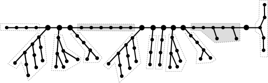
Figure 6.3: An example of a path-like tree. Cut vertices of its fine partition drawn bigger. Shrubs are drawn by a dashed line. Internal shrubs are drawn on gray background.

In order not to clutter this overview with too many technical details, we chose to explain the embedding procedure on a rather simple type of trees: “path-like” trees. With the term path-like trees we mean trees having the property that the deletion of the external shrubs and the contraction of the internal shrubs, with respect to their fine-partition, leads to a path. See Figure 6.3. Our motivation for working with path-like trees in this overview is that if the tree $T$ is more complex we face the complication of parallel branching of the embedding procedure. (This complication is handled by using the stochastic process $\mathsf{Duplicate}$ as outlined in [HKP⁺a, Section LABEL:p0.sssec:whyGexp].) Note that, however, the family of path-like trees is general enough that it contains trees with any given ratio of internal shrubs and end shrubs.

At every step of the embedding procedure, we will avoid the sets $U_{i}$ and $F_{i}$, making an exception for the roots of internal shrubs, which may be mapped even to $F_{2}\setminus U_{2}$. It will be clear from the following, why we need this exception and why we can afford it. Note that at the beginning of our embedding procedure, the sets $U_{i},F_{i}$ are all empty, and thus trivial to avoid.

As outlined in Table 6.2,we shall make use of the setting of $\mathbf{(exp)}$ to embed hubs, of $\mathbf{(\heartsuit 1)}$ to embed the end shrubs, and the specifics of Configuration $\mathbf{(\diamond 7)}$ will be used for embedding the internal shrubs.

Embedding the first hub

We start by embedding the hub containing a fixed root $R$ of $T$ mapping $W_{A}$ to $V_{1}$ and mapping $W_{B}$ to $V_{0}$. The hubs are only of size $O(1)$ by Definition 3.3(c). So, the mere minimum degree conditions (5.34) and (5.35) are sufficient for embedding the hub while avoiding the sets $U_{0}$ and $U_{1}$. In addition, we wish to avoid the set $F_{1}$. While embedding the first hub , we have not embedded any internal shrub yet. Therefore, initially, the set $U_{2}$ is empty, and so is the set $F_{1}$.

Figure 6.4: Embedding an internal shrub in Section 6.1.3. A suitable dense spot $D$ shown dashed.

The rest of the embedding combines three techniques: embedding internal shrubs, embedding hubs, and embedding end shrubs.

Embedding an internal shrub

Assume that we are at a given time of the embedding process when we have just finished embedding some hub and are about to embed the next internal shrub $T^{*}$. A picture corresponding to the description below is given in Figure 6.4. As the predecessor $p$ of the root $r$ of the shrub is mapped to $V_{1}$, (5.41) tells us that the image of $p$ has a substantial degree into $V_{2}$. Since $p$ was mapped outside of $F_{1}$, the image of $p$ has a substantial degree to $V_{2}\setminus U_{2}$. The set $V_{2}\setminus U_{2}$ has the avoiding property (see Definition 4.5), and therefore only very few candidates should not be used for the accomodating $r$, as they are exceptional with respect to the set $U_{3}\cup F_{3}$ (which is of size $O(k)$ by (6.1)). Therefore, we can map $r$ to some non-exceptional vertex in $V_{2}\setminus U_{2}$. In order to embed the children $q_{1},\ldots,q_{\ell}$ of $r$ we shall use the property of the avoiding set, i.e., we use that there is a dense spot $D$ containing the image of $r$ such that

$$|D\cap(U_{3}\cup F_{3})|\leqslant\gamma^{2}k\;.$$ (6.2)

As the image of $r$ has substantial minimal degree in $D\cap\mathbb{A}_{1}$ by Setting 5.4(4) and only a very small portion of it goes outside of $V_{3}$ (by (5.43)) or to $U_{3}\cup F_{3}$ (by (6.2)), we can map $q_{1},\ldots,q_{\ell}$ to $V_{3}\setminus(U_{3}\cup F_{3})$ (recall that $\ell\leqslant\tau k$, and $\tau$ is the smallest constant in our hierarchy).

The minimum degree condition (5.44) together with the fact that the children $q_{1},\ldots,q_{\ell}$ were embedded outside of $F_{3}$ this will ensure that we can map the grandchildren $q^{\prime}_{1},\ldots,q^{\prime}_{\ell^{\prime}}$ of $r$ to $V_{2}$ while avoiding the set $U_{2}\cup F_{2}$.

As we have seen above, it is enough to avoid $U_{2}$ and the set of exceptional vertices in $V_{2}$ (in the sense of the avoiding set) to be able to further extend the embedding of the internal shrub, by finding (possibly different) dense spots $D_{1}^{\prime},\ldots,D_{\ell^{\prime}}^{\prime}$ containing $q_{1}^{\prime},\ldots,q_{\ell}^{\prime}$, respectively, such that $|D_{i}^{\prime}\cap(U_{3}\cup F-3)|\leqslant\gamma^{2}k$. We repeat this process until the embedding of $T^{*}$ is finished.

The idea behind defining the set $F_{2}$ is to prevent getting stuck when we need to map the next seed from $W_{A}$ to the set $V_{1}\setminus(U_{1}\cup F_{1})$, as here again we have no structural information on $V_{2}$ or between $V_{2}$ and $V_{1}$ we can exploit (the avoiding property is useful only to go from $V_{2}$ to $V_{3}$, as it can be combined with the negligible loss of degree outside $V_{3}$).

Before we turn our attention to further parts of the embedding process let us meditate on the reason for allowing the embedding of the root $r$ of $T^{*}$ in $F_{2}$ and why we can afford such an exception. If we had to avoid the set $F_{2}$ for the embedding of the roots of the internal shrubs, we would need to include a shadow of $F_{2}$ in $F_{1}$. On the other hand, the set $F_{2}$ includes a shadow of $F_{1}$, so this would create a loop in the definitions. We can afford this exception for the following reason. For any vertex mapped to $V_{2}\setminus F_{2}$, we can ensure that if it has a child belonging to $W_{A}$, then this child can be mapped to $V_{1}\setminus(U_{1}\cup F_{1})$. This however is not guaranteed for the roots of the internal shrubs. Therefore, it is important that no root of internal shrub has a child belonging to $W_{A}$. This is the reason behind Property (i) of Definition 3.3.

Embedding further hubs

Recall that the first hub has already been embedded. We shall now explain how we make use of the expanding property of $G_{\mathrm{exp}}$ from Preconfiguration $\mathbf{(exp)}$ to embed any further hub $X$. First, note that the first vertex of $X$ we are about to embed can be mapped to a suitable $w\in V_{1}\setminus(U_{1}\cup F_{1})$, as its predecessor $q$ (which was a part of a previous internal shrub) does not belong to $F_{2}$. Hence, let us assume that any vertex $x\in W_{A}$ is mapped to some vertex $w\in V_{1}\setminus(U_{1}\cup F_{1})$. We want to pick a prospective candidate among the neighbours of $w$ to which we shall map any given child of $x$. The only properties required from this candidate is to be unused and to have substantial degree to $V_{1}\setminus(U_{1}\cup F_{1})$. Only a tiny fraction of the neighbours of $w$ lie in $U_{0}$, as the size of $W_{A}\cup W_{B}$ is $O(1)$ by Definition 3.3(c). By (5.34), any vertex in $\mathrm{N}(w)\cap(V_{0}\setminus U_{0})$ is a suitable prospective candidate, except those that send many edges to $U_{1}\cup F_{1}$ (in $G_{\mathrm{exp}}$). However, there are only very few such vertices by Fact 4.13. Thus, (5.34) tells us that we can accomodate $x$.

One could argue that while embedding the hubs and internal shrubs, the sets $U_{i}$, and thus $F_{i}$, do increase dynamically. However, this is not a real problem and can easily be dealt with. Indeed, in every step of our embedding process, we have a substantial number of candidates we can choose from (of the order of magnitude $\delta k$). The size of one hub, respectively of one internal tree, is of a much smaller order. Therefore, it is enough to update the sets $U_{i}$ and $F_{i}$ only at certain times.

Embedding $\mathcal{S}_{B}$-shrubs

Once we have embedded all hubs and all internal shrubs, we start embedding shrubs that are adjacent to $W_{B}$. By Definition 3.3(k) these are end shrubs. As explained in [HKP⁺b, Section LABEL:p1.sssec:roughversusfine], the embedding of the end shrubs is much easier since we do not have to return to $V_{0}$ and $V_{1}$ for embedding cut vertices.

Let us note that at this stage of the embedding process no vertex of $\mathbb{A}_{2}$, and thus of $V_{\mathrm{good}}^{\restriction{2}}$, has been used. The total order of the end shrubs is about $h_{2}\approx\mathfrak{p}_{2}k$. Definition 3.3(l) tells us that the total order of $\mathcal{S}_{B}$ is at most $h_{2}/2$. Display (5.30) tells us that the degree of the vertices in $V_{0}$ to $V_{\mathrm{good}}^{\restriction{2}}$ is at least $h_{2}/2$. As we suspend the embedding of the end shrubs adjacent to vertices in $W_{A}$ until the last stage, there are always enough unused neighbours of vertices from $V_{0}$ lying in $V_{\mathrm{good}}^{\restriction{2}}$. To extend the embedding from a root to the entire end shrub it corresponds to, we use our basic techniques that build on the avoiding property, on the properties of the nowhere-dense graph, or on exploiting regular pairs. The definitions (5.8) and (5.5) indeed provide us with a setting in which it is possible to extend the embedding from $V_{\mathrm{good}}$ as explained in [HKP⁺b, Section LABEL:p1.ssec:motivation]. The order in which we embed the $\mathcal{S}_{B}$-shrubs is important in order to fill the end-clusters of regular pairs of $(\mathcal{M}_{A}\cup\mathcal{M}_{B})^{\restriction{2}}$ at the same pace as long as possible.

Embedding $\mathcal{S}_{A}$-end shrubs

It remains to embed the end shrubs from $\mathcal{S}_{A}$. We shall use the same techniques we used for $\mathcal{S}_{B}$-shrubs.

By (5.31), the minimum degree from $V_{1}$ to $V_{\mathrm{good}}^{\restriction{2}}$ is at least $h_{2}$ and the total order of all end shrubs (including those from $\mathcal{S}_{B}$) is slightly less than $h_{2}$. Therefore, there are always sufficient unused neighbours of vertices from $V_{1}$ in $V_{\mathrm{good}}^{\restriction{2}}$. Finally, (5.32) means that we do not need to care whether we fill of the end-clusters of regular pairs of $(\mathcal{M}_{A}\cup\mathcal{M}_{B})^{\restriction{2}}$ in a balanced way.

6.1.4 Embedding overview for Configuration $\mathbf{(\diamond 8)}$

Suppose we are in Setting 5.1 and 5.4. We are working with sets $V_{0}$, $V_{1}$, $V_{\mathrm{good}}^{\restriction{2}}$, $V_{2},V_{3}$ and $V_{4}$ and with a regularized matching $\mathcal{N}$ coming from the configuration.

The embedding scheme follows Table 6.2, and is illustrated in Figure 6.5.

Figure 6.5: An overview of embedding a fine partition $(W_{A},W_{B},\mathcal{S}_{A},\mathcal{S}_{B})$ of a tree $T\in\mathbf{trees}({k})$ using Configuration $\mathbf{(\diamond 8)}$. The hubs are embedded between $V_{0}$ and $V_{1}$. The roots of the internal shrubs are embedded in $V_{2}$. Some of the subshrubs of the internal shrubs are embedded in $V_{3}\cup V_{4}$ and some in $\mathcal{N}$; principal subshrubs are always embedded in $V_{3}\cup V_{4}$. The end shrubs are embedded using the properties of $V_{\mathrm{good}}^{\restriction{2}}$.

The embedding of the hubs and of the external shrubs is done in the same way as in Configurations $\mathbf{(\diamond 6)}$–$\mathbf{(\diamond 7)}$. We only describe here the way the internal shrubs are embedded. Their roots are embedded in $V_{2}$. From that point we proceed embedding subshrub by subshrub. Some of the subshrubs get embedded between $V_{3}$ and $V_{4}$. This pair of sets has the same expansion property as the pair $V_{2},V_{3}$ in Configuration $\mathbf{(\diamond 7)}$. In particular, it allows to avoid the shadow of the already occupied set so that the follow-up hub can be embedded in a location almost isolated from the previous images, similarly as described in Section 6.1.2. For this reason we make sure that principal subshrubs get embedded here. The degree condition from $V_{2}$ to $V_{3}$ is too weak to ensure that all remaining subshrubs are embedded between $V_{3}$ and $V_{4}$. Therefore we might have to embed some subshrubs in $\mathcal{N}$. Condition (5.51) — where $h_{1}$ is approximately the order of the internal shrubs, as in Remark 6.1 — indicates that it should be possible to accommodate all the subshrubs. For technical reasons, the order in which different types of subshrubs are embedded is very important.

6.1.5 Embedding overview for Configuration $\mathbf{(\diamond 9)}$

The embedding process in Configuration $\mathbf{(\diamond 9)}$ follows the same scheme as in Configurations $\mathbf{(\diamond 6)}$–$\mathbf{(\diamond 8)}$, but the embedding of the internal shrubs follows the regularity method. Assuming the simplest situation $\mathcal{F}=\mathcal{V}_{2}(\mathcal{N})$ and $V_{2}=V_{1}(\mathcal{N})$, we would have $\mathrm{mindeg}_{G_{\mathrm{reg}}}(V_{1},V_{1}(\mathcal{N}))\geqslant h_{1}$ (cf. (5.52)). See Figure 6.6 for an illustration.

Figure 6.6: An overview of embedding a fine partition $(W_{A},W_{B},\mathcal{S}_{A},\mathcal{S}_{B})$ of a tree $T\in\mathbf{trees}({k})$ using Configuration $\mathbf{(\diamond 9)}$. The hubs are embedded between $V_{0}$ and $V_{1}$, the internal shrubs using the regularity method in $\mathcal{N}$ and the end shrubs are embedded using $V_{\mathrm{good}}^{\restriction{2}}$.

Similarly as above, the hubs are embedded between $V_{0}$ and $V_{1}$. The internal shrubs are accommodated using the regularity method in $\mathcal{N}$, and the end shrubs are embedded in $V_{\mathrm{good}}^{\restriction{2}}$ using Preconfiguration $\mathbf{(\heartsuit 1)}$. The embedding lemma for this configuration is given in Lemma 6.26.

6.1.6 Embedding overview for Configuration $\mathbf{(\diamond 10)}$

Configuration $\mathbf{(\diamond 10)}$ is very closely related to the structure obtained by Piguet and Stein [PS12] in their solution of the dense approximate case of Conjecture 1.1.

Theorem 6.2 (Piguet–Stein [PS12]).

For any $q>0$ and $\alpha>0$ there exists a number $n_{0}$ such that for any $n>n_{0}$ and $k>qn$ the following holds. Each $n$-vertex graph $G$ with at least $n/2$ vertices of degree at least $(1+\alpha)k$ contains each tree of order $k+1$.

Let us describe their proof first. Piguet and Stein prove that when $k>qn$ (for some fixed $q>0$ and $k$ sufficiently large) the cluster graph $\mathbf{G}_{\mathrm{reg}}$ of a graph $G\in\mathbf{LKS}({n},{k},{\eta})$ contains the following structure (cf. [PS12, Lemma 8]). There is a set of clusters $\mathbf{L}\subseteq\mathbf{V}$ such that each cluster in $\mathbf{L}$ contains only vertices of captured degrees at least $(1+\frac{\eta}{2})k$. There is a matching $M\subseteq\mathbf{G}_{\mathrm{reg}}$, and an edge $AB$, with $A,B\in\mathbf{L}$. One of the following conditions is satisfied

1. $M$ covers $\mathrm{N}_{\mathbf{G}_{\mathrm{reg}}}(\{A,B\})$, or

2. $M$ covers $\mathrm{N}_{\mathbf{G}_{\mathrm{reg}}}(A)$, and the vertices in $B$ have captured degrees at least $(1+\frac{\eta}{2})\frac{k}{2}$ into $\bigcup(\mathbf{L}\cup V(M))$. Further, each edge in $M$ has at most one endvertex in $\mathrm{N}_{\mathbf{G}_{\mathrm{reg}}}(A)$.

Piguet and Stein use structures (H1) and (H2) to embed any given tree $T\in\mathbf{trees}({k})$ into $G$ using the regularity method; see Sections 3.6 and 3.7 in [PS12], respectively. Actually, a slight relaxation of (H1) and (H2) would be sufficient for the embedding to work, as can be easily seen from their proof: Again, there is a set of clusters $\mathbf{L}\subseteq\mathbf{V}$ such that each cluster in $\mathbf{L}$ contains only vertices of captured degrees at least $(1+\frac{\eta}{2})k$, there is a matching $M\subseteq\mathbf{G}_{\mathrm{reg}}$, and an edge $AB$, $A,B\in\mathbf{L}$. One of the following conditions is satisfied

1. the vertices in $A\cup B$ have captured degrees at least $(1+\frac{\eta}{2})k$ into the vertices of $\bigcup(\mathbf{L}\cup V(M))$, or

2. the vertices in $A$ have captured degrees at least $(1+\frac{\eta}{2})k$ into the vertices of $\bigcup V(M)$, and the vertices in $B$ have captured degrees at least $(1+\frac{\eta}{2})\frac{k}{2}$ into $\bigcup(\mathbf{L}\cup V(M))$. Further, each edge in $M$ has at most one endvertex in $\mathrm{N}_{\mathbf{G}_{\mathrm{reg}}}(A)$.

It can be seen that Configuration $\mathbf{(\diamond 10)}$ is a direct counterpart to (H1’). (The counterpart of (H2’) is contained in Configuration $\mathbf{(\diamond 9)}$ and the similarity is somewhat weaker.)

The embedding lemma for Configuration $\mathbf{(\diamond 10)}$ is stated in Lemma 6.27.

6.2 The role of random splitting

The random splitting as introduced in Setting 5.4 is used in Configurations $\mathbf{(\diamond 6)}$–$\mathbf{(\diamond 9)}$; the set $\mathbb{A}_{0}$ will host the cut-vertices $W_{A}\cup W_{B}$, the set $\mathbb{A}_{1}$ will host the internal shrubs, and the set $\mathbb{A}_{2}$ will (essentially) host the end shrubs of a $(\tau k)$-fine partition of $T_{\mathrm{T}\ref{thm:main}}$.

The need for introducing the random splitting is dictated by Configurations $\mathbf{(\diamond 6)}$–$\mathbf{(\diamond 9)}$. To see this, let us try to follow the embedding plan from, for example, Section 6.1.2 without the random splitting, i.e., dropping the conditions $\subseteq\mathbb{A}_{0}$, $\subseteq\mathbb{A}_{1}$, $\subseteq\mathbb{A}_{2}$ from Definitions 5.12–5.17. Then the sets $V_{2}$ and $V_{3}$ in Figure 6.2, which will host the internal shrubs, may interfere with $V_{0}$ and $V_{1}$ primarily designated for $W_{A}$ and $W_{B}$. In particular, the conditions on degrees between $V_{0}$ and $V_{1}$ given by (5.34)–(5.35) in Definition 5.14, or given by the super-regularity in Definition 5.15 (in which $\beta_{{\mathrm{D}\ref{def:exp8}}}>0$, or $d^{\prime}_{{\mathrm{D}\ref{def:reg}}}\mu_{{\mathrm{D}\ref{def:reg}}}>0$ are tiny) may be insufficient for embedding greedily all the cut-vertices and all the internal shrubs of $T_{\mathrm{T}\ref{thm:main}}$. It should be noted that this problem occurs even in Preconfiguration $\mathbf{(exp)}$, i.e., the expanding property does not add enough strength to the minimum degree conditions. Restricting $V_{0}$ and $V_{1}$ to host only the cut-vertices (only $O(1/\tau)=o(k)$ of them in total, cf. Definition 3.3(c)), resolves the problem.

The above justifies the distinction between the space $\mathbb{A}_{0}$ for embedding the cut-vertices and the space $\mathbb{A}_{1}\cup\mathbb{A}_{2}$ for embedding the shrubs. There are some other approaches which do not need to further split $\mathbb{A}_{1}\cup\mathbb{A}_{2}$ but doing so seems to be the most convenient.

6.3 Stochastic process $\mathsf{Duplicate}(\ell)$

Let us introduce a class of stochastic processes, which we call *Duplicate@$\mathsf{Duplicate}(\ell)$$\mathsf{Duplicate}(\ell)$ ($\ell\in\mathbb{N}$). These are discrete processes $(X_{1},Y_{1}),(X_{2},Y_{2}),\ldots,(X_{q},Y_{q})\in\{0,1\}^{2}$ (where $q\in\mathbb{N}$ is arbitrary) satisfying the following.

• For each $i\in[q]$, we have either

  1. $X_{i}=Y_{i}=0$ (deterministically), or

  2. $X_{i}=Y_{i}=1$ (deterministically), or

  3. exactly one of $X_{i}$ and $Y_{i}$ is one, and in that case $\mathbf{P}[X_{i}=1]=\frac{1}{2}$.

• If the distribution of $(X_{i},Y_{i})$ is according to (c), then the random choice is made independently of the values $(X_{j},Y_{j})$ ($j<i$).

• We have $\sum_{i=1}^{q}(X_{i}+Y_{i})\leqslant\ell$.

We note that this definition is not deep and its purpose is only to adopt the language we shall use later. The following lemma asserts that the first and second components of a process $\mathsf{Duplicate}(\ell)$ are typically balanced.

Lemma 6.3.

Suppose that $(X_{1},Y_{1}),(X_{2},Y_{2}),\ldots,(X_{q},Y_{q})$ is a process in $\mathsf{Duplicate}(\ell)$. Then for any $a>0$ we have

$$\mathbf{P}\left[\sum_{i=1}^{q}X_{q}-\sum_{i=1}^{q}Y_{q}\geqslant a\right]\leqslant\exp\left(-\frac{a^{2}}{2\ell}\right)\;.$$

Proof.

We shall use the following version of the Chernoff bound for sums of independent random variables $Z_{i}$, with distribution $\mathbf{P}[Z_{i}=1]=\mathbf{P}[Z_{i}=-1]=\frac{1}{2}$.

$$\mathbf{P}\left[\sum_{i=1}^{n}Z_{i}\geqslant a\right]\leqslant\exp\left(-\frac{a^{2}}{2n}\right)\;.$$ (6.3)

Let $J\subseteq[q]$ be the set of all indices $i$ with $X_{i}+Y_{i}=1$. By the definition of $\mathsf{Duplicate}(\ell)$, we have $|J|\leqslant\ell$. By (6.3) we have

$$\mathbf{P}\left[\sum_{J}(X_{i}-Y_{i})\geqslant a\right]\leqslant\exp\left(-\frac{a^{2}}{2|J|}\right)\leqslant\exp\left(-\frac{a^{2}}{2\ell}\right)\;.$$

∎

We shall use the stochastic process $\mathsf{Duplicate}$ to guarantee that certain fixed vertex sets do not get overfilled during our tree embedding procedure. $\mathsf{Duplicate}$ is used in Lemmas 6.13 and 6.14 through Lemma 6.12. The way we use $\mathsf{Duplicate}$ was sketched in [HKP⁺a, Section LABEL:p0.sssec:whyGexp].

6.4 Embedding small trees

When embedding the tree $T_{\mathrm{T}\ref{thm:main}}$ in our proof of Theorem 1.2 it will be important to control where different bits of $T_{\mathrm{T}\ref{thm:main}}$ go. This motivates the following notation. Let $X_{1},\ldots,X_{\ell}\subseteq V(T)$ be arbitrary vertex sets of a tree $T$, and let $V_{1},\ldots,V_{\ell}\subseteq V(G)$ be arbitrary vertex sets of a graph $G$. Then an embedding $\phi:V(T)\rightarrow V(G)$ of $T$ in $G$ is an $(X_{1}\hookrightarrow V_{1},\ldots,X_{\ell}\hookrightarrow V_{\ell})$-embedding **embedding@$(X_{1}\hookrightarrow V_{1},\ldots,X_{\ell}\hookrightarrow V_{\ell})$-embedding**embedding@$(X_{1}\hookrightarrow V_{1},\ldots,X_{\ell}\hookrightarrow V_{\ell})$-embedding if $\phi(X_{i})\subseteq V_{i}$ for each $i\in[\ell]$.

We provide several sufficient conditions for embedding a small tree with additional constraints.

The first lemma deals with embeddings using an avoiding set.

Lemma 6.4.

Let $\Lambda,k\in\mathbb{N}$ and let $\varepsilon,\gamma\in(0,\frac{1}{2})$ with $\gamma^{2}>\varepsilon$. Suppose $\mathbb{E}$ is a $(\Lambda,\varepsilon,\gamma,k)$-avoiding set with respect to a set $\mathcal{D}$ of $(\gamma k,\gamma)$-dense spots in a graph $H$. Suppose that $(T_{1},r_{1}),\ldots,(T_{\ell},r_{\ell})$ are rooted trees with $|\bigcup_{i}T_{i}|\leqslant\gamma k/2$. Let $U\subseteq V(H)$ with $|U|\leqslant\Lambda k$, and let $U^{*}\subseteq\mathbb{E}$ with $|U^{*}|\geqslant\varepsilon k+\ell$. Then there are mutually disjoint $(r_{i}\hookrightarrow U^{*},V(T_{i})\setminus\{r_{i}\}\hookrightarrow V(H)\setminus U)$-embeddings of the trees $(T_{i},r_{i})$ in $H$.

Proof.

Since $\mathbb{E}$ is $(\Lambda,\varepsilon,\gamma,k)$-avoiding, there exists a set $Y\subseteq\mathbb{E}$ with $|Y|\leqslant\varepsilon k$, such that each vertex $v$ in $\mathbb{E}\setminus Y$ has degree at least $\gamma k$ into some $(\gamma k,\gamma)$-dense spot $D\in\mathcal{D}$ with $|U\cap V(D)|\leqslant\gamma^{2}k$. In particular, $U^{*}\setminus Y$ is large enough so that we can embed all vertices $r_{i}$ there. We successively extend this embedding to an embedding of $\bigcup_{i}T_{i}$, at each step finding a suitable image in $V(D)\setminus U$ for one neighbour of an already embedded vertex $v\in\bigcup_{i}V(T_{i})$. This is possible since the image of $v$ has degree at least $\gamma k-|U\cap V(D)|>\gamma k/2\geqslant\sum_{i}v(T_{i})$ into $V(D)\setminus U$. ∎

The next lemma deals with embedding a tree into a nowhere-dense graph, a prime example of which is the graph $G_{\mathrm{exp}}$.

Lemma 6.5.

Let $k\in\mathbb{N}$, let $Q\geqslant 1$ and let $\gamma,\zeta\in(0,1)$ be such that $128Q\gamma\leqslant\zeta^{2}$. Let $H$ be a $(\gamma k,\gamma)$-nowhere-dense graph. Let $(T_{1},r_{1}),\ldots,(T_{\ell},r_{\ell})$ be rooted trees of total order less than $\zeta k/4$. Let $V_{1},V_{2},U,U^{*}\subseteq V(H)$ be four sets with $U^{*}\subseteq V_{1}$, $|U|<Qk$, $|U^{*}|>\frac{32Q^{2}\gamma}{\zeta}k+\ell$, and $\mathrm{mindeg}_{H}(V_{j},V_{3-j})\geqslant\zeta k$ for $j=1,2$. Then there are mutually disjoint $(r_{i}\hookrightarrow U^{*},V_{\mathrm{even}}(T_{i})\hookrightarrow V_{1}\setminus U,V_{\mathrm{odd}}(T_{i})\hookrightarrow V_{2}\setminus U)$-embeddings of the trees $(T_{i},r_{i})$ in $H$.

Proof.

Set $B:=\mathrm{shadow}_{H}(U,\zeta k/2)$. By Fact 4.13, we have $|B|\leqslant\frac{32Q^{2}\gamma}{\zeta}k\leqslant\zeta k/4$. In particular, $U^{*}\setminus B$ is large enough to accommodate the images $\phi(r_{i})$ of all vertices $r_{i}$.

Successively, extend $\phi$, in each step mapping a neighbour $u$ of some already embedded vertex $v\in\bigcup_{i}V(T_{i})$ to a yet unused neighbour of $\phi(v)$ in $V_{j}\setminus(B\cup U)$, where $j$ is either 1 or 2, depending on the parity of $\mathrm{dist}_{T}(r,v)$. This is possible as $\phi(v)$, lying outside $B$, has at least $\zeta k/2$ neighbours in $V_{i}\setminus U$. Thus $\phi(v)$ has at least $\zeta k/4$ neighbours in $V_{i}\setminus(U\cup B)$, which is more than $\sum_{i}v(T_{i})$. ∎

The next three lemmas (Lemma 6.7–6.9) deal with embedding trees in a regular or a super-regular pair. Before stating them, we give an auxiliary lemma that will be used in the proof of Lemma 6.8.

Lemma 6.6.

Let $\{x_{i}\}_{i=1}^{s}$, $\{y_{i}\}_{i=1}^{s}$ be two families of reals in $[0,K]$, with $\sum_{i}x_{i}>0$. Write $X:=\sum_{i}x_{i}$, $Y:=\sum_{i}y_{i}$, and $\gamma:=Y/X$. Then for each $X^{\prime}\in[0,X]$ there is a set $I\subseteq[s]$ such that

1. $\sum_{i\in I}x_{i}\leqslant X^{\prime}\leqslant\sum_{i\in I}x_{i}+K$, and

2. $\sum_{i\in I}y_{i}-K\leqslant\gamma X^{\prime}\leqslant\sum_{i\in I}y_{i}+2K$.

Proof.

Inductively construct sets $J_{\ell}\subseteq[s]$ as follows for $\ell=1,\ldots,s$. We start by setting $J_{1}=\emptyset$. In step $\ell$, if $\gamma\sum_{j\in J_{\ell}}x_{j}\geqslant\sum_{j\in J_{\ell}}y_{j}$, then choose $j_{\ell}\in[s]\setminus J_{\ell}$ such that $\gamma x_{j_{\ell}}\leqslant y_{j_{\ell}}$. Otherwise, take $j_{\ell}\in[s]\setminus J_{\ell}$ with $\gamma x_{j_{\ell}}>y_{j_{\ell}}$. The existence of such an index $j_{\ell}$ follows by averaging. Set $J_{\ell+1}:=J_{\ell}\cup\{j_{\ell}\}$. Our procedure ensures that for each $\ell$ we have

$$\sum_{j\in J_{\ell}}y_{j}-K\leqslant\gamma\sum_{j\in J_{\ell}}x_{j}\leqslant\sum_{j\in J_{\ell}}y_{j}+K.$$ (6.4)

Now for a given $X^{\prime}$, let $p$ be the largest integer such that $\sum_{j\in J_{p}}x_{j}\leqslant X^{\prime}$. Setting $I:=J_{p}$, we clearly have (a), while the first inequality in (b) holds because of (6.4) (first inequality) for $\ell=p$. For the second inequality in (b), it is enough to focus on the case $p\neq s$, as otherwise $X=X^{\prime}$ and consequently $\gamma X^{\prime}=\sum_{i\in I}y_{j}$. But then, by the definition of $p$ and by (6.4) (second inequality) for $\ell=p+1$,

$$\gamma X^{\prime}\leqslant\gamma\sum_{i\in J_{p+1}}x_{i}\leqslant\sum_{i\in J_{p+1}}y_{i}+K\leqslant\sum_{i\in I}y_{i}+2K,$$

as desired. ∎

Lemma 6.7.

Let $\varepsilon>0$ and $\beta>2\varepsilon$. Let $(C,D)$ be an $\varepsilon$-regular pair in a graph $H$, with $|C|=|D|=:\ell$, and with density $\mathrm{d}(C,D)\geqslant 3\beta$. Suppose that there are sets $X\subseteq C$, $Y\subseteq D$, and $X^{*}\subseteq X$ satisfying $\min\{|X|,|Y|\}\geqslant 4\frac{\varepsilon}{\beta}\ell$ and $|X^{*}|>\frac{\beta}{2}\ell$. Let $(T,r)$ be a rooted tree of order $v(T)\leqslant\varepsilon\ell$. Then there exists an $(r\hookrightarrow X^{*},V_{\mathrm{even}}(T)\hookrightarrow X,V_{\mathrm{odd}}(T)\hookrightarrow Y)$-embedding of $T$ in $H$.

Proof.

We shall construct an embedding $\phi:V(T)\rightarrow X\cup Y$ satisfying the requirements of the lemma. Fact 2.1 implies that $(X,Y)$ is $\beta/2$-regular of density greater than $2\beta$. By Fact 2.2, there are sets $X^{\prime}\subseteq X$ and $Y^{\prime}\subseteq Y$ with $|X^{\prime}|>(1-\beta/2)|X|$ and $|Y^{\prime}|>(1-\beta/2)|Y|$ such that $\mathrm{mindeg}(X^{\prime},Y)\geqslant\frac{3}{2}\beta|Y|$, $\mathrm{mindeg}(Y^{\prime},X)\geqslant\frac{3}{2}\beta|X|$. Then

$$\begin{split}\mathrm{mindeg}(H[X^{\prime},Y^{\prime}])\geqslant\beta\min\{|X|,|Y|\}\geqslant 2\varepsilon\ell>v(T).\end{split}$$ (6.5)

Choose any vertex in $X^{*}\cap X^{\prime}$ (which is non-empty by the above calculations) for $\phi(r)$. By (6.5) we can greedily extend $\phi$ to an embedding $\phi:V(T)\rightarrow X^{\prime}\cup Y^{\prime}$. ∎

Lemma 6.8.

Let $\beta,\varepsilon>0$ and $\ell\in\mathbb{N}$ be such that $\varepsilon\leqslant\beta^{2}/8$. Let $(C,D)$ be an $\varepsilon$-regular pair with $|C|=|D|=\ell$ of density $\mathrm{d}(C,D)\geqslant 3\beta$ in a graph $H$. Let $(T_{1},r_{1}),(T_{2},r_{2}),\ldots,(T_{s},r_{s})$ be rooted trees with $v(T_{i})\leqslant\varepsilon\ell$ for all $i\in[s]$. Let $U\subseteq V(H)$ fulfill $|C\cap U|=|D\cap U|$, and let $X^{*}\subseteq(C\cup D)\setminus U$ be such that

$$|X^{*}|\geqslant\sum_{i=1}^{s}v(T_{i})+50\beta\ell\;.$$ (6.6)

Then there are mutually disjoint $(r_{i}\hookrightarrow X^{*},V(T_{i})\hookrightarrow(C\cup D)\setminus U)$-embeddings of the trees $(T_{i},r_{i})$ in $H$.

Proof.

Let us write $M:=|X^{*}\cap C|$ and $m:=|X^{*}\cap D|$. Without loss of generality, we assume that $M\geqslant m$. For each $i\in[s]$, let us write $a_{i}$ and $b_{i}$ for the number of vertices of $T_{i}$ at even and odd distance from $r_{i}$, respectively. Furthermore, we write $A:=\sum_{i}a_{i}$, $B:=\sum_{i}b_{i}$, and $\gamma:=B/A$. In a first step, we shall partition the set $[s]$ into three sets $I_{1},I_{2}$, and $I^{\prime\prime}$, according to three cases:

• $m\leqslant 4\beta\ell$,

• $m>4\beta\ell$, and $2(m-4\beta\ell)\geqslant A+B$,

• $m>4\beta\ell$, and $2(m-4\beta\ell)<A+B$.

Once this has been done, we will show how to embed the rooted trees $T_{i}$, using this partition.

In Case (C1), we set $I_{1}=I_{2}:=\emptyset$, and $I^{\prime\prime}:=[s]$. For Cases (C2), and (C3), we first partition $[s]$ into two sets $I$ and $I^{\prime\prime}$ and will make use of an auxiliary set $I^{\prime}$ in order to obtain $I_{1}$ and $I_{2}$ as follows. In Case (C2), set $I:=[s]$, $I^{\prime\prime}:=\emptyset$, and $I^{\prime}:=I$. In Case (C3), we apply Lemma 6.6 with input $(x_{i})_{i\in[s]}:=(a_{i})_{i\in[s]}$, $(y_{i})_{i\in[s]}:=(b_{i})_{i\in[s]}$, $X^{\prime}:=\frac{2A}{A+B}(m-4\beta\ell)$, and the bound $K:=\frac{\beta}{4}\ell$. The bound $X^{\prime}\leqslant X=A$ required in Lemma 6.6 follows from the second property of Case (C3). The lemma yields a set $I\subseteq[s]$ such that

$$\sum_{I}a_{i} \leqslant\frac{2A}{A+B}(m-4\beta\ell)\;,$$ (6.7)

$$\frac{2A}{A+B}(m-4\beta\ell) \leqslant\sum_{I}a_{i}+\frac{\beta}{4}\ell\;,$$ (6.8)

$$\sum_{I}b_{i}-\frac{\beta}{4}\ell \leqslant\frac{2B}{A+B}(m-4\beta\ell)\;\mbox{, and}$$ (6.9)

$$\frac{2B}{A+B}(m-4\beta\ell) \leqslant\sum_{I}b_{i}+\frac{\beta}{2}\ell\;.$$ (6.10)

Bound (6.8) can be used to bound $\sum_{I^{\prime\prime}}a_{i}$ for the complementary set $I^{\prime\prime}:=[s]\setminus I$ as follows.

$$\sum_{I^{\prime\prime}}a_{i} \leqslant A-\left(\frac{2A}{A+B}(m-4\beta\ell)-\frac{\beta}{4}\ell\right)=A\left(1-\frac{2(m-4\beta\ell)}{A+B}\right)+\frac{\beta}{4}\ell$$

$$\leqslant(M+m-50\beta\ell)\left(1-\frac{2(m-4\beta\ell)}{M+m-50\beta\ell}\right)+\frac{\beta}{4}\ell\leqslant M-m-40\beta\ell\;,$$ (6.11)

where we employed the bound $A\leqslant A+B\leqslant M+m-50\beta\ell$ from (6.6). Likewise, we have from (6.10) that

$$\sum_{I^{\prime\prime}}b_{i}\leqslant M-m-40\beta\ell\;.$$ (6.12)

The main feature of Lemma 6.6 is that the ratio $\sum_{I}b_{i}:\sum_{I}a_{i}$ is almost exactly $\gamma$. In order to even out a small imperfection we may have, let us introduce a dummy pair $(a_{0},b_{0})$, with $0<a_{0},b_{0}\leqslant\beta\ell/2$ such that for $I^{\prime}:=I\cup\{0\}$, we have

$$\frac{\sum_{I^{\prime}}b_{i}}{\sum_{I^{\prime}}a_{i}}=\gamma\;.$$

The existence of such a pair $(a_{0},b_{0})$ follows from the properties of Lemma 6.6.

In Cases (C2), and (C3), we apply Lemma 6.6 to further partition the set $I$. More specifically, the input of Lemma 6.6 consists of $X^{\prime}:=\frac{A}{A+B}(m-4\beta\ell)$, $(x_{i})_{i\in I^{\prime}}:=(a_{i})_{i\in I^{\prime}}$, $(y_{i})_{i\in I^{\prime}}:=(b_{i})_{i\in I^{\prime}}$, and $K:=\frac{\beta}{2}\ell$. Lemma 6.6 gives an index set $J_{1}\subseteq I^{\prime}$. Set $I_{1}:=J_{1}\setminus\{0\}\subseteq I$. We have that

$$\sum_{I_{1}}a_{i} \leqslant\frac{A}{A+B}(m-4\beta\ell)\;,$$ (6.13)

$$\frac{A}{A+B}(m-4\beta\ell) \leqslant\sum_{I_{1}}a_{i}+\beta\ell\;,$$ (6.14)

$$\sum_{I_{1}}b_{i}-\frac{\beta}{2}\ell \leqslant\frac{B}{A+B}(m-4\beta\ell)\;\mbox{, and}$$ (6.15)

$$\frac{B}{A+B}(m-4\beta\ell) \leqslant\sum_{I_{1}}b_{i}+\frac{3}{2}\beta\ell\;.$$ (6.16)

Set $I_{2}:=I\setminus I_{1}$. From (6.7) and (6.14) we have

$$\sum_{I_{2}}a_{i}\leqslant\frac{2A}{A+B}(m-4\beta\ell)-\left(\frac{A}{A+B}(m-4\beta\ell)-\beta\ell\right)=\frac{A}{A+B}(m-4\beta\ell)+\beta\ell\;.$$ (6.17)

Similarly, (6.9) and (6.16) give

$$\sum_{I_{2}}b_{i}\leqslant\frac{B}{A+B}(m-4\beta\ell)+2\beta\ell\;.$$ (6.18)

We shall now see how the partition $[s]=I_{1}\cup I_{2}\cup I^{\prime\prime}$ gives us instructions to embed the trees $T_{1},\ldots,T_{s}$ one by one. The trees $T_{i}$, $i\in I_{1}$ are embedded in the bipartite graph $(W,(D\cap X^{*})\setminus U)$, where $W$ is an arbitrary subset of $C\cap X^{*}$ of size $m$, with the root $r_{i}$ embedded in $W$. The trees $T_{i}$, $i\in I_{2}$ are embedded in the bipartite graph $(D\cap X^{*},W)$, with the root $r_{i}$ embedded in $D\cap X^{*}$. Finally, the trees $T_{i}$, $i\in I^{\prime\prime}$ are embedded in $((C\cap X^{*})\setminus W,D\setminus(X^{*}\cup U))$, with the root embedded in $(C\cap X^{*})\setminus W$. We can embed the trees $(T_{i})_{i\in I_{1}\cup I_{2}}$ as described above, by repetitively using Lemma 6.7, as we have enough space for the embeddings: summing up (6.13) and (6.18) we have

$$\sum_{I_{1}}a_{i}+\sum_{I_{2}}b_{i}\leqslant m-4\beta\ell+2\beta\ell=|W|-2\beta\ell\;,$$

and similarly from (6.15) and (6.17) we have

$$\sum_{I_{1}}b_{i}+\sum_{I_{2}}a_{i}\leqslant m-4\beta\ell+\frac{3}{2}\beta\ell\leqslant|D\cap X^{*}|-2\beta\ell\;.$$

Likewise, the trees $(T_{i})_{i\in I^{\prime\prime}}$ can be embedded in $((C\cap X^{*})\setminus W,D\setminus(X^{*}\cup U))$ with the help of Lemma 6.7, as (6.11) says that $\sum_{I^{\prime\prime}}a_{i}\leqslant|(C\cap X^{*})\setminus W|-40\beta\ell$, and as (6.12) says that $\sum_{I^{\prime\prime}}b_{i}\leqslant|(C\cap X^{*})\setminus W|-40\beta\ell\leqslant|D\setminus(X^{*}\cup U)|-40\beta\ell$. ∎

Lemma 6.9.

Let $d>10\varepsilon>0$. Suppose that $(A,B)$ forms an $(\varepsilon,d)$-super-regular pair with $|A|,|B|\geqslant\ell$. Let $U_{A}\subseteq A$, $U_{B}\subseteq B$ be such that $|U_{A}|\leqslant|A|/2$ and $|U_{B}|\leqslant d|B|/4$. Let $(T,r)$ be a rooted tree of order at most $d\ell/4$, and let $v\in A\setminus U_{A}$ be arbitrary. Then there exists an $(r\hookrightarrow v,V_{\mathrm{even}}(T,r)\hookrightarrow A\setminus U_{A},V_{\mathrm{odd}}(T,r)\hookrightarrow B\setminus U_{B})$-embedding of $T$.

Sketch of the proof.

The lemma is a variant of Lemma 6.7 with only two qualitative differences. Firstly, the assumptions of the lemma are stronger in that we now have super-regularity rather than regularity. Secondly, the assertion of the lemma is stronger in that we can map the root of the tree on a specific vertex $r\hookrightarrow v$, rather than into a specified set $r_{\mathrm{L}\ref{lem:embed:regular}}\hookrightarrow X^{*}_{\mathrm{L}\ref{lem:embed:regular}}$. The proof scheme of Lemma 6.7 indeed gives this stronger assertion under the current assumptions. To see this, note that in the proof of Lemma 6.7, it was enough to map $r$ to an arbitrary vertex which had enough degree to the destination set ($B\setminus U_{B}$, in the present lemma) of its children. In the current setting, any $v\in A\setminus U_{A}$ can serve as such a vertex as $\deg(v,B\setminus U_{B})\geqslant\deg(v,B)-|U_{B}|\geqslant d|B|-d|B|/4=\frac{3}{4}d|B|$, where the last inequality uses the super-regularity of $(A,B)$. ∎

Suppose that we have to embed a rooted tree $(T,r)$, and its root was already mapped on a vertex $\phi(r)$. Suppose that $r$ has degree $\ell_{X}+\ell_{Y}$ in a regular pair $(X,Y)$, where $\ell_{X}:=\deg(\phi(r),X),\ell_{Y}:=\deg(\phi(r),Y)$, with $\ell_{X}\geqslant\ell_{Y}$, say. The hope is that we can embed $T$ in $(X,Y)$ as long as $v(T)$ is a bit smaller than $\ell_{X}+\ell_{Y}$. For this, the greedy strategy does not work (see Figure 6.7) and we need to be somewhat more careful.

Figure 6.7: An example of a rooted tree $(T,r)$, depicted on the left. The forest $T-r$ has three components (I), (II), (III) of total order 12. Say the vertex $r$ is embedded so that for the regular pair $(X,Y)$ we have $\deg(\phi(r),X)=8$, $\deg(\phi(r),Y)=4$ (neighbourhoods of $\phi(r)$ hatched). While the greedy strategy does not work (middle), splitting the process into a balanced and an unbalanced stage (right) does — here the components (I) and (II) are embedded in the balanced stage and the component (III) in the unbalanced stage.

We split the embedding process into two stages. In the first stage we choose a subset of the components of $T-r$ of total order approximately $2\min\big{(}\ell_{X},\ell_{Y}\big{)}=2\ell_{Y}$. When embedding these, we choose orientations of each component in such a way that the image is approximately balanced with respect to $X$ and $Y$. In the second stage we embed the remaining components so that their roots are embedded in $X$. We refer to the first stage as balanced way of embeddingunbalanced way of embeddingembedding in a balanced way, and to the second stage as embedding in an unbalanced way.

The next lemma says that each regular pair can be filled-up in a balanced way by trees.

Lemma 6.10.

Let $G$ be a graph, $v\in V(G)$ be a vertex, $\mathcal{M}$ be an $(\varepsilon,d,\nu k)$-regularized matching in $G$, and $\{f_{CD}\}_{(C,D)\in\mathcal{M}}$ be a family of integers between $-\tau k$ and $\tau k$. Suppose $(T,r)$ is a rooted tree,

$$v(T)\leqslant\left(1-\frac{4(\varepsilon+\frac{\tau}{\nu})}{d-2\varepsilon}\right)|V(\mathcal{M})|\;,$$

with the property that each component of $T-r$ has order at most $\tau k$. If $V(\mathcal{M})\subseteq\mathrm{N}_{G}(v)$ then there exists an $(r\hookrightarrow v,V(T-r)\hookrightarrow V(\mathcal{M}))$-embedding $\phi$ of $T$ such that for each $(C,D)\in\mathcal{M}$ we have $|C\cap\phi(T)|+f_{CD}=|D\cap\phi(T)|\pm\tau k$.

The proof of Lemma 6.10 is standard, and is given for example in [HP16, Lemma 5.12].

Lemma 6.10 suggests the following definitions. The discrepancydiscrepancy of a set $X$ with respect to a pair of sets $(C,D)$ is the number $|C\cap X|-|D\cap X|$. $X$ is $s$-balancedbalanced set with respect to a regularized matching $\mathcal{M}$ if the discrepancy of $X$ with respect to each $(C,D)\in\mathcal{M}$ is at most $s$ in absolute value.

Lemma 6.11.

Let $G$ be a graph, $v\in V(G)$ be a vertex, $\mathcal{M}$ be an $(\varepsilon,d,\nu k)$-regularized matching in $G$ with an $\mathcal{M}$-cover $\mathcal{F}$, and $U\subseteq V(G)$. Suppose $(T,r)$ is a rooted tree with

$$v(T)+|U|\leqslant\deg_{G}\left(v,V(\mathcal{M})\setminus\bigcup\mathcal{F}\right)-\frac{4(\varepsilon+\frac{\tau}{\nu})}{d-2\varepsilon}|V(\mathcal{M})|\;,$$

such that each component of $T-r$ has order at most $\tau k$. Then there exists an $(r\hookrightarrow v,V(T-r)\hookrightarrow V(\mathcal{M})\setminus U)$-embedding $\phi$ of $T$.

The proof of Lemma 6.11 is again standard and we again omit it.

The following lemma uses a probabilistic technique to embed a shrub while reserving a set of vertices in the host graph for later use. We wish the reserved set to use about as much space inside certain given sets $P_{i}$ as the image of our shrub does. (In later applications the sets $P_{i}$ correspond to neighbourhoods of vertices which are still ‘active’.)

Lemma 6.12 will find an immediate application in all the remaining lemmas of this subsection. However it is really necessary only for Lemmas 6.13–6.14, which deal with embedding shrubs in the presence of one of the Configurations $\mathbf{(\diamond 6)}$–$\mathbf{(\diamond 8)}$. For Lemmas 6.15 and 6.16, which are for Configurations $\mathbf{(\diamond 3)}$ and $\mathbf{(\diamond 4)}$, a simpler auxiliary lemma (without reservations) would suffice.

Lemma 6.12.

Let $H$ be a graph, let $X^{*},X_{1},X_{2},P_{1},P_{2},\ldots,P_{L}\subseteq V(H)$, and let $(T_{1},r_{1})$, …, $(T_{\ell},r_{\ell})$ be rooted trees, such that $L\leqslant k$, $|P_{j}|\leqslant k$ for each $j\in[L]$, and $|X^{*}|\geqslant 2\ell$. Suppose that $\mathrm{mindeg}(X_{1}\cup X^{*},X_{2})\geqslant 2\sum v(T_{i})$ and $\mathrm{mindeg}(X_{2},X_{1})\geqslant 2\sum v(T_{i})$.

Then there exist pairwise disjoint $\left(r_{i}\hookrightarrow X^{*},V_{\mathrm{even}}(T_{i},r_{i})\setminus\{r_{i}\}\hookrightarrow X_{1},V_{\mathrm{odd}}(T_{i},r_{i})\hookrightarrow X_{2}\right)$-embeddings $\phi_{i}$ of $T_{i}$ in $G$ and a set $C\subseteq(X_{1}\cup X_{2})\setminus\bigcup\phi_{i}(T_{i})$ of size $\sum v(T_{i})$ such that for each $j\in[L]$ we have

$$|P_{j}\cap\bigcup\phi_{i}(T_{i})|\leqslant|P_{j}\cap C|+k^{3/4}.$$ (6.19)

Proof.

Let $m:=\sum v(T_{i})$.

We construct pairwise disjoint random $\left(r_{i}\hookrightarrow X^{*},V_{\mathrm{even}}(T_{i},r_{i})\setminus\{r_{i}\}\hookrightarrow X_{1},V_{\mathrm{odd}}(T_{i},r_{i})\hookrightarrow X_{2}\right)$-embeddings $\phi_{i}$ and a set $C\subseteq V(H)\setminus\bigcup\phi_{i}(T_{i})$ which satisfies (6.19) with positive probability. Then the statement follows.

Enumerate the vertices of $\bigcup T_{i}$ as $\bigcup V(T_{i})=\{v_{1},\ldots,v_{m}\}$ such that $v_{i}=r_{i}$ for $i=1,\ldots,\ell$, and such that for each $j>\ell$ we have that the parent of $v_{j}$ lies is the set $\{v_{1},\ldots,v_{j-1}\}$. Pick pairwise disjoint sets $A_{1},\ldots,A_{\ell}\subseteq X^{*}$ of size two. Choose uniformly and independently at random an element $x_{j}\in A_{j}$. Denote the other element of $A_{j}$ as $y_{j}$.

Now, successively for $i=\ell+1,\ldots,m$, we shall define vertices $x_{i}$ and $y_{i}$. Let $r$ denote the root of the tree in which $v_{i}$ lies, and let $v_{s}=\mathrm{Par}(v_{i})$ be the parent of $v_{i}$. We shall choose $x_{i},y_{j}\in X_{j_{i}}$ where $j_{i}=\mathrm{dist}(r,v_{i})\mod 2+1$. In step $i$, proceed as follows. Since $x_{s}\in X_{j_{s}}$ (or since $x_{s}\in X^{*}$), we have

$$\deg(x_{s},X_{j_{i}}\setminus\bigcup_{h<i}\{x_{h},y_{h}\})\geqslant 2.$$

Hence, we may take an arbitrary subset $A_{i}\subseteq(\mathrm{N}(x_{s})\cap X_{{j_{i}}})\setminus\bigcup_{h<i}\{x_{h},y_{h}\}$ of size exactly two. As above, randomly label its elements as $x_{i}$ and $y_{i}$ independently of all other choices.

The choices of the maps $(v_{j}\mapsto x_{j})_{j=1}^{m}$ determine $\phi_{1},\ldots,\phi_{\ell}$. Then $C:=\{y_{1},\ldots,y_{m}\}$ has size exactly $m$ and avoids $\bigcup\phi_{i}(T_{i})$.

For each $j\in[L]$ we set up a stochastic process $\mathfrak{S}^{(j)}=\left((X_{i}^{(j)},Y_{i}^{(j)})\right)_{i=1}^{m}$, defined by $X^{(j)}_{i}=\mathbf{1}_{\{x_{i}\in P_{j}\}}$ and $Y^{(j)}_{i}=\mathbf{1}_{\{y_{i}\in P_{j}\}}$. Note that $\mathfrak{S}^{(j)}\in\mathsf{Duplicate}(|P_{j}|)\subseteq\mathsf{Duplicate}(k)$. Thus, for a fixed $j\in[L]$, by Lemma 6.3, the probability that $|P_{j}\cap(\bigcup\phi_{i}(T_{i}))|>|P_{j}\cap C|+k^{3/4}$ is at most $\exp(-\sqrt{k}/2)$. Using the union bound over all $j\in[L]$ we get that Property 6.21 holds with probability at least

$$1-L\cdot\exp\left(-\frac{\sqrt{k}}{2}\right)>0\;.$$

This finishes the proof. ∎

We now get to the first application of Lemma 6.12.

Lemma 6.13.

Assume we are in Setting 5.1. Suppose that we are given sets $V_{2},V_{3}\subseteq V(G)$ are such that we have

$$\mathrm{mindeg}_{H}(V_{2},V_{3})\geqslant\delta k\quad\mbox{and}\quad\mathrm{mindeg}_{H}(V_{3},V_{2})\geqslant\delta k,$$ (6.20)

where $\delta>300/k$, and $H$ is a $(\gamma k,\gamma)$-nowhere dense subgraph of $G$. Suppose that $U,U^{*},P_{1},P_{2},\ldots,P_{L}\subseteq V(G)$, and $L\leqslant k$, are such that $|U|\leqslant\frac{\delta}{24\sqrt{\gamma}}k$, $U^{*}\subseteq V_{2}$, $|U^{*}|\geqslant\frac{\delta}{4}k$, and $|P_{j}|\leqslant k$ for each $j\in[L]$. Let $(T,r)$ be a rooted tree of order at most $\delta k/8$.

Then there exists a $\left(r\hookrightarrow U^{*},V_{\mathrm{even}}(T,r)\setminus\{r\}\hookrightarrow V_{2}\setminus U,V_{\mathrm{odd}}(T,r)\hookrightarrow V_{3}\setminus U\right)$-embedding $\phi$ of $T$ in $G$ and a set $C\subseteq(V_{2}\cup V_{3})\setminus(U\cup\phi(T))$ of size $v(T)$ such that for each $j\in[L]$ we have

$$|P_{j}\cap\phi(T)|\leqslant|P_{j}\cap C|+k^{3/4}.$$ (6.21)

Proof.

Set $B:=\mathrm{shadow}_{G_{\mathrm{exp}}}(U,\delta k/4)$. By Fact 4.13, we have that $|B|\leqslant 64\frac{\gamma}{\delta}(\frac{\delta}{24\sqrt{\gamma}})^{2}k\leqslant\frac{\delta}{4}k-2$. In particular, $X^{*}:=U^{*}\setminus B$ has size at least $2$. Set $X_{1}:=V_{2}\setminus(U\cup B)$ and set $X_{2}:=V_{3}\setminus(U\cup B)$. Using (6.20), we find that

$$\mathrm{mindeg}_{G_{\mathrm{exp}}}(X_{1},X_{2})\geqslant\delta k-\mathrm{maxdeg}_{G_{\mathrm{exp}}}(X_{1},U)-|B|\geqslant\delta k-\frac{\delta}{4}k-\frac{\delta}{4}k\geqslant 2v(T)\;,$$

and similarly, $\mathrm{mindeg}_{G_{\mathrm{exp}}}(X_{2},X_{1})\geqslant 2v(T)$. We may thus apply Lemma 6.12 to obtain the desired embedding $\phi$ and the set $C$. ∎

Lemma 6.14.

Assume Setting 5.1 and Setting 5.4. Suppose that we are given sets $Y_{1},Y_{2}\subseteq\mathbb{A}_{1}\setminus\bar{V}$ with $Y_{1}\subseteq\mathbb{E}$, and

1. $\mathrm{maxdeg}_{G_{\mathcal{D}}}(Y_{1},\mathbb{A}_{1}\setminus Y_{2})\leqslant\frac{\eta\gamma}{400}$, and

2. $\mathrm{mindeg}_{G_{\mathcal{D}}}(Y_{2},Y_{1})\geqslant\delta k$.

Suppose that $U,U^{*},P_{1},P_{2},\ldots,P_{L}\subseteq V(G)$ are sets such that $|U|\leqslant\frac{\Lambda\delta}{2\Omega^{*}}k$, $U^{*}\subseteq Y_{1}$, with $|U^{*}|\geqslant\frac{\delta}{4}k$, $|P_{j}|\leqslant k$ for each $j\in[L]$, and $L\leqslant k$. Suppose $(T_{1},r_{1}),\ldots,(T_{\ell},r_{\ell})$ are rooted trees of total order at most $\delta k/1000$. Suppose further that $\delta<\eta\gamma/100$, $\varepsilon^{\prime}<\delta/1000$, and $k>1000/\delta$.

Then there exist pairwise disjoint $\left(r_{i}\hookrightarrow U^{*},V_{\mathrm{even}}(T_{i},r_{i})\hookrightarrow Y_{1}\setminus U,V_{\mathrm{odd}}(T_{i},r_{i})\hookrightarrow Y_{2}\setminus U\right)$-embeddings $\phi_{i}$ of $T_{i}$ in $G$ and a set $C\subseteq V(G-\bigcup\phi_{i}(T_{i}))$ of size $\sum v(T_{i})$ such that for each $j\in[L]$ we have that

$$|P_{j}\cap\bigcup\phi_{i}(T_{i})|\leqslant|P_{j}\cap C|+k^{3/4}.$$ (6.22)

Proof.

Set $U^{\prime}:=\mathrm{shadow}_{G_{\mathcal{D}}}(U,\delta k/2)\cup U$. By Fact 4.12, we have $|U^{\prime}|\leqslant\Lambda k$. As $Y_{1}$ is a $(\Lambda,\varepsilon^{\prime},\gamma,k)$-avoiding set, by Definition 4.5 there exists a set $B\subseteq Y_{1}$, $|B|\leqslant\varepsilon^{\prime}k$ such that for all $v\in Y_{1}\setminus B$ there exists a dense spot $D_{v}\in\mathcal{D}$ with $v\in V(D_{v})$ and $|V(D_{v})\cap U^{\prime}|\leqslant\gamma^{2}k$. As $Y_{1}$ is disjoint from $\bar{V}$, by Definition 5.3(4) and by (5.13), we have that $\deg_{D_{v}}(v,V(D_{v})^{\restriction{1}})\geqslant\frac{\eta\gamma}{200}k$. By (i), we have that $\deg_{G_{\mathcal{D}}}(v,V(D_{v})^{\restriction{1}}\setminus Y_{2})<\frac{\eta\gamma}{400}k$, and hence,

$$\deg_{G_{\mathcal{D}}}\big{(}v,(V(D_{v})^{\restriction{1}}\cap Y_{2})\setminus U^{\prime}\big{)}\geqslant\frac{\eta\gamma k}{400}-\gamma^{2}k\geqslant\frac{\eta\gamma k}{800}\;.$$

Thus,

$$\mathrm{mindeg}_{G_{\mathcal{D}}}(Y_{1}\setminus B,Y_{2}\setminus(U^{\prime}\cup B))\geqslant\frac{\eta\gamma k}{800}-\varepsilon^{\prime}k\geqslant 2\sum v(T_{i})\;.$$ (6.23)

Further, by the definition of $U^{\prime}$ and by (ii), we have

$$\mathrm{mindeg}_{G_{\mathcal{D}}}(Y_{2}\setminus U^{\prime},Y_{1}\setminus(U\cup B))\geqslant\frac{\delta k}{2}-\varepsilon^{\prime}k\geqslant 2\sum v(T_{i})\;.$$ (6.24)

Set $X^{*}:=U^{*}\setminus B$, and note that $|X^{*}|\geqslant\delta k/4-\varepsilon^{\prime}k\geqslant 2\ell$. Set $X_{1}:=Y_{1}\setminus(U\cup B)$ and $X_{2}:=Y_{2}\setminus(U^{\prime}\cup B)$. Inequalities (6.23) and (6.24) guarantee that we may apply Lemma 6.12 to obtain the desired embeddings $\phi_{i}$. ∎

Lemma 6.15.

Assume Setting 5.1. Suppose that the sets $L^{\prime},L^{\prime\prime},\mathbb{H}^{\prime},\mathbb{H}^{\prime\prime},V_{1},V_{2}$ witness Configuration $\mathbf{(\diamond 3)}(0,0,\gamma/4,\delta)$. Suppose that $U,U^{*}\subseteq V(G)$ are sets such that $|U|\leqslant k$, $U^{*}\subseteq V_{1}$, $|U^{*}|\geqslant\frac{\delta}{4}k$. Suppose $(T,r)$ is a rooted tree of order at most $\delta k/1000$. Suppose further that $\delta\leqslant\gamma/100$, $\varepsilon^{\prime}<\delta/1000$, and $4\Omega^{*}/\delta\leqslant\Lambda$.

Then there is an $\left(r\hookrightarrow U^{*},V_{\mathrm{even}}(T,r)\setminus\{r\}\hookrightarrow V_{1}\setminus U,V_{\mathrm{odd}}(T,r)\hookrightarrow V_{2}\setminus U\right)$-embedding of $T$ in $G$.

Proof.

The proof of this lemma is very similar to the one of Lemma 6.14 (in fact, even easier). Set $U^{\prime}:=\mathrm{shadow}_{G_{\mathcal{D}}}(U,\delta k/2)\cup U$ and note that $|U^{\prime}|\leqslant\Lambda k$ by Fact 4.12. As $V_{1}$ is $(\Lambda,\varepsilon^{\prime},\gamma,k)$-avoiding, by Definition 4.5 there is a set $B\subseteq V_{1}$, $|B|\leqslant\varepsilon^{\prime}k$ such that for all $v\in V_{1}\setminus B$ there exists a dense spot $D_{v}\in\mathcal{D}$ with $\deg_{D_{v}}(v,V(D_{v})\setminus U^{\prime})\geqslant\gamma k/2$. By (5.20), we know that $\deg_{G_{\mathcal{D}}}(v,V(D_{v})\setminus V_{2})\leqslant\gamma k/4$, and hence, $\deg_{G_{\mathcal{D}}}\big{(}v,(V(D_{v})\cap V_{2})\setminus U^{\prime}\big{)}\geqslant\gamma k/{4}$. Thus,

$$\mathrm{mindeg}_{G_{\mathcal{D}}}(V_{1}\setminus B,V_{2}\setminus U^{\prime})\geqslant\frac{\gamma k}{4}\geqslant 2v(T)\;.$$ (6.25)

Further, by the definition of $U^{\prime}$ and by (5.21), we have

$$\mathrm{mindeg}_{G_{\mathcal{D}}}(V_{2}\setminus U^{\prime},V_{1}\setminus U)\geqslant\frac{\delta k}{2}\geqslant 2v(T)\;.$$ (6.26)

Set $X^{*}:=U^{*}\setminus B$, and note that $|X^{*}|\geqslant\delta k/4-\varepsilon^{\prime}k\geqslant 2$. Set $X_{1}:=V_{1}\setminus(U\cup B)$ and $X_{2}:=V_{2}\setminus(U^{\prime}\cup B)$. Inequalities (6.25) and (6.26) guarantee that we may apply Lemma 6.12 (with empty sets $P_{i}$) to obtain the desired embedding $\phi$. ∎

Lemma 6.16.

Assume Setting 5.1. Suppose that the sets $L^{\prime},L^{\prime\prime},\mathbb{H}^{\prime},\mathbb{H}^{\prime\prime},V_{1},\mathbb{E}^{\prime},V_{2}$ witness Configuration $\mathbf{(\diamond 4)}(0,0,\gamma/4,\delta)$. Suppose that $U\subseteq V(G)$, $U^{*}\subseteq V_{1}$ are sets such that $|U|\leqslant k$ and $|U^{*}|\geqslant\frac{\delta}{4}k$. Suppose $(T,r)$ is a rooted tree of order at most $\delta k/20$ with a fruit $r^{\prime}$. Suppose further that $4\varepsilon^{\prime}\leqslant\delta\leqslant\gamma/100$, and $\Lambda\geqslant 300(\frac{\Omega^{*}}{\delta})^{3}$.

Then there exists an $\left(r\hookrightarrow U^{*},r^{\prime}\hookrightarrow V_{1}\setminus U,V(T)\setminus\{r,r^{\prime}\}\hookrightarrow(\mathbb{E}^{\prime}\cup V_{2})\setminus U\right)$-embedding of $T$ in $G$.

Proof.

Set

$$U^{\prime}:=\tilde{U}\cup\mathrm{shadow}_{G_{\nabla}-\mathbb{H}}(U,\delta k/4)\cup\mathrm{shadow}^{(2)}_{G_{\nabla}-\mathbb{H}}(\tilde{U},\delta k/4)$$

and let

$$U^{\prime\prime}:=\tilde{U}\cup\mathrm{shadow}_{G_{\mathcal{D}}}(U^{\prime},\delta k/2).$$

We use Fact 4.12 to see that $|U^{\prime}|\leqslant\frac{\delta}{4\Omega^{*}}\Lambda k$ and $|U^{\prime\prime}|\leqslant\Lambda k$. We then use Definition 4.5 and (5.25) to find a set $B\subseteq\mathbb{E}^{\prime}$ of size at most $\varepsilon^{\prime}k$ such that

$$\mathrm{mindeg}_{G_{\mathcal{D}}}(\mathbb{E}^{\prime}\setminus B,V_{2}\setminus U^{\prime\prime})\geqslant 2v(T)\;.$$ (6.27)

Using (6.27), and employing (5.22) and  (5.24), we see that we may apply Lemma 6.12 with $X^{*}_{\mathrm{L}\ref{lem:randomshrubembedding}}:=U^{*}$, $X_{1,{\mathrm{L}\ref{lem:randomshrubembedding}}}:=\mathbb{E}^{\prime}\setminus(B\cup U^{\prime})$ and $X_{2,{\mathrm{L}\ref{lem:randomshrubembedding}}}:=V_{2}\setminus U^{\prime\prime}$ (and with empty sets $P_{i}$) in order to embed the tree $T-T(r,\uparrow r^{\prime})$ rooted at $r$. Then embed $T(r,\uparrow r^{\prime})$, by applying Lemma 6.12 a second time, using (5.22) and (5.23). ∎

6.5 Main embedding lemmas

For this section, we need to introduce the notion of a ghost. The idea behind this notion is that once we used a set $U$ for the embedding of our tree, the remainder of the graph cannot be used as before. Namely, if $U$ covers part of a cluster of some matching edge, then we will not be able to fill up the partner cluster using usual regularity embedding techniques. The ghost of $U$ will block the unusable part of the partner cluster, and we will know that we cannot expect to fill it up.

Given a regularized matching $\mathcal{N}$, we call an involution $\mathfrak{d}:V(\mathcal{N})\rightarrow V(\mathcal{N})$ with the property that $\mathfrak{d}(S)=T$ for each $(S,T)\in\mathcal{N}$ a matching involutionmatching involution.

Assume Setting 5.1 and fix a matching involution $\mathfrak{b}$ for $\mathcal{M}_{A}\cup\mathcal{M}_{B}$. For any set $U\subseteq V(G)$ we then define ghost*GHOST@$\mathrm{ghost}(U)$

$$\mathrm{ghost}(U):=U\cup\mathfrak{b}\big{(}U\cap V(\mathcal{M}_{A}\cup\mathcal{M}_{B})\big{)}\;.$$

Clearly, we have that $|\mathrm{ghost}(U)|\leqslant 2|U|$, and $|\mathrm{ghost}(U)\cap S|=|\mathrm{ghost}(U)\cap T|$ for each $(S,T)\in\mathcal{M}_{A}\cup\mathcal{M}_{B}$.

The notion of a ghost extends to other regularized matchings. If $\mathcal{N}$ is a regularized matching and $\mathfrak{d}$ is a matching involution for $\mathcal{N}$ then we write $\mathrm{ghost}_{\mathfrak{d}}(U):=U\cup\mathfrak{d}\big{(}U\cap V(\mathcal{N})\big{)}$.

6.5.1 Embedding in Configuration $\mathbf{(\diamond 1)}$

This subsection contains an easy observation that each tree of order $k$ is contained in $G$ if the graph $G$ contains Configuration $\mathbf{(\diamond 1)}$.

Lemma 6.17.

Let $G$ be a graph, and let $A,B\subseteq V(G)$ be such that $\mathrm{mindeg}(G[A,B])\geqslant k/2$, and $\mathrm{mindeg}(A)\geqslant k$. Then each tree of order $k$ is contained in $G$.

Proof.

Let $T\in\mathbf{trees}({k})$ have colour classes $X$ and $Y$, with $|X|\geqslant k/2\geqslant|Y|$. By Fact 3.2, for the set $W$ of those leaves of $T$ that lie in $X$, we have $|X\setminus W|\leqslant k/2$. We embed $T-W$ greedily in $G$, mapping $Y$ to $A$ and $X\setminus W$ to $B$. We then embed $W$ using the fact that $\mathrm{mindeg}(A)\geqslant k$. ∎

6.5.2 Embedding in Configurations $\mathbf{(\diamond 2)}$–$\mathbf{(\diamond 5)}$

In this section we show how to embed $T_{\mathrm{T}\ref{thm:main}}$ in the presence of configurations $\mathbf{(\diamond 2)}$–$\mathbf{(\diamond 5)}$. As outlined in Section 6.1.1 our main embedding lemma, Lemma 6.20, builds on Lemma 6.19 which handles Stage 1 of the embedding, and Lemma 6.18 which handles Stage 2.

Lemma 6.18.

Assume we are in Setting 5.1. Suppose $L^{\prime\prime},L^{\prime},\mathbb{H}^{\prime}$ witness Preconfiguration $\mathbf{(\clubsuit)}(\frac{10^{5}\Omega^{*}}{\eta})$. Let $(T,r)$ be a rooted tree of order at most $\gamma^{2}\nu k/6$. Let $U\subseteq V(G)$ with $|U|+v(T)\leqslant k$, and let $v\in\mathbb{H}^{\prime}\setminus U$. Then there exists an $(r\hookrightarrow v,V(T)\hookrightarrow V(G)\setminus U)$-embedding of $(T,r)$.

Proof.

We proceed by induction on the order of $T$. The base case $v(T)\leqslant 2$ obviously holds. Let us assume Lemma 6.18 is true for all trees $T^{\prime}$ with $v(T^{\prime})<v(T)$.

Let $U_{1}:=\mathrm{shadow}_{G_{\nabla}}(U-\mathbb{H},\eta k/200)$, and $U_{2}:=\bigcup\{C\in\mathbf{V}\>:\>|C\cap U|\geqslant\frac{1}{2}|C|\}$. We have $|U_{1}|\leqslant\frac{200\Omega^{*}}{\eta}k$ by Fact 4.12, and $|U_{2}|\leqslant 2|U|$. Set

$$L_{\mathbb{E}} :=L^{\prime}\cap\mathrm{shadow}_{G_{\nabla}}\left(\mathbb{E},\frac{\eta k}{50}\right),$$

$$L_{\mathbb{H}} :=L^{\prime}\cap\mathrm{shadow}_{G_{\nabla}}\left(\mathbb{H},|U\cap\mathbb{H}|+\frac{\eta k}{50}\right),\text{ and }$$

$$L_{\mathbf{V}} :=L^{\prime}\cap\mathrm{shadow}_{G_{\mathrm{reg}}}\left(V({G_{\mathrm{reg}}}),(1+\frac{\eta}{50})k-|U\cap\mathbb{H}|\right)\;.$$

Observe that $L_{\mathbf{V}}\subseteq\bigcup\mathbf{V}$ and that since $L^{\prime}\subseteq\mathbb{L}_{{\frac{9}{10}\eta},{k}}({G_{\nabla}})\setminus\mathbb{H}$, we have

$$L^{\prime}\subseteq V(G_{\mathrm{exp}})\cup\mathbb{E}\cup L_{\mathbb{H}}\cup L_{\mathbb{E}}\cup L_{\mathbf{V}}\;.$$

As by (5.18), we have $\deg_{G}(v,L^{\prime})\geqslant\frac{10^{5}\Omega^{*}k}{\eta}>5(|U\cup U_{1}\cup U_{2}|+v(T)+\eta k)$, one of the following five cases must occur.

Case I: $\deg_{G}(v,V(G_{\mathrm{exp}})\setminus U)>v(T)+\eta k$. Lemma 6.5 gives an embedding of the forest $T-r$ (whose components are rooted at neighbours of $r$). The input sets/parameters of Lemma 6.5 are $Q_{\mathrm{L}\ref{lem:embed:greyFOREST}}:=1$, $\zeta_{\mathrm{L}\ref{lem:embed:greyFOREST}}:=12\sqrt{\gamma}$, $U^{*}_{\mathrm{L}\ref{lem:embed:greyFOREST}}:=(\mathrm{N}_{G}(v)\cap V(G_{\mathrm{exp}}))\setminus U$, $U_{\mathrm{L}\ref{lem:embed:greyFOREST}}:=U$, and $V_{1}=V_{2}:=V(G_{\mathrm{exp}})$.

Case II: $\deg_{G}(v,\mathbb{E}\setminus U)>v(T)+\eta k$. Lemma 6.4 gives an embedding of the forest $T-r$ (whose components are rooted at neighbours of $r$). The input sets/parameters of Lemma 6.4 are $U^{*}_{\mathrm{L}\ref{lem:embed:avoidingFOREST}}:=(\mathrm{N}_{G}(v)\cap\mathbb{E})\setminus U$, $U_{\mathrm{L}\ref{lem:embed:avoidingFOREST}}:=U$ and $\varepsilon_{\mathrm{L}\ref{lem:embed:avoidingFOREST}}:=\varepsilon^{\prime}\leqslant\eta$. Here, and below, we implicitly assume parameters of the same name to be the same, i.e. $\gamma_{\mathrm{L}\ref{lem:embed:avoidingFOREST}}:=\gamma$.

Case III: $\deg_{G}(v,L_{\mathbb{E}}\setminus(U\cup U_{1}))>v(T)+\eta k$. We only outline the strategy. Embed the children of $r$ in $L_{\mathbb{E}}\setminus(U\cup U_{1})$ using a map $\phi:\mathrm{Ch}_{T}(r)\rightarrow L_{\mathbb{E}}\setminus(U\cup U_{1})$. By definition of $L_{\mathbb{E}}$, and $U_{1}$, we have $\deg_{G_{\nabla}}(\phi(w),\mathbb{E}\setminus U)>\frac{\eta k}{100}$ for each $w\in\mathrm{Ch}_{T}(r)$. Now, for every $w\in\mathrm{Ch}_{T}(r)$ we can proceed as in Case II to extend this embedding to the rooted tree $\big{(}T(r,\uparrow w),w\big{)}$. That is, Case III is “Case II with an extra step in the beginning”.

Case IV: $\deg_{G}(v,L_{\mathbb{H}}\setminus U)>v(T)+\eta k$. We embed the children $\mathrm{Ch}_{T}(r)$ of $r$ in distinct vertices of $L_{\mathbb{H}}\setminus U$. This is possible by the assumption of Case IV.

Now, (5.17) implies that $\mathrm{mindeg}_{G_{\nabla}}(L_{\mathbb{H}},\mathbb{H}^{\prime})\geqslant|U\cap\mathbb{H}|+\frac{\eta k}{100}$. Consequently, $\mathrm{mindeg}_{G_{\nabla}}(L_{\mathbb{H}},\mathbb{H}^{\prime}\setminus U)\geqslant\frac{\eta k}{100}$. Therefore, for each $w\in\mathrm{Ch}_{T}(r)$ embedded in $L_{\mathbb{H}}\setminus U$ we can find an embedding of $\mathrm{Ch}_{T}(w)$ in $\mathbb{H}^{\prime}\setminus U$ such that the images of grandchildren of $r$ are disjoint. We fix such an embedding. We can now apply induction. More specifically, for each grandchild $u$ of $r$ we embed the rooted tree $\big{(}T(r,\uparrow u),u\big{)}$ using Lemma 6.18 (employing induction) using the updated set $U$, to which the images of the newly embedded vertices were added.

Case V: $\deg_{G}(v,L_{\mathbf{V}}\setminus(U\cup U_{1}\cup U_{2}))\geqslant v(T)$. Let $u_{1},\ldots,u_{\ell}$ be the children of $r$. Let us consider arbitrary distinct neighbours $x_{1},\ldots,x_{\ell}\in L_{\mathbf{V}}\setminus(U\cup U_{1}\cup U_{2})$ of $v$. Let $T_{i}:=T(r,\uparrow u_{i})$. We sequentially embed the rooted trees $(T_{i},u_{i})$, $i=1,\ldots,\ell$, writing $\phi$ for the embedding. In step $i$, consider the set $W_{i}:=\left(U\cup\bigcup_{j<i}\phi(T_{j})\right)\setminus\mathbb{H}$. Let $D_{i}\in\mathbf{V}$ be the cluster containing $x_{i}$. By the definitions of $L_{\mathbf{V}}$ and of $U_{1}$,

$$\deg_{G_{\mathrm{reg}}}(x_{i},V(G_{\mathrm{reg}})\setminus W_{i})\geqslant\frac{\eta k}{50}-\frac{\eta k}{200}\geqslant\frac{\eta k}{100}\;.$$

Fact 4.8 yields a cluster $C_{i}\in\mathbf{V}$ for which

$$\deg_{G_{\mathrm{reg}}}(x_{i},C_{i}\setminus W_{i})\geqslant\frac{\eta}{100}\cdot\frac{\gamma\mathfrak{c}}{2(\Omega^{*})^{2}}>\frac{\gamma^{2}\mathfrak{c}}{2}+v(T)>\frac{12\varepsilon^{\prime}\mathfrak{c}}{\gamma^{2}}+v(T)\;.$$

In particular there is at least one edge from $E(G_{\mathrm{reg}})$ between $C_{i}$ and $D_{i}$, and therefore, $(C_{i},D_{i})$ forms an $\varepsilon^{\prime}$-regular pair of density at least $\gamma^{2}$ in $G_{\mathrm{reg}}$. Map $u_{i}$ to $x_{i}$ and let $F_{1},\ldots,F_{m}$ be the components of the forest $T_{i}-u_{i}$. We now sequentially embed the trees $F_{j}$ in the pair $(D_{i},C_{i})$ using Lemma 6.7, with $X_{\mathrm{L}\ref{lem:embed:regular}}:=C_{i}\setminus(W_{i}\cup\bigcup_{q<j}\phi(F_{q}))$, $X^{*}_{\mathrm{L}\ref{lem:embed:regular}}:=\mathrm{N}_{G_{\mathrm{reg}}}(x_{i},X_{\mathrm{L}\ref{lem:embed:regular}})$, $Y_{\mathrm{L}\ref{lem:embed:regular}}:=D_{i}\setminus(W_{i}\cup\{x_{i}\}\cup\bigcup_{q<j}\phi(F_{q}))$, $\varepsilon_{\mathrm{L}\ref{lem:embed:regular}}:=\varepsilon^{\prime}$, and $\beta_{\mathrm{L}\ref{lem:embed:regular}}:=\gamma^{2}/3$. ∎

We are now ready for the lemma that will handle Stage 1 in configurations $\mathbf{(\diamond 2)}$–$\mathbf{(\diamond 5)}$.

Lemma 6.19.

Assume we are in Setting 5.1, with $L^{\prime\prime},L^{\prime},\mathbb{H}^{\prime}$ witnessing Preconfiguration $\mathbf{(\clubsuit)}(\Omega^{\dagger})$ in $G$. Let $U\subseteq V(G)\setminus\mathbb{H}$ and let $(T,r)$ be a rooted tree with $v(T)\leqslant k/2$ and $|U|+v(T)\leqslant k$. Suppose that each component of $T-r$ has order at most $\tau k$. Let $x\in(L^{\prime\prime}\cap\mathbb{YB})\setminus\bigcup_{i=0}^{2}\mathrm{shadow}_{G_{\nabla}}^{(i)}(\mathrm{ghost}(U),\eta k/1000)$.

Then there is a subtree $T^{\prime}$ of $T$ with $r\in V(T^{\prime})$ which has an $(r\hookrightarrow x,V(T^{\prime})\setminus\{r\}\hookrightarrow V(G)\setminus\mathbb{H})$-embedding $\phi$. Further, the components of $T-T^{\prime}$ can be partitioned into two (possibly empty) families $\mathcal{C}_{1}$ and $\mathcal{C}_{2}$, such that the following two assertions hold.

1. If $\mathcal{C}_{1}\neq\emptyset$, then $\mathrm{mindeg}_{G_{\nabla}}(\phi(\mathrm{Par}(V(\bigcup\mathcal{C}_{1}))),\mathbb{H}^{\prime})>k+\frac{\eta k}{100}-v(T^{\prime})$,

2. $\mathrm{Par}(V(\bigcup\mathcal{C}_{2}))\subseteq\{r\}$, and $\deg_{G_{\nabla}}(x,\mathbb{H}^{\prime})>\frac{k}{2}+\frac{\eta k}{100}-v(T^{\prime}\cup\bigcup\mathcal{C}_{1})$.

Proof.

Let $\mathcal{C}$ be the family of all components of $T-r$. We start by defining $\mathcal{C}_{2}$. Then we have to distribute $T-\bigcup\mathcal{C}_{2}$ between $T^{\prime}$ and $\mathcal{C}_{1}$. First, we find a set $\mathcal{C}_{M}\subseteq\mathcal{C}\setminus\mathcal{C}_{2}$ which fits into the matching $\mathcal{M}_{A}\cup\mathcal{M}_{B}$ (and thus will form a part of $T^{\prime}$). Then, we consider the remaining components of $\mathcal{C}\setminus\mathcal{C}_{2}$: some of these will be embedded entirely, of others we only embed the root, and leave the rest for $\mathcal{C}_{1}$. Everything embedded will become a part of $T^{\prime}$.

Throughout the proof we write $\mathrm{shadow}$ for $\mathrm{shadow}_{G_{\nabla}}$.

Set $\overline{V}_{\mathrm{good}}:=V_{\mathrm{good}}\setminus\mathrm{shadow}(\mathrm{ghost}(U),\frac{\eta k}{1000})$, and choose $\tilde{\mathcal{C}}\subseteq\mathcal{C}$ such that

$$\deg_{G_{\nabla}}(x,\overline{V}_{\mathrm{good}})-\frac{\eta k}{30}\ <\ \sum_{S\in\tilde{\mathcal{C}}}v(S)\ \leqslant\ \max\left\{0,\deg_{G_{\nabla}}\left(x,\overline{V}_{\mathrm{good}}\right)-\frac{\eta k}{40}\right\}.$$ (6.28)

Set $\mathcal{C}_{2}:=\mathcal{C}\setminus\tilde{\mathcal{C}}$. Note that this choice clearly satisfies the first part of (b). Let us now verify the second part of (b). For this, we calculate

$$\deg_{G_{\nabla}}(x,\mathbb{H}^{\prime}) \geqslant\deg_{G_{\nabla}}(x,V_{+}\setminus L_{\#})-\deg_{G_{\nabla}}\left(x,\mathrm{shadow}\left(\mathrm{ghost}(U),\frac{\eta k}{1000}\right)\right)$$

$$~{}~{}~{}~{}-\deg_{G_{\nabla}}\left(x,V_{+}\setminus\left(L_{\#}\cup\mathrm{shadow}\left(\mathrm{ghost}(U),\frac{\eta k}{1000}\right)\cup\mathbb{H}\right)\right)$$

$$~{}~{}~{}~{}-\deg_{G_{\nabla}}(x,\mathbb{H}\setminus\mathbb{H}^{\prime})$$

(by (5.10), $$x\not\in\mathrm{shadow}^{(2)}(\mathrm{ghost}(U),\frac{\eta k}{1000}) \geqslant\left(\frac{k}{2}+\frac{\eta k}{20}\right)-\frac{\eta k}{1000}-\left(\sum_{S\in\tilde{\mathcal{C}}}v(S)+\frac{\eta k}{30}\right)-\frac{\eta k}{100}$$, (6.28), (5.17))

$$>\ \frac{k}{2}-\sum_{S\in\tilde{\mathcal{C}}}v(S)+\frac{\eta k}{20}$$

$$\geqslant\frac{k}{2}-v\left(T^{\prime}\cup\bigcup\mathcal{C}_{1}\right)+\frac{\eta k}{100},$$

as needed for (b).

Now, set

$$\mathcal{M}:=\big{\{}(X_{1},X_{2})\in\mathcal{M}_{A}\cup\mathcal{M}_{B}\>:\>\deg_{G_{\mathcal{D}}}(x,(X_{1}\cup X_{2})\setminus\mathbb{E})>0\big{\}}\;.$$ (6.29)

Claim 6.19.1.

We have $|V(\mathcal{M})|\leqslant\frac{4(\Omega^{*})^{2}}{\gamma^{2}}k$.

Proof of Claim 6.19.1.

Indeed, let $(X_{1},X_{2})\in\mathcal{M}$, i.e. $(X_{1},X_{2})\in\mathcal{M}_{A}\cup\mathcal{M}_{B}$ with $\deg_{G_{\mathcal{D}}}(x,(X_{1}\cup X_{2})\setminus\mathbb{E})>0$. Then, using Property 4 of Setting 5.1, we see that there exists a cluster $C_{(X_{1},X_{2})}\in\mathbf{V}$ such that $\deg_{G_{\mathcal{D}}}(x,C_{(X_{1},X_{2})})>0$, and either $X_{1}\subseteq C_{(X_{1},X_{2})}$ or $X_{2}\subseteq C_{(X_{1},X_{2})}$. In particular, there exists a dense spot $(A_{(X_{1},X_{2})},B_{(X_{1},X_{2})};F_{(X_{1},X_{2})})\in\mathcal{D}$ such that $x\in A_{(X_{1},X_{2})}$, and $X_{1}\subseteq B_{(X_{1},X_{2})}$ or $X_{2}\subseteq B_{(X_{1},X_{2})}$. By Fact 4.4, there are at most $\frac{\Omega^{*}}{\gamma}$ such dense spots, let $Z$ denote the union of all vertices contained in these spots. Fact 4.3 implies that $|Z|\leqslant\frac{2(\Omega^{*})^{2}}{\gamma^{2}}k$. Thus $|V(\mathcal{M})|\leqslant 2|V(\mathcal{M})\cap Z|\leqslant 2|Z|\leqslant\frac{4(\Omega^{*})^{2}}{\gamma^{2}}k$. ∎

First we shall embed as many components from $\tilde{\mathcal{C}}$ in $\mathcal{M}$ as possible. To this end, consider an inclusion-maximal subset $\mathcal{C}_{M}$ of $\tilde{\mathcal{C}}$ with

$$\sum_{S\in\mathcal{C}_{M}}v(S)\leqslant\deg_{G_{\nabla}}(x,V(\mathcal{M}))-\frac{\eta k}{1000}\;.$$ (6.30)

We aim to utilize the degree of $x$ to $V(\mathcal{M})$ to embed $\mathcal{C}_{M}$ in $V(\mathcal{M})$, using the regularity method.

Remark 6.19.2.

This remark (which may as well be skipped at a first reading) is aimed at those readers who are wondering about a seeming inconsistency of the defining formulas (6.29) for $\mathcal{M}$, and (6.30) for $\mathcal{C}_{M}$. That is, (6.29) involves the degree in $G_{\mathcal{D}}$ and excludes the set $\mathbb{E}$, while (6.30) involves the degree in $G_{\nabla}$. The setting in (6.29) was chosen so that it allows us to control the size of $\mathcal{M}$ in Claim 6.19.1, crucially relying on Property 4 of Setting 5.1. Such a control is necessary to make the regularity method work. Indeed, in each regular pair there may be a small number of atypical vertices, and we must avoid these vertices when embedding the components by the regularity method. Thus without the control on $|\mathcal{M}|$ it might happen that the degree of $x$ is unusable because $x$ sees very small numbers of atypical vertices in an enormous number of sets corresponding to $\mathcal{M}$-vertices. On the other hand, the edges $x$ sends to $\mathbb{E}$ can be utilized by other techniques in later stages. Once we have defined $\mathcal{M}$ we want to use the full degree to $V(\mathcal{M})$ to ensure we can embed the shrubs as balanced as possible into the $\mathcal{M}$-edges. This is necessary as otherwise part of the degree of $x$ might be unusable for the embedding, e.g. because it might go to $\mathcal{M}$-vertices whose partners are already full.

For each $(C,D)\in\mathcal{M}$ we choose a family $\mathcal{C}_{CD}\subseteq\mathcal{C}_{M}$ maximal such that

$$\sum_{S\in\mathcal{C}_{CD}}v(S)\leqslant\deg_{G_{\nabla}}\left(x,(C\cup D)\setminus\mathrm{ghost}(U)\right)-\left(\frac{\gamma}{\Omega^{*}}\right)^{3}|C|\;,$$ (6.31)

and further, we require $\mathcal{C}_{CD}$ to be disjoint from families $\mathcal{C}_{C^{\prime}D^{\prime}}$ defined in previous steps. We claim that $\{\mathcal{C}_{CD}\}_{(C,D)\in\mathcal{M}}$ forms a partition of $\mathcal{C}_{M}$, i.e., all the elements of $\mathcal{C}_{M}$ are used. Indeed, otherwise, by the maximality of $\mathcal{C}_{CD}$ and since the components of $T-r$ have size at most $\tau k$, we obtain

$$\begin{split}\sum_{S\in\mathcal{C}_{CD}}v(S)&\geqslant\deg_{G_{\nabla}}(x,(C\cup D)\setminus\mathrm{ghost}(U))-\left(\frac{\gamma}{\Omega^{*}}\right)^{3}|C|-\tau k\\ &\overset{\mbox{\tiny{\eqref{eq:KONST}}}}{\geqslant}\deg_{G_{\nabla}}(x,(C\cup D)\setminus\mathrm{ghost}(U))-2\left(\frac{\gamma}{\Omega^{*}}\right)^{3}|C|\;,\end{split}$$ (6.32)

for each $(C,D)\in\mathcal{M}$. Then we have

$$\sum_{S\in\mathcal{C}_{M}}v(S) >\sum_{(C,D)\in\mathcal{M}}\sum_{S\in\mathcal{C}_{CD}}v(S)$$

(by (6.32)) $$\geqslant\sum_{(C,D)\in\mathcal{M}}\left(\deg_{G_{\nabla}}(x,(C\cup D)\setminus\mathrm{ghost}(U))-2\left(\frac{\gamma}{\Omega^{*}}\right)^{3}|C|\right)$$

(by Claim 6.19.1 and Fact 4.11) $$\geqslant\deg_{G_{\nabla}}\left(x,V(\mathcal{M})\setminus\mathrm{ghost}(U)\right)-2\left(\frac{\gamma}{\Omega^{*}}\right)^{3}\cdot\frac{2(\Omega^{*})^{2}}{\gamma^{2}}k$$

(as $$x\not\in\mathrm{shadow}(\mathrm{ghost}(U)) \geqslant\deg_{G_{\nabla}}(x,V(\mathcal{M}))-\frac{\eta k}{1000}$$)

(by (6.30)) $$\geqslant\sum_{S\in\mathcal{C}_{M}}v(S)\;,$$

a contradiction.

We use Lemma 6.8 to embed the components of $\mathcal{C}_{CD}$ in $(C\cup D)\setminus\mathrm{ghost}(U)$ with the following setting: $C_{\mathrm{L}\ref{lem:fillingCD}}:=C$, $D_{\mathrm{L}\ref{lem:fillingCD}}:=D$, $U_{\mathrm{L}\ref{lem:fillingCD}}:=\mathrm{ghost}(U)$, $X^{*}_{\mathrm{L}\ref{lem:fillingCD}}:=(\mathrm{N}_{G_{\nabla}}(x)\cap(C\cup D))\setminus U_{\mathrm{L}\ref{lem:fillingCD}}$, and $(T_{i},r_{i})$ are the rooted trees from $\mathcal{C}_{CD}$ with the roots being the neighbours of $r$. The constants in Lemma 6.8 are $\varepsilon_{\mathrm{L}\ref{lem:fillingCD}}:=\varepsilon^{\prime}/8$, $\beta_{\mathrm{L}\ref{lem:fillingCD}}:=\sqrt{\varepsilon^{\prime}}$, and $\ell_{\mathrm{L}\ref{lem:fillingCD}}:=|C|\geqslant\nu\pi k$. The rooted trees in $\mathcal{C}_{CD}$ are smaller than $\varepsilon_{\mathrm{L}\ref{lem:fillingCD}}\ell_{\mathrm{L}\ref{lem:fillingCD}}$ by (5.1). Condition (6.6) is satisfied by (6.31), and since $(\gamma/{\Omega^{*}})^{3}\geqslant 50\sqrt{\varepsilon^{\prime}}$.

It remains to deal with the components of $\tilde{\mathcal{C}}\setminus\mathcal{C}_{M}$. In the sequel we shall assume that $\tilde{\mathcal{C}}\setminus\mathcal{C}_{M}\neq\emptyset$ (otherwise skip this step and go directly to the definition of $T^{\prime}$ and $\mathcal{C}_{1}$, with $p=0$). Thus, by our choice of $\mathcal{C}_{M}$, we have

$$\sum_{S\in\mathcal{C}_{M}}v(S)\geqslant\deg_{G_{\nabla}}(x,V(\mathcal{M}))-\frac{\eta k}{900}\;.$$ (6.33)

Let $T_{1},T_{2},\ldots,T_{p}$ be the trees of $\tilde{\mathcal{C}}\setminus\mathcal{C}_{M}$ rooted at the vertices $r_{i}\in\mathrm{Ch}(r)\cap V(T_{i})$ neighbouring $r$. We shall sequentially extend our embedding of $\mathcal{C}_{M}$ to subtrees $T^{\prime}_{i}\subseteq T_{i}$. Let $U_{i}\subseteq V(G)$ be the union of the images of $\bigcup\mathcal{C}_{M}\cup\{r\}$ and of $T^{\prime}_{1},\ldots,T^{\prime}_{i}$ under this embedding.

Suppose that we have embedded the trees $T^{\prime}_{1},\ldots,T^{\prime}_{i}$ for some $i=0,1,\ldots,p-1$. We claim that at least one of the following holds.

1. $\deg_{G_{\nabla}}(x,V(G_{\mathrm{exp}})\setminus(U\cup U_{i}))\geqslant\frac{\eta k}{1000}$,

2. $\deg_{G_{\nabla}}(x,\mathbb{E}\setminus(U\cup U_{i}))\geqslant\frac{\eta k}{1000}$, or

3. $\deg_{G_{\nabla}}(x,L^{\prime}\setminus(V(G_{\mathrm{exp}})\cup\mathbb{E}\cup U\cup U_{i}\cup\mathrm{shadow}(\mathrm{ghost}(U),\frac{\eta k}{1000})))\geqslant\frac{\eta k}{1000}$.

Indeed, suppose that none of (V1)–(V3) holds. Then, first note that since $U\subseteq\mathrm{ghost}(U)$ and since $x\notin\mathrm{shadow}(\mathrm{ghost}(U),\eta k/1000)$, we have

$$\deg_{G_{\nabla}}(x,U)\leqslant\frac{\eta k}{1000}.$$ (6.34)

Also,

$$\deg_{G_{\mathcal{D}}}(x,V(\mathcal{M}_{A}\cup\mathcal{M}_{B}))\leqslant\deg_{G_{\mathcal{D}}}(x,V(\mathcal{M})\cup\mathbb{E}).$$ (6.35)

Thus,

$$\deg_{G_{\nabla}} \left(x,V_{\mathrm{good}}\setminus\mathrm{shadow}(\mathrm{ghost}(U),\frac{\eta k}{1000})\right)$$

(by (6.34) and (6.35), def of $$V_{\mathrm{good}} \leqslant\deg_{G_{\nabla}}\left(x,\left(V(\mathcal{M})\cup V(G_{\mathrm{exp}})\cup\mathbb{E}\cup L^{\prime}\right)\setminus(U\cup\mathrm{shadow}(\mathrm{ghost}(U),\frac{\eta k}{1000})\right)$$)

$$~{}~{}~{}~{}+\deg_{G_{\nabla}}\big{(}x,\mathbb{L}_{{\frac{9}{10}\eta},{k}}({G_{\nabla}})\setminus(\mathbb{H}\cup L^{\prime})\big{)}+\frac{\eta k}{1000}$$

(by (5.19)) $$\leqslant\deg_{G_{\nabla}}\left(x,\left(V(G_{\mathrm{exp}})\cup\mathbb{E}\cup L^{\prime}\right)\setminus(V(\mathcal{M})\cup U\cup\mathrm{shadow}(\mathrm{ghost}(U),\frac{\eta k}{1000}))\right)$$

$$~{}~{}+\deg_{G_{\nabla}}\left(x,V(\mathcal{M})\right)+\frac{\eta k}{100}+\frac{\eta k}{1000}$$

(by $$\neg{\bf(V1)} \neg{\bf(V2)} \neg{\bf(V3)} \leqslant 3\cdot\frac{\eta k}{1000}+\sum_{j=1}^{i}v(T^{\prime}_{j})+\sum_{S\in\mathcal{C}_{M}}v(S)+\frac{\eta k}{900}+\frac{\eta k}{100}+\frac{\eta k}{1000}$$, , , by (6.33))

$$<\sum_{S\in\tilde{\mathcal{C}}}v(S)+\frac{\eta k}{40}\;,$$

a contradiction to (6.28).

In cases (V1)–(V2) we shall embed the entire tree $T^{\prime}_{i+1}:=T_{i+1}$. In case (V3) we either embed the entire tree $T^{\prime}_{i+1}:=T_{i+1}$, or embed only one vertex $T^{\prime}_{i+1}:=r_{i+1}$ (that will only happen in case (V3c)). In the latter case, we keep track of the components of $T_{i+1}-r_{i+1}$ in the set $\mathcal{C}_{1,i+1}$ (we tacitly assume we set $\mathcal{C}_{1,i+1}:=\emptyset$ in all cases other than (V3c)). The union of the sets $\mathcal{C}_{1,i}$ will later form the set $\mathcal{C}_{1}$. Let us go through our three cases in detail.

In case (V1) we embed $T_{i+1}$ rooted at $r_{i+1}$ using Lemma 6.5 for one tree (i.e. $\ell_{\mathrm{L}\ref{lem:embed:greyFOREST}}:=1$) with the following sets/parameters: $H_{\mathrm{L}\ref{lem:embed:greyFOREST}}:=G_{\mathrm{exp}}$, $U_{\mathrm{L}\ref{lem:embed:greyFOREST}}:=U\cup U_{i}$, $U^{*}_{\mathrm{L}\ref{lem:embed:greyFOREST}}:=\mathrm{N}_{G_{\nabla}}(x)\cap(V(G_{\mathrm{exp}})\setminus(U\cup U_{i}))$, $V_{1}=V_{2}:=V(G_{\mathrm{exp}})$, $Q_{\mathrm{L}\ref{lem:embed:greyFOREST}}:=1$, $\zeta_{\mathrm{L}\ref{lem:embed:greyFOREST}}:=\rho$, and $\gamma_{\mathrm{L}\ref{lem:embed:greyFOREST}}:=\gamma$. Note that $|U\cup U_{i}|<k$, that $|\mathrm{N}_{G_{\nabla}}(x)\cap(V(G_{\mathrm{exp}})\setminus(U\cup U_{i}))|\geqslant\eta k/1000>32\gamma k/\rho+1$, that $v(T_{i+1})\leqslant\tau k<\rho k/4$ and that $128\gamma<\rho^{2}$.

In case (V2) we embed $T_{i+1}$ rooted at $r_{i+1}$ using Lemma 6.4 for one tree (i.e. $\ell_{\mathrm{L}\ref{lem:embed:avoidingFOREST}}:=1$) with the following setting: $H_{\mathrm{L}\ref{lem:embed:avoidingFOREST}}:=G-\mathbb{H}$, $\mathbb{E}_{\mathrm{L}\ref{lem:embed:avoidingFOREST}}:=\mathbb{E}$, $U_{\mathrm{L}\ref{lem:embed:avoidingFOREST}}:=U\cup U_{i}$, $U^{*}_{\mathrm{L}\ref{lem:embed:avoidingFOREST}}:=\mathrm{N}_{G_{\nabla}}(x)\cap(\mathbb{E}\setminus(U\cup U_{i}))$, $\Lambda_{\mathrm{L}\ref{lem:embed:avoidingFOREST}}:=\Lambda$, $\gamma_{\mathrm{L}\ref{lem:embed:avoidingFOREST}}:=\gamma$, and $\varepsilon_{\mathrm{L}\ref{lem:embed:avoidingFOREST}}:=\varepsilon^{\prime}$. Note that $|U\cup U_{i}|\leqslant k<\Lambda k$, that $|\mathrm{N}_{G_{\nabla}}(x)\cap(\mathbb{E}\setminus(U\cup U_{i}))|\geqslant\eta k/1000>2\varepsilon^{\prime}k$, and that $v(T_{i+1})\leqslant\tau k<\gamma k/2$.

We commence case (V3) with an auxiliary claim.

Claim 6.19.3.

There exists a cluster $C_{0}\in\mathbf{V}$ such that

$$\deg_{G_{\mathcal{D}}}\left(x,(C_{0}\cap L^{\prime})\setminus\left(V(G_{\mathrm{exp}})\cup U\cup U_{i}\cup\mathrm{shadow}\left(\mathrm{ghost}(U),\frac{\eta k}{1000}\right)\right)\right)\geqslant\frac{\varepsilon^{\prime}}{\gamma^{2}}\mathfrak{c}\;.$$

Proof of Claim 6.19.3.

Observe that $L^{\prime}\setminus(V(G_{\mathrm{exp}})\cup\mathbb{E}\cup\mathbb{H}\cup U\cup U_{i})\subseteq\bigcup\mathbf{V}$. Furthermore, since $x\in\bigcup\mathbf{V}$, we have

$$E_{G_{\nabla}}\left[x,L^{\prime}\setminus\left(V(G_{\mathrm{exp}})\cup\mathbb{E}\cup U\cup U_{i}\cup\mathrm{shadow}\left(\mathrm{ghost}(U),\frac{\eta k}{1000}\right)\right)\right]\subseteq E(G_{\mathcal{D}})\;.$$

By Fact 4.8, there are at most $\frac{2(\Omega^{*})^{2}k}{\gamma^{2}\mathfrak{c}}$ clusters $C\in\mathbf{V}$ such that $\deg_{G_{\mathcal{D}}}(x,C)>0$. Using the assumption (V3), there exists a cluster $C_{0}\in\mathbf{V}$ such that

$$\deg_{G_{\mathcal{D}}}\left(x,(C_{0}\cap L^{\prime})\setminus(V(G_{\mathrm{exp}})\cup U\cup U_{i}\cup\mathrm{shadow}(\mathrm{ghost}(U),\frac{\eta k}{1000}))\right) \geqslant\frac{\eta k}{1000}\cdot\frac{\gamma^{2}\mathfrak{c}}{2(\Omega^{*})^{2}k}$$

$$\overset{\eqref{eq:KONST}}{\geqslant}\frac{\varepsilon^{\prime}}{\gamma^{2}}\mathfrak{c}\;,$$

as desired. ∎

Let us take a cluster $C_{0}$ from Claim 6.19.3. We embed the root $r_{i+1}$ of $T_{i+1}$ in an arbitrary neighbour $y$ of $x$ in $(C_{0}\cap L^{\prime})\setminus(V(G_{\mathrm{exp}})\cup U\cup U_{i}\cup\mathrm{shadow}(\mathrm{ghost}(U),\frac{\eta k}{1000}))$.

Let $H\subseteq G$ be the subgraph of $G$ consisting of all edges in dense spots $\mathcal{D}$, and all edges incident with $\mathbb{H}^{\prime}$. As by (5.17), $y$ has at most $\eta k/100$ neighbours in $\mathbb{H}\setminus\mathbb{H}^{\prime}$, and since $y\in L^{\prime}\subseteq\mathbb{L}_{{9\eta/10},{k}}({G_{\nabla}})$ and $y\notin\mathrm{shadow}(U,\frac{\eta k}{100})$, we find that

$$\deg_{H}\left(y,V(G)\setminus((U\cup U_{i})\cup(\mathbb{H}\setminus\mathbb{H}^{\prime}))\right) \geqslant\left(1+\frac{9\eta}{10}\right)k-\frac{\eta k}{1000}-|U_{i}|-\frac{\eta k}{100}$$

$$>k-|U_{i}|+\frac{\eta k}{2}\;.$$

Therefore, one of the three following subcases must occur. (Recall that $y\not\in\mathbb{E}$ as $y\in C_{0}\in\mathbf{V}$.)

1. $\deg_{G_{\nabla}}(y,\mathbb{E}\setminus(U\cup U_{i}))\geqslant\frac{\eta k}{6}$,

2. $\deg_{G_{\mathrm{reg}}}(y,\bigcup\mathbf{V}\setminus(U\cup U_{i}))\geqslant\frac{\eta k}{6}$, or

3. $\deg_{G_{\nabla}}(y,\mathbb{H}^{\prime})\geqslant k-|U_{i}|+\frac{\eta k}{6}$.

In case (V3a) we embed the components of $T_{i+1}-r_{i+1}$ (as trees rooted at the children of $r_{i+1}$) using the same technique as in case (V2), with Lemma 6.4.

In (V3b) we embed the components of $T_{i+1}-r_{i+1}$ (as trees rooted at the children of $r_{i+1}$). By Fact 4.8 there exists a cluster $D\in\mathbf{V}$ such that

$$\deg_{G_{\mathrm{reg}}}(y,D\setminus(U\cup U_{i}))\geqslant\frac{\eta k}{6}\cdot\frac{\gamma^{2}\mathfrak{c}}{2(\Omega^{*})^{2}k}>\frac{\gamma^{2}}{2}\mathfrak{c}.$$ (6.36)

We use Lemma 6.7 with input $\varepsilon_{\mathrm{L}\ref{lem:embed:regular}}:=\varepsilon^{\prime}$, $\beta_{\mathrm{L}\ref{lem:embed:regular}}:=\gamma^{2}$, $C_{\mathrm{L}\ref{lem:embed:regular}}:=D$, $D_{\mathrm{L}\ref{lem:embed:regular}}:=C_{0}$, $X^{*}_{\mathrm{L}\ref{lem:embed:regular}}=X_{\mathrm{L}\ref{lem:embed:regular}}:=D\setminus(U\cup U_{i})$ and $Y_{\mathrm{L}\ref{lem:embed:regular}}:=C_{0}\setminus(U\cup U_{i}\cup\{y\})$ to embed the tree $T_{i+1}$ into the pair $(C_{0},D)$, by embedding the components of $T_{i+1}-r_{i+1}$ one after the other. The numerical conditions of Lemma 6.7 hold because of Claim (6.19.3) and because of (6.36).

In case (V3c) we set $T^{\prime}_{i+1}:=r_{i+1}$ and define $\mathcal{C}_{1,i+1}$ as set of all components of $T_{i+1}-r_{i+1}$. Then $\phi(\mathrm{Par}(\bigcup\mathcal{C}_{1,i+1})\cap V(T^{\prime}_{i+1}))=\{y\}$ and

$$\deg_{G_{\nabla}}(y,\mathbb{H}^{\prime})\geqslant k-|U_{i}|+\frac{\eta k}{6}\;.$$ (6.37)

When all the trees $T_{1},\ldots,T_{p}$ are processed, we define $T^{\prime}:=\{r\}\cup\bigcup\mathcal{C}_{M}\cup\bigcup_{i=1}^{p}T^{\prime}_{i}$, and set $\mathcal{C}_{1}:=\bigcup_{i=1}^{p}\mathcal{C}_{1,i}$. Thus also (a) is satisfied by (6.37) for $i=p$, since $|T^{\prime}|=|U_{p}|$. This finishes the proof of the lemma. ∎

It turns out that our techniques for embedding a tree $T\in\mathbf{trees}({k})$ for Configurations $\mathbf{(\diamond 2)}$–$\mathbf{(\diamond 5)}$ are very similar. In Lemma 6.20 below we resolve these tasks together. The proof of Lemma 6.20 follows the same basic strategy for each of the configurations $\mathbf{(\diamond 2)}$–$\mathbf{(\diamond 5)}$ and differs only in the elementary procedures of embedding shrubs of $T$.

Lemma 6.20.

Suppose that we are in Setting 5.1, and one of the following configurations can be found in $G$:

1. Configuration $\mathbf{(\diamond 2)}\left((\Omega^{*})^{2},5(\Omega^{*})^{9},\rho^{3}\right)$,

2. Configuration $\mathbf{(\diamond 3)}\left((\Omega^{*})^{2},5(\Omega^{*})^{9},\gamma/2,\gamma^{3}/100\right)$,

3. Configuration $\mathbf{(\diamond 4)}\left((\Omega^{*})^{2},5(\Omega^{*})^{9},\gamma/2,\gamma^{4}/100\right)$, or

4. Configuration $\mathbf{(\diamond 5)}\left((\Omega^{*})^{2},5(\Omega^{*})^{9},\varepsilon^{\prime},2/(\Omega^{*})^{3},\frac{1}{(\Omega^{*})^{5}}\right)$,

Let $(T,r)$ be a rooted tree of order $k$ with a $(\tau k)$-fine partition $(W_{A},W_{B},\mathcal{S}_{A},\mathcal{S}_{B})$. Then $T\subseteq G$.

Proof.

First observe that each of the configurations given by (a)–(d) contains two sets $\mathbb{H}^{\prime\prime}\subseteq\mathbb{H}$ and $V_{1}\subseteq V(G)\setminus\mathbb{H}$ with

$$\mathrm{mindeg}_{G_{\nabla}}(\mathbb{H}^{\prime\prime},V_{1}) \geqslant 5(\Omega^{*})^{9}k\;,$$ (6.38)

$$\mathrm{mindeg}_{G_{\nabla}}(V_{1},\mathbb{H}^{\prime\prime}) \geqslant\varepsilon^{\prime}k\;.$$ (6.39)

For any seed $z\in W_{A}\cup W_{B}$ we define $T(z)$ as the forest consisting of all components of $T-(W_{A}\cup W_{B})$ that contain children of $z$. Throughout the proof, we write $\phi$ for the current partial embedding of $T$ into $G$.

Overview of the embedding procedure.

As outlined in Section 6.1.1 the embedding scheme is the same for Configurations $\mathbf{(\diamond 2)}$–$\mathbf{(\diamond 5)}$. The embedding $\phi$ is defined in two stages. In Stage 1, we embed the seeds $W_{A}\cup W_{B}$, all the internal shrubs, all the end shrubs of $\mathcal{S}_{A}$, and a part of the end shrubs of $\mathcal{S}_{B}$. In Stage 2 we embed the rest of $\mathcal{S}_{B}$. Which part of $\mathcal{S}_{B}$ is embedded in Stage 1 and which part in Stage 2 will be determined during Stage 1. We first give a rough outline of both stages listing some conditions which we require to be met, and then we describe each of the stages in detail.

Stage 1 is defined in $|W_{A}\cup\{r\}|$ steps. First we map $r$ to any vertex in $\mathbb{H}^{\prime\prime}$. Then in each step we pick a vertex $x\in W_{A}$ for which the embedding $\phi$ has already been defined but such that $\phi$ is not yet defined for any of the children of $x$. In this step we embed $T(x)$, together with all the children and grandchildren of $x$ in the hub which contains $x$. For each child $y\in W_{B}\cap\mathrm{Ch}(x)$, Lemma 6.19 determines a subforest $T^{\prime}(y)\subseteq T(y)$ which is embedded in Stage 1, and sets $\mathcal{C}_{1}(y)$ and $\mathcal{C}_{2}(y)$, which will be embedded in Stage 2.

The embedding in each step of Stage 1 will be defined so that the following properties hold.

1. All vertices from $W_{A}$ are mapped to $\mathbb{H}^{\prime\prime}$.

2. All vertices except for $W_{A}$ are mapped to $V(G)\setminus\mathbb{H}$.

3. For each $y\in W_{B}$, for each $v\in\mathrm{Par}(V(\bigcup\mathcal{C}_{1}(y)))$ we have that

   $$\deg_{G}(\phi(v),\mathbb{H}^{\prime})\geqslant k+\tfrac{\eta k}{100}-v(T^{\prime}(y))\;.$$

4. For each $y\in W_{B}$, for each $v\in\mathrm{Par}(V(\bigcup\mathcal{C}_{2}(y)))$ we have that

   $$\deg_{G}(\phi(v),\mathbb{H}^{\prime})\geqslant\tfrac{k}{2}+\tfrac{\eta k}{100}-v\left(T^{\prime}(y)\cup\bigcup\mathcal{C}_{1}(y)\right)\;.$$

In Stage 2, we shall utilize properties (*3) and (*4) to embed $T_{B}^{*}:=\bigcup\mathcal{S}_{B}-\bigcup_{y\in W_{B}}T^{\prime}(y)$. Stage 2 is substantially simpler than Stage 1; this is due to the fact that $T_{B}^{*}$ consists only of end shrubs.

The embedding step of Stage 1.

The embedding step is the same for Configurations $\mathbf{(\diamond 2)}$–$\mathbf{(\diamond 5)}$, except for the embedding of internal shrubs. The order of the embedding steps is illustrated in Figure 6.8.

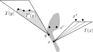
Figure 6.8: Stage 1 of the embedding in the proof of Lemma 6.20. Starting from an already embedded seed $x\in W_{A}$ we extend the embedding (in this order) to
(1) all the children $y\in W_{B}$ of $x$ in the same hub (in grey),
(2) a part $T^{\prime}(y)$ of the forest $T(y)$,
(3) all the grandchildren $x^{\prime}\in W_{A}$ of $x$ in the same hub,
(4) the forest $T(x)$ together with the bordering cut-vertices $x^{*}\in W_{A}$.

In each step we select a seed $x\in W_{A}$ already embedded in $G$ but such that none of $\mathrm{Ch}(x)$ are embedded. By (*1), or by the choice of $\phi(r)$, we have $\phi(x)\in\mathbb{H}^{\prime\prime}$. So by (6.38) we have

$$\deg_{G_{\nabla}}(\phi(x),V_{1}\setminus U)\geqslant 5(\Omega^{*})^{9}k-k.$$ (6.40)

First, we embed successively in $|W_{B}\cap\mathrm{Ch}(x)|$ steps the seeds $y\in W_{B}\cap\mathrm{Ch}(x)$ together with components $T^{\prime}(y)\subseteq T(y)$ which will be determined on the way. Suppose that in a certain step we are to embed $y\in W_{B}\cap\mathrm{Ch}(x)$ and the (to be determined) tree $T^{\prime}(y)$. Let

$$F:=\bigcup_{i=0}^{2}\mathrm{shadow}^{(i)}_{G_{\nabla}-\mathbb{H}}\left(\mathrm{ghost}(U),\frac{\eta k}{10^{5}}\right)\;,$$

where $U$ is the set of vertices used by the embedding $\phi$ in previous steps. Since $|U|\leqslant k$, Fact 4.12 gives us that $|F|\leqslant\frac{10^{10}(\Omega^{*})^{2}}{\eta^{2}}k$. We embed $y$ anywhere in $(\mathrm{N}_{G}(\phi(x))\cap V_{1})\setminus F$, cf. (6.38). Note that then (*2) holds for $y$. We use Lemma 6.19 in order to embed $T^{\prime}(y)\subseteq T(y)$ (the subtree $T^{\prime}(y)$ is determined by Lemma 6.19). Lemma 6.19 ensures that (*3) and (*4) hold and that we have $\phi(V(T^{\prime}(y)))\subseteq V(G)\setminus\mathbb{H}$.

Also, we map the vertices $x^{\prime}\in W_{A}\cap\mathrm{Ch}(y)$ to $\mathbb{H}^{\prime\prime}\setminus U$. To justify this step, employing (*2), it is enough to prove that

$$\deg(\phi(y),\mathbb{H}^{\prime\prime})\geqslant|W_{A}|\;.$$ (6.41)

Indeed, on the one hand, we have $|W_{A}|\leqslant 336/\tau$ by Definition 3.3(c). On the other hand, we have that $\phi(y)\in V_{1}$, and thus (6.39) applies. We can thus embed $x^{\prime}$ as planned, ensuring (*1), and finishing the step for $y$.

Next, we sequentially embed the components $\tilde{T}$ of $T(x)$. In the following, we describe such an embedding procedure only for an internal shrub $\tilde{T}$, with $x^{*}$ denoting the other neighbour of $\tilde{T}$ in $W_{A}$ (cf. (*1)). The case when $\tilde{T}$ is an end shrub is analogous: actually it is even easier as we do not have to worry about placing $x^{*}$ well. The actual embedding of $\tilde{T}$ together with $x^{*}$ depends on the configuration we are in. We shall slightly abuse notation by letting $U$ now denote everything embedded before the tree $\tilde{T}$.

For Configuration $\mathbf{(\diamond 2)}$, we use Lemma 6.5 for one tree, namely $\tilde{T}-x^{*}$, using the following setting: $Q_{\mathrm{L}\ref{lem:embed:greyFOREST}}:=1,\gamma_{\mathrm{L}\ref{lem:embed:greyFOREST}}:=\gamma,\zeta_{\mathrm{L}\ref{lem:embed:greyFOREST}}:=\rho^{3},H_{\mathrm{L}\ref{lem:embed:greyFOREST}}:=G_{\mathrm{exp}}$, $U_{\mathrm{L}\ref{lem:embed:greyFOREST}}:=U$, and $U^{*}_{\mathrm{L}\ref{lem:embed:greyFOREST}}:=(\mathrm{N}_{G_{\nabla}}(\phi(x))\cap V_{1})\setminus U$ (this last set is large enough by (6.40)). The child of $x$ gets embedded in $(\mathrm{N}_{G_{\nabla}}(\phi(x))\cap V_{1})\setminus U$, the vertices at odd distance from $x$ get embedded in $V_{1}$, and the vertices at even distance from $x$ get embedded in $V_{2}$. In particular, $\mathrm{Par}_{T}(x^{*})$, the parent of $x^{*}$, gets embedded in $V_{1}$. After this, we accomodate $x^{*}$ in a vertex in $\mathbb{H}^{\prime\prime}\setminus U$ which is adjacent to $\phi(\mathrm{Par}_{T}(x^{*}))$. This is possible by the same reasoning as in (6.41).

For Configuration $\mathbf{(\diamond 3)}$, we use Lemma 6.15 to embed $\tilde{T}$ with the setting $\gamma_{\mathrm{L}\ref{lem:HE3}}:=\gamma,\delta_{\mathrm{L}\ref{lem:HE3}}:=\gamma^{3}/100,U_{\mathrm{L}\ref{lem:HE3}}:=U$ and $U^{*}_{\mathrm{L}\ref{lem:HE3}}:=(\mathrm{N}_{G_{\nabla}}(\phi(x))\cap V_{1})\setminus U$ (this last set is large enough by (6.40)). Then the child of $x$ gets embedded in $(\mathrm{N}_{G_{\nabla}}(\phi(x))\cap V_{1})\setminus U$, vertices of $\tilde{T}$ of odd distance to $x$ (i.e. of even distance to the root of $\tilde{T}$) get embedded in $V_{1}\setminus U$, and vertices of even distance get embedded in $V_{2}\setminus U$. We extend the embedding by mapping $x^{*}$ to a suitable vertex in $\mathbb{H}^{\prime\prime}\setminus U$ adjacent to $\phi(\mathrm{Par}_{T}(x^{*}))$ in the same way as above.

For Configuration $\mathbf{(\diamond 4)}$, we use Lemma 6.16 to embed $\tilde{T}$ with the setting $\gamma_{\mathrm{L}\ref{lem:HE4}}:=\gamma,\delta_{\mathrm{L}\ref{lem:HE4}}:=\gamma^{4}/100,U_{\mathrm{L}\ref{lem:HE4}}:=U$ and $U^{*}_{\mathrm{L}\ref{lem:HE4}}:=(\mathrm{N}_{G_{\nabla}}(\phi(x))\cap V_{1})\setminus U$ (this last set is large enough by (6.40)). The fruit $r^{\prime}_{\mathrm{L}\ref{lem:HE4}}$ in the lemma is chosen as $\mathrm{Par}_{T}(x^{*})$. Note that this is indeed a fruit (in $\tilde{T}$) because of Definition 3.3 (i). Then the child of $x$ gets embedded in $(\mathrm{N}_{G_{\nabla}}(\phi(x))\cap V_{1})\setminus U$, the vertex $r^{\prime}_{\mathrm{L}\ref{lem:HE4}}=\mathrm{Par}_{T}(x^{*})$ gets embedded in $V_{1}\setminus U$, and the rest of $\tilde{T}$ gets embedded in $(\mathbb{E}^{\prime}\cup V_{2})\setminus U$. This allows us to extend the embedding to $x^{*}$ as above.

In Configuration $\mathbf{(\diamond 5)}$, let $\mathbf{W}\subseteq\mathbf{V}$ denote the set of those clusters, which have at least an $\frac{1}{2(\Omega^{*})^{5}}$-fraction of their vertices contained in the set $U^{\prime}:=U\cup\mathrm{shadow}_{G_{\mathrm{reg}}}(U,k/(\Omega^{*})^{3})$. We get from Fact 4.12 that $|U^{\prime}|\leqslant 2(\Omega^{*})^{4}k$, and consequently $|U^{\prime}\cup\bigcup\mathbf{W}|\leqslant 4(\Omega^{*})^{9}k$. By (6.40) we can find a vertex $v\in(\mathrm{N}_{G}(\phi(x))\cap V_{1})\setminus(U^{\prime}\cup\bigcup\mathbf{W})$.

We use the fact that $v\not\in\mathrm{shadow}_{G_{\mathrm{reg}}}(U,k/(\Omega^{*})^{3})$ together with inequality (5.28) to see that $\deg_{G_{\mathrm{reg}}}(v,V(G_{\mathrm{reg}})\setminus U)\geqslant k/(\Omega^{*})^{3}$. Now, since there are only boundedly many clusters seen from $v$ (cf. Fact 4.8), there must be a cluster $D\in\mathbf{V}$ such that

$$\deg_{G_{\mathrm{reg}}}(v,D\setminus U)\geqslant\frac{\gamma^{2}}{2\cdot(\Omega^{*})^{5}}|D|\geqslant\gamma^{3}|D|\;.$$ (6.42)

Let $C$ be the cluster containing $v$. We have $|(C\cap V_{1})\setminus U|\geqslant\frac{1}{2(\Omega^{*})^{5}}|C|\geqslant\gamma^{3}|C|$ because of (5.29) and since $C\notin\mathbf{W}$. Thus, by Fact 2.1, $\big{(}(C\cap V_{1})\setminus U,D\setminus U\big{)}$ is an $2\varepsilon^{\prime}/\gamma^{3}$-regular pair of density at least $\gamma^{2}/2$. We can therefore embed $\tilde{T}$ in this pair using the regularity method. Moreover, by (6.42), we can do so by mapping the child $z$ of $x$ to $v$. Thus the parent of $x^{*}$ (lying at even distance to $z$) will be embedded in $(C\cap V_{1})\setminus U$. We can then extend our embedding to $x^{*}$ as above.

This finishes our embedding of $T(x)$. Note that in all cases we have $\phi(x^{*})\in\mathbb{H}^{\prime\prime}$ and $\phi(V(\tilde{T}))\subseteq V(G)\setminus\mathbb{H}$, as required by (*1) and (*2).

The embedding steps of Stage 2.

For $i=1,2$, set $Z_{i}:=\bigcup_{y\in W_{B}}\mathrm{Ch}(T^{\prime}(y))\cap\bigcup\mathcal{C}_{i}(y)$.

First, we embed all the vertices $z\in Z_{2}$ in $\mathbb{H}^{\prime}$. By (*2), until now, only vertices of $W_{A}\cup Z_{2}$ are mapped to $\mathbb{H}^{\prime}$, and using (*4) and the properties (c), (k) and (l) of Definiton 3.3, we see that

$$\deg_{G}(\phi(\mathrm{Par}(z)),\mathbb{H}^{\prime}) \geqslant\frac{\eta k}{100}+\frac{k}{2}-\sum_{y\in W_{B}}v\left(T^{\prime}(y)\cup\bigcup\mathcal{C}_{1}(y)\right)$$

$$>|W_{A}|+|Z_{2}|\;.$$

So there is space for the vertex $z$ in $\mathbb{H}^{\prime}\cap\phi(\mathrm{N}_{G}(\mathrm{Par}(z)))$.

Next, we embed all the vertices $z\in Z_{1}$ in $\mathbb{H}^{\prime}$. By (*2), until now only vertices of $W_{A}\cup Z_{2}\cup Z_{1}$ are mapped to $\mathbb{H}^{\prime}$, and by (*3) we have, similarly as above,

$$\deg_{G}(\phi(\mathrm{Par}(z)),\mathbb{H}^{\prime})>|W_{A}|+|Z_{2}|+|Z_{1}|\;.$$

So $z$ can be embedded in $\mathbb{H}^{\prime}\cap\mathrm{N}_{G}(\phi(\mathrm{Par}(z)))$ as planned.

Finally, for $z\in Z_{1}\cup Z_{2}$, denote by $T_{z}$ the component of $\mathcal{C}_{1}\cup\mathcal{C}_{2}$ that contains $z$. We use Lemma 6.18 to embed the rest of the rooted tree $(T_{z},z)$. (Note that our parameters work because of (5.1).) Once all rooted trees $(T_{z},z)$ with $z\in Z_{1}\cup Z_{2}$ have been processed, we have finished Stage 2 and thus the proof of the lemma. ∎

6.5.3 Embedding in Configurations $\mathbf{(\diamond 6)}$–$\mathbf{(\diamond 10)}$

We follow the schemes outlined in Sections 6.1.2, 6.1.4, 6.1.5, and 6.1.6.

Embedding a tree $T_{\mathrm{T}\ref{thm:main}}\in\mathbf{trees}({k})$ using Configurations $\mathbf{(\diamond 6)}$, $\mathbf{(\diamond 7)}$, or $\mathbf{(\diamond 8)}$ has two parts: first the internal part of $T_{\mathrm{T}\ref{thm:main}}$ is embedded, and then this partial embedding is extended to end shrubs of $T_{\mathrm{T}\ref{thm:main}}$ as well. Lemma 6.21 (for configurations $\mathbf{(\diamond 6)}$ and $\mathbf{(\diamond 7)}$) and Lemma 6.22 (for configuration $\mathbf{(\diamond 8)}$) are used for the former part, and Lemmas 6.23 and 6.24 (depending on whether we have $\mathbf{(\heartsuit 1)}$ or $\mathbf{(\heartsuit 2)}$) for the latter. Lemma 6.25 then puts these two pieces together.

Embedding using Configurations $\mathbf{(\diamond 9)}$ and $\mathbf{(\diamond 10)}$ is resolved in Lemmas 6.26 and 6.27, respectively.

Lemma 6.21.

Suppose we are in Setting 5.1 and 5.4, and we have one of the following two configurations:

• Configuration $\mathbf{(\diamond 6)}(\delta_{6},\tilde{\varepsilon},d^{\prime},\mu,1,0)$, or

• Configuration $\mathbf{(\diamond 7)}(\delta_{7},\frac{\eta\gamma}{400},\tilde{\varepsilon},d^{\prime},\mu,1,0)$,

with $10^{5}\sqrt{\gamma}(\Omega^{*})^{2}\leqslant\delta_{6}^{4}\leqslant 1$, $10^{2}\sqrt{\gamma}(\Omega^{*})^{3}/\Lambda\leqslant\delta_{7}^{3}<\eta^{3}\gamma^{3}/10^{6}$, $d^{\prime}>10\tilde{\varepsilon}>0$, and $d^{\prime}\mu\tau k\geqslant 4\cdot 10^{3}$. Both configurations contain distinguished sets $V_{0},V_{1}\subseteq\mathbb{A}_{0}$ and $V_{2},V_{3}\subseteq\mathbb{A}_{1}$.

Suppose that $(W_{A},W_{B},\mathcal{S}_{A},\mathcal{S}_{B})$ is a $(\tau k)$-fine partition of a rooted tree $(T,r)$ of order at most $k$ such that $|W_{A}\cup W_{B}|\leqslant k^{0.1}$. Let $T^{\prime}$ be the tree induced by all the cut-vertices $W_{A}\cup W_{B}$ and all the internal shrubs.

Then there exists an embedding $\phi$ of $T^{\prime}$ such that

$$\phi(W_{A})\subseteq V_{1}\quad\phi(W_{B})\subseteq V_{0}\quad\mbox{and}\quad\phi(T^{\prime}-(W_{A}\cup W_{B}))\subseteq\mathbb{A}_{1}\;.$$

Proof.

For simplicity, let us assume that $r\in W_{A}$. The case when $r\in W_{B}$ is similar. The $(\tau k)$-fine partition $(W_{A},W_{B},\mathcal{S}_{A},\mathcal{S}_{B})$ induces a $(\tau k)$-fine partition in $T^{\prime}$. By Lemma 3.8, the tree $T^{\prime}$ has an ordered skeleton $(X_{0},X_{1},\ldots,X_{m})$ where the $X_{i}$ are either shrubs or hubs ($X_{0}$ being a hub).

Our strategy is as follows. We sequentially embed the hubs and the internal shrubs in the order given by the ordered skeleton. For embedding the hubs we use Lemma 6.5 in Preconfiguration $\mathbf{\mathbf{(exp)}}$, and Lemma 6.9 in Preconfiguration $\mathbf{\mathbf{(reg)}}$. For embedding the internal shrubs, we use Lemmas 6.13 and 6.14 if we have Configurations $\mathbf{\mathbf{(\diamond 6)}}$, and $\mathbf{\mathbf{(\diamond 7)}}$, respectively.

Throughout, $\phi$ denotes the current (partial) embedding of $(X_{0},X_{1}\ldots,X_{m})$. In consecutive steps, we extend $\phi$. We define auxiliary sets $D_{i}\subseteq V(G)$ which will serve for reserving space for the roots of the shrubs $X_{i}$. So the set $Z_{<i}:=\bigcup_{j<i}(\phi(X_{j})\cup D_{j})$ contains what is already used and what should (mainly) be avoided.

Let $W_{A,i}:=W_{A}\cap V(X_{i})$, and $W_{B,i}:=W_{B}\cap V(X_{i})$. For each $y\in W_{A,{j}}$ with $j\leqslant i$ let

$$S_{y}:=(V_{2}\cap\mathrm{N}_{G}(\phi(y)))\setminus Z_{<i},$$

except if the latter set has size $>k$, in that case we choose a subset of size $k$. This is a target set for the roots of shrubs adjacent to $y$.

Also, in the case $X_{i}$ is a shrub, we write $r_{i}$ for its root, and $f_{i}$ for the only other vertex neighbouring $W_{A}\cup W_{B}$. Note that $f_{i}$ is a fruit of $(X_{i},r_{i})$.

The value $h=6$ or $h=7$ indicates whether we have configuration $\mathbf{\mathbf{(\diamond 6)}}$ or $\mathbf{\mathbf{(\diamond 7)}}$. Define

$$F_{i}:=\mathrm{shadow}_{G-\mathbb{H}}\left(Z_{<i},\frac{\delta_{h}k}{4}\right)\cup Z_{<i}\;.$$ (6.43)

Define $U_{i}:=F_{i}$ if we have Preconfiguration $\mathbf{\mathbf{(exp)}}$ (note that in that case we have Configuration $\mathbf{\mathbf{(\diamond 6)}}$). To define $U_{i}$ in case of Preconfiguration $\mathbf{\mathbf{(reg)}}$ we make use of the super-regular pairs $(Q^{(j)}_{0},Q^{(j)}_{1})$ ($j\in\mathcal{Y}$). Set

$$U_{i}:=F_{i}\cup\bigcup\left\{Q^{(j)}_{1}\>:\>j\in\mathcal{Y},|Q^{(j)}_{1}\cap F_{i}|\geqslant\frac{|Q^{(j)}_{1}|}{2}\right\}\;.$$ (6.44)

In either case, we have $|U_{i}|\leqslant 2|F_{i}|$.

Finally, set

$$W_{i} :=\mathrm{shadow}_{G-\mathbb{H}}\left(U_{i},\frac{\delta_{h}k}{2}\right)\cup Z_{<i}\;.$$ (6.45)

We will now show how to embed successively all $X_{i}$. At each step $i$, our embedding $\phi$ will have the following properties:

1. $\phi(W_{A,i})\subseteq V_{1}\setminus F_{i}$ and $\phi(W_{B,i})\subseteq V_{0}$,

2. for each $y\in W_{A,{j}}$ with $j\leqslant i$ we have $|S_{y}\cap\phi(X_{i})|\leqslant|S_{y}\cap D_{i}|+k^{3/4}$,

3. $|Z_{<i+1}|\leqslant 2k$,

4. $D_{i}\subseteq\mathbb{A}_{1}\setminus(\phi(X_{i})\cup Z_{<i})$,

5. $\phi(X_{i}-r_{i})$ is disjoint from $\bigcup_{j<i}D_{j}$,

6. $\phi(f_{i})\in V_{2}\setminus W_{i}$ if $X_{i}$ is a shrub,

7. $\phi(X_{i})\subseteq\mathbb{A}_{1}$ if $X_{i}$ is a shrub.

(We remark that since $r_{i}$ is not defined for hubs $X_{i}$, condition (e) means that $\phi(X_{i})$ is disjoint from $\bigcup_{j<i}\cup D_{j}$ for hubs $X_{i}$.)

It is clear that conditions (a) and (g) ensure that in step $m$ we have found the desired embedding for $T^{\prime}$.

Before we show how to embed each $X_{i}$ fulfilling the properties above, let us quickly derive a useful bound. By Fact 4.12 and (c), we have that $|F_{i}|\leqslant\frac{9\Omega^{*}}{\delta_{h}}k$ for all $i\leqslant m$. Thus, using $|U_{i}|\leqslant 2|F_{i}|$ and again Fact 4.12 and (c), we get that

$$|W_{i}|\leqslant\frac{38(\Omega^{*})^{2}}{\delta_{h}^{2}}k\;.$$ (6.46)

Now suppose we are at step $i$ with $0\leqslant i\leqslant m$. That is, we have already embedded all $X_{j}$ with $j<i$, and are about to embed $X_{i}$.

First assume that $X_{i}$ is a hub. Note that if $i\neq 0$, then there is exactly one fruit $f_{\ell}$ with $\ell<i$ which neighbours $X_{i}$. Set $N_{i}:=\mathrm{N}_{G}(\phi(f_{\ell}))$ in this case, and let $N_{i}:=V(G)$ for $i=0$. We distinguish between the two preconfigurations we might be in.

Suppose first we are in Preconfiguration $\mathbf{\mathbf{(exp)}}$. Recall that then we are in Configuration $\mathbf{(\diamond 6)}$.

We use Lemma 6.5 to embed the single tree $X_{i}$ with the following setting: $\ell_{\mathrm{L}\ref{lem:embed:greyFOREST}}:=1$, $V_{1,{\mathrm{L}\ref{lem:embed:greyFOREST}}}:=V_{1}$, $V_{2,{\mathrm{L}\ref{lem:embed:greyFOREST}}}:=V_{0}$, $U^{*}_{\mathrm{L}\ref{lem:embed:greyFOREST}}:=(N_{i}\cap V_{1})\setminus U_{i}=(N_{i}\cap V_{1})\setminus F_{i}$, $U_{\mathrm{L}\ref{lem:embed:greyFOREST}}:=U_{i}=F_{i}$, $Q_{\mathrm{L}\ref{lem:embed:greyFOREST}}:=\frac{18\Omega^{*}}{\delta_{6}}$, $\zeta_{\mathrm{L}\ref{lem:embed:greyFOREST}}:=\delta_{6}$, and $\gamma_{\mathrm{L}\ref{lem:embed:greyFOREST}}:=\gamma$. Note that $U^{*}_{\mathrm{L}\ref{lem:embed:greyFOREST}}$ is large enough by (f) for $\ell$ and by (5.38) and (5.42), respectively. Lemma 6.5 gives an embedding of the tree $X_{i}$ such that $\phi(V_{\mathrm{even}}(X_{i}))\subseteq V_{1}\setminus F_{i}$ and $\phi(V_{\mathrm{odd}}(X_{i}))\subseteq V_{0}\setminus F_{i}$ , which maps the root of $X_{i}$ to the neighbourhood of its parent’s image. Note that this ensures (a) and (e) for step $i$, and setting $D_{i}:=\emptyset$ we also ensure (c) and (d). Property (b) holds since $V_{2}\cap\phi(X_{i})=\emptyset$. Since $X_{i}$ is a hub, (f) and (g) are empty.

Suppose now we are in Preconfiguration $\mathbf{\mathbf{(reg)}}$. Then let $j\in\mathcal{Y}$ be such that $(N_{i}\cap Q_{1}^{(j)})\setminus U_{i}\neq\emptyset$. Such an index $j$ exists by (f) for $\ell$ and by (5.38) and (5.42), respectively, if $i\neq 0$, and trivially if $i=0$. We shall use Lemma 6.9 to embed $X_{i}$ in $(Q^{(j)}_{0},Q^{(j)}_{1})$. More precisely, we use Lemma 6.9 with $A_{\mathrm{L}\ref{lem:embed:superregular}}:=Q^{(j)}_{1}$, $B_{\mathrm{L}\ref{lem:embed:superregular}}:=Q^{(j)}_{0}$, $\varepsilon_{\mathrm{L}\ref{lem:embed:superregular}}:=\tilde{\varepsilon}$, $d_{\mathrm{L}\ref{lem:embed:superregular}}:=d^{\prime}$, $\ell_{\mathrm{L}\ref{lem:embed:superregular}}:=\mu k$, $U_{A}:=U_{i}\cap A$, $U_{B}:=\phi(W_{B,<i})\cap B$ (then $|U_{A}|\leqslant|A|/2$ by the definition of $U_{i}$ and the choice of $j$).

Lemma 6.9 yields a $(V_{\mathrm{even}}(X_{i})\hookrightarrow V_{1}\setminus F_{i},V_{\mathrm{odd}}(X_{i})\hookrightarrow V_{0})$-embedding of $X_{i}$, which maps the root of $X_{i}$ to the neighbourhood of its parent’s image. Setting $D_{i}:=\emptyset$, we have (a)–(g).

So let us now assume that $X_{i}$ is a shrub. The parent $y$ of the root $r_{i}$ of $X_{i}$ lies in $W_{A,\ell}$ for some $\ell<i$. By (a) for $\ell$, we mapped $y$ to a vertex $\phi(y)\in V_{1}\setminus F_{\ell}$. As $\deg_{G}(\phi(y),V_{2})\geqslant\delta_{h}k$ (by (5.37) and (5.41), respectively), and since $\phi(y)\notin F_{\ell}$, we have

$$|S_{y}|\geqslant\frac{3\delta_{h}k}{4}.$$ (6.47)

Using (b) for all $j$ with $\ell\leqslant j<i$, and using that the sets $D_{j}$ are pairwise disjoint by (d), we see that

$$|S_{y}\cap\phi(X_{0}\cup\ldots\cup X_{i-1})|=|S_{y}\cap\phi(X_{\ell}\cup\ldots\cup X_{i-1})|\leqslant|S_{y}\cap\bigcup_{\ell\leqslant j<i}D_{j}|+m\cdot k^{3/4}\leqslant|S_{y}\cap\bigcup_{0\leqslant j<i}D_{j}|+m\cdot k^{3/4}.$$

Therefore, and as by (d) and (e), the sets $\phi(X_{0}\cup\ldots X_{i-1})$ and $\bigcup_{0\leqslant j<i}D_{j}$ are disjoint except for the at most $m\leqslant|W_{A}\cup W_{B}|\leqslant k^{0.1}$ roots $r_{j}$ of shrubs $X_{j}$, and since $k\gg 1$, we have

$$|S_{y}|\geqslant|S_{y}\cap\phi(X_{0}\cup\ldots\cup X_{i-1})|+|S_{y}\cap\bigcup_{0\leqslant j<i}D_{j}|-m\geqslant 2|S_{y}\cap\phi(X_{0}\cup\ldots\cup X_{i-1})|-k^{0.9}.$$

Thus,

$$|S_{y}\setminus\phi(X_{0}\cup\ldots\cup X_{i-1})|\geqslant\frac{|S_{y}|-k^{0.9}}{2}\overset{\eqref{cerropochoco}}{\geqslant}\frac{3\delta_{h}k}{8}-\frac{k^{0.9}}{2}>\frac{\delta_{h}k}{3}\;.$$

So for $U^{*}:=S_{y}\setminus\phi(X_{0}\cup\ldots\cup X_{i-1})$ we have that $|U^{*}|\geqslant\frac{\delta_{h}k}{3}$. If we have Configuration $\mathbf{(\diamond 6)}$ or $\mathbf{(\diamond 7)}$ we use Lemma 6.13 or 6.14, respectively, with input $U_{\mathrm{L}\ref{lem:embedStoch:DIAMOND6}-\ref{lem:embedStoch:DIAMOND7}}:=W_{i}$, $U^{*}_{\mathrm{L}\ref{lem:embedStoch:DIAMOND6}-\ref{lem:embedStoch:DIAMOND7}}:=U^{*}$, $L_{\mathrm{L}\ref{lem:embedStoch:DIAMOND6}-\ref{lem:embedStoch:DIAMOND7}}:=|W_{A,{i}}|$, $\gamma_{\mathrm{L}\ref{lem:embedStoch:DIAMOND6}-\ref{lem:embedStoch:DIAMOND7}}:=\gamma$, the family $\{P_{t}\}_{\mathrm{L}\ref{lem:embedStoch:DIAMOND6}-\ref{lem:embedStoch:DIAMOND7}}:=\{S_{y}\}_{y\in W_{A,{j}},j<i}$, and the rooted tree $(X_{i},r_{i})$ with fruit $f_{i}$. Further, for Configuration $\mathbf{(\diamond 6)}$, set $\delta_{\mathrm{L}\ref{lem:embedStoch:DIAMOND6}}:=\delta_{6}$, $V_{2,{\mathrm{L}\ref{lem:embedStoch:DIAMOND6}}}:=V_{2}$ and $V_{3,{\mathrm{L}\ref{lem:embedStoch:DIAMOND6}}}:=V_{3}$ and for Configuration $\mathbf{(\diamond 7)}$, set $\delta_{\mathrm{L}\ref{lem:embedStoch:DIAMOND7}}:=\delta_{7}$, $\ell_{{\mathrm{L}\ref{lem:embedStoch:DIAMOND7}}}:=1$, $Y_{1,{\mathrm{L}\ref{lem:embedStoch:DIAMOND7}}}:=V_{2}$ and $Y_{2,{\mathrm{L}\ref{lem:embedStoch:DIAMOND7}}}:=V_{3}$. The output of Lemma 6.13 or 6.14, respectively, is the extension of our embedding $\phi$ to $X_{i}$, and a set $D_{i}:=C_{\mathrm{L}\ref{lem:embedStoch:DIAMOND6}-\ref{lem:embedStoch:DIAMOND7}}\subseteq(V_{2}\cup V_{3})\setminus(W_{i}\cup\phi(X_{i}))$ for which property (a) (which is empty) and properties (b)–(g) hold. ∎

Lemma 6.22.

Suppose we are in Setting 5.1 and 5.4 and suppose further we have Configuration $\mathbf{(\diamond 8)}(\delta,\frac{\eta\gamma}{400},\varepsilon_{1},\varepsilon_{2},d_{1},d_{2},\mu_{1},\mu_{2},h_{1},0)$, with $2\cdot 10^{5}(\Omega^{*})^{6}/\Lambda\leqslant\delta^{6}$, $\delta<\gamma^{2}\eta^{4}/(10^{16}(\Omega^{*})^{2})$, $d_{2}>10\varepsilon_{2}>0$, $d_{2}\mu_{2}\tau k\geqslant 4\cdot 10^{3}$, and $\max\{\varepsilon_{1},\tau/\mu_{1}\}\leqslant\eta^{2}\gamma^{2}d_{1}/(10^{10}(\Omega^{*})^{3})$. Recall that we have distinguished sets $V_{0},\ldots,V_{4}$ and a regularized matching $\mathcal{N}$.

Let $(W_{A},W_{B},\mathcal{S}_{A},\mathcal{S}_{B})$ be a $(\tau k)$-fine partition of a rooted tree $(T,r)$ of order at most $k$. Let $T^{\prime}$ be the tree induced by all the cut-vertices $W_{A}\cup W_{B}$ and all the internal shrubs. Suppose that

$$v(T^{\prime})<h_{1}-\frac{\eta^{2}k}{10^{5}}\;.$$ (6.48)

Then there exists an embedding $\phi$ of $T^{\prime}$ such that $\phi(W_{A})\subseteq V_{1}$, $\phi(W_{B})\subseteq V_{0}$, and $\phi(T^{\prime})\subseteq\mathbb{A}_{0}\cup\mathbb{A}_{1}$.

Proof.

We assume that $r\in W_{A}$. The case when $r\in W_{B}$ is similar.

Let $\mathcal{K}$ be the set of all hubs of the $(\tau k)$-fine partition $(W_{A},W_{B},\mathcal{S}_{A},\mathcal{S}_{B})$ of $T$. For each such hub $K\in\mathcal{K}$ set $Y_{K}:=K\cup\mathrm{Ch}_{T^{\prime}}(K)$. We call the subgraphs $Y_{K}$ extended hubs. Set $\mathcal{Y}:=\{Y_{K}:K\in\mathcal{K}\}$ and $W_{C}:=V(\bigcup\mathcal{Y}\setminus\bigcup\mathcal{K})$. Since $W_{C}\subseteq V(T^{\prime})$, we clearly have that $|W_{C}|\leqslant|W_{A}\cup W_{B}|$.

Note that the forest $T^{\prime}-\bigcup\mathcal{Y}$ consists of the set $\mathcal{P}$ of peripheral subshrubs of internal shrubs of $(W_{A},W_{B},\mathcal{S}_{A},\mathcal{S}_{B})$, and the set $\mathcal{S}$ of principal subshrubs of internal shrubs of $(W_{A},W_{B},\mathcal{S}_{A},\mathcal{S}_{B})$. It is not difficult to observe that there is a sequence $(X_{0},X_{1},\ldots,X_{m})$ such that $X_{i}=(M_{i},Y_{i},\mathcal{P}_{i})$, $M_{i}\in\mathcal{S}$ and $\mathcal{P}_{i}\subseteq\mathcal{P}$ for each $i\leqslant m$, and such that we have the following.

1. $M_{0}=\emptyset$ and $Y_{0}$ contains $r$.

2. $\mathcal{P}_{i}$ are exactly those peripheral subshrubs whose parents lie in $Y_{i}$.

3. The parent $f_{i}$ of $Y_{i}$ lies in $M_{i}$ (unless $i=0$).

4. The parent $r_{i}$ of $M_{i}$ lies in some $Y_{j}$ with $j<i$ (unless $i=0$),

5. $\bigcup_{i\leqslant m}V(M_{i}\cup Y_{i}\cup\bigcup\mathcal{P}_{i})=V(T^{\prime})$.

See Figure 6.9 for an illustration.

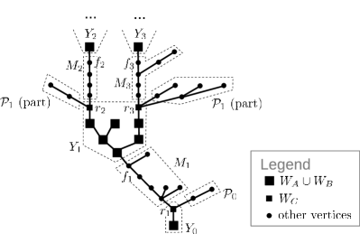
Figure 6.9: An example of a sequence $(X_{0},X_{1},X_{2},X_{3},\ldots)$ in Lemma 6.22.

We now successively embed the elements of $X_{i}$, except possibly for a part of the subshrubs in $\mathcal{P}_{i}$. The omitted peripheral subshrubs will be embedded at the very end, after having completed the inductive procedure we are about to describe now.

We shall make use of the following lemmas: Lemma 6.9 (for embedding hubs), Lemmas 6.10 and 6.7 (for embedding peripheral subshrubs in $\mathcal{N}$), Lemma 6.14 (for embedding principal subshrubs in $V_{3}\cup V_{4}$).

Throughout, $\phi$ denotes the current (partial) embedding of $T^{\prime}$. In each step $i$ we embed $M_{i}\cup Y_{i}$ and a subset of $\mathcal{P}_{i}$, and denote by $\phi(X_{i})$ the image of these sets (as far as it is defined). We also define an auxiliary set $D_{i}\subseteq V(G)$ which will ensure that there is enough space for the roots of the subshrubs $M_{\ell}$ with $\ell>i$. Set

$$Z_{<i}:=\bigcup_{j<i}(\phi(X_{j})\cup D_{j}).$$

Our plan for embedding the various parts of $X_{i}$ is depicted in Figure 6.10, which is a refined version of Figure 6.5.

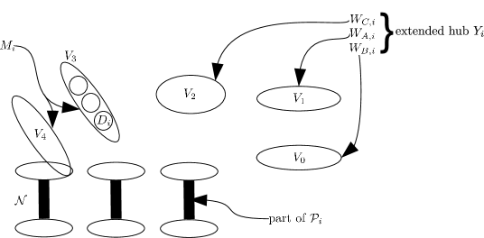
Figure 6.10: Embedding a part of the internal tree in Lemma 6.22.

Let $W_{O,i}:=W_{O}\cap V(Y_{i})$ for $O=A,B,C$. For each $y\in W_{C,{i}}$ let

$$S_{y}:=(V_{3}\cap\mathrm{N}_{G}(\phi(y)))\setminus Z_{<i},$$

except if this set has size more than $k$, in which case we choose any subset of size $k$. Similar as in the preceding lemma, this is a target set for the roots of the principal subshrub adjacent to $y$.

Fix a matching involution $\mathfrak{d}$ for $\mathcal{N}$, and for $\ell=1,2$ define

$$F^{(\ell)}_{i}:=Z_{<i}\cup\mathrm{shadow}^{(\ell)}_{G-\mathbb{H}}\left(\mathrm{ghost}_{\mathfrak{d}}(Z_{<i}),\frac{\delta k}{8}\right)\;.$$ (6.49)

We use the super-regular pairs $(Q^{(j)}_{0},Q^{(j)}_{1})$ ($j\in\mathcal{Y}$) to define

$$U_{i}:=F^{(2)}_{i}\cup\bigcup\left\{Q^{(j)}_{1}\>:\>j\in\mathcal{Y},|Q^{(j)}_{1}\cap F^{(2)}_{i}|\geqslant\frac{|Q^{(j)}_{1}|}{2}\right\}\;.$$ (6.50)

We have

$$|U_{i}|\leqslant 2|F^{(2)}_{i}|.$$ (6.51)

Finally, for $\ell=1,2$ set

$$W^{(\ell)}_{i} :=\mathrm{shadow}^{(\ell)}_{G-\mathbb{H}}\left(U_{i},\frac{\delta k}{2}\right)\;.$$ (6.52)

We will now show how to define successively our embedding. At each step $i$, the embedding $\phi$ will be defined for $M_{i}\cup Y_{i}$ and a subset of $\mathcal{P}_{i}$, and it will have the following properties:

1. $\phi(W_{A,i})\subseteq V_{1}\setminus F^{(2)}_{i}$ and $\phi(W_{B,i})\subseteq V_{0}$,

2. $\phi(W_{C,i})\subseteq V_{2}\setminus F^{(1)}_{i}$,

3. $\phi(f_{i})\in V_{2}\setminus(F^{(1)}_{i}\cup W^{(1)}_{i})$,

4. for each $y\in W_{C,{j}}$ with $j\leqslant i$ we have $|S_{y}\cap\phi(X_{i})|\leqslant|S_{y}\cap D_{i}|+2k^{3/4}$,

5. $|Z_{<i+1}|\leqslant 2k$,

6. $D_{i}\subseteq V_{3}\setminus(\phi(X_{i})\cup Z_{<i})$,

7. $\phi(X_{i}\setminus(V(M_{i})\cap\mathrm{Ch}(W_{C})))$ is disjoint from $\bigcup_{j<i}D_{j}$,

8. $\phi(X_{i})\subseteq\mathbb{A}_{1}\cup\phi(Y_{i}\cup f_{i})$,

9. if $P\in\mathcal{P}_{i}$ is not embedded in step $i$ then for its parent $w\in W_{C}$ we have that $\deg_{G_{\mathcal{D}}}(\phi(w),V_{3})\geqslant h_{1}-|\phi(X_{i})\cap V(\mathcal{N})|-\frac{\eta^{2}k}{10^{6}}$.

Note that for (h), since $f_{0}$ is not defined, we assume $\phi(f_{0})=\emptyset$.

Before continuing, let us remark that (h) together with (f) implies that at each step $i$ we have

$$\left|Z_{<i}\cap\mathbb{A}_{0}\right|\leqslant 3\cdot(|W_{A}|+|W_{B}|)\overset{\mbox{\tiny{D\ref{ellfine}\eqref{few}}}}{\leqslant}\frac{2016}{\tau}<\frac{\delta k}{8}\;.$$ (6.53)

Also note that by Fact 4.12 and by (e), we have

$$|F^{(2)}_{i}|\leqslant\frac{65(\Omega^{*})^{2}}{\delta^{2}}k\;,$$ (6.54)

and

$$|W^{(2)}_{i}|\leqslant\frac{520(\Omega^{*})^{4}}{\delta^{4}}k\;.$$ (6.55)

By (b) and by (5.47) we have that $|S_{y}|\geqslant\frac{7\delta k}{8}$. Now, using (d), (f) and (g), we can calculate similarly as in the previous lemma that at each step $i$ we have

$$\left|S_{y}\setminus\bigcup_{\ell\leqslant i}\phi(X_{\ell})\right|\geqslant\frac{3\delta k}{8}\;.$$ (6.56)

Now assume we are at step $i$ of the inductive procedure, that is, we have already dealt with $X_{0},\ldots,X_{i-1}$ and wish to embed (parts of) $X_{i}$.

We start with embedding $M_{i}$, except if $i=0$, when we go directly to embedding $Y_{0}$. We shall embed $M_{i}$ in $V_{3}\cup V_{4}$, except for the fruit $f_{i}$, which will be mapped to $V_{2}$. The embedding has three stages. First we embed $M_{i}-M_{i}(\uparrow f_{i})$, then we embed $f_{i}$, and finally we embed the forest $M_{i}(\uparrow f_{i})-f_{i}$. The embedding of $M_{i}-M_{i}(\uparrow f_{i})$ is an application of Lemma 6.14 analogous to the case of Configuration $\mathbf{(\diamond 7)}$ in the previous Lemma 6.21. That is, set $Y_{1,{\mathrm{L}\ref{lem:embedStoch:DIAMOND7}}}:=V_{3}$, $Y_{2,{\mathrm{L}\ref{lem:embedStoch:DIAMOND7}}}:=V_{4}$, let

$$U_{\mathrm{L}\ref{lem:embedStoch:DIAMOND7}}^{*}:=S_{r_{i}}\setminus\bigcup_{\ell<i}\phi(X_{i}),$$

where $r_{i}$ lies in $W_{C}$ by (IV), and

$$U_{\mathrm{L}\ref{lem:embedStoch:DIAMOND7}}:=F^{(2)}_{i}\cup W^{(2)}_{i}\;.$$

Note that

$$|U_{\mathrm{L}\ref{lem:embedStoch:DIAMOND7}}|\leqslant\frac{10^{3}(\Omega^{*})^{4}}{\delta^{4}}k\leqslant\frac{\delta\Lambda}{2\Omega^{*}}k,$$

and by (6.56) (which we use for $i-1$), also

$$|U^{*}_{\mathrm{L}\ref{lem:embedStoch:DIAMOND7}}|\geqslant\frac{3\delta k}{8}.$$

The family $\{P_{1},\ldots,P_{L}\}_{\mathrm{L}\ref{lem:embedStoch:DIAMOND7}}$ is the same as $\{S_{y}\}_{y\in\bigcup_{j<i}W_{C,j}}$. There is only one tree to be embedded, namely $M_{i}-M_{i}(\uparrow f_{i})$. It is not difficult to check that all the conditions of Lemma 6.14 are fulfilled. Lemma 6.14 gives an embedding of $M_{i}-M_{i}(\uparrow f_{i})$ in $V_{3}\cup V_{4}\subseteq\mathbb{A}_{1}$ with the property that $\mathrm{Par}(f_{i})$, the parent of the fruit $f_{i}$, is mapped to $V_{3}\setminus(F^{(2)}_{i}\cup W^{(2)}_{i})$. The lemma further gives a set $D^{\prime}:=C_{\mathrm{L}\ref{lem:embedStoch:DIAMOND7}}$ of size $v(M_{i}-M_{i}(\uparrow f_{i}))$ such that

$$|S_{y}\cap\phi(M_{i}-M_{i}(\uparrow f_{i}))|\leqslant|S_{y}\cap D^{\prime}|+k^{0.75}$$

for each $y\in\bigcup_{j<i}W_{C,j}$.

Using the degree condition (5.48) we can embed $f_{i}$ to

$$V_{2}\setminus(F^{(1)}_{i}\cup W^{(1)}_{i})$$

(recall that (6.53) asserts that only very little space in $V_{2}$ is occupied). This ensures (c) for $i$.

To embed $M_{i}(\uparrow f_{i})-f_{i}$ we use again Lemma 6.14. The parameters are this time $Y_{1,{\mathrm{L}\ref{lem:embedStoch:DIAMOND7}}}:=V_{3}$, $Y_{2,,{\mathrm{L}\ref{lem:embedStoch:DIAMOND7}}}:=V_{4}$,

$$U_{\mathrm{L}\ref{lem:embedStoch:DIAMOND7}}^{*} :=(\mathrm{N}_{G}(\phi(f_{i}))\cap V_{3})\setminus(Z_{<i}\cup\phi(M_{i}-M_{i}(\uparrow f_{i})))\;\mbox{, and}$$

$$U_{\mathrm{L}\ref{lem:embedStoch:DIAMOND7}} :=Z_{<i}\cup\phi(M_{i}-M_{i}(\uparrow f_{i}))\cup D^{\prime}\;.$$

Note that $|U_{\mathrm{L}\ref{lem:embedStoch:DIAMOND7}}^{*}|\geqslant\frac{\delta k}{4}$ by (5.47), by the fact that $\phi(f_{i})\not\in W^{(1)}_{i}$, and as $v(T_{i})+i<\delta k/8$. The family $\{P_{1},\ldots,P_{L}\}_{\mathrm{L}\ref{lem:embedStoch:DIAMOND7}}$ is $\{S_{y}\}_{y\in\bigcup_{j<i}W_{C,j}}$. The trees to be embedded are the components of $M_{i}(\uparrow f_{i})-f_{i}$ rooted at the children of $f_{i}$. All the conditions of Lemma 6.14 are fulfilled. The lemma provides an embedding in $V_{3}\cup V_{4}\subseteq\mathbb{A}_{1}$. It further gives a set $D^{\prime\prime}:=C_{\mathrm{L}\ref{lem:embedStoch:DIAMOND7}}$ of size $v(M_{i}(\uparrow f_{i}))-1$ such that

$$|S_{y}\cap\phi(M_{i}(\uparrow f_{i})-f_{i})|\leqslant|S_{y}\cap D^{\prime\prime}|+k^{0.75}$$

for each $y\in\bigcup_{j<i}W_{C,j}$. Then $D_{i}:=V_{3}\cap(D^{\prime}\cup D^{\prime\prime})$ is such that for each $y\in\bigcup_{j<i}W_{C,j}$,

$$|S_{y}\cap\phi(M_{i})|\leqslant|S_{y}\cap D_{i}|+2k^{0.75}\;,$$ (6.57)

as $S_{y}\subseteq V_{3}$ and $\phi(f_{i})\notin V_{3}$. Note that this choice of $D_{i}$ also ensures (e) for $i$, and we have by the choices of $U_{\mathrm{L}\ref{lem:embedStoch:DIAMOND7}}^{*}$ and $U_{\mathrm{L}\ref{lem:embedStoch:DIAMOND7}}$ in both applications of Lemma 6.14 that

$$D_{i}\subseteq V_{3}\setminus(\phi(M_{i})\cup Z_{<i})\quad\text{ and }\quad\phi(X_{i}\setminus(V(M_{i})\cap\mathrm{Ch}(W_{C})))\cap\bigcup_{j<i}D_{j}=\emptyset.\,$$ (6.58)

We now turn to embedding $Y_{i}$. Our plan is to use first Lemma 6.9 to embed $Y_{i}\setminus W_{C}$ in $(Q^{(j)}_{0},Q^{(j)}_{1})$ for an appropriate index $j$. After that, we shall show how to embed $W_{C,i}$.

If $i=0$ then take an arbitrary $j\in\mathcal{Y}$. Otherwise note that by (III), the parent $f_{i}$ of the root of $Y_{i}$ lies in $M_{i}$. Note that $f_{i}$ is a fruit in $M_{i}$. Let $j\in\mathcal{Y}$ be such that $(\mathrm{N}_{G}(\phi(f_{i}))\cap Q_{1}^{(j)})\setminus U_{i}\neq\emptyset$. Such an index $j$ exists by (5.46) and the fact that $\phi(f_{i})\not\in W^{(1)}_{i}$ by (c) for $i$.

We use Lemma 6.9 with $A_{\mathrm{L}\ref{lem:embed:superregular}}:=Q^{(j)}_{1}$, $B_{\mathrm{L}\ref{lem:embed:superregular}}:=Q^{(j)}_{0}$, $\varepsilon_{\mathrm{L}\ref{lem:embed:superregular}}:=\varepsilon_{2}$, $d_{\mathrm{L}\ref{lem:embed:superregular}}:=d_{2}$, $\ell_{\mathrm{L}\ref{lem:embed:superregular}}:=\mu_{2}k$, $U_{A}:=U_{i}\cap A_{\mathrm{L}\ref{lem:embed:superregular}}$, $U_{B}:=Z_{<i}\cap B_{\mathrm{L}\ref{lem:embed:superregular}}$. By the choice of $j$ and the definition of $U_{i}$, we find that $U_{A}$ is small enough, and using (6.53) we see that $U_{B}$ is also small enough. Lemma 6.9 yields a $(V_{\mathrm{even}}(Y_{i}-W_{C})\hookrightarrow V_{1}\setminus F^{(2)}_{i},V_{\mathrm{odd}}(Y_{i}-W_{C})\hookrightarrow V_{0})$-embedding of $Y_{i}-W_{C}$. We clearly see condition (a) satisfied for $i$.

We now embed successively the vertices of the set $W_{C,i}=\{w_{\ell}:\ell=1,\ldots,|W_{C,i}|\}$. By the definition of the set $W_{C}$, we know that the parent $x$ of $w_{\ell}$ lies in $W_{A,i}$. Combining (5.45) with the fact that $\phi(x)\in V_{1}\setminus F^{(2)}_{i}$ by (a) for $i$, we have that

$$\left|\mathrm{N}_{G}\left(\phi(x),V_{2}\setminus(F^{(1)}_{i}\setminus Z_{<i})\right)\right|\geqslant\frac{7\delta k}{8}\;.$$

Thus by (6.53) and since $V_{2}\subseteq\mathbb{A}_{0}$, we can accommodate $w_{\ell}$ in $V_{2}\setminus F^{(1)}_{i}$. This is as desired for (b) in step $i$.

We now turn to $\mathcal{P}_{i}$. We will embed a subset of these peripheral subshrubs in $\mathcal{N}$. This procedure is divided into two stages. First we shall embed as many subshrubs as possible in $\mathcal{N}$ in a balanced way, with the help of Lemma 6.10. When it is no longer possible to embed any subshrub in a balanced way in $\mathcal{N}$, we embed in $\mathcal{N}$ as many of the leftover subshrubs as possible, in an unbalanced way. For this part of the embedding we use Lemma 6.7.

By (II) all the parents of the subshrubs in $\mathcal{P}_{i}$ lie in $W_{C,i}$. For $w_{\ell}\in W_{C,i}$, let $\mathcal{P}_{i,\ell}$ denote the set of all subshrubs in $\mathcal{P}_{i}$ adjacent to $w_{\ell}$. In the first stage, we shall embed, successively for $j=1,\ldots,|W_{C,i}|$, either all or none of $\mathcal{P}_{i,j}$ in a balanced way in $\mathcal{N}$. Assume inductively that

$$\phi\Big{(}\bigcup_{p<j}\mathcal{P}_{i,p}\Big{)}\mbox{ is $(\tau k)$-balanced with respect to $\mathcal{N}$.}$$ (6.59)

Construct a regularized matching $\mathcal{N}_{j}$ absorbed by $\mathcal{N}$ as follows. Let $\mathcal{N}_{j}:=\{(X_{1}^{\prime},X_{2}^{\prime})\>:\>(X_{1},X_{2})\in\mathcal{N}\}$, where for $(X_{1},X_{2})\in\mathcal{N}$ we define $(X^{\prime}_{1},X_{2}^{\prime})$ as the maximal balanced unoccupied subpair seen from $\phi(w_{j})$, i.e., for $b=1,2$, we take

$$X^{\prime}_{b}\subseteq\left(X_{b}\cap\mathrm{N}_{G_{\mathrm{reg}}}(\phi(w_{j})\right)\setminus\left(\phi(\bigcup_{p<j}\mathcal{P}_{i,p})\cup\bigcup_{\ell<i}\phi(X_{\ell})\right)$$

maximal subject to $|X^{\prime}_{1}|=|X^{\prime}_{2}|$. If $|V(\mathcal{N}_{j})|\geqslant\frac{\eta^{2}k}{10^{7}\Omega^{*}}$ then we shall embed $\mathcal{P}_{i,j}$, otherwise we do not embed $\mathcal{P}_{i,j}$ in this step. So assume we decided to embed $\mathcal{P}_{i,j}$. Recall that the total order of the subshrubs in this set is at most $\tau k$. Using the same argument as for Claim 6.19.1 we have

$$\left|\bigcup\{X\cup Y\>:\>(X,Y)\in\mathcal{N},\deg_{G_{\mathcal{D}}}(\phi(w_{j}),X\cup Y)>0\}\right|\leqslant\frac{4(\Omega^{*})^{2}}{\gamma^{2}}k\;.$$

Thus, there exists a subpair $(X_{1}^{\prime},X_{2}^{\prime})\in\mathcal{N}_{j}$ of some $(X_{1},X_{2})\in\mathcal{N}$ with

$$\frac{|X_{1}^{\prime}|}{|X_{1}|}\geqslant\frac{\tfrac{\eta^{2}}{10^{7}\Omega^{*}}k}{\tfrac{4(\Omega^{*})^{2}}{\gamma^{2}}k}\geqslant\frac{\gamma^{2}\eta^{2}}{10^{8}(\Omega^{*})^{3}}\;.$$ (6.60)

In particular, $(X_{1}^{\prime},X_{2}^{\prime})$ forms a $\frac{2\cdot 10^{8}\varepsilon_{1}(\Omega^{*})^{3}}{\gamma^{2}\eta^{2}}$-regular pair of density at least $d_{1}/2$ by Fact 2.1. We use Lemma 6.10 to embed $\mathcal{P}_{i,j}$ in $\mathcal{M}_{\mathrm{L}\ref{lem:embed:BALANCED}}:=\{(X_{1}^{\prime},X_{2}^{\prime})\}$. The family $\{f_{CD}\}_{\mathrm{L}\ref{lem:embed:BALANCED}}$ consists of a single number $f_{(X_{1}^{\prime},X_{2}^{\prime})}$ which is the discrepancy of $\bigcup_{p<j}\phi(\mathcal{P}_{i,p})$ with respect to $(X_{1},X_{2})$. This guarantees that (6.59) is preserved. This finishes the $j$-th step. We repeat this step until $j=|W_{C,i}|$, then we go to the next stage.

Denote by $\mathcal{Q}_{i}$ the set of all $P\in\mathcal{P}_{i}$ that have not been embedded in the first stage. Note that for each $Q\in\mathcal{Q}_{i}$, with $Q\in\mathcal{P}_{i,j}$, say, and for each $(X_{1},X_{2})\in\mathcal{N}$ there is a $b_{(X_{1},X_{2})}\in\{1,2\}$ such that for

$$O_{j}:=\bigcup_{(X_{1},X_{2})\in\mathcal{N}}\left(X_{b_{(X_{1},X_{2})}}\cap\mathrm{N}_{G_{\mathrm{reg}}}(\phi(w_{j})\right)\setminus\left(\phi(\bigcup_{p<j}\mathcal{P}_{i,p})\cup\bigcup_{\ell<i}\phi(X_{\ell})\right)$$

we have that

$$|O_{j}|<\frac{\eta^{2}k}{10^{7}\Omega^{*}}.$$ (6.61)

The fact that $O_{j}$ is small implies that there is an $\mathcal{N}$-cover such that the $G_{\mathrm{reg}}$-neighbourhood of $w_{j}$ restricted to this cover is essentially exhausted by the image of $T^{\prime}$.

In the second stage, we shall embed some of the peripheral subshrubs of $\mathcal{Q}_{i}$. They will be mapped in an unbalanced way to $\mathcal{N}$. We will do this in steps $j=1,\ldots,|W_{C,i}|$, and denote by $\mathcal{R}_{j}$ the set of those $\mathcal{P}\subseteq\mathcal{Q}_{i}$ embedded until step $j$. At step $j$, we decide to embed $\mathcal{P}_{i,j}$ if $\mathcal{P}_{i,j}\subseteq\mathcal{Q}_{i}$ and

$$\deg_{G_{\mathrm{reg}}}\Big{(}\phi(w_{j}),V(\mathcal{N})\setminus\phi(\bigcup\mathcal{P}_{i}\setminus\mathcal{Q}_{i})\Big{)}-|\bigcup\mathcal{R}_{j-1}|\geqslant\frac{\eta^{2}k}{10^{6}}\;.$$ (6.62)

Let

$$\tilde{\mathcal{N}}:=\left\{(X,Y)\in\mathcal{N}\>:\>|(X\cup Y)\cap Z_{<i}|<\frac{\gamma^{2}\eta^{2}}{10^{9}(\Omega^{*})^{2}}|X|\right\}\;.$$

As by (b) we know that $w_{j}$ was embedded in $V_{2}\setminus F^{(1)}_{i}$, we have

$$\deg_{G_{\mathrm{reg}}}\left(\phi(w_{j}),V(\mathcal{N}\setminus\tilde{\mathcal{N}})\right)\leqslant\frac{2\cdot 10^{9}(\Omega^{*})^{2}}{\gamma^{2}\eta^{2}}\cdot\frac{\delta k}{8}\leqslant\frac{\eta^{2}}{10^{7}}k\;.$$ (6.63)

Using (6.61), (6.62) and (6.63), similar calculations as in (6.60) show the existence of a pair $(X,Y)\in\tilde{\mathcal{N}}$ with

$$\deg_{G_{\mathrm{reg}}}\left(\phi(w_{j}),(X\cup Y)\setminus(O_{j}\cup\phi(\bigcup\mathcal{P}_{i}\setminus\mathcal{Q}_{i}))\right)-\left|(X\cup Y)\cap\phi(\bigcup\mathcal{R}_{j-1})\right|\geqslant\frac{\gamma^{2}\eta^{2}}{10^{8}(\Omega^{*})^{2}}|X\cup Y|\;.$$

Then by the definition of $\tilde{\mathcal{N}}$, and setting $Z_{<i}^{+}:=\mathrm{ghost}_{\mathfrak{d}}(Z_{<i})$ we get that

$$\deg_{G_{\mathrm{reg}}} \left(\phi(w_{j}),(X\cup Y)\setminus\left(Z_{<i}^{+}\cup O_{j}\cup\phi\left(\bigcup\mathcal{P}_{i}\setminus\mathcal{Q}_{i}\right)\right)\right)-\left|(X\cup Y)\cap\phi(\bigcup\mathcal{R}_{j-1})\right|$$

$$\geqslant\frac{\gamma^{2}\eta^{2}}{10^{9}(\Omega^{*})^{2}}|X\cup Y|.$$

By the definition of $O_{j}$, all of the degree counted here goes to one side of the matching edge $(X,Y)$, say to $X$. So

$$\deg_{G_{\mathrm{reg}}}\left(\phi(w_{j}),X\setminus\left(Z_{<i}^{+}\cup\phi\left(\bigcup\mathcal{P}_{i}\setminus\mathcal{Q}_{i}\cup\bigcup\mathcal{R}_{j-1}\right)\right)\right)-\left|Y\cap\phi(\bigcup\mathcal{R}_{j-1})\right| \geqslant\frac{\gamma^{2}\eta^{2}}{10^{9}(\Omega^{*})^{2}}|X|$$ (6.64)

$$\geqslant 12\frac{\varepsilon_{1}}{d_{1}}|X|+\tau k.$$ (6.65)

We claim that furthermore,

$$\left|Y\setminus\left(Z_{<i}^{+}\cup\phi(\bigcup\mathcal{P}_{i}\setminus\mathcal{Q}_{i}\cup\bigcup\mathcal{R}_{j-1})\right)\right|\geqslant\frac{\gamma^{2}\eta^{2}}{10^{10}(\Omega^{*})^{2}}|Y|\geqslant 12\frac{\varepsilon_{1}}{d_{1}}|Y|+\tau k\;.$$ (6.66)

Indeed, otherwise we get by (6.64) that

$$\left|X\setminus\left(Z^{+}_{<i}\cup\phi(\bigcup\mathcal{P}_{i}\setminus\mathcal{Q}_{i})\right)\right|>\left|Y\setminus\left(Z^{+}_{<i}\cup\phi(\bigcup\mathcal{P}_{i}\setminus\mathcal{Q}_{i})\right)\right|+\frac{\gamma^{2}\eta^{2}}{10^{10}(\Omega^{*})^{2}}|X|,$$

which is impossible by (6.59) and since $|X|\geqslant\mu_{1}k$.

Hence, by (6.65) and (6.66), we can embed $\mathcal{P}_{i,j}$ into the unoccupied part $(X,Y)$ using Lemma 6.7 repeatedly.

Note that if some $\mathcal{P}_{i,j}$ has not been embedded in either of the two stages, then the vertex $w_{j}$ must have a somewhat insufficient degree in $\mathcal{N}$. More precisely, employing (6.62) we see that $\deg_{G_{\mathrm{reg}}}(\phi(w_{j}),V(\mathcal{N}))-|\phi(X_{i})\cap V(\mathcal{N})|<\frac{\eta^{2}k}{10^{6}}$. Combined with (5.51), we find that

$$\deg_{G_{\mathcal{D}}}(\phi(w_{j}),V_{3})\geqslant h_{1}-|\phi(X_{i})\cap V(\mathcal{N})|-\frac{\eta^{2}k}{10^{6}}\;,$$

in other words, (i) holds for $i$.

This finishes step $i$ of the embedding procedure. Recall that the sets $V_{3}$ and $V(\mathcal{N})$ are disjoint. Hence, by (a) and (b), the principal subshrubs are the only parts of $T^{\prime}$ that were embedded in $V_{3}$ (and possibly elsewhere). Thus, using (6.58), we see that (f), (g) and (h) are satisfied for $i$. Also, by (6.57), (d) holds for $i$.

After having completed the inductive procedure, we still have to embed some peripheral subshrubs. Let us take sequentially those $P\in\mathcal{P}$ which were not embedded. Say $w$ is the parent of $P$. By (i) we have

$$\deg_{G_{\mathcal{D}}}(\phi(w),V_{3}\setminus\textrm{Im}(\phi))\geqslant h_{1}-|\textrm{Im}(\phi)\cap V(\mathcal{N})|-|\textrm{Im}(\phi)\cap V_{3}|-\frac{\eta^{2}k}{10^{6}}\overset{\mbox{\tiny{\eqref{eq:takeaway}}}}{\geqslant}\frac{\eta^{2}k}{10^{6}}\;.$$

An application of Lemma 6.14 in which $Y_{1,{\mathrm{L}\ref{lem:embedStoch:DIAMOND7}}}:=V_{3}$, $Y_{2,{\mathrm{L}\ref{lem:embedStoch:DIAMOND7}}}:=V_{4}$, $U_{\mathrm{L}\ref{lem:embedStoch:DIAMOND7}}:=\textrm{Im}(\phi)$, $U^{*}_{\mathrm{L}\ref{lem:embedStoch:DIAMOND7}}:=\mathrm{N}_{G_{\mathcal{D}}}(\phi(w))\cap V_{3}\setminus\textrm{Im}(\phi)$, and $\{P_{1},\ldots,P_{L}\}_{\mathrm{L}\ref{lem:embedStoch:DIAMOND7}}:=\emptyset$ gives an embedding of $P$ in $V_{3}\cup V_{4}\subseteq\mathbb{A}_{1}$.

By conditions (a), (b), (c) and (h) we have thus found the desired embedding for $T^{\prime}$. ∎

Lemma 6.23.

Suppose we are in Setting 5.1 and 5.4, and that the sets $V_{0}$ and $V_{1}$ witness Preconfiguration $\mathbf{(\heartsuit 1)}(2\eta^{3}k/10^{3},h)$. Suppose that $U\subseteq\mathbb{A}_{0}\cup\mathbb{A}_{1}$. Suppose that $\{x_{j}\}_{j=1}^{\ell}\subseteq V_{0}$ and $\{y_{j}\}_{j=1}^{\ell^{\prime}}\subseteq V_{1}$ are sets of distinct vertices. Let $\{(T_{j},r_{j})\}_{j=1}^{\ell}$ and $\{(T^{\prime}_{j},r^{\prime}_{j})\}_{j=1}^{\ell^{\prime}}$ be families of rooted trees such that each component of $T_{j}-r_{j}$ and of $T^{\prime}_{j}-r^{\prime}_{j}$ has order at most $\tau k$.

If

$$\sum_{j}v(T_{j}) \leqslant\frac{h}{2}-\frac{\eta^{2}k}{1000}\;,$$ (6.67)

$$\sum_{j}v(T_{j})+\sum_{j}v(T^{\prime}_{j}) \leqslant h-\frac{\eta^{2}k}{1000}\;,\mbox{and}$$ (6.68)

$$|U|+\sum_{j}v(T_{j})+\sum_{j}v(T^{\prime}_{j}) \leqslant k\;,$$ (6.69)

then there exist $(r_{j}\hookrightarrow x_{j},V(T_{j})\setminus\{r_{j}\}\hookrightarrow V(G)\setminus U)$-embeddings of $T_{j}$ and $(r^{\prime}_{j}\hookrightarrow y_{j},V(T^{\prime}_{j})\setminus\{r^{\prime}_{j}\}\hookrightarrow V(G)\setminus U)$-embeddings of $T^{\prime}_{j}$ in $G$, all mutually disjoint.

Proof.

The embedding has three stages. In Stage I we embed some components of $T_{j}-r_{j}$ (for all $j=1,\ldots,\ell$) in the parts of $(\mathcal{M}_{A}\cup\mathcal{M}_{B})$-edges which are “seen in a balanced way from $x_{j}$”. In Stage II we embed the remaining components of $T_{j}-r_{j}$. Last, in Stage III we embed all the components $T^{\prime}_{j}-r^{\prime}_{j}$ (for all $j=1,\ldots,\ell^{\prime}$).

Let us first give a bound on the total size of $(\mathcal{M}_{A}\cup\mathcal{M}_{B})$-vertices $C\in\mathcal{V}(\mathcal{M}_{A}\cup\mathcal{M}_{B})$, $C\subseteq\bigcup\mathbf{V}$ seen from a given vertex via edges of $G_{\mathcal{D}}$. This bound will be used repeatedly.

Claim 6.23.1.

Let $v\in V(G)$. Then for $\mathcal{U}:=\{C\in\mathcal{V}(\mathcal{M}_{A}\cup\mathcal{M}_{B})\>:\>C\subseteq\bigcup\mathbf{V},\deg_{G_{\mathcal{D}}}(x,C)>0\}$ we have

$$\left|\bigcup\mathcal{U}\right| \leqslant\frac{2(\Omega^{*})^{2}k}{\gamma^{2}}\;,\mbox{and}$$ (6.70)

$$|\mathcal{U}| \leqslant\frac{2(\Omega^{*})^{2}k}{\gamma^{2}\pi\mathfrak{c}}\;.$$ (6.71)

Proof of Claim 6.23.1.

Let $\mathbf{U}\subseteq\mathbf{V}$ be the set of those clusters which intersect $\mathrm{N}_{G_{\mathcal{D}}}(x_{j})$. Using the same argument as in the proof of Claim 6.19.1 we get that $|\bigcup\mathbf{U}|\leqslant\frac{2(\Omega^{*})^{2}k}{\gamma^{2}}$, i.e. (6.70) holds. Also, (6.71) follows since $\mathcal{M}_{A}\cup\mathcal{M}_{B}$ is $(\varepsilon,d,\pi\mathfrak{c})$-regularized. ∎

Stage I: We proceed inductively for $j=1,\ldots,\ell$. Suppose that we embedded some components $\mathcal{F}_{1},\ldots,\mathcal{F}_{j-1}$ of the forests $T_{1}-r_{1},\ldots,T_{j-1}-r_{j-1}$. We write $F_{j-1}$ for the partial images of this embedding. We inductively assume that

$$F_{j-1} \tau k \mathcal{M}_{A}\cup\mathcal{M}_{B}$$ is -balanced w.r.t. . (6.72)

For each $(A,B)\in\mathcal{M}_{A}\cup\mathcal{M}_{B}$ with $\deg_{G_{\mathcal{D}}}(x_{j},(A\cup B)\setminus\mathbb{E})>0$ take a subpair $(A^{\prime},B^{\prime})$,

$$A^{\prime}\subseteq(A\cap\mathrm{N}_{G_{\mathcal{D}}\cup G_{\nabla}}(x_{j}))^{\restriction{2}}\setminus F_{j-1}\quad\mbox{and}\quad B^{\prime}\subseteq(B\cap\mathrm{N}_{G_{\mathcal{D}}\cup G_{\nabla}}(x_{j}))^{\restriction{2}}\setminus F_{j-1}\;,$$

such that

$$|A^{\prime}|=|B^{\prime}|=\min\big{\{}|(A\cap\mathrm{N}_{G_{\mathcal{D}}\cup G_{\nabla}}(x_{j}))^{\restriction{2}}\setminus F_{j-1}|,|(B\cap\mathrm{N}_{G_{\mathcal{D}}\cup G_{\nabla}}(x_{j}))^{\restriction{2}}\setminus F_{j-1}|\big{\}}\;.$$

These pairs comprise a regularized matching $\mathcal{N}_{j}$. (Pairs $(A,B)\in\mathcal{M}_{A}\cup\mathcal{M}_{B}$ with

$$\deg_{G_{\mathcal{D}}}(x_{j},(A\cup B)\setminus\mathbb{E})=0$$

are not considered for the construction of $\mathcal{N}_{j}$.)

Let $\mathcal{M}_{j}:=\{(A^{\prime},B^{\prime})\in\mathcal{N}_{j}\>:\>|A^{\prime}|>\alpha|A|\}$, for

$$\alpha:=\frac{\eta^{3}\gamma^{2}}{10^{10}(\Omega^{*})^{2}}.$$

By Fact 2.1 $\mathcal{M}_{j}$ is a $(2\varepsilon/\alpha,d/2,\alpha\pi\mathfrak{c})$-regularized matching.

Claim 6.23.2.

We have $|V(\mathcal{M}_{j})|\geqslant|V(\mathcal{N}_{j})|-\frac{\eta^{3}k}{10^{9}}$.

Proof of Claim 6.23.2.

By (6.70), and by Property 4 of Setting 5.1, we have

$$|V(\mathcal{M}_{j})|\geqslant|V(\mathcal{N}_{j})|-\alpha\cdot 2\cdot\frac{2(\Omega^{*})^{2}k}{\gamma^{2}}\;.$$

∎

Let $\mathcal{F}_{j}$ be a maximal set of components of $T_{j}-r_{j}$ for which

$$v(\mathcal{F}_{j})\leqslant|V(\mathcal{M}_{j})|-\frac{\eta^{3}k}{10^{9}}\;.$$ (6.73)

Observe that if $\mathcal{F}_{j}$ does not contain all the components of $T_{j}-r_{j}$ then

$$v(\mathcal{F}_{j})\geqslant|V(\mathcal{M}_{j})|-\frac{\eta^{3}k}{10^{9}}-\tau k\geqslant|V(\mathcal{M}_{j})|-\frac{2\eta^{3}k}{10^{9}}\;.$$ (6.74)

Lemma 6.10 yields an embedding of $\mathcal{F}_{j}$ in $\mathcal{M}_{j}$. Further the lemma together with the induction hypothesis (6.72) guarantees that the embedding can be chosen so that the new image set $F_{j}$ is $\tau k$-balanced w.r.t. $\mathcal{M}_{A}\cup\mathcal{M}_{B}$. We fix this embedding, thus ensuring (6.72) for step $i$. If $\mathcal{F}_{j}$ does not contain all the components of $T_{j}-r_{j}$ then (6.74) gives

$$|V(\mathcal{M}_{j})\setminus F_{j}|\leqslant\frac{2\eta^{3}k}{10^{9}}\;.$$ (6.75)

After Stage I: Let $\mathcal{N}^{*}$ be a maximal regularized matching contained in $(\mathcal{M}_{A}\cup\mathcal{M}_{B})^{\restriction{2}}$ which avoids $F_{\ell}$. We need two auxiliary claims.

Claim 6.23.3.

We have

$$\mathrm{maxdeg}_{G_{\mathcal{D}}}\left(V_{0}\cup V_{1},V(\mathcal{M}_{A}\cup\mathcal{M}_{B})^{\restriction{2}}\setminus(V(\mathcal{N}^{*})\cup F_{\ell}\cup\mathbb{E})\right)<\frac{\eta^{3}k}{10^{9}}\;.$$

Proof of Claim 6.23.3.

Let us consider an arbitrary vertex $x\in V_{0}\cup V_{1}$. By (6.71) the number of $(\mathcal{M}_{A}\cup\mathcal{M}_{B})$-vertices $C\subseteq\bigcup\mathbf{V}$ for which $\deg_{G_{\mathcal{D}}}(x,C)>0$ is at most $\frac{2(\Omega^{*})^{2}k}{\gamma^{2}\pi\mathfrak{c}}$.

Due to (6.72), we have for each $(\mathcal{M}_{A}\cup\mathcal{M}_{B})$-edge $(A,B)$ that

$$\left|(A\cup B)^{\restriction{2}}\setminus(V(\mathcal{N}^{*})\cup F_{\ell})\right|\leqslant\tau k\;.$$ (6.76)

Thus summing (6.76) over all $(\mathcal{M}_{A}\cup\mathcal{M}_{B})$-edges $(A,B)$ with $\deg_{G_{\mathcal{D}}}(x,(A\cup B)\setminus\mathbb{E})>0$ we get

$$\deg_{G_{\mathcal{D}}}\left(x,V(\mathcal{M}_{A}\cup\mathcal{M}_{B})^{\restriction{2}}\setminus(V(\mathcal{N}^{*})\cup F_{\ell}\cup\mathbb{E})\right)\leqslant\frac{4(\Omega^{*})^{2}k}{\gamma^{2}\pi\mathfrak{c}}\cdot\tau k\;.$$

The claim now follows by (5.1). ∎

Claim 6.23.4.

Let $j\in[\ell]$ be such that $\mathcal{F}_{j}$ does not consist of all the components of $T_{j}-r_{j}$. Then there exists an $\mathcal{N}^{*}$-cover $\mathcal{X}_{j}$ such that $\deg_{G_{\mathcal{D}}}\left(x_{j},\bigcup\mathcal{X}_{j}\right)\leqslant\frac{3\eta^{3}k}{10^{9}}$.

Proof of Claim 6.23.4.

First, we define an $(\mathcal{M}_{A}\cup\mathcal{M}_{B})$-cover $\mathcal{R}_{j}$ as follows. For an $(\mathcal{M}_{A}\cup\mathcal{M}_{B})$-edge $(A,B)$ let $\mathcal{R}_{j}$ contain $A$ if

$$|(A\cap\mathrm{N}_{G_{\mathcal{D}}\cup G_{\nabla}}(x_{j}))^{\restriction{2}}\setminus F_{j-1}|\leqslant|(B\cap\mathrm{N}_{G_{\mathcal{D}}\cup G_{\nabla}}(x_{j}))^{\restriction{2}}\setminus F_{j-1}|\;,$$

and $B$ otherwise. Observe that by the definition of $\mathcal{N}_{j}$, we have

$$\deg_{G_{\mathcal{D}}}\left(x_{j},\bigcup\mathcal{R}_{j}\setminus V(\mathcal{N}_{j})\right)=0\;.$$ (6.77)

Also, we have $V(\mathcal{N}^{*})\cap\bigcup\mathcal{R}_{j}\cap V(\mathcal{M}_{j})\subseteq V(\mathcal{N}^{*})\cap V(\mathcal{M}_{j})\subseteq V(\mathcal{M}_{j})\setminus F_{j}$. In particular, (6.75) gives that

$$\left|V(\mathcal{N}^{*})\cap\bigcup\mathcal{R}_{j}\cap V(\mathcal{M}_{j})\right|\leqslant\frac{2\eta^{3}k}{10^{9}}\;.$$ (6.78)

Let $\mathcal{X}_{j}$ be the restriction of $\mathcal{R}_{j}$ to $\mathcal{N}^{*}$. We then have

$$\deg_{G_{\mathcal{D}}}\left(x_{j},\bigcup\mathcal{X}_{j}\right) =\deg_{G_{\mathcal{D}}}\left(x_{j},V(\mathcal{N}^{*})\cap\bigcup\mathcal{R}_{j}\right)$$

(by (6.77)) $$\leqslant\deg_{G_{\mathcal{D}}}\left(x_{j},V(\mathcal{N}^{*})\cap\bigcup\mathcal{R}_{j}\cap V(\mathcal{M}_{j})\right)+\deg_{G_{\mathcal{D}}}\left(x_{j},V(\mathcal{N}_{j})\setminus V(\mathcal{M}_{j})\right)$$

(by (6.78), Claim 6.23.2) $$\leqslant\frac{3\eta^{3}k}{10^{9}}\;.$$

∎

For every $j\in[\ell]$ we define $\mathcal{N}^{*}_{j}\subseteq\mathcal{N}^{*}$ as those $\mathcal{N}^{*}$-edges $(A,B)$ for which we have

$$\big{(}(A\cup B)\setminus\bigcup\mathcal{X}_{j}\big{)}\cap\mathbb{E}=\emptyset\;.$$

Stage II: We shall inductively for $j=1,\ldots,\ell$ embed those components of $T_{j}-r_{j}$ that are not included in $\mathcal{F}_{j}$; let us denote the set of these components by $\mathcal{K}_{j}$. There is nothing to do when $\mathcal{K}_{j}=\emptyset$, so let us assume otherwise.

We write $\mathbf{L}:=\{C\in\mathbf{V}\>:\>C\subseteq\mathbb{L}_{{\eta},{k}}({G})\}$. Let $K\in\mathcal{K}_{j}$ be a component that has not been embedded yet. We write $U^{\prime}$ for the total image of what has been embedded (in Stage I, and Stage II so far), combined with $U$. We claim that $x_{j}$ has a substantial degree into one of four specific vertex sets.

Claim 6.23.5.

At least one of the following four cases occurs.

• $\deg_{G_{\mathcal{D}}}\left(x_{j},V(\mathcal{N}^{*}_{j})\setminus\bigcup\mathcal{X}_{j}\right)-|U^{\prime}\cap V(\mathcal{N}^{*}_{j})|\geqslant\frac{\eta^{2}k}{10^{4}}$,

• $\deg_{G_{\mathcal{D}}}\left(x_{j},\mathbb{E}\setminus U^{\prime}\right)\geqslant\frac{\eta^{2}k}{10^{4}}$,

• $\deg_{G_{\nabla}}\left(x_{j},V(G_{\mathrm{exp}})\setminus U^{\prime}\right)\geqslant\frac{\eta^{2}k}{10^{4}}$,

• $\deg_{G_{\mathcal{D}}}\left(x_{j},\bigcup\mathbf{L}\setminus(L_{\#}\cup V(G_{\mathrm{exp}})\cup U^{\prime})\right)\geqslant\frac{\eta^{2}k}{10^{4}}$.

Proof.

Write $U^{\prime\prime}:=(U^{\prime})^{\restriction{2}}=U^{\prime}\setminus U$. By (5.30), we have

$$\frac{h}{2} \leqslant\deg_{G_{\nabla}}(x_{j},V_{\mathrm{good}}^{\restriction{2}})$$

$$\leqslant\deg_{G_{\mathcal{D}}}\left(x_{j},V(\mathcal{N}^{*}_{j})^{\restriction{2}}\setminus\bigcup\mathcal{X}_{j}\right)+\deg_{G_{\mathcal{D}}}\left(x_{j},\mathbb{E}^{\restriction{2}}\setminus(V(\mathcal{N}^{*}_{j})\cup V(G_{\mathrm{exp}})\cup\bigcup\mathcal{X}_{j})\right)$$

$$~{}~{}~{}+\deg_{G_{\nabla}}\left(x_{j},V(G_{\mathrm{exp}})^{\restriction{2}}\right)+\deg_{G_{\mathcal{D}}}\left(x_{j},\bigcup\mathbf{L}^{\restriction{2}}\setminus(L_{\#}\cup V(G_{\mathrm{exp}})\cup V(\mathcal{N}^{*}_{j}))\right)$$

$$~{}~{}~{}+\deg_{G_{\mathcal{D}}}\left(x_{j},V(\mathcal{M}_{A}\cup\mathcal{M}_{B})^{\restriction{2}}\setminus(V(\mathcal{N}^{*})\cup\mathbb{E})\right)+\deg_{G_{\mathcal{D}}}\left(x_{j},\bigcup\mathcal{X}_{j}\right)$$

(by C6.23.3, C6.23.4) $$\leqslant\deg_{G_{\mathcal{D}}}\left(x_{j},V(\mathcal{N}^{*}_{j})\setminus\bigcup\mathcal{X}_{j}\right)-\left|U^{\prime}\cap V(\mathcal{N}^{*}_{j})\right|$$

$$~{}~{}~{}+\deg_{G_{\mathcal{D}}}\left(x_{j},\mathbb{E}^{\restriction{2}}\setminus(V(\mathcal{N}^{*}_{j})\cup\bigcup\mathcal{X}_{j}\cup U^{\prime\prime})\right)+\deg_{G_{\nabla}}\left(x_{j},V(G_{\mathrm{exp}})^{\restriction{2}}\setminus U^{\prime\prime}\right)$$

$$~{}~{}~{}+\deg_{G_{\mathcal{D}}}\left(x_{j},\bigcup\mathbf{L}^{\restriction{2}}\setminus(L_{\#}\cup V(G_{\mathrm{exp}})\cup V(\mathcal{N}^{*}_{j})\cup U^{\prime\prime})\right)$$

$$~{}~{}~{}+\frac{4\eta^{3}k}{10^{9}}+|U^{\prime\prime}|\;.$$

The claim follows since $|U^{\prime\prime}|\leqslant\frac{h}{2}-\frac{\eta^{2}k}{1000}$ by (6.67). ∎

We now briefly describe how to embed $K$ in each of the cases $\mathbf{(U1)}$–$\mathbf{(U4)}$.

• In case $\mathbf{(U1)}$ recall that each $(\mathcal{M}_{A}\cup\mathcal{M}_{B})$-edge contains at most one $\mathcal{N}^{*}_{j}$-edge. Thus by (6.70) we get that there is an $(\mathcal{M}_{A}\cup\mathcal{M}_{B})$-edge $(A,B)$ with

  $$\deg_{G_{\mathcal{D}}}\left(x_{j},(V(\mathcal{N}^{*}_{j})\cap(A\cup B))\setminus\bigcup\mathcal{X}_{j}\right)-|V(\mathcal{N}^{*}_{j})\cap U^{\prime}\cap(A\cup B)|\geqslant\frac{\eta^{2}k}{10^{4}}\cdot\frac{\gamma^{2}}{2(\Omega^{*})^{2}k}\cdot|A|.\ \ \ \$$ (6.79)

  Let us fix this edge $(A,B)$, and let $(A^{\prime},B^{\prime})$ be the corresponding edge in $\mathcal{N}^{*}_{j}$. Suppose without loss of generality that $B\in\mathcal{X}_{j}$. We can now embed $K$ in $(A^{\prime},B^{\prime})$ using Lemma 6.7 with the following input: $C_{\mathrm{L}\ref{lem:embed:regular}}:=A^{\prime},D_{\mathrm{L}\ref{lem:embed:regular}}:=B^{\prime},X_{\mathrm{L}\ref{lem:embed:regular}}:=A^{\prime}\setminus U^{\prime},X^{*}_{\mathrm{L}\ref{lem:embed:regular}}:=\mathrm{N}_{G_{\mathcal{D}}}(x_{j},A^{\prime}\setminus U^{\prime}),Y_{\mathrm{L}\ref{lem:embed:regular}}:=B^{\prime}\setminus U^{\prime},\varepsilon_{\mathrm{L}\ref{lem:embed:regular}}:=\frac{8\cdot 10^{4}(\Omega^{*})^{2}\varepsilon}{\gamma^{2}\eta^{2}},\beta_{\mathrm{L}\ref{lem:embed:regular}}:=d/6$. With the help of (6.79), we get that

  $$\min\{X_{\mathrm{L}\ref{lem:embed:regular}},Y_{\mathrm{L}\ref{lem:embed:regular}}\}\geqslant|X^{*}_{\mathrm{L}\ref{lem:embed:regular}}|\geqslant\frac{\gamma^{2}\eta^{2}|A|}{4\cdot 10^{4}(\Omega^{*})^{2}}\geqslant 4\frac{\varepsilon_{\mathrm{L}\ref{lem:embed:regular}}}{\beta_{\mathrm{L}\ref{lem:embed:regular}}}|A^{\prime}|\;.$$

• In Case $\mathbf{(U2)}$ we embed $K$ using Lemma 6.4 with the following input: $\varepsilon_{\mathrm{L}\ref{lem:embed:avoidingFOREST}}:=\varepsilon^{\prime}$, $U_{\mathrm{L}\ref{lem:embed:avoidingFOREST}}:=U^{\prime}$, $U^{*}_{\mathrm{L}\ref{lem:embed:avoidingFOREST}}:=\mathrm{N}_{G_{\mathcal{D}}}(x_{j},\mathbb{E}\setminus U^{\prime})$, $\ell:=1$.

• In Case $\mathbf{(U3)}$ we embed $K$ using Lemma 6.5 with the following input: $H_{\mathrm{L}\ref{lem:embed:greyFOREST}}:=G_{\mathrm{exp}}$, $V_{1,{\mathrm{L}\ref{lem:embed:greyFOREST}}}:=V_{2,{\mathrm{L}\ref{lem:embed:greyFOREST}}}:=V(G_{\mathrm{exp}})$, $U_{\mathrm{L}\ref{lem:embed:greyFOREST}}:=U^{\prime}$, $U^{*}_{\mathrm{L}\ref{lem:embed:greyFOREST}}:=\mathrm{N}_{G_{\mathrm{exp}}}(x_{j},V(G_{\mathrm{exp}})\setminus U^{\prime})$, $Q_{\mathrm{L}\ref{lem:embed:greyFOREST}}:=1$, $\zeta_{\mathrm{L}\ref{lem:embed:greyFOREST}}:=\rho$, $\ell_{\mathrm{L}\ref{lem:embed:greyFOREST}}:=1$.

• In Case $\mathbf{(U4)}$ we proceed as follows. As $\deg_{G_{\mathcal{D}}}(x_{j},V_{\leadsto\mathbb{H}})<\frac{\eta^{2}k}{10^{5}}$ (cf. Definition 5.12), we have

  $$\deg_{G_{\mathcal{D}}}\left(x_{j},\bigcup\mathbf{L}\setminus(L_{\#}\cup V(G_{\mathrm{exp}})\cup V_{\leadsto\mathbb{H}}\cup U^{\prime})\right)\geqslant\frac{2\eta^{2}k}{10^{5}}\;.$$

  As for (6.79), we use (6.70) to find a cluster $A\in\mathbf{L}$ with

  $$\deg_{G_{\mathcal{D}}}\left(x_{j},A\setminus(L_{\#}\cup V(G_{\mathrm{exp}})\cup V_{\leadsto\mathbb{H}}\cup U^{\prime})\right)\geqslant\frac{2\eta^{2}k}{10^{5}}\cdot\frac{\gamma^{2}}{2(\Omega^{*})^{2}k}\cdot|A|=\frac{\eta^{2}\gamma^{2}}{10^{5}(\Omega^{*})^{2}}\cdot|A|.$$ (6.80)

  Recall that by the definition of $L_{\#}$ and $V_{\leadsto\mathbb{H}}$ (see (5.7) and (5.11)), we have that

  $$\mathrm{mindeg}_{G_{\nabla}}(A\setminus(L_{\#}\cup V_{\leadsto\mathbb{H}}),V(G)\setminus\mathbb{H})\geqslant(1+\frac{4\eta}{5})k\;.$$

  Thus, for the set

  $$A^{*}:=(\mathrm{N}_{G_{\mathcal{D}}}(x_{j})\cap A)\setminus(L_{\#}\cup V(G_{\mathrm{exp}})\cup V_{\leadsto\mathbb{H}}\cup U^{\prime})$$

  at least one of the following subcases must occur:

  1. For at least $\frac{1}{2}|A^{*}|$ vertices $v\in A^{*}$ we have $\deg_{G_{\nabla}}(v,\mathbb{E}\setminus U^{\prime})\geqslant\frac{2\eta k}{5}$.

  2. For at least $\frac{1}{2}|A^{*}|$ vertices $v\in A^{*}$ we have $\deg_{G_{\mathrm{reg}}}(v,\bigcup\mathbf{V}\setminus U^{\prime})\geqslant\frac{2\eta k}{5}$.

  In case $\mathbf{(U4a)}$ we embed $K$ using Lemma 6.4. The details are very similar to $\mathbf{(U2)}$. As for case $\mathbf{(U2b)}$, let us take an arbitrary vertex $v\in A^{*}$ with $\deg_{G_{\mathrm{reg}}}(v,\bigcup\mathbf{V}\setminus U^{\prime})\geqslant\frac{2\eta k}{5}$. In particular, using (6.70), we find a cluster $B\in\mathbf{V}$ with

  $$\deg_{G_{\mathrm{reg}}}(v,B\setminus U^{\prime})\geqslant\frac{\gamma^{2}\eta}{10(\Omega^{*})^{2}}|B|\;.$$ (6.81)

  Map the root $r_{K}$ of $K$ to $v$ and embed $K-r_{K}$ in $(A,B)$ using Lemma 6.7 with the following input: $C_{\mathrm{L}\ref{lem:embed:regular}}:=B,D_{\mathrm{L}\ref{lem:embed:regular}}:=A,X_{\mathrm{L}\ref{lem:embed:regular}}:=B\setminus U^{\prime},Y_{\mathrm{L}\ref{lem:embed:regular}}:=A\setminus U^{\prime},X^{*}_{\mathrm{L}\ref{lem:embed:regular}}:=\mathrm{N}_{G_{\mathrm{reg}}}(v,B\setminus U^{\prime}),\beta_{\mathrm{L}\ref{lem:embed:regular}}:=\gamma^{2}\eta/(10(\Omega^{*})^{2}),\varepsilon_{\mathrm{L}\ref{lem:embed:regular}}:=\varepsilon^{\prime}$. By (6.80) and (6.81) we see that $X_{\mathrm{L}\ref{lem:embed:regular}},Y_{\mathrm{L}\ref{lem:embed:regular}}$ and $X^{*}_{\mathrm{L}\ref{lem:embed:regular}}$ are large enough.

Stage III: In this stage we embed the trees $\{T^{\prime}_{j}\}_{j=1}^{\ell^{\prime}}$. The embedding techniques are as in Stage II. The cover $\mathcal{F}^{\prime}$ from Definition 5.12 plays the same role as the covers $\mathcal{X}_{j}$ in Stage II. Observe that $\mathcal{F}^{\prime}$ is universal whereas the covers $\mathcal{X}_{j}$ are specific for each vertex $x_{j}$. A second simplification is that in Stage III we use the regularized matching $(\mathcal{M}_{A}\cup\mathcal{M}_{B})^{\restriction{2}}$ for embedding (in a counterpart of $\mathbf{(U1)}$) instead of $\mathcal{N}^{*}_{j}$.

Again we proceed inductively for $j=1,\ldots,\ell$ with embedding the components of $T^{\prime}_{j}-r^{\prime}_{j}$, which we denote by $\mathcal{K}^{\prime}_{j}$. Let $K\in\mathcal{K}^{\prime}_{j}$ be a component that has not been embedded yet. We write $U^{\prime}$ for the total image of what has been embedded (in Stage I, II, and Stage III so far), combined with $U$ and let $U^{\prime\prime}=U^{\prime}\cap\mathbb{A}_{2}$. We claim that $y_{j}$ has a substantial degree into one of four specific vertex sets.

Claim 6.23.6.

At least one of the following four cases occurs.

• $\deg_{G_{\mathcal{D}}}\left(y_{j},V((\mathcal{M}_{A}\cup\mathcal{M}_{B})^{\restriction{2}})\setminus(\mathbb{E}\cup\bigcup\mathcal{F}^{\prime})\right)\\ -\left|U^{\prime\prime}\cap\left(\bigcup\mathcal{F}^{\prime}\cup(V((\mathcal{M}_{A}\cup\mathcal{M}_{B})^{\restriction{2}})\setminus\mathbb{E}\right)\right|\geqslant\frac{\eta^{2}k}{10^{4}}$,

• $\deg_{G_{\mathcal{D}}}\left(y_{j},\mathbb{E}\setminus U^{\prime}\right)\geqslant\frac{\eta^{2}k}{10^{4}}$,

• $\deg_{G_{\nabla}}\left(y_{j},V(G_{\mathrm{exp}})\setminus U^{\prime}\right)\geqslant\frac{\eta^{2}k}{10^{4}}$,

• $\deg_{G_{\mathcal{D}}}\left(y_{j},\bigcup\mathbf{L}\setminus(L_{\#}\cup V(G_{\mathrm{exp}})\cup U^{\prime})\right)\geqslant\frac{\eta^{2}k}{10^{4}}$.

Proof.

As $y_{j}\in V_{1}$, we have that

$$h \leqslant\deg_{G_{\nabla}}(y_{j},V_{\mathrm{good}}^{\restriction{2}})$$

$$\leqslant\deg_{G_{\mathcal{D}}}\left(y_{j},V((\mathcal{M}_{A}\cup\mathcal{M}_{B})^{\restriction{2}})\setminus(\mathbb{E}\cup V(G_{\mathrm{exp}})\cup\bigcup\mathcal{F}^{\prime})\right)+\deg_{G_{\mathcal{D}}}\left(y_{j},\mathbb{E}^{\restriction{2}}\setminus(V(G_{\mathrm{exp}})\cup\bigcup\mathcal{F}^{\prime}\right)$$

$$~{}~{}~{}+\deg_{G_{\mathcal{D}}}(y_{j},\bigcup\mathcal{F}^{\prime})+\deg_{G_{\mathcal{D}}}\left(y_{j},\bigcup\mathbf{L}^{\restriction{2}}\setminus(L_{\#}\cup V(G_{\mathrm{exp}})\cup V(\mathcal{M}_{A}\cup\mathcal{M}_{B})\right)$$

$$~{}~{}~{}+\deg_{G_{\nabla}}\left(y_{j},V(G_{\mathrm{exp}})^{\restriction{2}}\right)+\deg_{G_{\mathcal{D}}}\left(y_{j},V(\mathcal{M}_{A}\cup\mathcal{M}_{B})^{\restriction{2}}\setminus V((\mathcal{M}_{A}\cup\mathcal{M}_{B})^{\restriction{2}})\right)$$

(by L 5.5) $$\leqslant\deg_{G_{\mathcal{D}}}\left(y_{j},V((\mathcal{M}_{A}\cup\mathcal{M}_{B})^{\restriction{2}})\setminus(\mathbb{E}\cup V(G_{\mathrm{exp}})\cup\bigcup\mathcal{F}^{\prime})\right)$$

$$~{}~{}~{}-\left|U^{\prime\prime}\cap\left(\bigcup\mathcal{F}^{\prime}\cup(V((\mathcal{M}_{A}\cup\mathcal{M}_{B})^{\restriction{2}})\setminus\mathbb{E})\right)\setminus V(G_{\mathrm{exp}})\right|$$

$$~{}~{}~{}+\deg_{G_{\mathcal{D}}}\left(y_{j},\mathbb{E}^{\restriction{2}}\setminus(U^{\prime\prime}\cup V(G_{\mathrm{exp}})\cup\bigcup\mathcal{F}^{\prime})\right)+\deg_{G_{\nabla}}\left(y_{j},V(G_{\mathrm{exp}})^{\restriction{2}}\setminus U^{\prime\prime}\right)$$

$$~{}~{}~{}+\deg_{G_{\mathcal{D}}}\left(y_{j},\bigcup\mathbf{L}^{\restriction{2}}\setminus(L_{\#}\cup V(G_{\mathrm{exp}})\cup V(\mathcal{M}_{A}\cup\mathcal{M}_{B})\cup U^{\prime\prime})\right)+\frac{2\eta^{3}k}{10^{3}}+\frac{\eta^{2}k}{10^{5}}+|U^{\prime\prime}|\;.$$

The claim follows since $|U^{\prime\prime}|\leqslant\sum_{j}|T_{j}|+\sum_{j}|T_{j}^{\prime}|\leqslant h-\frac{\eta^{2}k}{1000}$.

∎

Cases $\mathbf{(U1^{\prime})}$–$\mathbf{(U4^{\prime})}$ are treated analogously as Cases $\mathbf{(U1)}$–$\mathbf{(U4)}$.

∎

Lemma 6.24.

Suppose we are in Setting 5.1 and 5.4, and that the sets $V_{0}$ and $V_{1}$ witness Preconfiguration $\mathbf{(\heartsuit 2)}(h)$. Suppose that $U\subseteq\mathbb{A}_{0}\cup\mathbb{A}_{1}$ and $|U|\leqslant k$. Suppose that $\{x_{j}\}_{j=1}^{\ell}\subseteq V_{0}\cup V_{1}$ are distinct vertices. Let $\{(T_{j},r_{j})\}_{j=1}^{\ell}$ be a family of rooted trees such that each component of $T_{j}-r_{j}$ has order at most $\tau k$.

If $\sum_{j}v(T_{j})\leqslant h-\eta^{2}k/1000$ and $|U|+\sum_{j}v(T_{j})\leqslant k$ then there exist disjoint $(r_{j}\hookrightarrow x_{j},V(T_{j})\setminus\{r_{j}\}\hookrightarrow V(G)\setminus U)$-embeddings of $T_{j}$ in $G$.

Proof.

The proof is contained in the proof of Lemma 6.23. It suffices to repeat the first two stages of the embedding process of that proof. In that setting, we use $h_{\mathrm{L}\ref{lem:embed:heart1}}=2h$. Note that the condition $\{x_{j}\}\subseteq V_{0}$ in the setting of Lemma 6.23 gives us the same possibilities for embedding as the condition $\{x_{j}\}\subseteq V_{0}\cup V_{1}$ in the current setting (cf. (5.30) and (5.33)). ∎

Lemma 6.25.

Suppose we are in Setting 5.1 and 5.4, and at least one of the following configurations occurs:

• Configuration $\mathbf{(\diamond 6)}(\frac{\eta^{3}\rho^{4}}{10^{14}(\Omega^{*})^{4})},4\pi,\frac{\gamma^{3}\rho}{32\Omega^{*}},\frac{\eta^{2}\nu}{2\cdot 10^{4}},\frac{3\eta^{3}}{2\cdot 10^{3}},h)$,

• Configuration $\mathbf{(\diamond 7)}(\frac{\eta^{3}\gamma^{3}\rho}{10^{12}(\Omega^{*})^{4})},\frac{\eta\gamma}{400},4\pi,\frac{\gamma^{3}\rho}{32\Omega^{*}},\frac{\eta^{2}\nu}{2\cdot 10^{4}},\frac{3\eta^{3}}{2\cdot 10^{3}},h)$, or

• Configuration $\mathbf{(\diamond 8)}(\frac{\eta^{4}\gamma^{4}\rho}{10^{15}(\Omega^{*})^{5})},\frac{\eta\gamma}{400},\frac{4\varepsilon}{\mathfrak{p}_{1}},4\pi,\frac{d}{2},\frac{\gamma^{3}\rho}{32\Omega^{*}},\frac{\mathfrak{p}_{1}\pi\mathfrak{c}}{2k},\frac{\eta^{2}\nu}{2\cdot 10^{4}},h_{1},h)$.

Suppose that $(W_{A},W_{B},\mathcal{S}_{A},\mathcal{S}_{B})$ is a $(\tau k)$-fine partition of a rooted tree $(T,r)$ of order $k$. If the total order of the end shrubs is at most $h-2\frac{\eta^{2}k}{10^{3}}$ and the total order of the internal shrubs is at most $h_{1}-2\frac{\eta^{2}k}{10^{5}}$, then $T\subseteq G$.

Proof.

Let $T^{\prime}$ be the tree induced by all the cut-vertices $W_{A}\cup W_{B}$ and all the internal shrubs. Summing up the order of the internal shrub and the cut-vertices, we get that $v(T^{\prime})<h_{1}-\frac{\eta^{2}k}{10^{5}}$. Fix an embedding of $T^{\prime}$ as in Lemma 6.21 (in configurations $\mathbf{(\diamond 6)}$ and $\mathbf{(\diamond 7)}$), or as in Lemma 6.22 (in configuration $\mathbf{(\diamond 8)}$). This embedding now extends to external shrubs by Lemma 6.23 (in Preconfiguration $\mathbf{(\heartsuit 1)}$, which can only occur in Configuration $\mathbf{(\diamond 6)}$ and $\mathbf{(\diamond 7)}$), or by Lemma 6.24 (in Preconfiguration $\mathbf{(\heartsuit 2)}$). It is important to remember here that by Definition 3.3(l), the total order of end shrubs in $\mathcal{S}_{B}$ is at most half the size of the total order of end shrubs. ∎

The next lemma completely resolves Theorem 1.2 in case of Configuration $\mathbf{(\diamond 9)}$.

Lemma 6.26.

Suppose we are in Setting 5.1 and 5.4, and assume we have Configuration $\mathbf{(\diamond 9)}(\delta,\frac{2\eta^{3}}{10^{3}},$ $h_{1},h_{2},\varepsilon_{1},d_{1},\mu_{1},\varepsilon_{2},d_{2},\mu_{2})$ with $d_{2}>10\varepsilon_{2}>0$, $4\cdot 10^{3}\leqslant d_{2}\mu_{2}\tau k$, $\max\{d_{1},\tau/\mu_{1}\}\leqslant\gamma^{2}\eta^{2}/(4\cdot 10^{7}(\Omega^{*})^{2})$, $d_{1}^{2}/6>\varepsilon_{1}\geqslant\tau/\mu_{1}$ and $\delta k>10^{3}/\tau$.

Suppose that $(W_{A},W_{B},\mathcal{S}_{A},\mathcal{S}_{B})$ is a $(\tau k)$-fine partition of a rooted tree $(T,r)$ of order $k$. If the total order of the internal shrubs of $(W_{A},W_{B},\mathcal{S}_{A},\mathcal{S}_{B})$ is at most $h_{1}-\frac{\eta^{2}k}{10^{5}}$, and the total order of the end shrubs is at most $h_{2}-2\frac{\eta^{2}k}{10^{3}}$ then $T\subseteq G$.

Proof.

Let $V_{0},V_{1},V_{2},\mathcal{N},\{Q_{0}^{(j)},Q_{1}^{(j)}\}_{j\in\mathcal{Y}}$ and $\mathcal{F}^{\prime}$ witness $\mathbf{(\diamond 9)}$. The embedding process has two stages. In the first stage we embed the hubs and the internal shrubs of $T$. In the second stage we embed the end shrubs. The hubs will be embedded in $V_{0}\cup V_{1}$, and the internal shrubs will be embedded in $V(\mathcal{N})$. Lemma 6.23 will be used to embed the end shrubs.

The hubs of $(W_{A},W_{B},\mathcal{S}_{A},\mathcal{S}_{B})$ are embedded in such a way that $W_{A}$ is embedded in $V_{1}$ and $W_{B}$ is embedded in $V_{0}$. Since no other part of $T$ is embedded in $V_{0}\cup V_{1}$ in the first stage, each hubs can be embedded greedily using the minimum degree condition arising from the super-regularity of the pairs $\{(Q_{0}^{(j)},Q_{1}^{(j)})\}_{j\in\mathcal{Y}}$ using the bound on the total order of hubs coming from Definition 3.3(c), and using Lemma 6.9 with the following input: $\varepsilon_{\mathrm{L}\ref{lem:embed:superregular}}:=\varepsilon_{2}$, $d_{\mathrm{L}\ref{lem:embed:superregular}}:=d_{2}$, $\ell_{\mathrm{L}\ref{lem:embed:superregular}}:=\mu_{2}k$, $U_{A}\cup U_{B}$ is the image of the seeds $W_{A}\cup W_{B}$ embedded so far and $\{A_{\mathrm{L}\ref{lem:embed:superregular}},B_{\mathrm{L}\ref{lem:embed:superregular}}\}:=\{Q_{0}^{(j)},Q_{1}^{(j)}\}$, where $j\in\mathcal{Y}$ is arbitrary for the first hub, and for all other hubs $P$ has the property that

$$\mathrm{N}_{G_{\mathcal{D}}}(\phi(\mathrm{Par}(P)))\cap Q_{1}^{(j)}\setminus U_{A}\neq\emptyset.$$

The existence of such an index $j$ follows from the fact that

$$\phi(\mathrm{Par}(P))\in V_{2},$$ (6.82)

together with condition (5.53). We shall ensure (6.82) during our embedding of the internal shrubs, see below.

We now describe how to embed an internal shrub $T^{*}\in\mathcal{S}_{A}$ whose parent $u\in W_{A}$ is embedded in a vertex $x\in V_{1}$. Let $w\in V(T^{*})$ be the unique neighbour of a vertex from $W_{A}\setminus\{u\}$ (cf. Definition 3.3(h)). Let $U$ be the image of the part of $T$ embedded so far. The next claim will be useful for finding a suitable $\mathcal{N}$-edge for accommodating $T^{*}$.

Claim 6.26.1.

There exists an $\mathcal{N}$-edge $(A,B)$, or an $\mathcal{N}$-edge $(B,A)$ such that

$$\min\big{\{}|\mathrm{N}_{G_{\mathcal{D}}}(x)\cap V_{2}\cap(A\setminus U)|,|B\setminus U|\big{\}}\geqslant 100d_{1}|A|+\tau k\;.$$

Proof of Claim 6.26.1.

For the purpose of this claim we reorient $\mathcal{N}$ so that $V_{2}(\mathcal{N})\subseteq\bigcup\mathcal{F}^{\prime}$.

Suppose the claim fails to be true. Then for each $(A,B)\in\mathcal{N}$ we have $|\mathrm{N}_{G_{\mathcal{D}}}(x)\cap V_{2}\cap(A\setminus U)|<100d_{1}|A|+\tau k$ or $|B\setminus U|<100d_{1}|A|+\tau k$. In either case we get

$$|\mathrm{N}_{G_{\mathcal{D}}}(x)\cap V_{2}\cap A|-|U\cap(A\cup B)|<100d_{1}|A|+\tau k\;.$$ (6.83)

We write $S:=\bigcup\{V(D):D\in\mathcal{D},x\in V(D)\}$. Combining Fact 4.3 and Fact 4.4 we get that

$$|S|\leqslant\frac{2(\Omega^{*})^{2}k}{\gamma^{2}}\;.$$ (6.84)

Let us look at the number

$$\lambda:=\sum_{(A,B)\in\mathcal{N}}\big{(}|\mathrm{N}_{G_{\mathcal{D}}}(x)\cap V_{2}\cap A|-|U\cap(A\cup B)|\big{)}\;.$$ (6.85)

For a lower bound on $\lambda$, we write $\lambda=|\mathrm{N}_{G_{\mathcal{D}}}(x)\cap V_{2}|-|U\cap V(\mathcal{N})|$. (Note that $V_{2}\subseteq V(\mathcal{N})$ as we are in Configuration $\mathbf{(\diamond 9)}$.) The first term is at least $h_{1}$ by (5.52), while the second term is at most $h_{1}-\frac{\eta^{2}k}{10^{5}}$ by the assumptions of the lemma. Thus $\lambda\geqslant\frac{\eta^{2}k}{10^{5}}$.

For an upper bound on $\lambda$ we only consider those $\mathcal{N}$-edges $(A,B)$ for which $\mathrm{N}_{G_{\mathcal{D}}}(x)\cap A\neq\emptyset$. In that case $A\subseteq S$ (cf. 3 of Setting 5.1). Thus, since $\mathcal{N}$ is $(\varepsilon_{1},d_{1},\mu_{1}k)$-regularized we get that

$$\left|\{(A,B)\in\mathcal{N}\>:\>\mathrm{N}_{G_{\mathcal{D}}}\cap A\neq\emptyset\}\right|\leqslant\frac{|S|}{\mu_{1}k}\;.$$ (6.86)

Thus,

$$\lambda \leqslant\sum_{(A,B)\in\mathcal{N},\mathrm{N}_{G_{\mathcal{D}}}(x)\cap A\neq\emptyset}\big{(}|\mathrm{N}_{G_{\mathcal{D}}}(x)\cap V_{2}\cap A|-|U\cap(A\cup B)|\big{)}$$

(by (6.83), (6.86)) $$\leqslant 100d_{1}|S|+\frac{|S|}{\mu_{1}k}\tau k$$

(by (6.84)) $$<\frac{\eta^{2}k}{10^{5}}\;,$$

a contradiction. This finishes the proof of the claim. ∎

By symmetry we suppose that Claim 6.26.1 gives an $\mathcal{N}$-edge $(A,B)$ such that $\min\big{\{}|\mathrm{N}_{G_{\mathcal{D}}}(x)\cap V_{2}\cap(A\setminus U)|,|B\setminus U|\big{\}}\geqslant 100d_{1}|A|+\tau k$. We apply Lemma 6.7 with input $C_{\mathrm{L}\ref{lem:embed:regular}}:=A$, $D_{\mathrm{L}\ref{lem:embed:regular}}:=B$ $X_{\mathrm{L}\ref{lem:embed:regular}}=X^{*}_{\mathrm{L}\ref{lem:embed:regular}}:=\mathrm{N}_{G_{\mathcal{D}}}(x)\cap V_{2}\cap(A\setminus U)$, $Y_{\mathrm{L}\ref{lem:embed:regular}}:=B\setminus U$ , $\varepsilon_{\mathrm{L}\ref{lem:embed:regular}}:=\varepsilon_{1}$, $\beta_{\mathrm{L}\ref{lem:embed:regular}}:=d_{1}/3$. Then there exists an embedding of $T^{*}$ in $V(\mathcal{N})\setminus U$ such that $w$ is embedded in $V_{2}$. This ensures (6.82).

We remark that there may be several internal shrubs extending from $u\in W_{A}$. However Claim 6.26.1 and the subsequent application of Lemma 6.7 allows a sequential embedding of these shrubs. This finishes the first stage of the embedding process.

For the second stage, i.e., the embedding of the end shrubs of $(W_{A},W_{B},\mathcal{S}_{A},\mathcal{S}_{B})$, we first recall that the total order of end shrubs in $\mathcal{S}_{A}$ is at most $h_{2}-2\frac{\eta^{2}k}{10^{3}}$, and the total order of end shrubs in $\mathcal{S}_{B}$ is at most $\frac{1}{2}\big{(}h_{2}-2\frac{\eta^{2}k}{10^{3}}\big{)}$ by Definition 3.3(l). The embedding is a straightforward application of Lemma 6.23. ∎

The next lemma resolves Theorem 1.2 in the presence of Configuration $\mathbf{(\diamond 10)}$.

Lemma 6.27.

Suppose we are in Setting 5.1. For every $\eta^{\prime},d^{\prime},\Omega>0$ there exists a number $\tilde{\varepsilon}>0$ such that for every $\nu^{\prime}>0$ satisfying

$$\frac{\eta^{\prime}\nu^{\prime}}{200\Omega}>\tau$$ (6.87)

there exists a number $k_{0}$ such that the following holds for each $k>k_{0}$.

If $G$ is a graph with Configuration $\mathbf{(\diamond 10)}(\tilde{\varepsilon},d^{\prime},\nu^{\prime}k,\Omega k,\eta^{\prime})$ then each tree of order $k$ is contained in $G$.

Proof.

We give a sketch of a proof, following [PS12]. The main difference was indicated in Section 6.1.6.

Suppose we have Configuration $\mathbf{(\diamond 10)}(\tilde{\varepsilon},d^{\prime},\nu^{\prime}k,\Omega k,\eta^{\prime})$, and are given a rooted tree $(T,r)$ of order $k$ with a $(\tau k)$-fine partition $(W_{A},W_{B},\mathcal{S}_{A},\mathcal{S}_{B})$ given by Lemma 3.5. By replacing $\mathcal{L}^{*}$ by $\mathcal{L}^{*}\setminus\mathcal{V}(\mathcal{M})$, we can assume that $\mathcal{L}^{*}$ and $\mathcal{V}(\mathcal{M})$ are disjoint.

For each shrub $F\in\mathcal{S}_{A}\cup\mathcal{S}_{B}$, let $x_{F}\in V(F)$ be its root, i.e., its minimal element in the topological order. If $F$ is internal then we also define $y_{F}$ as its (unique) maximal element that neighbours $W_{A}$. We can partition the regularized matching $\mathcal{M}$ and the set $\mathcal{L}^{*}$ into two parts: $\mathcal{M}_{A}\cup\mathcal{L}^{*}_{A}$ and $\mathcal{M}_{B}\cup\mathcal{L}^{*}_{B}$ so that the partition satisfies

$$\deg_{\tilde{G}}\big{(}v,V(\mathcal{M}_{A})\cup\bigcup\mathcal{L}^{*}_{A}\big{)} \geqslant v(\mathcal{S}_{A})+\frac{\eta^{\prime}k}{4}\quad\mbox{and}$$ (6.88)

$$\deg_{\tilde{G}}\big{(}w,V(\mathcal{M}_{B})\cup\bigcup\mathcal{L}^{*}_{B}\big{)} \geqslant v(\mathcal{S}_{B})+\frac{\eta^{\prime}k}{4}\;,$$ (6.89)

for all but at most $2\tilde{\varepsilon}|A|$ vertices $v\in A$ and for all but at most $2\tilde{\varepsilon}|B|$ vertices $w\in B$. To see this, observe that the nature of the regularized graph allows us to treat conditions (6.88), (6.89), or that of Definition 5.21(b) in terms of average degrees of vertices in $A$ and $B$, rather than in terms of individual degrees. If $A$ and $B$ were connected to each cluster $X\in\mathcal{L}^{*}\cup\mathcal{V}(\mathcal{M})$ by regular pairs of the same density, say $d_{X}$, it would suffice to split $\mathcal{L}^{*}$ and $\mathcal{M}$ in the ratio $v(\mathcal{S}_{A}):v(\mathcal{S}_{B})$. In the general setting, this can also be achieved, as was done in [PS12, Lemma 9]. Let $h_{A,\mathcal{L}^{*}}$, $h_{B,\mathcal{L}^{*}}$, $h_{A,\mathcal{M}}$, and $h_{B,\mathcal{M}}$ be the average degrees of vertices of $A$ and $B$ into $\mathcal{L}^{*}_{A},\mathcal{L}^{*}_{B},\mathcal{M}_{A}$,$\mathcal{M}_{B}$.

We will now use the regularity to embed the shrubs and the seeds in $\tilde{G}$. We start with mapping $r$ to $A$ or $B$ (depending on whether $r\in W_{A}$ or $r\in W_{B}$), and proceed along a topological order on $T$. We denote the partial embedding of $T$ at any particular stage as $\phi$. The vertices of $W_{A}$ are mapped to $A$, the vertices of $W_{B}$ are mapped to $B$. As for embedding the shrubs, initially we start with embedding the shrubs of $\mathcal{S}_{A}$ to $\mathcal{M}_{A}$ (we say that $A$ is in the $\mathcal{M}$-mode), and embedding the shrubs of $\mathcal{S}_{B}$ to $M_{B}$ ($B$ is in the $\mathcal{M}$-mode). By filling up the $\mathcal{M}$-edges with the shrubs as balanced as possible we can guarantee that we do not run out of space in $\mathcal{M}_{A}$ before embedding $\mathcal{S}_{A}$-shrubs of total order at least $h_{A,\mathcal{M}}-\eta^{\prime}k/100$. An analogous property holds for embedding $\mathcal{S}_{B}$-shrubs. We omit details and instead refer to a very similar procedure in Lemma 6.26.

At some moment we may run out of space in $\mathcal{M}_{A}$, or in $\mathcal{M}_{B}$. Say that this happens first with the matching $\mathcal{M}_{A}$. Let $\mathcal{S}_{A}^{*}\subseteq\mathcal{S}_{A}$ be the set of shrubs not embedded so far. We now describe how to proceed when $A$ is in the $\mathcal{L}^{*}$-mode. In this mode, we will not embed an upcoming shrub $F\in\mathcal{S}^{*}_{A}$, but only reserve a set $U_{F}$, with $|U_{F}|\leqslant v(F)$ which serves as a reminder that we want to accommodate $F$ later on. Suppose that the parent $\mathrm{Par}(F)\in W_{A}$ of $F$ has been mapped to a typical vertex $z\in A$ already. We have

$$\deg_{\tilde{G}}(z,\bigcup\mathcal{L}^{*}_{A})\geqslant v(\mathcal{S}_{A}^{*})+\frac{\eta^{\prime}k}{100}\geqslant\sum_{F^{\prime}}|U_{F}^{\prime}|+\frac{\eta^{\prime}k}{100}\;,$$

where the sum ranges over the already processed $\mathcal{S}_{A}^{*}$-shrubs $F^{\prime}$. Consequently, there is a cluster $X\in\mathcal{V}$ such that

$$\deg_{\tilde{G}}\Big{(}z,X\setminus\bigcup_{F^{\prime}}U_{F^{\prime}}\Big{)}>\frac{\eta^{\prime}|X|}{100\Omega}\;.$$ (6.90)

Let us view $F$ as a bipartite graph, and let $a_{F}$ be the size of its colour class that contains $x_{F}$. Let $U_{F}$ be an arbitrary set of $(\mathrm{N}_{\tilde{G}}(z)\cap X)\setminus\bigcup_{F^{\prime}}U_{F^{\prime}}$ of size $a_{F}$, and also let us fix an image $\phi(x_{F})\in U_{F}$ arbitrarily. If $F$ is an internal shrub, we further define $\phi(y_{F})\in U_{F}\setminus\{\phi(x_{B})\}$ arbitrarily. At this stage we consider $F$ as processed.

Later, of course, also $B$ can switch to the $\mathcal{L}^{*}$-mode as well. At that moment, we define $\mathcal{S}^{*}_{B}$, and start to only make reservations $U_{K}$ in clusters of $\mathcal{L}^{*}_{B}$ instead of embedding shrubs $K\in\mathcal{S}^{*}_{B}$.

After all shrubs of $\mathcal{S}^{*}_{A}\cup\mathcal{S}^{*}_{B}$ have been processed we finalize the embedding. Consider a shrub $F\in\mathcal{S}^{*}_{A}\cup\mathcal{S}^{*}_{B}$. Suppose that $U_{F}\subseteq X$ for some $X\in\mathcal{V}$. We use Definition 5.21(c) to find a cluster $Y$ such that

$$\mathrm{d}(X,Y)\geqslant\frac{\left|Y\cap\big{(}\text{im}(\phi)\cup\bigcup_{F^{\prime}\text{ yet unembedded}}U_{F^{\prime}}\big{)}\right|}{|Y|}+\frac{\eta^{\prime}}{100\Omega}\;.$$

As $\phi(x_{F})$ and $\phi(y_{F})$ are typical, we can additionally require that

$$\deg_{\tilde{G}}(\phi(x_{F}),Y),\deg_{\tilde{G}}(\phi(y_{F}),Y)\geqslant(\mathrm{d}(X,Y)-\sqrt{\tilde{\varepsilon}})|Y|\;.$$

Therefore, the regularity method allows us to embed $F$ in the pair $(X,Y)$ avoiding the already defined image of $\phi$, and the sets $U_{F^{\prime}}$ corresponding to yet unembedded shrubs $F^{\prime}$. The fact that the threshold in (6.90) was taken quite high (compared to the size of the shrubs, see (6.87)) allows us to avoid atypical vertices. We also need this embedding to be compatible with the existing placements $\phi(x_{F})$ and $\phi(y_{F})$. In particular, we need to find a path of length $\mathrm{dist}_{F}(x_{F},y_{F})$ from $\phi(x_{F})$ to $\phi(y_{F})$. Here, it is crucial that $\mathrm{dist}_{F}(x_{F},y_{F})\geqslant 4$ (cf. Definition 3.3(i)). We remark, that in general we cannot guarantee that $X\cap\phi(F)=U_{F}$. So the set $U_{F}$ should be regarded merely as a measure of future occupation of $X$, rather than an indication of exact future placement. ∎

7 Proof of Theorem 1.2

The proof builds on the main results from [HKP⁺a, HKP⁺b, HKP⁺c]. We extend our subscript notation to allow referencing to parameters from [HKP⁺a, HKP⁺b, HKP⁺c]. For example, $\eta_{\mathrm{I}.\mathrm{L}\ref{p0.lem:LKSsparseClass}}$ refers to the parameter $\eta$ from Lemma LABEL:p0.lem:LKSsparseClass from the I${}^{\text{st}}$ paper, that is, from [HKP⁺a].

Let $\alpha>0$ be given. We set

$$\eta:=\min\{\frac{1}{30},\frac{\alpha}{2}\}.$$

We wish to fix further constants satisfying (5.1). A trouble is that we do not know the right choice of $\Omega^{*}$ and $\Omega^{**}$ yet. Therefore we take $g:=\lfloor\frac{100}{\eta^{2}}\rfloor+1$ and fix suitable constants

$$\eta\gg\frac{1}{\Omega_{1}} \gg\frac{1}{\Omega_{2}}\gg\ldots\gg\frac{1}{\Omega_{g+1}}\gg\rho\gg\gamma\gg d\geqslant\frac{1}{\Lambda}\geqslant\varepsilon\geqslant\pi\geqslant\widehat{\alpha}\geqslant\varepsilon^{\prime}\geqslant\nu\gg\tau\gg\frac{1}{k_{0}}>0\;.$$

where the relations between the parameters are more exactly as follows:

$$\frac{1}{\Omega_{1}} \leqslant\frac{\eta^{13}}{10^{33}}\;,$$

$$\frac{1}{\Omega_{j+1}} \leqslant\frac{\eta^{27}}{10^{67}\Omega_{j}^{36}}\quad\mbox{for each $j=1,\ldots,g$\;,}$$

$$\rho \leqslant\frac{\eta^{13}}{10^{33}\Omega_{g+1}^{5}}\;,$$

$$\gamma \leqslant\frac{\eta^{18}\rho^{24}}{10^{90}\Omega_{g+1}^{28}}\;,$$

$$d \leqslant\min\left\{\frac{\gamma^{2}\eta^{2}}{10^{8}\Omega_{g+1}^{2}},\beta_{\mathrm{II}.\mathrm{L}\ref{p1.prop:LKSstruct}}(\eta_{\mathrm{II}.\mathrm{L}\ref{p1.prop:LKSstruct}}:=\eta,\Omega_{\mathrm{II}.\mathrm{L}\ref{p1.prop:LKSstruct}}:=\Omega_{g+1},\gamma_{\mathrm{II}.\mathrm{L}\ref{p1.prop:LKSstruct}}:=\gamma)\right\}\;,$$

$$\frac{1}{\Lambda} \leqslant\min\left\{d,\frac{\eta^{24}\gamma^{24}\rho}{10^{96}\Omega_{g+1}^{36}}\right\}\;,$$

$$\varepsilon \leqslant\min\left\{\frac{1}{\Lambda},\frac{\gamma^{2}\eta^{3}d\rho}{10^{13}\Omega_{g+1}^{4}},\tilde{\varepsilon}_{\mathrm{L}\ref{lem:embed10}}(\eta^{\prime}_{\mathrm{L}\ref{lem:embed10}}:=\eta/40,d^{\prime}_{\mathrm{L}\ref{lem:embed10}}:=\gamma^{2}d/2,\Omega_{\mathrm{L}\ref{lem:embed10}}:=\frac{(\Omega_{g+1})^{2}}{\gamma^{2}})\right\}\;,$$

$$\pi \leqslant\min\left\{\varepsilon,\pi_{\mathrm{II}.\mathrm{L}\ref{p1.prop:LKSstruct}}(\eta_{\mathrm{II}.\mathrm{L}\ref{p1.prop:LKSstruct}}:=\eta,\Omega_{\mathrm{II}.\mathrm{L}\ref{p1.prop:LKSstruct}}:=\Omega_{g+1},\gamma_{\mathrm{II}.\mathrm{L}\ref{p1.prop:LKSstruct}}:=\gamma,\varepsilon_{\mathrm{II}.\mathrm{L}\ref{p1.prop:LKSstruct}}:=\varepsilon)\right\}\;,$$

$$\widehat{\alpha} \leqslant\min\left\{\pi,\alpha_{\mathrm{II}.\mathrm{L}\ref{p1.lem:edgesEmanatingFromDensePairsIII}}\left(\Omega_{\mathrm{II}.\mathrm{L}\ref{p1.lem:edgesEmanatingFromDensePairsIII}}:=\Omega_{g+1},\rho_{\mathrm{II}.\mathrm{L}\ref{p1.lem:edgesEmanatingFromDensePairsIII}}:=\frac{\gamma^{2}}{4},\varepsilon_{\mathrm{II}.\mathrm{L}\ref{p1.lem:edgesEmanatingFromDensePairsIII}}:=\pi,\tau_{\mathrm{II}.\mathrm{L}\ref{p1.lem:edgesEmanatingFromDensePairsIII}}:=2\rho\right)\right\}\;,$$

$$\varepsilon^{\prime} \leqslant\min\left\{\frac{\widehat{\alpha}^{2}\gamma^{6}\rho^{2}}{10^{3}\Omega_{g+1}^{4}},\varepsilon^{\prime}_{\mathrm{II}.\mathrm{L}\ref{p1.prop:LKSstruct}}(\eta_{\mathrm{II}.\mathrm{L}\ref{p1.prop:LKSstruct}}:=\eta,\Omega_{\mathrm{II}.\mathrm{L}\ref{p1.prop:LKSstruct}}:=\Omega_{g+1},\gamma_{\mathrm{II}.\mathrm{L}\ref{p1.prop:LKSstruct}}:=\gamma,\varepsilon_{\mathrm{II}.\mathrm{L}\ref{p1.prop:LKSstruct}}:=\varepsilon)\right\}\;,$$

$$\nu \leqslant\min\left\{\frac{\widehat{\alpha}\rho}{\Omega_{g+1}},\varepsilon^{\prime},\nu_{\mathrm{I}.\mathrm{L}\ref{p0.lem:LKSsparseClass}}(\eta_{\mathrm{I}.\mathrm{L}\ref{p0.lem:LKSsparseClass}}:=\alpha,\Lambda_{\mathrm{I}.\mathrm{L}\ref{p0.lem:LKSsparseClass}}:=\Lambda,\gamma_{\mathrm{I}.\mathrm{L}\ref{p0.lem:LKSsparseClass}}:=\gamma,\varepsilon_{\mathrm{I}.\mathrm{L}\ref{p0.lem:LKSsparseClass}}:=\varepsilon^{\prime},\rho_{\mathrm{I}.\mathrm{L}\ref{p0.lem:LKSsparseClass}}:=\rho)\right\}\;,$$

$$\tau \leqslant 2\varepsilon\pi\nu\;,$$

$$\frac{1}{k_{0}} \leqslant\min\left\{\frac{\gamma^{3}\rho\eta^{8}\tau\nu}{10^{3}\Omega_{g+1}^{3}},\frac{1}{k_{0}^{*}}\right\}\;,$$

with $k_{0}^{*}$ set as the maximum of the numbers

$$k_{0,{\mathrm{I}.\mathrm{L}\ref{p0.lem:LKSsparseClass}}}\left(\eta_{\mathrm{I}.\mathrm{L}\ref{p0.lem:LKSsparseClass}}:=\alpha,\Lambda_{\mathrm{I}.\mathrm{L}\ref{p0.lem:LKSsparseClass}}:=\Lambda,\gamma_{\mathrm{I}.\mathrm{L}\ref{p0.lem:LKSsparseClass}}:=\gamma,\varepsilon_{\mathrm{I}.\mathrm{L}\ref{p0.lem:LKSsparseClass}}:=\varepsilon^{\prime},\rho_{\mathrm{I}.\mathrm{L}\ref{p0.lem:LKSsparseClass}}:=\rho\right),$$

$$k_{0,{\mathrm{II}.\mathrm{L}\ref{p1.lem:edgesEmanatingFromDensePairsIII}}}\left(\Omega_{\mathrm{II}.\mathrm{L}\ref{p1.lem:edgesEmanatingFromDensePairsIII}}:=\Omega_{g+1},\rho_{\mathrm{II}.\mathrm{L}\ref{p1.lem:edgesEmanatingFromDensePairsIII}}:=\frac{\gamma^{2}}{4},\varepsilon_{\mathrm{II}.\mathrm{L}\ref{p1.lem:edgesEmanatingFromDensePairsIII}}:=\pi,\tau_{\mathrm{II}.\mathrm{L}\ref{p1.lem:edgesEmanatingFromDensePairsIII}}:=2\rho,\alpha_{\mathrm{II}.\mathrm{L}\ref{p1.lem:edgesEmanatingFromDensePairsIII}}:=\widehat{\alpha},\nu_{\mathrm{II}.\mathrm{L}\ref{p1.lem:edgesEmanatingFromDensePairsIII}}:=\frac{2\rho}{\Omega_{g+1}}\right),$$

$$k_{0,{\mathrm{II}.\mathrm{L}\ref{p1.prop:LKSstruct}}}\left(\eta_{\mathrm{II}.\mathrm{L}\ref{p1.prop:LKSstruct}}:=\eta,\Omega_{\mathrm{II}.\mathrm{L}\ref{p1.prop:LKSstruct}}:=\Omega_{g+1},\gamma_{\mathrm{II}.\mathrm{L}\ref{p1.prop:LKSstruct}}:=\gamma,\varepsilon_{\mathrm{II}.\mathrm{L}\ref{p1.prop:LKSstruct}}:=\varepsilon,\nu_{\mathrm{II}.\mathrm{L}\ref{p1.prop:LKSstruct}}:=\nu\right),$$

$$k_{0,{\mathrm{L}\ref{lem:randomSplit}}}\left(p_{\mathrm{L}\ref{lem:randomSplit}}:=10,\alpha_{\mathrm{L}\ref{lem:randomSplit}}:=\eta/100\right),$$

$$k_{0,{\mathrm{L}\ref{lem:embed10}}}\left(\eta^{\prime}_{\mathrm{L}\ref{lem:embed10}}:=\eta/40,d^{\prime}_{\mathrm{L}\ref{lem:embed10}}:=\gamma^{2}d/2,\tilde{\varepsilon}_{\mathrm{L}\ref{lem:embed10}}:=\varepsilon,\Omega_{\mathrm{L}\ref{lem:embed10}}:=\frac{(\Omega_{g+1})^{2}}{\gamma^{2}},\nu^{\prime}_{\mathrm{L}\ref{lem:embed10}}:=\pi\nu\sqrt{\varepsilon^{\prime}}\right).$$

In particular, this gives a relation between between $\alpha$ and $k_{0}$.

Suppose now that $k>k_{0}$, and $G\in\mathbf{LKS}({n},{k},{\alpha})$ is a graph, and $T\in\mathbf{trees}({k})$ is a tree of order $k$. Our goal is to show that $T\subseteq G$.

Let us now turn to the proof. First, we preprocess the tree $T$ by considering any $(\tau k)$-fine partition $(W_{A},W_{B},\mathcal{S}_{A},\mathcal{S}_{B})$ of $T$ rooted at an arbitrary root $r$. Such a partition exists by Lemma 3.5. Let $m_{1}$ and $m_{2}$ be the total order of the internal shrubs and the end shrubs, respectively. Set

$$\mathfrak{p}_{0}:=\frac{\eta}{100}\quad\mbox{and}\quad\mathfrak{p}_{i}:=\frac{\eta}{100}+\frac{m_{i}}{(1+\frac{\eta}{30})k}\text{, for $i=1,2$}\;.$$

In particular we have $\mathfrak{p}_{i}\in[\frac{\eta}{100},1]$ for $i=0,1,2$.

To find a suitable structure in the graph $G$ we proceed as follows. We apply [HKP⁺a, Lemma LABEL:p0.lem:LKSsparseClass] with input graph $G_{\mathrm{I}.\mathrm{L}\ref{p0.lem:LKSsparseClass}}:=G$ and parameters $\eta_{\mathrm{I}.\mathrm{L}\ref{p0.lem:LKSsparseClass}}:=\alpha$, $\Lambda_{\mathrm{I}.\mathrm{L}\ref{p0.lem:LKSsparseClass}}:=\Lambda$, $\gamma_{\mathrm{I}.\mathrm{L}\ref{p0.lem:LKSsparseClass}}:=\gamma$, $\varepsilon_{\mathrm{I}.\mathrm{L}\ref{p0.lem:LKSsparseClass}}:=\varepsilon^{\prime}$, $\rho_{\mathrm{I}.\mathrm{L}\ref{p0.lem:LKSsparseClass}}:=\rho$, the sequence $(\Omega_{j})_{j=1}^{g+1}$, $k_{\mathrm{I}.\mathrm{L}\ref{p0.lem:LKSsparseClass}}:=k$ and $b_{\mathrm{I}.\mathrm{L}\ref{p0.lem:LKSsparseClass}}:=\frac{\rho k}{100\Omega^{*}}$. The lemma gives a graph $G^{\prime}_{\mathrm{I}.\mathrm{L}\ref{p0.lem:LKSsparseClass}}\in\mathbf{LKSsmall}({n},{k},{\eta})$, and an index $i\in[g]$. Slightly abusing notation, we call this graph still $G$. Set $\Omega^{*}:=\Omega_{i}$ and $\Omega^{**}:=\Omega_{i+1}$. Now, [HKP⁺a, Lemma LABEL:p0.lem:LKSsparseClass(LABEL:p0.LKSclassif:prepart)] yields a $(k,\Omega^{**},\Omega^{*},\Lambda,\gamma,\varepsilon^{\prime},\nu,\rho)$-sparse decomposition $\nabla=(\mathbb{H},\mathbf{V},\mathcal{D},G_{\mathrm{reg}},G_{\mathrm{exp}},\mathbb{E})$. Let $\mathfrak{c}$ be the size of any cluster in $\mathbf{V}$.

We now apply [HKP⁺b, Lemma LABEL:p1.prop:LKSstruct] with parameters $\eta_{\mathrm{II}.\mathrm{L}\ref{p1.prop:LKSstruct}}:=\eta$, $\Omega_{\mathrm{II}.\mathrm{L}\ref{p1.prop:LKSstruct}}:=\Omega_{g+1}$, $\gamma_{\mathrm{II}.\mathrm{L}\ref{p1.prop:LKSstruct}}:=\gamma$, $\varepsilon_{\mathrm{II}.\mathrm{L}\ref{p1.prop:LKSstruct}}:=\varepsilon$, $k_{\mathrm{II}.\mathrm{L}\ref{p1.prop:LKSstruct}}:=k$, and $\Omega^{*}_{\mathrm{II}.\mathrm{L}\ref{p1.prop:LKSstruct}}:=\Omega^{*}$. Given the graph $G$ with its sparse decomposition $\nabla$ the lemma gives three $(\varepsilon,d,\pi\mathfrak{c})$-regularized matchings $\mathcal{M}_{A}$, $\mathcal{M}_{B}$, and $\mathcal{M}_{\mathrm{good}}\subseteq\mathcal{M}_{A}$ which fulfill the assertion either of case (K1), or of (K2). The matchings $\mathcal{M}_{A}$ and $\mathcal{M}_{B}$ also define the sets $\mathbb{XA}$ and $\mathbb{XB}$.

The additional features provided by [HKP⁺a, Lemma LABEL:p0.lem:LKSsparseClass] and [HKP⁺b, Lemma LABEL:p1.prop:LKSstruct] guarantee that we are in the situation described in Setting 5.1. We apply Lemma 5.2 as described in Definition 5.3; the numbers $\mathfrak{p}_{0},\mathfrak{p}_{1},\mathfrak{p}_{2}$ are as defined above. This puts us in the setting described in Setting 5.4. We now use [HKP⁺c, Lemma LABEL:p2.outerlemma] to obtain one of the following configurations.

• $\mathbf{(\diamond 1)}$,

• $\mathbf{(\diamond 2)}\left(\frac{\eta^{39}\Omega^{**}}{4\cdot 10^{90}(\Omega^{*})^{11}},\frac{\sqrt[4]{\Omega^{**}}}{2},\frac{\eta^{13}\rho^{2}}{128\cdot 10^{30}\cdot(\Omega^{*})^{5}}\right)$,

• $\mathbf{(\diamond 3)}\left(\frac{\eta^{39}\Omega^{**}}{4\cdot 10^{90}(\Omega^{*})^{11}},\frac{\sqrt[4]{\Omega^{**}}}{2},\frac{\gamma}{2},\frac{\eta^{13}\gamma^{2}}{128\cdot 10^{30}\cdot(\Omega^{*})^{5}}\right)$,

• $\mathbf{(\diamond 4)}\left(\frac{\eta^{39}\Omega^{**}}{4\cdot 10^{90}(\Omega^{*})^{11}},\frac{\sqrt[4]{\Omega^{**}}}{2},\frac{\gamma}{2},\frac{\eta^{13}\gamma^{3}}{384\cdot 10^{30}(\Omega^{*})^{6}}\right)$,

• $\mathbf{(\diamond 5)}\left(\frac{\eta^{39}\Omega^{**}}{4\cdot 10^{90}(\Omega^{*})^{11}},\frac{\sqrt[4]{\Omega^{**}}}{2},\frac{\eta^{13}}{128\cdot 10^{30}\cdot(\Omega^{*})^{3}},\frac{\eta}{2},\frac{\eta^{13}}{128\cdot 10^{30}\cdot(\Omega^{*})^{4}}\right)$,

• $\mathbf{(\diamond 6)}\big{(}\frac{\eta^{3}\rho^{4}}{10^{14}(\Omega^{*})^{4}},4\pi,\frac{\gamma^{3}\rho}{32\Omega^{*}},\frac{\eta^{2}\nu}{2\cdot 10^{4}},\frac{3\eta^{3}}{2000},\mathfrak{p}_{2}(1+\frac{\eta}{20})k\big{)}$,

• $\mathbf{(\diamond 7)}\big{(}\frac{\eta^{3}\gamma^{3}\rho}{10^{12}(\Omega^{*})^{4}},\frac{\eta\gamma}{400},4\pi,\frac{\gamma^{3}\rho}{32\Omega^{*}},\frac{\eta^{2}\nu}{2\cdot 10^{4}},\frac{3\eta^{3}}{2\cdot 10^{3}},\mathfrak{p}_{2}(1+\frac{\eta}{20})k\big{)}$,

• $\mathbf{(\diamond 8)}\big{(}\frac{\eta^{4}\gamma^{4}\rho}{10^{15}(\Omega^{*})^{5}},\frac{\eta\gamma}{400},\frac{400\varepsilon}{\eta},4\pi,\frac{d}{2},\frac{\gamma^{3}\rho}{32\Omega^{*}},\frac{\eta\pi\mathfrak{c}}{200k},\frac{\eta^{2}\nu}{2\cdot 10^{4}},\mathfrak{p}_{1}(1+\frac{\eta}{20})k,\mathfrak{p}_{2}(1+\frac{\eta}{20})k\big{)}$,

• $\mathbf{(\diamond 9)}\big{(}\frac{\rho\eta^{8}}{10^{27}(\Omega^{*})^{3}},\frac{2\eta^{3}}{10^{3}},\mathfrak{p}_{1}(1+\frac{\eta}{40})k,\mathfrak{p}_{2}(1+\frac{\eta}{20})k,\frac{400\varepsilon}{\eta},\frac{d}{2},\frac{\eta\pi\mathfrak{c}}{200k},4\pi,\frac{\gamma^{3}\rho}{32\Omega^{*}},\frac{\eta^{2}\nu}{2\cdot 10^{4}}\big{)}$,

• $\mathbf{(\diamond 10)}\big{(}\varepsilon,\frac{\gamma^{2}d}{2},\pi\sqrt{\varepsilon^{\prime}}\nu k,\frac{(\Omega^{*})^{2}k}{\gamma^{2}},\frac{\eta}{40}\big{)}$.

Depending on the actual configuration Lemma 6.17, Lemma 6.20, Lemma 6.25, Lemma 6.26, or Lemma 6.27 guarantees that $T\subseteq G$. This finishes the proof of the theorem.

8 Theorem 1.2 algorithmically

We now discuss the algorithmic aspects of our proof of Theorem 1.2. This discussion also covers the parts developed in the preceding papers of the series [HKP⁺a, HKP⁺b, HKP⁺c] (although we do refer at one point to a discussion from [HKP⁺a]).

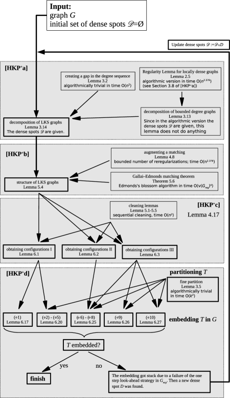
Figure 8.1: A version of [HKP⁺a, Figure LABEL:p0.fig:proofstructure] showing the iterative algorithm for finding a copy of $T$ in $G$.

The interesting question is if we can provide a fast algorithm which finds a copy of a given tree $T\in\mathbf{trees}({k})$ in any given graph $G\in\mathbf{LKS}({n},{k},{\alpha})$. We will sketch below that our proof gives such an algorithm, with running time $O(n^{6})$; here the hidden constant in the $O(\cdot)$-notation depends on $\alpha$ but not on $k$. A picture accompanying the discussion is given in Figure 8.1.

It can be verified that each of the steps of our proof — except the extraction of dense spots in [HKP⁺a]— can be turned into a polynomial time algorithm. We return to the extraction of dense spots later, after discussing the other parts of the proof.

• In [HKP⁺a, Section LABEL:p0.sssec:DecomposeAlgorithmically] we discussed the algorithmic aspects of obtaining a sparse decomposition of $G$, which is the main result ([HKP⁺a, Lemma LABEL:p0.lem:LKSsparseClass]) of [HKP⁺a]. This part contains the bottleneck step of the extraction of dense spots (in [HKP⁺a, Lemma LABEL:p0.lem:decompositionIntoBlackandExpanding]).

• In [HKP⁺b] we find a “rough structure” in $G$. Here, we need to find a matching in $\mathbf{G}_{\mathrm{reg}}$ that is maximal in a certain way, and we also need to “augment a regularized matching”. The former step can be done using Edmonds’s blossom algorithm, and the latter by applying the algorithmic version of the regularity lemma [ADL⁺94]. (We used [ADL⁺94] already in obtaining a sparse decomposition in [HKP⁺a].)

• In [HKP⁺c] we apply “cleaning lemmas” to refine the rough structure. The cleaning lemmas proceed by sequentially removing of “bad” vertices, and the respective badness conditions can be efficiently tested. The cleaning procedure are then put together in [HKP⁺c, Lemma LABEL:p2.lem:ConfWhenCXAXB–LABEL:p2.lem:ConfWhenMatching]. These lemmas are easily turned into algorithms.

• In the present paper we embed $T$ in $G$ using one of the configurations obtained in [HKP⁺c]. The basic ingredients of the embedding are the following:

  • Embedding in huge degree vertices (in $\mathbf{(\diamond 2)}$–$\mathbf{(\diamond 5)}$)
    The two main technical lemmas used are Lemmas 6.18 and 6.19. In these lemmas, in each step of the embedding we find a vertex having a substantial degree into one of the specified sets. So, the non-trivial assertions of these lemmas is that these good vertices exist. On the other hand, testing whether a given vertex is good can be done algorithmically (in time $O(n^{2}$)).

  • Embedding into regular pairs
    The exact setting is described in Lemmas 6.7–6.9, but the way we proceed with embedding of small trees is standard. That is, when we extend an embedding of a small tree or forest in a regular pair $(X,Y)$, we find a vertex of one cluster that has a substantial degree to the unused part of the partner cluster (the existence of which is guaranteed by the regularity). This can be implemented in time $O(|X||Y|)$.

  • Embedding into $G_{\mathrm{exp}}$
    The embedding procedure for embedding into $G_{\mathrm{exp}}$ was informally described in [HKP⁺a, Section LABEL:p0.sssec:whyGexp] and the actual setting we use is given in Lemma 6.5. The procedure is algorithmic. Indeed, when, in the proof of Lemma 6.5, we extend a partial embedding of a forest, it is enough to avoid the set called $\mathrm{shadow}_{H_{\mathrm{L}\ref{lem:embed:greyFOREST}}}(U_{\mathrm{L}\ref{lem:embed:greyFOREST}},\zeta_{\mathrm{L}\ref{lem:embed:greyFOREST}}k/2)$. This set can be easily determined algorithmically.

  • Embedding using $\mathbb{E}$
    Let us recall the elementary embedding procedure for $\mathbb{E}$ as described in Lemma 6.4. We have a small rooted tree $(T,r)$ (or several small rooted trees), a forbidden set $U$, and a set $U^{*}\subseteq\mathbb{E}$. It is our task to embed $T$, avoiding the set $U$, so that $r$ is placed in $U^{*}$. For the proof of Lemma 6.4 we only use the “avoiding” feature of the avoiding set given by Definition 4.5. That is, for each $y\in U^{*}$ we test whether there is a dense spot $D\in\mathcal{D}$ with $|U\cap V(D)|\leqslant\gamma^{2}k$ such that $y$ sends a substantial degree to $D$, or whether $y$ belongs to the bad set $Y_{\mathrm{ProofL}\ref{lem:embed:avoidingFOREST}}$. This test can be made algorithmic by simply ranging over the at most $O(n/k)$ dense spots in $\mathcal{D}$.

  The two randomized steps — random splitting in [HKP⁺c, Section LABEL:p2.ssec:RandomSplittins], and the use of the stochastic process $\mathsf{Duplicate}$ in Section 6 — can be also efficiently derandomized using a standard technique for derandomizing the Chernoff bound.

Let us now sketch how to deal with extracting dense spots. The idea is as follows. Initially, we pretend that $G_{\mathrm{exp}}$ consists of the entire bounded-degree part $G-\mathbb{H}$ (cleaned for minimum degree $\rho k$ as in [HKP⁺a, (LABEL:p0.eq:almostalldashed)]). With such a supposed sparse decomposition $\nabla_{1}$ we go through [HKP⁺b, Lemma LABEL:p1.prop:LKSstruct] and [HKP⁺c, Lemma LABEL:p2.outerlemma] to obtain a configuration. We now start embedding $T$ as in Section 6. (Note that at this moment $G_{\mathrm{reg}}$ and $\mathbb{E}$ are absent, and so, the only embedding techniques are those involving $\mathbb{H}$ and $G_{\mathrm{exp}}$.) Now, either we embed $T$, or we fail. The only possible reason for failure is that we were unable to perform the one-step look-ahead strategy described in [HKP⁺a, Section LABEL:p0.sssec:whyGexp], because $G_{\mathrm{exp}}$ was not really nowhere-dense. (In order to understand fully that this is indeed the only possible reason, the reader is advised to read the explanatory, two-pages-long Section LABEL:p0.sssec:whyGexp of [HKP⁺a].) But then we actually localized a dense spot $D_{1}$. We get an updated supposed sparse decomposition $\nabla_{2}$ in which $D_{1}$ is removed from $G_{\mathrm{exp}}$ and added to $\mathcal{D}$ (and $G_{\mathrm{reg}}$ and/or $\mathbb{E}$ are modified accordingly). We keep iterating. Since in each step we extract at least $O(k^{2})$ edges we iterate the above at most $e(G)/\Theta(k^{2})=O(\frac{n}{k})$ times. We certainly succeed eventually, since after $\Theta(\frac{n}{k})$ iterations we get an honest sparse decomposition (i.e., a decomposition that would be a valid outcome of [HKP⁺a, Lemma LABEL:p0.lem:LKSsparseClass], with $G_{\mathrm{exp}}$ nowhere-dense).

It seems that this iterative method is generally applicable for problems which employ a sparse decomposition.

9 Acknowledgments

The work on this project lasted from the beginning of 2008 until 2014 and we are very grateful to the following institutions and funding bodies for their support.

During the work on this paper Hladký was also affiliated with Zentrum Mathematik, TU Munich and Department of Computer Science, University of Warwick. Hladký was funded by a BAYHOST fellowship, a DAAD fellowship, Charles University grant GAUK 202-10/258009, EPSRC award EP/D063191/1, and by an EPSRC Postdoctoral Fellowship while working on the project.

Komlós and Szemerédi acknowledge the support of NSF grant DMS-0902241.

Piguet was also affiliated with the Institute of Theoretical Computer Science, Charles University in Prague, Zentrum Mathematik, TU Munich, the Department of Computer Science and DIMAP, University of Warwick, and the School of Mathematics, University of Birmingham. The work leading to this invention was supported by the European Regional Development Fund (ERDF), project “NTIS — New Technologies for Information Society”, European Centre of Excellence, CZ.1.05/1.1.00/02.0090. The research leading to these results has received funding from the European Union Seventh Framework Programme (FP7/2007-2013) under grant agreement no. PIEF-GA-2009-253925. Piguet acknowledges the support of the Marie Curie fellowship FIST, DFG grant TA 309/2-1, a DAAD fellowship, Czech Ministry of Education project 1M0545, EPSRC award EP/D063191/1, and the support of the EPSRC Additional Sponsorship, with a grant reference of EP/J501414/1 which facilitated her to travel with her young child and so she could continue to collaborate closely with her coauthors on this project. This grant was also used to host Stein in Birmingham.

Stein was affiliated with the Institute of Mathematics and Statistics, University of São Paulo, and the Center for Mathematical Modeling, University of Chile. She was supported by a FAPESP fellowship, and by FAPESP travel grant PQ-EX 2008/50338-0, also CMM-Basal, FONDECYT grants 11090141 and 1140766. She also received funding by EPSRC Additional Sponsorship EP/J501414/1.

We enjoyed the hospitality of the School of Mathematics of University of Birmingham, Center for Mathematical Modeling, University of Chile, Alfréd Rényi Institute of Mathematics of the Hungarian Academy of Sciences and Charles University, Prague, during our long term visits.

The yet unpublished work of Ajtai, Komlós, Simonovits, and Szemerédi on the Erdős–Sós Conjecture was the starting point for our project, and our solution crucially relies on the methods developed for the Erdős-Sós Conjecture. Hladký, Piguet, and Stein are very grateful to the former group for explaining them those techniques.

A doctoral thesis entitled Structural graph theory submitted by Hladký in September 2012 under the supervision of Daniel Král at Charles University in Prague is based on the series of the papers [HKP⁺a, HKP⁺b, HKP⁺c] and the present paper. The texts of the two works overlap greatly. We are grateful to PhD committee members Peter Keevash and Michael Krivelevich. Their valuable comments are reflected in the series.

We thank the referees for their very helpful remarks.

The contents of this publication reflects only the authors’ views and not necessarily the views of the European Commission of the European Union.

mathsymbolsSymbol index generalGeneral index

References

- [ADL+94] N. Alon, R. Duke, H. Lefmann, V. Rödl, and R. Yuster. The algorithmic aspects of the regularity lemma. J. Algorithms, 16:80–109, 1994.
- [AKS95] M. Ajtai, J. Komlós, and E. Szemerédi. On a conjecture of Loebl. In Graph theory, combinatorics, and algorithms, Vol. 1, 2 (Kalamazoo, MI, 1992), Wiley-Intersci. Publ., pages 1135–1146. Wiley, New York, 1995.
- [EFLS95] P. Erdős, Z. Füredi, M. Loebl, and V. T. Sós. Discrepancy of trees. Studia Sci. Math. Hungar., 30(1-2):47–57, 1995.
- [HKP+a] J. Hladký, J. Komlós, D. Piguet, M. Simonovits, M. Stein, and E. Szemerédi. The approximate Loebl–Komlós–Sós Conjecture I: The sparse decomposition. Manuscript (arXiv:1408.3858).
- [HKP+b] J. Hladký, J. Komlós, D. Piguet, M. Simonovits, M. Stein, and E. Szemerédi. The approximate Loebl–Komlós–Sós Conjecture II: The rough structure of LKS graphs. Manuscript (arXiv:1408.3871).
- [HKP+c] J. Hladký, J. Komlós, D. Piguet, M. Simonovits, M. Stein, and E. Szemerédi. The approximate Loebl–Komlós–Sós Conjecture III: The finer structure of LKS graphs. Manuscript (arXiv:1408.3866).
- [HP16] J. Hladký and D. Piguet. Loebl-Komlós-Sós Conjecture: dense case. J. Combin. Theory Ser. B, 116:123–190, 2016.
- [PS12] D. Piguet and M. J. Stein. An approximate version of the Loebl-Komlós-Sós conjecture. J. Combin. Theory Ser. B, 102(1):102–125, 2012.
- [Zha11] Y. Zhao. Proof of the conjecture for large . Electron. J. Combin., 18(1):Paper 27, 61, 2011.