Animated phase portraits of nonlinear and chaotic dynamical systems
Jean-Marc Ginoux11 Laboratoire Protee, I.U.T. de Toulon,
Senior lecturer in Applied Mathematics,
Doctor in Mathematics, Doctor in History of Sciences,
Université du Sud, BP 20132, F-83957 La Garde cedex, France
ginoux@univ-tln.fr, http://ginoux.univ-tln.fr
1991 Mathematics Subject Classification:
1. Introduction
The aim of this section is to present programs allowing to highlight the slow-fast evolution of the solutions of nonlinear and chaotic dynamical systems such as: Van der Pol, Chua and Lorenz models. These programs provide animated phase portraits in dimension two and three, i.e. “integration step by step” which are useful tools enabling to understand the dynamic of such systems.
2. Van der Pol model
The oscillator of B. Van der Pol [6] is a second-order system with non-linear frictions which can be written:
The particular form of the friction which can be carried out by an electric circuit causes a decrease of the amplitude of the great oscillations and an increase of the small. This equation constitutes the “paradigm of relaxation-oscillations”. According to D’Alembert transformation [1] any single order differential equation may be transformed into a system of simultaneous first-order equations and conversely. Let’s consider that: and let’s pose: and . Thus, we have:
When becomes very large, becomes a “fast” variable
and a “slow” variable. In order to analyze the limit , we introduce a small parameter and a “slow time” . Thus,
the system can be written:
(1)
with a small positive real parameter . System (1) which has been extensively studied since nearly one century is called a slow-fast dynamical system or a singularly perturbed dynamical system111See for example Ginoux [3].. Although, it has been established that system (1) can not be integrated by quadratures (closed-form) it is well-known that it admits a solution of limit-cycle type. The program presented here enables to emphasize the slow-fast evolutions of the solution on this limit-cycle.
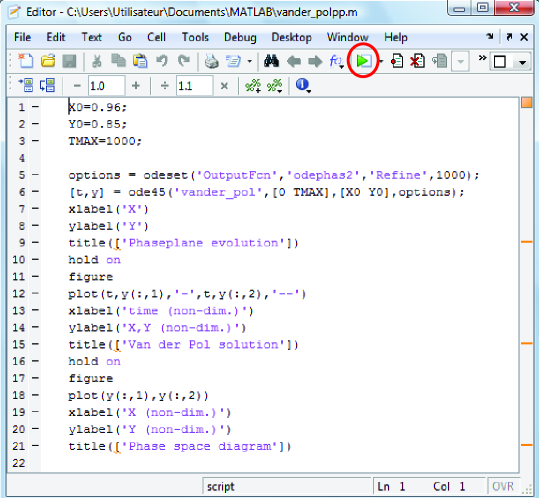
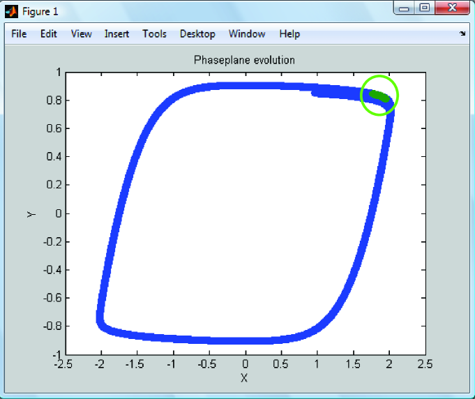
First, copy the files named “vanderpol” and “vanderpolpp” into the “current folder” of MatLab. Then, open the m-file called “vanderpolpp” (see Fig. 1) and press the green button (red circle on the Fig. 1) to provide an animated plot 2D. On the Fig. 2 the solution materialized by a green point (green circle on the Fig. 2) which evolves on the limit cycle, i.e., slowly on the nearly vertical parts and fast on the nearly horizontal parts.
Figure 1. Program for 2D animated phase portrait
All the main functions222See the textbook of Prof. Rudra Pratap [5] are described in Tab. 1:
Property
Description
OutputFcn
A function for the solver to call after every successful integration step.
odephas2
2D phase plane
Refine
Increases the number of output points by a factor of Refine.
Table 1. Description of the main functions
The program provides the animated phase portrait corresponding to the solution of system (1) and the time series.
Figure 2. Animated phase portrait in 2D
3. Chua’s model
The L.O. Chua’s circuit [2] is a relaxation oscillator with a cubic non-linear characteristic elaborated from a circuit comprising a harmonic oscillator of which operation is based on a field-effect transistor, coupled to a relaxation-oscillator composed of a tunnel diode. The modeling of the circuit uses a capacity which will
prevent from abrupt voltage drops and will make it possible to describe the fast motion of this oscillator by the following equations which also constitute a slow-fast dynamical system or a singularly perturbed dynamical system.
(2)
with and are real parameters , . The system (2) which can not be integrated by quadratures (closed-form) exhibits a solution evolving on “chaotic attractor” in the shape of a “double-scroll”. The program presented here enables to emphasize the slow-fast evolutions of the solution on the “chaotic attractor”.
First, copy the files named “chua” and “chua1” into the “current folder” of MatLab. Then, open the m-file called “chua1” and press the green button to provide an animated plot 3D. The solution materialized by a green point evolves on the attractor according to slow and fast motion. The function “odephas2” is simply replaced by “odephas3”.
4. Lorenz model
The purpose of the model established by Edward Lorenz [4] was in the beginning to analyze the unpredictable behavior of weather. After having developed non-linear partial derivative equations starting from the thermal equation and Navier-Stokes equations, Lorenz truncated them to retain only three modes. The most widespread form of the Lorenz model is as follows:
(3)
with , , and are real parameters: , , .
Although, this system is notsingularly perturbed since it does not contain any small multiplicative parameter, it is a slow-fast dynamical system. Its solution exhibits a solution evolving on “chaotic attractor” in the shape of a “butterfly”. The program presented here enables to emphasize the slow-fast evolutions of the solution on the “chaotic attractor”.
Table 2. List of program for animated phase portraits.
References
[1]J. D’Alembert, Suite des recherches sur le calcul intégral, quatrième partie : Méthodes pour intégrer quelques équations différentielles, Hist. Acad. Berlin, tome IV (1748) 275-291.
[2]L.O. Chua, M. Komuro & T. Matsumoto, “The double scroll family,” IEEE Trans. on Circuits and Systems, 33(11) (1986) 1072-1097.
[3]J.M. Ginoux, Differential geometry applied to dynamical systems, World Scientific
Series on Nonlinear Science, Series A 66 (World Scientific, Singapore), 2009.
[4]E. N. Lorenz, “Deterministic non-periodic flows,” Journal of Atmospheric
Sciences, 20 (1963) 130-141.
[5]R. Pratap, Getting Started with MATLAB: A Quick Introduction for Scientists and Engineers, Oxford University Press, USA (November 16, 2009).
[6]B. Van der Pol, “On ’Relaxation-Oscillations’,” Philosophical Magazine, 7(2) (1926) 978-992.