Slow Manifold of a Neuronal Bursting Model

Abstract

Comparing neuronal bursting models (NBM) with slow-fast autonomous dynamical systems (S-FADS), it appears that the specific features of a (NBM) do not allow a determination of the analytical slow manifold equation with the singular approximation method. So, a new approach based on Differential Geometry, generally used for (S-FADS), is proposed. Adapted to (NBM), this new method provides three equivalent manners of determination of the analytical slow manifold equation. Application is made for the three-variables model of neuronal bursting elaborated by Hindmarsh and Rose which is one of the most used mathematical representation of the widespread phenomenon of oscillatory burst discharges that occur in real neuronal cells.

1 Slow-fast autonomous dynamical systems, neuronal bursting models

1.1 Dynamical systems

In the following we consider a system of differential equations defined in a compact E included in $\mathbb{R}$:

$$\frac{d{\vec{X}}}{dt}=\vec{\Im}\left(\vec{X}\right)$$ (1)

with

$$\vec{X}=\left[{x_{1},x_{2},...,x_{n}}\right]^{t}\in E\subset\mathbb{R}^{n}$$

and

$$\vec{\Im}\left(\vec{X}\right)=\left[{f_{1}\left(\vec{X}\right),f_{2}\left(\vec{X}\right),...,f_{n}\left(\vec{X}\right)}\right]^{t}\in E\subset\mathbb{R}^{n}$$

The vector $\vec{\Im}\left(\vec{X}\right)$ defines a velocity vector field in E whose components $f_{i}$ which are supposed to be continuous and infinitely differentiable with respect to all $x_{i}$ and $t$, i.e., are $C^{\infty}$ functions in E and with values included in $\mathbb{R}$, satisfy the assumptions of the Cauchy-Lipschitz theorem. For more details, see for example [2]. A solution of this system is an integral curve $\vec{X}\left(t\right)$ tangent to $\vec{\Im}$ whose values define the states of the dynamical system described by the Eq. (1). Since none of the components $f_{i}$ of the velocity vector field depends here explicitly on time, the system is said to be autonomous.

1.2 Slow-fast autonomous dynamical system (S-FADS)

A (S-FADS) is a dynamical system defined under the same conditions as previously but comprising a small multiplicative parameter $\varepsilon$ in one or several components of its velocity vector field:

$$\frac{d{\vec{X}}}{dt}=\vec{\Im}_{\varepsilon}\left(\vec{X}\right)$$ (2)

with

$$\vec{\Im}_{\varepsilon}\left(\vec{X}\right)=\left[{\frac{1}{\varepsilon}f_{1}\left(\vec{X}\right),f_{2}\left(\vec{X}\right),...,f_{n}\left(\vec{X}\right)}\right]^{t}\in E\subset\mathbb{R}^{n}$$

$$0<\varepsilon\ll 1$$

The functional jacobian of a (S-FADS) defined by (2) has an eigenvalue called “fast”, i.e., great on a large domain of the phase space. Thus, a “fast” eigenvalue is expressed like a polynomial of valuation $-1$ in $\varepsilon$ and the eigenmode which is associated with this “fast” eigenvalue is said:

- “evanescent” if it is negative,

- “dominant” if it is positive.

The other eigenvalues called “slow” are expressed like a polynomial of valuation $0$ in $\varepsilon$.

1.3 Neuronal bursting models (NBM)

A (NBM) is a dynamical system defined under the same conditions as previously but comprising a large multiplicative parameter $\varepsilon^{-1}$ in one component of its velocity vector field:

$$\frac{d{\vec{X}}}{dt}=\vec{\Im}_{\varepsilon}\left(\vec{X}\right)$$ (3)

with

$$\vec{\Im}_{\varepsilon}\left(\vec{X}\right)=\left[{f_{1}\left(\vec{X}\right),f_{2}\left(\vec{X}\right),...,\varepsilon f_{n}\left(\vec{X}\right)}\right]^{t}\in E\subset\mathbb{R}^{n}$$

$$0<\varepsilon\ll 1$$

The presence of the multiplicative parameter $\varepsilon^{-1}$ in one of the components of the velocity vector field makes it possible to consider the system (3) as a kind of slow-fast autonomous dynamical system (S-FADS). So, it possesses a slow manifold, the equation of which may be determined. But, paradoxically, this model is not slow-fast in the sense defined previously. A comparison between three-dimensional (S-FADS) and (NBM) presented in Table 1 emphasizes their differences. The dot $(\cdot)$ represents the derivative with respect to time and $\varepsilon\ll 1$.

Table 1: Comparison between (S-FADS) and (NBM)

(S-FADS) vs (NBM)
$\hskip 7.22743pt\dfrac{d{\vec{X}}}{dt}\left({{\begin{array}[]{*{20}c}\dot{x}\hfill\\ \dot{y}\hfill\\ \dot{z}\hfill\\ \end{array}}}\right)=\vec{\Im_{\varepsilon}}\left({{\begin{array}[]{*{20}c}{\dfrac{1}{\varepsilon}f\left({x,y,z}\right)\vspace{4pt}}\\ {\mbox{ }g\left({x,y,z}\right)\vspace{4pt}}\\ {h\left({x,y,z}\right)}\\ \end{array}}}\right)\mbox{ }$	$\hskip 7.22743pt\dfrac{d{\vec{X}}}{dt}\left({{\begin{array}[]{*{20}c}\dot{x}\hfill\\ \dot{y}\hfill\\ \dot{z}\hfill\\ \end{array}}}\right)=\vec{\Im_{\varepsilon}}\left({{\begin{array}[]{*{20}c}{\mbox{ }f\left({x,y,z}\right)\vspace{4pt}}\\ {\mbox{ }g\left({x,y,z}\right)\vspace{4pt}}\\ {\varepsilon h\left({x,y,z}\right)}\\ \end{array}}}\right)\mbox{ }$
$\hskip 7.22743pt\dfrac{d{\vec{X}}}{dt}\left({{\begin{array}[]{*{20}c}\dot{x}\hfill\\ \dot{y}\hfill\\ \dot{z}\hfill\\ \end{array}}}\right)=\vec{\Im_{\varepsilon}}\left({{\begin{array}[]{*{20}c}{\mbox{ }fast\vspace{4pt}}\\ {\mbox{ }slow\vspace{4pt}}\\ {slow}\\ \end{array}}}\right)\mbox{ }$	$\hskip 7.22743pt\dfrac{d{\vec{X}}}{dt}\left({{\begin{array}[]{*{20}c}\dot{x}\hfill\\ \dot{y}\hfill\\ \dot{z}\hfill\\ \end{array}}}\right)=\vec{\Im_{\varepsilon}}\left({{\begin{array}[]{*{20}c}{\mbox{ }fast\vspace{4pt}}\\ {\mbox{ }fast\vspace{4pt}}\\ {slow}\\ \end{array}}}\right)\mbox{ }$

2 Analytical slow manifold equation

There are many methods of determination of the analytical equation of the slow manifold. The classical one based on the singular perturbations theory [1] is the so-called singular approximation method. But, in the specific case of a (NBM), one of the hypothesis of the Tihonov’s theorem is not checked since the fast dynamics of the singular approximation has a periodic solution. Thus, another approach developed in [4] which consist in using Differential Geometry formalism may be used.

2.1 Singular approximation method

The singular approximation of the fast dynamics constitutes a quite good approach since the third component of the velocity is very weak and so, $z$ is nearly constant along the periodic solution. In dimension three the system (3) can be written as a system of differential equations defined in a compact E included in $\mathbb{R}$:

$$\hskip 7.22743pt\frac{d{\vec{X}}}{dt}=\left({{\begin{array}[]{*{20}c}{\frac{d{x}}{dt}\vspace{4pt}}\\ {\frac{d{y}}{dt}\vspace{4pt}}\\ {\frac{d{z}}{dt}}\\ \end{array}}}\right)=\vec{\Im}_{\varepsilon}\left({{\begin{array}[]{*{20}c}{\mbox{ }f\left({x,y,z}\right)\vspace{4pt}}\\ {\mbox{ }g\left({x,y,z}\right)\vspace{4pt}}\\ {\varepsilon h\left({x,y,z}\right)}\\ \end{array}}}\right)$$

On the one hand, since the system (3) can be considered as a (S-FADS), the slow dynamics of the singular approximation is given by:

$$\hskip 28.90755pt\left\{{{\begin{array}[]{*{20}c}{f\left({x,y,z}\right)=0\hfill}\\ {g\left({x,y,z}\right)=0\hfill}\\ \end{array}}}\right.$$ (4)

The resolution of this reduced system composed of the two first equations of the right hand side of (3) provides a one-dimensional singular manifold, called singular curve. This curve doesn’t play any role in the construction of the periodic solution. But we will see that there exists all the more a slow dynamics. On the other hands, it presents a fast dynamics which can be given while posing the following change:

$$\tau=\varepsilon t\mbox{ }\Leftrightarrow\mbox{ }\frac{d}{dt}=\varepsilon\frac{d}{d{\tau}}$$

The system (3) may be re-written as:

$$\frac{d{\vec{X}}}{d{\tau}}=\left({{\begin{array}[]{*{20}c}{\frac{d{x}}{d{\tau}}\vspace{4pt}}\\ {\frac{d{y}}{d{\tau}}\vspace{4pt}}\\ {\frac{d{z}}{d{\tau}}}\\ \end{array}}}\right)=\vec{\Im_{\varepsilon}}\left({{\begin{array}[]{*{20}c}{\varepsilon^{-1}f\left({x,y,z}\right)\vspace{4pt}}\\ {\varepsilon^{-1}g\left({x,y,z}\right)\vspace{4pt}}\\ {\mbox{ }h\left({x,y,z}\right)}\\ \end{array}}}\right)$$ (5)

So, the fast dynamics of the singular approximation is provided by the study of the reduced system composed of the two first equations of the right hand side of (5).

$$\left.{\frac{d{\vec{X}}}{d{\tau}}}\right|_{fast}=\left({{\begin{array}[]{*{20}c}{\frac{d{x}}{d{\tau}}\vspace{4pt}}\\ {\frac{d{y}}{d{\tau}}}\\ \end{array}}}\right)=\vec{\Im_{\varepsilon}}\left({{\begin{array}[]{*{20}c}{\varepsilon^{-1}f\left({x,y,z^{\ast}}\right)\vspace{4pt}}\\ {\varepsilon^{-1}g\left({x,y,z^{\ast}}\right)}\\ \end{array}}}\right)$$ (6)

Each point of the singular curve is a singular point of the singular approximation of the fast dynamics. For the $z$ value for which there is a periodic solution, the singular approximation exhibits an unstable focus, attractive with respect to the slow eigendirection.

2.2 Differential Geometry formalism

Now let us consider a three-dimensional system defined by (3) and let’s define the instantaneous acceleration vector of the trajectory curve $\vec{X}\left(t\right)$. Since the functions $f_{i}$ are supposed to be $C^{\infty}$ functions in a compact E included in $\mathbb{R}$, it is possible to calculate the total derivative of the vector field $\vec{\Im_{\varepsilon}}$. As the instantaneous vector function $\vec{V}\left(t\right)$ of the scalar variable $t$ represents the velocity vector of the mobile M at the instant $t$, the total derivative of $\vec{V}\left(t\right)$ is the vector function $\vec{\gamma}\left(t\right)$ of the scalar variable $t$ which represents the instantaneous acceleration vector of the mobile M at the instant $t$. It is noted:

$$\vec{\gamma}\left(t\right)\mbox{ }=\mbox{ }\frac{d{\vec{V}}\left(t\right)}{dt}$$ (7)

Even if neuronal bursting models are not exactly slow-fast autonomous dynamical systems, the new approach of determining the slow manifold equation developed in [4] may still be applied. This method is using Differential Geometry properties such as curvature and torsion of the trajectory curve $\vec{X}\left(t\right)$, integral of dynamical systems to provide their slow manifold equation.

Proposition 2.1

The location of the points where the local torsion of the trajectory curves integral of a dynamical system defined by (3) vanishes, provides the analytical equation of the slow manifold associated with this system.

$$\frac{1}{\Im}=-\frac{\dot{\vec{\gamma}}\cdot\left({\vec{\gamma}\times\vec{V}}\right)}{\left\|{\vec{\gamma}\times\vec{V}}\right\|^{2}}=0\mbox{ }\Leftrightarrow\mbox{ }\dot{\vec{\gamma}}\cdot\left({\vec{\gamma}\times\vec{V}}\right)=0$$ (8)

Thus, this equation represents the slow manifold of a neuronal bursting model defined by (3).

The particular features of neuronal bursting models (3) will lead to a simplification of this Proposition 1. Due to the presence of the small multiplicative parameter $\varepsilon$ in the third components of its velocity vector field, instantaneous velocity vector $\vec{V}\left(t\right)$ and instantaneous acceleration vector $\vec{\gamma}\left(t\right)$ of the model (3) may be written:

$$\hskip 28.90755pt\vec{V}\left({{\begin{array}[]{*{20}c}\dot{x}\hfill\\ \dot{y}\hfill\\ \dot{z}\hfill\\ \end{array}}}\right)=\vec{\Im}_{\varepsilon}\left({{\begin{array}[]{*{20}c}{O\left({\varepsilon^{0}}\right)\vspace{4pt}}\\ {O\left({\varepsilon^{0}}\right)\vspace{4pt}}\\ {O\left({\varepsilon^{1}}\right)\vspace{4pt}}\\ \end{array}}}\right)$$ (9)

and

$$\hskip 21.68121pt\vec{\gamma}\left({{\begin{array}[]{*{20}c}\ddot{x}\hfill\\ \ddot{y}\hfill\\ \ddot{z}\hfill\\ \end{array}}}\right)=\frac{d{\vec{\Im}_{\varepsilon}}}{dt}\left({{\begin{array}[]{*{20}c}{O\left({\varepsilon^{1}}\right)\vspace{4pt}}\\ {O\left({\varepsilon^{1}}\right)\vspace{4pt}}\\ {O\left({\varepsilon^{2}}\right)\vspace{4pt}}\\ \end{array}}}\right)$$ (10)

where ${O\left({\varepsilon^{n}}\right)}$ is a polynomial of $n$ degree in $\varepsilon$

Then, it is possible to express the vector product $\vec{V}\times\vec{\gamma}$ as:

$$\hskip 28.90755pt\vec{V}\times\vec{\gamma}=\left({{\begin{array}[]{*{20}c}{\dot{y}\ddot{z}-\ddot{y}\dot{z}\hfill}\\ {\ddot{x}\dot{z}-\dot{x}\ddot{z}\hfill}\\ {\dot{x}\ddot{y}-\ddot{x}\dot{y}\hfill}\\ \end{array}}}\right)$$ (11)

Taking into account what precedes (9, 10), it follows that:

$$\hskip 28.90755pt\vec{V}\times\vec{\gamma}=\left({{\begin{array}[]{*{20}c}{O\left({\varepsilon^{2}}\right)\vspace{4pt}}\\ {O\left({\varepsilon^{2}}\right)\vspace{4pt}}\\ {O\left({\varepsilon^{1}}\right)\vspace{4pt}}\\ \end{array}}}\right)$$ (12)

So, it is obvious that since $\varepsilon$ is a small parameter, this vector product may be written:

$$\hskip 28.90755pt\vec{V}\times\vec{\gamma}\approx\left({{\begin{array}[]{*{20}c}0\\ 0\\ {O\left({\varepsilon^{1}}\right)}\\ \end{array}}}\right)$$ (13)

Then, it appears that if the third component of this vector product vanishes when both instantaneous velocity vector $\vec{V}\left(t\right)$ and instantaneous acceleration vector $\vec{\gamma}\left(t\right)$ are collinear. This result is particular to this kind of model which presents a small multiplicative parameter in one of the right-hand-side component of the velocity vector field and makes it possible to simplify the previous Proposition 1.

Proposition 2.2

The location of the points where the instantaneous velocity vector $\vec{V}\left(t\right)$ and instantaneous acceleration vector $\vec{\gamma}\left(t\right)$ of a neuronal bursting model defined by (3) are collinear provides the analytical equation of the slow manifold associated with this dynamical system.

$$\vec{V}\times\vec{\gamma}=\vec{0}\mbox{ }\Leftrightarrow\mbox{ }\dot{x}\ddot{y}-\ddot{x}\dot{y}=0$$ (14)

Another method of determining the slow manifold equation proposed in [14] consists in considering the so-called tangent linear system approximation. Then, a coplanarity condition between the instantaneous velocity vector $\vec{V}\left(t\right)$ and the slow eigenvectors of the tangent linear system gives the slow manifold equation.

$$\vec{V}.\left({\vec{Y_{\lambda_{2}}}\times\vec{Y_{\lambda_{3}}}}\right)=0$$ (15)

where $\vec{Y_{\lambda_{i}}}$ represent the slow eigenvectors of the tangent linear system. But, if these eigenvectors are complex the slow manifold plot may be interrupted. So, in order to avoid such inconvenience, this equation has been multiplied by two conjugate equations obtained by circular permutations.

$$\left[{\vec{V}\cdot\left({\vec{Y_{\lambda_{2}}}\times\vec{Y_{\lambda_{3}}}}\right)}\right]\cdot\left[{\vec{V}\cdot\left({\vec{Y_{\lambda_{1}}}\times\vec{Y_{\lambda_{2}}}}\right)}\right]\cdot\left[{\vec{V}\cdot\left({\vec{Y_{\lambda_{1}}}\times\vec{Y_{\lambda_{3}}}}\right)}\right]=0$$

It has been established in [4] that this real analytical slow manifold equation can be written:

$$\left({J^{2}\vec{V}}\right)\cdot\left({\vec{\gamma}\times\vec{V}}\right)=0$$ (16)

since the the tangent linear system approximation method implies to suppose that the functional jacobian matrix is stationary. That is to say

$$\frac{dJ}{dt}=0$$

and so,

$$\dot{\vec{\gamma}}=J\frac{d{\vec{V}}}{dt}+\frac{dJ}{dt}\vec{V}=J\vec{\gamma}+\frac{dJ}{dt}\vec{V}=J^{2}\vec{V}+\frac{dJ}{dt}\vec{V}\approx J^{2}\vec{V}$$

Proposition 2.3

The coplanarity condition (15) between the instantaneous velocity vector and the slow eigenvectors of the tangent linear system transformed into the real analytical equation (16) provides the slow manifold equation of a neuronal bursting model defined by (3).

3 Application to a neuronal bursting model

The transmission of nervous impulse is secured in the brain by action potentials. Their generation and their rhythmic behaviour are linked to the opening and closing of selected classes of ionic channels. The membrane potential of neurons can be modified by acting on a combination of different ionic mechanisms. Starting from the seminal works of Hodgkin-Huxley [7, 11] and FitzHugh-Nagumo [3, 12], the Hindmarsh-Rose [6, 13] model consists of three variables: $x$, the membrane potential, $y$, an intrinsic current and $z$, a slow adaptation current.

3.1 Hindmarsh-Rose model of bursting neurons

$$\hskip 28.90755pt\left\{{{\begin{array}[]{{ll}}{\frac{d{x}}{dt}=y-f\left(x\right)-z+I\hfill\vspace{4pt}}\\ {\frac{d{y}}{dt}=g\left(x\right)-y\hfill\vspace{4pt}}\\ {\frac{d{z}}{dt}=\varepsilon\left({h\left(x\right)-z}\right)\hfill}\\ \end{array}}}\right.$$ (17)

$I$ represents the applied current, $f\left(x\right)=ax^{3}-bx^{2}$ and $g\left(x\right)=c-dx^{2}$ are respectively cubic and quadratic functions which have been experimentally deduced [5]. $\varepsilon$ is the time scale of the slow adaptation current and $h\left(x\right)=x-x^{\ast}$ is the scale of the influence of the slow dynamics, which determines whether the neuron fires in a tonic or in a burst mode when it is exposed to a sustained current input and where $\left({x^{\ast},y^{\ast}}\right)$ are the co-ordinates of the leftmost equilibrium point of the model (1) without adaptation, i.e., $I=0$.
Parameters used for numerical simulations are:
$a=1$, $b=3$, $c=1$, $d=5$, $\varepsilon=0.005$, $s=4$, $x^{\ast}=\frac{-1-\sqrt{5}}{2}$ and $I=3.25$.

While using the method proposed in the section 2 it is possible to determine the analytical slow manifold equation of the Hindmarsh-Rose 84’model [6].

3.2 Slow manifold of the Hindmarsh-Rose 84’model

In Fig. 1 is presented the slow manifold of the Hindmarsh-Rose 84’model determined with the Proposition 1.

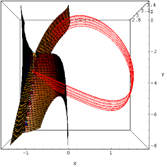
Figure 1: Slow manifold of the Hindmarsh-Rose 84’model with the Prop. 1.

The slow manifold provided with the use of the collinearity condition between both instantaneous velocity vector and instantaneous acceleration vector, i.e., while using the Proposition 2 is presented in Fig. 2.

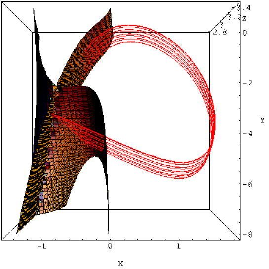
Figure 2: Slow manifold of the Hindmarsh-Rose 84’model with the Prop. 2.

Figure 3 presents the slow manifold of the Hindmarsh-Rose 84’model obtained with the tangent linear system approximation, i.e., with the use of Proposition 3.

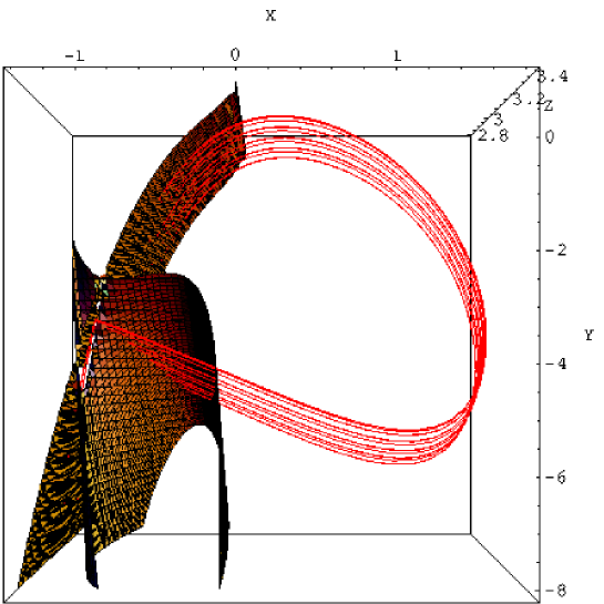
Figure 3: Slow manifold of the Hindmarsh-Rose 84’model with the Prop. 3.

4 Discussion

Since in the case of neuronal bursting model (NBM) bursting models one of the Tihonov’s hypothesis is not checked, the classical singular approximation method can not be used to determine the analytical slow manifold equation. In this work the application of the Differential Geometry formalism provides new alternative methods of determination of the slow manifold equation of a neuronal bursting model (NBM).

• the torsion method, i.e., the location of the points where the local torsion of the trajectory curve, integral of dynamical systems vanishes,

• the collinearity condition between the instantaneous velocity vector $\overrightarrow{V}$, the instantaneous acceleration vector $\overrightarrow{\gamma}$,

• the tangent linear system approximation, i.e., the coplanarity condition between the instantaneous velocity vector eigenvectors transformed into a real analytical equation.

The striking similarity of all figures due to the smallness of the parameter $\varepsilon$ highlights the equivalence between all the propositions. Moreover, even if the presence of this small parameter $\varepsilon$ in one of the right-hand-side component of the instantaneous velocity vector field of a (NBM) prevents from using the singular approximation method, it clarifies the Proposition 1 and transforms it into a collinearity condition in dimension three, i.e., Proposition 2. Comparing (S-FADS) and (NBM) in Table 1 it can be noted that in a (S-FADS) there is one fast component and two fast while in a (NBM) the situation is exactly reversed. Two fast components and one slow. So, considering (NBM) as a particular class of (S-FADS) we suggest to call (NBM) fast-slow instead of slow-fast in order to avoid any confusion. Further research should highlight other specific features of (NBM).

References

- [1] Andronov AA, Khaikin SE, & Vitt AA (1966) Theory of oscillators, Pergamon Press, Oxford
- [2] Coddington EA & Levinson N, (1955) Theory of Ordinary Differential Equations, Mac Graw Hill, New York
- [3] Fitzhugh R (1961) Biophys. J 1:445–466
- [4] Ginoux JM & Rossetto B (2006) Int. J. Bifurcations and Chaos, (in print)
- [5] Hindmarsh JL & Rose RM (1982) Nature 296:162–164
- [6] Hindmarsh JL & Rose RM (1984) Philos. Trans. Roy. Soc. London Ser. B 221:87–102
- [7] Hodgkin AL & Huxley AF (1952) J. Physiol. (Lond.) 116:473–96
- [8] Hodgkin AL & Huxley AF (1952) J. Physiol. (Lond.) 116: 449–72
- [9] Hodgkin AL & Huxley AF (1952) J. Physiol. (Lond.) 116: 497–506
- [10] Hodgkin AL & Huxley AF (1952) J. Physiol. (Lond.) 117: 500–44
- [11] Hodgkin AL, Huxley AF & Katz B (1952) B. Katz J. Physiol. (Lond.) 116: 424–48
- [12] Nagumo JS, Arimoto S & Yoshizawa S (1962) Proc. Inst. Radio Engineers 50:2061–2070
- [13] Rose RM & Hindmarsh JL (1985) Proc. R. Soc. Ser. B 225:161–193
- [14] Rossetto B, Lenzini T, Suchey G & Ramdani S (1998) Int. J. Bifurcation and Chaos, vol. 8 (11):2135-2145