Stable foliations and
semi-flow Morse homology

Abstract

In case of the heat flow on the free loop space of a closed Riemannian manifold non-triviality of Morse homology for semi-flows is established by constructing a natural isomorphism to singular homology of the loop space. The construction is also new in finite dimensions. The main idea is to build a Morse filtration using Conley pairs and their pre-images under the time-$T$-map of the heat flow. A crucial step is to contract each Conley pair onto its part in the unstable manifold. To achieve this we construct stable foliations for Conley pairs using the recently found backward $\lambda$-Lemma [31]. These foliations are of independent interest [23].

1 Main results

Consider a closed Riemannian manifold $(M,g)$. A smooth function $V\in C^{\infty}(S^{1}\times M)$, called potential, gives rise to the classical action functional

$${\mathcal{S}}_{V}(\gamma)=\int_{0}^{1}\left(\frac{1}{2}\left|\dot{\gamma}(t)\right|^{2}-V(t,\gamma(t))\right)dt$$

defined on the free loop space of $M$, that is the Hilbert manifold $\Lambda M=W^{1,2}(S^{1},M)$ which consists of all absolutely continuous maps $\gamma:S^{1}\to M$ whose first derivative is square integrable. Here and throughout we identify $S^{1}={\mathbb{R}}/{\mathbb{Z}}$ and think of maps defined on $S^{1}$ as $1$-periodic maps defined on ${\mathbb{R}}$. Let $\nabla$ be the Levi-Civita connection. The set ${\rm Crit}$ of critical points of ${\mathcal{S}}_{V}$ consists of the $1$-periodic solutions of the ODE

$$\nabla\kern-2.15277pt{}_{t}\dot{x}+\nabla V_{t}(x)=0$$ (1)

where $V_{t}(q):=V(t,q)$. For constant $V$ these are the closed geodesics. The negative $L^{2}$ gradient of ${\mathcal{S}}_{\mathcal{V}}$ is given by the left hand side of (1) and defined on a dense subset $W^{2,2}$ of $\Lambda M$. It generates a $C^{1}$ semi-flow

$$\varphi:(0,\infty)\times\Lambda M\to\Lambda M$$

which extends continuously to time zero, preserves sublevel sets, and is called the heat flow; see e.g. [5, 27, 28]. The semi-flow still exists for a class of abstract perturbations, introduced in [17], that take the form of smooth maps ${\mathcal{V}}:\Lambda M\to{\mathbb{R}}$ which satisfy certain axioms, say (V0)–(V3) in the notation of [28]. These perturbations allow to achieve Morse-Smale transversality generically; see [28]. They extend from the dense subset ${\mathcal{L}}M=C^{\infty}(S^{1},M)$ to $\Lambda M$ by (V0). Define $\varphi_{s}\gamma=u(s,\cdot)$ where $u:[0,\infty)\times S^{1}\to M$ solves the heat equation

$${\partial}_{s}u-\nabla\kern-2.15277pt{}_{t}{\partial}_{t}u-{\rm grad}{\mathcal{V}}(u)=0$$ (2)

with $u(0,\cdot)=\gamma$. If ${\mathcal{V}}(\gamma)=\int_{0}^{1}V_{t}(\gamma(t))dt$, then ${\rm grad}{\mathcal{V}}(u)=\nabla V_{t}(u)$; see [28].

1.1 Semi-flow Morse homology

From now on fix $V$ in the residual (hence dense) subset of $C^{\infty}(S^{1}\times M,{\mathbb{R}})$ for which ${\mathcal{S}}_{V}$ is a Morse function, that is all critical points are nondegenerate; see [26]. An oriented critical point $\langle x\rangle$ or $o_{x}$ is a critical point $x$ together with an orientation of the maximal vector subspace $E_{x}\subset T_{x}\Lambda M$ on which the Hessian of ${\mathcal{S}}_{\mathcal{V}}$ is negative definite. Recall that the dimension of $E_{x}$, denoted by ${\rm ind}_{V}(x)$, is finite and called the Morse index of $x$; see e.g. [26].

Chain groups

Fix a regular value $a$ of ${\mathcal{S}}_{V}$. The set ${\rm Crit}^{a}$ of critical points of the Morse function ${\mathcal{S}}_{V}$ defined on the sublevel set

$$\Lambda^{a}M=\{{\mathcal{S}}_{V}\leq a\}$$

is a finite set, see e.g. [26], hence the set ${\rm Crit}$ is countable. To avoid dependence of the Morse chain complex on the (traditionally taken and lamented) apriori choices of orientations a look at the construction of simplicial homology is useful; see e.g. [10, §5]. In this theory all simplices are taken oriented, because the algebraic boundary operator induces on (or transports to) the faces precisely the geometric boundary orientation which eventually leads to ${\partial}^{2}=0$. Then in a second step one factors out opposite orientations. In the context of Floer homology a similar approach was taken recently by Abbondandolo and Schwarz [2] who use oriented critical points as generators and then factor out opposite orientations. This requires a mechanism of orientation transport, but avoids having unnatural orientations built into the chain complex and therefore allows for a natural isomorphism to singular homology.

By definition the Morse chain group ${\rm CM}_{*}^{a}={\rm CM}_{*}^{a}(V)$ is the free abelian group generated by the (finite) set of oriented critical points $\langle x\rangle$, likewise denoted by $o_{x}$, below level $a$ and subject to the relations

$$o_{x}+\bar{o}_{x}=0,\qquad\forall x\in{\rm Crit}^{a},$$ (3)

where $\bar{o}_{x}$ is the orientation opposite to $o_{x}$. The Morse index provides a natural grading and ${\rm Crit}^{a}_{k}\subset{\rm Crit}^{a}$ denotes the set of critical points of Morse index $k$.

Boundary operator

Fix an element $v=v_{a}:\Lambda M\to{\mathbb{R}}$ of the set ${\mathcal{O}}^{a}_{reg}$ of regular perturbations defined in [28, §5], set

$${\mathcal{V}}(\gamma;V,v_{a})=v_{a}(\gamma)+\int_{0}^{1}V(t,\gamma(t))\,dt,$$ (4)

and note the following consequences. Firstly, on $\Lambda^{a}M$ the critical points of ${\mathcal{S}}_{V}$ and the perturbed action ${\mathcal{S}}_{\mathcal{V}}$, also called Morse-Smale function, given by

$${\mathcal{S}}_{\mathcal{V}}(\gamma)=\frac{1}{2}\int_{0}^{1}\left|\dot{\gamma}(t)\right|^{2}\,dt-{\mathcal{V}}(\gamma)$$ (5)

coincide by [28, §5 Prop. 8]. In abuse of notation we denote the perturbed action ${\mathcal{S}}_{\mathcal{V}}$ sometimes by ${\mathcal{S}}_{V+v_{a}}$. In fact, both functionals coincide on a neighborhood $U=U(V)$ in $\Lambda M$ of the set ${\rm Crit}$ of all critical points. Therefore the subspaces $E_{x}$ do not change under such perturbations. Secondly, the perturbed action ${\mathcal{S}}_{\mathcal{V}}$ is Morse Smale below level $a$ in the functional analytic sense of [28, §1].

By [28, §6 Thm. 18] the unstable manifold $W^{u}(x)=W^{u}(x;{\mathcal{V}})$ of any critical point $x$ is a contractible, thus orientable, smooth submanifold of $\Lambda M$ whose dimension is given by the Morse index $k={\rm ind}_{V}(x)$. On the other hand, for ${\varepsilon}={\varepsilon}(a)>0$ small the stable or ascending disk

$$W^{s}_{\varepsilon}(y)=W^{s}_{\varepsilon}(y;{\mathcal{V}}):=W^{s}(y;{\mathcal{V}})\cap\{{\mathcal{S}}_{\mathcal{V}}<{\mathcal{S}}_{\mathcal{V}}(y)+{\varepsilon}\}$$ (6)

of any $y\in{\rm Crit}^{a}$ is a $C^{1}$ Hilbert submanifold of $\Lambda M$ of finite codimension $\ell={\rm ind}_{V}(y)$. Since $T_{y}W^{u}(y)$ is the orthogonal complement of the tangent space at $y$ to the ascending disk $W^{s}_{\varepsilon}(y)$, an orientation of the unstable manifold determines a co-orientation of the (contractible) ascending disk and vice versa.

The functional analytic characterization of the Morse-Smale condition below level $a$ used in the definition of ${\mathcal{O}}^{a}_{reg}$ translates into the form common in dynamical systems, namely that all intersections

$$M_{xy}^{\varepsilon}:=W^{u}(x)\pitchfork{\rm W}^{s}_{\varepsilon}(y),\qquad\forall x,y\in{\rm Crit}^{a},$$ (7)

are cut out transversely from $\Lambda M$. Consequently these intersections are $C^{1}$ manifolds of dimension equal to the Morse index difference $k-\ell$. They are naturally oriented given an orientation of $W^{u}(x)$ and a co-orientation of $W^{s}_{\varepsilon}(y)$. More precisely, condition (7) implies that there is the pointwise splitting

$$T_{\gamma}W^{u}(x)\cong T_{\gamma}M_{xy}^{\varepsilon}\oplus\left(T_{\gamma}W^{s}_{\varepsilon}(y)\right)^{\perp},\qquad\gamma\in M_{xy}^{\varepsilon},$$ (8)

into two orthogonal subspaces. Furthermore, for generic $\delta\in(0,{\varepsilon})$ each set

$$m_{xy}:=M_{xy}^{\varepsilon}\cap\left\{{\mathcal{S}}_{\mathcal{V}}={\mathcal{S}}_{\mathcal{V}}(y)+\delta\right\},\quad\forall x,y\in{\rm Crit}^{a},$$ (9)

is cut out transversely from $M_{xy}^{\varepsilon}$ and therefore inherits the structure of a $C^{1}$ manifold of dimension $k-\ell-1$. By the gradient nature of the heat flow each trajectory between $x$ and $y$ intersects a level set precisely once. Thus the elements of $m_{xy}$ correspond precisely to the heat flow lines from $x$ to $y$ (modulo time shift). Therefore one calls $m_{xy}$ manifold of connecting trajectories between $x$ and $y$.

Now consider the case of index difference $1$. Fix an oriented critical point $\langle x\rangle$ of Morse index $k$. Then $m_{xy}$ is a finite set for any $y\in{\rm Crit}_{k-1}$ by [28, Prop. 1]. The orientation $\langle x\rangle$ of $E_{x}=T_{x}W^{u}(x)$ extends to an orientation of $W^{u}(x)$. Because the dimension of $M_{xy}^{\varepsilon}$ is one, each of its components is a heat flow line which runs to $y$ and, most importantly, is naturally oriented by the forward/downward flow. Because two of the vector spaces in (8) are oriented, declaring the direct sum an oriented direct sum determines an orientation of the third space. More precisely, the identity

$$\left\langle T_{\gamma}W^{u}(x)\right\rangle_{\langle x\rangle}\cong\left\langle{\textstyle\frac{d}{ds}\varphi_{s}\gamma}\right\rangle_{\langle\mathrm{flow}\rangle}\oplus\left\langle T_{\gamma}W^{s}_{\varepsilon}(y)^{\perp}\right\rangle_{u_{*}\langle x\rangle},\qquad\gamma\in m_{xy},$$ (10)

determines a co-orientation of $W^{s}_{\varepsilon}(y)$, thus an orientation of $W^{u}(y)$, depending on $\langle x\rangle$. This orientation, denoted by $u_{*}\langle x\rangle$ or by $\langle y\rangle_{u_{*}\langle x\rangle}$ to emphasize the target critical point $y=y(u_{\gamma})=u_{\gamma}(\infty)$, is called the transport or push-forward of $\langle x\rangle$ along the trajectory $u=u_{\gamma}$ where $u_{\gamma}(s)=\varphi_{s}\gamma$. Already in the early days of finite dimensional Morse homology a corresponding procedure appeared in [16], although it was used to compare, not to transport, orientations.

The Morse boundary operator is defined on oriented critical points by

$$\begin{split}{\partial}^{M}_{k}={\partial}^{M}_{k}(V,v_{a}):{\rm CM}_{k}^{a}({\mathcal{S}}_{V})&\to{\rm CM}_{k-1}^{a}({\mathcal{S}}_{V})\\ \langle x\rangle&\mapsto\sum_{y\in{\rm Crit}_{k-1}}\sum_{u\in m_{xy}}u_{*}\langle x\rangle.\end{split}$$

By (10) this definition respects the relations (3). Extend ${\partial}^{M}_{k}$ by linearity.

Theorem 1.1.

It holds that ${\partial}^{M}_{k-1}\circ{\partial}^{M}_{k}=0$ for every integer $k$.

Proof.

Theorem 1.5. ∎

Morse homology

Assume ${\mathcal{S}}_{V}$ is Morse and $a\in{\mathbb{R}}$ is a regular value. For $v_{a}\in{\mathcal{O}}^{a}_{reg}$ define heat flow Morse homology of the perturbed action by

$${\rm HM}_{k}^{a}(\Lambda M,{\mathcal{S}}_{V+v_{a}}):=\frac{\ker{\partial}^{M}_{k}}{{\rm im\,}{\partial}^{M}_{k+1}}$$ (11)

for every integer $k$. In (72) we will establish isomorphisms

$${\rm HM}_{*}^{a}(\Lambda M,{\mathcal{S}}_{V+v})\cong\mathrm{H}_{*}(\{{\mathcal{S}}_{V+v}\leq a\})\cong\mathrm{H}_{*}(\{{\mathcal{S}}_{V}\leq a\})$$ (12)

for every $v\in{\mathcal{O}}^{a}_{reg}$ and where the second isomorphism is natural in $v\in{\mathcal{O}}^{a}$. Moreover, given regular values $a<b$ and a perturbation $v\in{\mathcal{O}}^{a}_{reg}\cap{\mathcal{O}}^{b}_{reg}$, the isomorphisms (12) commute with the inclusion induced homomorphisms; see (73). Throughout singular homology ${\rm H}_{*}$ is taken with integer coefficients, unless mentioned otherwise.

Definition 1.2.

Heat semi-flow homology below level $a$ of the Morse function ${\mathcal{S}}_{V}:\Lambda M\to{\mathbb{R}}$ is defined by

$${\rm HM}_{*}^{a}(\Lambda M,{\mathcal{S}}_{V}):={\rm HM}_{*}^{a}(\Lambda M,{\mathcal{S}}_{V+v})$$

where $v\in{\mathcal{O}}^{a}_{reg}$. By (12) this definition does not depend on the perturbation $v$ (which even leaves all critical points including neighborhoods untouched; cf. (5)).

The following result was announced in [17, Thm. A.7].

Theorem A.

Assume ${\mathcal{S}}_{V}$ is Morse and $a$ is either a regular value of ${\mathcal{S}}_{V}$ or equal to infinity. Then there is a natural isomorphism

$${\rm HM}_{*}^{a}(\Lambda M,{\mathcal{S}}_{V};R)\cong{\rm H}_{*}(\Lambda^{a}M;R)$$

for every principal ideal domain $R$. If $M$ is not simply connected, then there is a separate isomorphism for each component of the loop space. The isomorphism commutes with the homomorphisms ${\rm HM}_{*}^{a}(\Lambda M,{\mathcal{S}}_{V})\to{\rm HM}_{*}^{b}(\Lambda M,{\mathcal{S}}_{V})$ and ${\rm H}_{*}(\Lambda^{a}M)\to{\rm H}_{*}(\Lambda^{b}M)$ for $a<b$.

1.2 Morse filtrations and natural isomorphism

Theorem A relates a purely topological object with one whose construction relies heavily on analysis and geometry. Thus it is a natural idea to look for a family of intermediate objects – all encoding the same homology – which is flexibel enough so one is able to relate some member to the Morse side. A good choice for the family are cellular filtrations of a topological space. Indeed by [4, V §1] cellular homology relates naturally to singular homology. This idea was applied successfully already by Milnor [9] in finite dimensions and, more recently, for flows on Banach manifolds by Abbondandolo and Majer [1].

Definition 1.3.

A sequence of subspaces ${\mathcal{F}}(\Lambda)=\left(F_{k}\right)_{k\in{\mathbb{Z}}}$ of a topological space $\Lambda$ is called a cellular filtration of $\Lambda$ if

1. $F_{k}\subset F_{k+1}$ for every $k\in{\mathbb{Z}}$;

2. every singular simplex in $\Lambda$ is a simplex in $F_{k}$ for some $k$;

3. relative singular homology ${\rm H}_{\ell}(F_{k},F_{k-1})$ vanishes whenever $\ell\not=k$.

The cellular complex ${\rm C}{\mathcal{F}}(\Lambda)=({\rm C}_{*}{\mathcal{F}}(\Lambda),{\partial}_{*}^{trip})$ of a cellular filtration ${\mathcal{F}}(\Lambda)=(F_{k})_{k\in{\mathbb{Z}}}$ of a topological space $\Lambda$ consists of the cellular chain groups

$${\rm C}_{k}{\mathcal{F}}(\Lambda):={\rm H}_{k}(F_{k},F_{k-1})$$

and the cellular boundary operator

$${\partial}_{k}^{trip}:{\rm C}_{k}{\mathcal{F}}(\Lambda)\to{\rm C}_{k-1}{\mathcal{F}}(\Lambda)$$

given by the connecting homomorphism in the homology sequence of the triple $(F_{k},F_{k-1},F_{k-2})$. In fact, the triple boundary operator is the composition

$${\partial}_{k}^{trip}:{\rm H}_{k}(F_{k},F_{k-1})\stackrel{{\scriptstyle{\partial}\>}}{{\longrightarrow}}{\rm H}_{k-1}(F_{k-1})\stackrel{{\scriptstyle j_{*}\>}}{{\longrightarrow}}{\rm H}_{k-1}(F_{k-1},F_{k-2})$$ (13)

of the connecting homomorphism ${\partial}$ associated to the pair $(F_{k},F_{k-1})$ and the quotient induced homomorphism $j_{*}$ associated to the pair $(F_{k-1},F_{k-2})$. It is well known that cellular homology ${\rm H}_{*}{\mathcal{F}}(\Lambda)$, that is the homology associated to the cellular complex, is naturally isomorphic to singular homology of the topological space $\Lambda$ itself; see e.g. [4, Section V.1] or [9].

Definition 1.4.

A cellular filtration ${\mathcal{F}}^{a}=\left(F_{k}\right)_{k\in{\mathbb{Z}}}$ of $\Lambda^{a}M$ is called a Morse filtration associated to the action ${\mathcal{S}}_{\mathcal{V}}$ on $\Lambda^{a}M$ if each relative homology group ${\rm H}_{k}(F_{k},F_{k-1})$ is generated by (the classes of appropriate disks $D^{u}_{x}$ contained in) the unstable manifolds of the critical points of Morse index $k$ and, in addition, every $x\in{\rm Crit}^{a}_{k}$ lies in $F_{k}\setminus F_{k-1}$. Consequently $F_{k}\cap{\rm Crit}^{a}={\rm Crit}^{a}_{\leq k}$.

Observe that for a Morse filtration ${\rm H}_{\ell}(F_{k},F_{k-1})$ is isomorphic to ${\mathbb{Z}}^{{\rm Crit}^{a}_{k}}$, if $\ell=k$, although not naturally and it is trivial, otherwise. By $a_{k}$ we denote the positive generator of ${\rm H}_{k}({\mathbb{D}}^{k},\SS^{k-1})$, that is the class $[{\mathbb{D}}^{k}_{\langle\mathrm{can}\rangle}]$ of the unit disk equipped with the canonical orientation; see Definition 2.14.

Theorem B (Morse filtration and natural isomorphism).

1. Consider the Morse-Smale function ${\mathcal{S}}_{\mathcal{V}}$ on $\Lambda^{a}M$ given by (5). There exists an associated Morse filtration, namely the sequence of subsets ${\mathcal{F}}(\Lambda^{a}M)=\left(F_{k}\right)$ defined by (47–48). Furthermore, for every regular value $b\leq a$ there is a Morse filtration ${\mathcal{F}}(\Lambda^{b}M)=\left(F_{k}^{b}\right)$ such that the inclusion map $\iota:\Lambda^{b}M\hookrightarrow\Lambda^{a}M$ is cellular.

2. Let ${\mathcal{F}}^{a}={\mathcal{F}}(\Lambda^{a}M)$ be given by a). Pick an integer $k\geq 0$ and a (finite) list $\vartheta=(\vartheta^{x})$ of diffeomorphisms $\vartheta^{x}:({\mathbb{D}}^{k},{\mathcal{S}}^{k-1})\to(D^{u}_{x},S^{u}_{x})$ between the unit disk and certain descending disks $D^{u}_{x}$, see (36), one for each $x\in{\rm Crit}^{a}_{k}$. Then there is an isomorphism $\Theta_{k}$ determined by

   $$\begin{split}\Theta_{k}=\Theta^{a}_{k}(\vartheta):{\rm CM}_{k}^{a}({\mathcal{S}}_{\mathcal{V}})&\to{\rm H}_{k}(F_{k},F_{k-1})={\rm C}_{k}{\mathcal{F}}^{a}\\ \langle x\rangle&\mapsto\bar{\vartheta}^{x}_{*}(\sigma_{\langle x\rangle}a_{k})=[D^{u}_{\langle x\rangle}]\end{split}$$ (14)

   where $\bar{\vartheta}^{x}:{\mathbb{D}}^{k}\stackrel{{\scriptstyle\vartheta^{x}}}{{\cong}}D^{u}_{x}\stackrel{{\scriptstyle\iota}}{{\hookrightarrow}}N_{x}\stackrel{{\scriptstyle\iota^{x}}}{{\hookrightarrow}}N_{k}\stackrel{{\scriptstyle\iota}}{{\hookrightarrow}}F_{k}$ denotes the diffeomorphism composed with inclusions, cf. (37). The sign $\sigma_{\langle x\rangle}$ of $\vartheta^{x}$ is defined by (39) and $D^{u}_{\langle x\rangle}$ denotes the disk $D^{u}_{x}$ oriented by $\langle x\rangle$; see Figure 9 and (41).

The main point of Theorem B is existence of a Morse filtration. The proof in section 3.1 is constructive and relies on the following key properties.

• Finite Morse index

• ${\mathcal{S}}_{\mathcal{V}}$ is bounded below

• ${\mathcal{S}}_{\mathcal{V}}$ satisfies the Palais-Smale condition

• Morse-Smale on neighborhoods (Lemma 3.1)

• Suitable definition of a Conley pair $(N_{x},L_{x})$ for every critical point

• Taking pre-images $(\varphi_{s})^{-1}$ substitutes non-existing backward flow $\varphi_{-s}$

For an overview of the construction of the Morse filtration we refer to our survey [30] in which we also discuss related previous work [1] of Abbondandolo and Majer. For instance, once one has a Morse filtration the proof of the following result is essentially based on their arguments.

Theorem 1.5.

Let the Morse filtration ${\mathcal{F}}^{a}$ associated to the Morse-Smale function ${\mathcal{S}}_{\mathcal{V}}$ and the isomorphisms $\Theta_{k}:{\rm CM}_{k}^{a}({\mathcal{S}}_{\mathcal{V}})\to{\rm C}_{k}{\mathcal{F}}^{a}$ be as in Theorem B, then

$$\bigl{(}{\partial}_{k}^{trip}\circ\Theta_{k}\bigr{)}\langle x\rangle=\sum_{y\in{\rm Crit}^{a}_{k-1}}\sum_{u\in m_{xy}}\bar{\vartheta}^{u(\infty)}_{*}\left(\sigma_{u_{*}\langle x\rangle}a_{k-1}\right)=\bigl{(}\Theta_{k-1}\circ{\partial}^{M}_{k}\bigr{)}\langle x\rangle$$

for every oriented critical point $\langle x\rangle$, where $\bar{\vartheta}^{u(\infty)}_{*}\left(\sigma_{u_{*}\langle x\rangle}a_{k-1}\right)=\Theta_{k-1}\left(u_{*}\langle x\rangle\right)$.

1.3 Stable foliations for Conley pairs

The proof that the filtration ${\mathcal{F}}^{a}=(F_{k})$ defined by (47–48) is Morse hinges on two properties of the subsets $F_{k}\subset\Lambda^{a}M$: openness and semi-flow invariance. Suppose $F_{0}\subset\Lambda M$ is open and semi-flow invariant and consider, for instance, a local sublevel set about some nondegenerate local minimum $y$. Then the pre-image ${\varphi_{s}}^{-1}F_{0}$ is open by continuity of the time-$s$-map. It is also semi-flow invariant, because $F_{0}$ is. Now suppose $x$ is a nondegenerate critical point of Morse index one. Its unstable manifold connects to such $y$. The problem is that $x$, although approximated for large $s$, will never be included in the pre-image. Now the basic idea of Conley theory [3] enters, namely the notion of an isolating neighborhood $N$ with exit set $L$. Suppose $N_{x}$ is an open neighborhood of $x$ which admits a subset $L_{x}$ through which any trajectory leaving $N_{x}$ has to go first. Suppose further that there is some large time $T$ such that the pre-image ${\varphi_{T}}^{-1}F_{0}$ contains $L_{x}$. Then the union ${\varphi_{s}}^{-1}F_{0}\cup N_{x}$ has both desired properties.

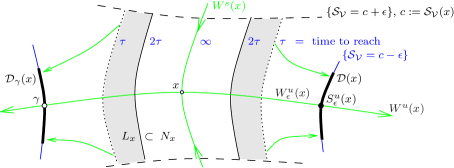
Figure 1: Conley pair $(N_{x},L_{x})$ for critical point $x$

Definition 1.6.

A Conley pair $(N,L)$ for a critical point $x$ of ${\mathcal{S}}_{\mathcal{V}}$ consists of an open subset $N\subset\Lambda M$ and a closed subset $L\subset N$ which satisfy

1. $x\in N\setminus L$

2. ${\rm cl\,}N\cap{\rm Crit}{\mathcal{S}}_{\mathcal{V}}=\{x\}$

3. $\gamma\in L$ and $\varphi_{[0,s]}\gamma\subset N\,\Rightarrow\,\varphi_{s}\gamma\in L$

4. $\gamma\in N$ and $\varphi_{T}\gamma\notin N\,\Rightarrow\,\exists\sigma\in(0,T):\varphi_{\sigma}\gamma\in L$ and $\varphi_{[0,\sigma]}\gamma\subset N$

In particular, conditions (i) and (ii) tell that $N$ is an open neighborhood of $x$ which contains no other critical points in its closure. Condition (iii) says that $L$ is positively invariant in $N$ and (iv) asserts that every semi-flow line which leaves $N$ goes through $L$ first. Hence we say that $L$ is an exit set of $N$.

Given a nondegenerate critical point $x$ of ${\mathcal{S}}_{\mathcal{V}}$, set $c:={\mathcal{S}}_{\mathcal{V}}(x)$. Borrowing from finite dimensions [16] we define the two sets

$$\begin{split}N_{x}=N_{x}^{{\varepsilon},\tau}:&=\left\{\gamma\in\Lambda M\mid\text{${\mathcal{S}}_{\mathcal{V}}(\gamma)<c+{\varepsilon}$, ${\mathcal{S}}_{\mathcal{V}}(\varphi_{\tau}\gamma)>c-{\varepsilon}$}\right\}_{x},\end{split}$$ (15)

where $\{\ldots\}_{x}$ denotes the path connected component that contains $x$, and

$$L_{x}=L_{x}^{{\varepsilon},\tau}:=\{\gamma\in N_{x}\mid{\mathcal{S}}_{\mathcal{V}}(\varphi_{2\tau}\gamma)\leq c-{\varepsilon}\}.$$ (16)

Note that $L_{x}$ is a relatively closed subset of the open subset $N_{x}$ of $\Lambda M$.

Theorem 1.7 (Conley pair).

The pair $(N_{x},L_{x})$ defined by (15-16) is a Conley pair for the nondegenerate critical point $x$ for all ${\varepsilon}>0$ small and $\tau>0$ large.

Theorem 1.7 holds for all ${\varepsilon}\in(0,\mu]$ and $\tau>\tau_{0}$ with $\mu$ and $\tau_{0}$ as in (H4) of Hypothesis 2.2. In this case all ascending/descending disks $W^{s,u}_{\varepsilon}$ and spheres $S^{s,u}_{\varepsilon}$ are manifolds.

Figure 1 shows a typical Conley pair, illustrates the exit set property of $L_{x}$, and indicates hypersurfaces which are characterized by the fact that each point reaches the level set $\{{\mathcal{S}}_{\mathcal{V}}=c-{\varepsilon}\}$ in the same time. The points on the stable manifold never reach level $c-{\varepsilon}$, so they are assigned the time label $\infty$. By the Backward $\lambda$-Lemma [30] locally near $x$ these hypersurfaces fiber over descending disks into diffeomorphic copies of the local stable manifold. This provides a foliation of small neighborhoods of $x$ the leaves of which, apriori, have no global meaning. It is the main content of Theorem C to express such neighborhoods and leaves in terms of (globally defined) level sets of the action functional. The difficulty being infinite dimension. Concerning the naming invariant stable foliation note the boldface ’stable’ above and a) below, whereas invariant refers to b). Parts c) and d) are quite useful as they allow to contract $N_{x}$ onto the ascending disk or even fit $N_{x}$ into any given neighborhood of $x$.

Theorem C (Invariant stable foliation).

Pick a nondegenerate critical point $x$ of ${\mathcal{S}}_{\mathcal{V}}$ and set $c:={\mathcal{S}}_{\mathcal{V}}(x)$. Then for every small ${\varepsilon}>0$ the following is true. Consider the descending sphere and the descending disk given by

$$S^{u}_{\varepsilon}(x):=W^{u}(x)\cap\{{\mathcal{S}}_{\mathcal{V}}=c-{\varepsilon}\},\quad W^{u}_{\varepsilon}(x):=W^{u}(x)\cap\{{\mathcal{S}}_{\mathcal{V}}>c-{\varepsilon}\}.$$ (17)

Pick a tubular neighborhood ${\mathcal{D}}(x)$ (associated to a radius $r$ normal disk bundle) over $S^{u}_{\varepsilon}(x)$ in the level hypersurface $\{{\mathcal{S}}_{\mathcal{V}}=c-{\varepsilon}\}$. Denote the fiber over $\gamma\in S^{u}_{\varepsilon}(x)$ by ${\mathcal{D}}_{\gamma}(x)$; see Figure 1. Then the following holds for every large $\tau>0$.

1. The set $N_{x}=N_{x}^{{\varepsilon},\tau}$ defined by (15) contains in its closure no critical points except $x$. Moreover, it carries the structure of a codimension-$k$ foliation whose leaves are parametrized by the $k$-disk $\varphi_{-\tau}W^{u}_{\varepsilon}(x)$ where $k$ is the Morse index of $x$. The leaf $N_{x}(x)$ over $x$ is the ascending disk $W^{s}_{\varepsilon}(x)$. The other leaves are the codimension-$k$ disks given by

   $$N_{x}(\gamma_{T})=\left({\varphi_{T}}^{-1}{\mathcal{D}}_{\gamma}(x)\cap\{{\mathcal{S}}_{\mathcal{V}}<c+{\varepsilon}\}\right)_{\gamma_{T}},\qquad\gamma_{T}:=\varphi_{-T}\gamma,$$

   whenever $T>\tau$ and $\gamma\in S^{u}_{\varepsilon}(x)$.

2. Leaves and semi-flow are compatible in the sense that

   $$z\in N_{x}(\gamma_{T})\quad\Rightarrow\quad\varphi_{\sigma}z\in N_{x}(\varphi_{\sigma}\gamma_{T})\quad\forall\sigma\in[0,T-\tau).$$

3. The leaves converge uniformly to the ascending disk in the sense that

   $${\rm dist}_{W^{1,2}}\left(N_{x}(\gamma_{T}),W^{s}_{\varepsilon}(x)\right)\leq e^{-T\frac{\lambda}{16}}$$ (18)

   for all $T>\tau$ and $\gamma\in S^{u}_{\varepsilon}(x)$; see (H4) below for $\lambda$. If $U$ is a neighborhood of the closure of $W^{s}_{\varepsilon}(x)$ in $\Lambda M$, then $N_{x}^{{\varepsilon},\tau_{*}}\subset U$ for some constant $\tau_{*}$.

4. Assume $U$ is a neighborhood of $x$ in $\Lambda M$. Then there are constants ${\varepsilon}_{*}$ and $\tau_{*}$ such that $N_{x}^{{\varepsilon}_{*},\tau_{*}}\subset U$.

Figure 2: Invariant foliation of $N=N^{{\varepsilon},\tau}$ in local coordinates of Hypothesis 2.2

Theorem D (Strong deformation retract).

Pick one of the Conley pairs $(N_{x},L_{x})$ in Theorem 1.7 and abbreviate by

$$N^{u}_{x}:=N_{x}\cap W^{u}(x),\qquad L^{u}_{x}:=L_{x}\cap W^{u}(x).$$

the corresponding parts in the unstable manifold. Then the pair of spaces $(N_{x},L_{x})$ strongly deformation retracts to $(N_{x}^{u},L_{x}^{u})$. Moreover, the latter pair consists of an open disk whose dimension $k$ is the Morse index of $x$ and an annulus which arises by removing a smaller open disk from the larger one.

Corollary 1.8.

Given a Conley pair $(N_{x},L_{x})$ as in Theorem 1.7, then

$${\rm H}_{\ell}(N_{x},L_{x})\cong\begin{cases}{\mathbb{Z}}&,\ell={\rm ind}_{\mathcal{V}}(x),\\ 0&,\text{otherwise.}\end{cases}$$ (19)

Proof.

Isomorphism (37). ∎

The task to prove (19) triggered the discovery of the Backward $\lambda$-Lemma in [30]. Luckily it was afterwards that we have been informed by Kell [7] that (19) should follow from Rybakowski’s theory [15]. The $\lambda$-Lemma, therefore Theorem C, both highly depend on finiteness of the Morse index. Furthermore, it is the proof of Theorem D in section 2.3 which requires the extension of the linearized graph maps in the Backward $\lambda$-Lemma [30] from $W^{1,2}$ to $L^{2}$; see Remark 2.12 and [28, Rmk. 1].

1.4 Past and future

The Morse complex goes back to the work of Thom [21], Smale [19, 20], and Milnor [9] in the 40’s, 50’s and 60’s, respectively. The geometric formulation in terms of flow trajectories was re-discovered by Witten in his influential 1982 paper [32]. He studied a supersymmetric quantum mechanical system related to the Laplacian $\Delta_{s}=d_{s}d_{s}^{*}+d_{s}^{*}d_{s}$ which involves the deformed Hodge differential $d_{s}=e^{-sf}de^{sf}$ acting on differential forms. Here $f:M\to{\mathbb{R}}$ denotes a Morse function on a closed Riemannian manifold $M$ and $s\geq 0$ is a real parameter. The Morse complex arises as the adiabatic limit of the quantum mechanical system, as the parameter $s$ tends to infinity. In the early 90’s the details of the construction have been worked out, among others, by Poźniak [14], by Schwarz [18] who developed the functional analytic framework, and by the author [25] who developed the dynamical systems framework. In the past decade Abbondandolo and Majer [1] extended the Morse complex to flows on Banach manifolds.

Morse homology for semi-flows was constructed only recently in [27, 28] where the functional analytic (moduli space) framework has been worked out for the heat flow. Being based on Sard’s theorem, the theory could be trivial. The present paper develops the dynamical systems framework and, above all, establishes non-triviality of the theory by calculating it in terms of singular homology.

Key tools are the invariant stable foliations provided by Theorem C which are of independent interest. For instance, the (non obvious) global stable manifold theorem for forward semi-flows will be a corollary of the main result of our forthcoming paper [23] whose base is Theorem C together with the pre-image idea – in a different guise though – which founded [31] and the present text.

An extremely rich source of semi-flows is obviously geometric analysis. For instance, although the present theory only deals with harmonic spheres of dimension one, it could be a first step in one of various possible directions.

Returning to present time, consider the finite dimensional case in which there is, of course, no need to consider semi-flow Morse homology. But there are (too) many choices which one can take while constructing the Morse complex. For instance, should one orient stable or unstable manifolds? Or even $M$ itself? Should we use the forward or the backward flow? The heat flow eliminates these questions alltogether – only the unstable manifolds are of finite dimension and there is no backward flow in general. We saw above that one even gets away with embedded ascending disks $W^{s}_{\varepsilon}(x)$, no manifold structure needed on all of $W^{s}(x)$. Furthermore, our construction of the natural isomorphism to singular homology applies correspondingly and is new in finite dimensions.

Finite Morse index is one of the most heavily used ingredients in this paper. Already the Backward $\lambda$-Lemma [31] hinges on it via well posedness of the mixed Cauchy problem. So does existence of the backward flow on unstable manifolds. That the action is bounded below and satisfies the Palais-Smale condition is also used frequently. The Abbondandolo-Majer extension of Morse-Smale to neighborhoods [1, Lemma 2.5] carries over to the present setup and is quite useful. Remarkably, in the very last step of our construction suddenly the need for a forward $\lambda$-Lemma arises; see Figure 14.

2 Conley pairs and stable foliations

In section 2 we study the heat flow locally near a given nondegenerate critical point $x$ of ${\mathcal{S}}_{\mathcal{V}}$ of Morse index $k$. The perturbation ${\mathcal{V}}$ is only required to satisfy axioms (V0)–(V3) in the notation of [28]. Throughout section 2 we use heavily results and notation of [31]. The reader may wish to have a copy at hand.

Remark 2.1 (Backward flow on unstable manifold).

The unstable manifold $W^{u}(x)$ carries a backward flow $\varphi_{-s}$. Thus the time-$s$-map $\varphi_{s}$ restricted to the unstable manifold is a diffeomorphism of $W^{u}(x)$ and its inverse is given by $\varphi_{-s}$. To see this recall that by definition, see e.g. [29, §6.1], each element $\gamma$ of $W^{u}(x)$ is of the form $u_{\gamma}(0,\cdot)$ where $u_{\gamma}:(-\infty,0]\times S^{1}\to M$ solves the heat equation (2) and $u_{\gamma}(s,\cdot)$ converges to $x$, as $s\to-\infty$. Given $s>0$, obviously $\varphi_{-s}\gamma:=u_{\gamma}(-s,\cdot)$ lies in the pre-image ${\varphi_{s}}^{-1}(\gamma)$ which contains no other element by backward unique continuation [29, Thm. 17].

Outline

In section 2.1 we define an open subset $N_{c}=N_{c}^{{\varepsilon},\tau}\subset\Lambda M$ associated to a critical value $c$ of the action and reals ${\varepsilon},\tau>0$. If the action of $x$ is $c$, then $N_{x}=N_{x}^{{\varepsilon},\tau}$ is the path connected component of $N_{c}^{{\varepsilon},\tau}$ that contains $x$. Lemma 2.6 asserts that $N_{x}$ intersects the stable manifold $W^{s}(x)$ in the ascending disk $W^{s}_{\varepsilon}(x)$ and the descending disk $W^{u}_{\varepsilon}(x)$ in the $k$-disk $\varphi_{-\tau}W^{u}_{\varepsilon}(x)$. The inclusions (21) suggest that $N_{x}$ contracts onto $x$, as ${\varepsilon}\to 0$ and $\tau\to\infty$. Thus by nondegeneracy of $x$ the closure of $N_{x}$ contains no critical point except $x$ whenever ${\varepsilon}>0$ is sufficiently small and $\tau>0$ is sufficiently large. Inspired by Conley [3] such $N_{x}$ is called an isolating block for $x$.

Section 2.2 shows that an isolating block $N_{x}$ is foliated by disks diffeomorphic to the ascending disk $W^{s}_{\varepsilon}(x)$ via the graph maps ${\mathcal{G}}^{T}_{\gamma}$ and ${\mathcal{G}}^{\infty}$ provided by the Backward $\lambda$-Lemma [31, Thm. 1] and the Local Stable Manifold Theorem [31, Thm. 3]. More precisely, the leaves of the foliation are parametrized by the elements of the $k$-disk $\varphi_{-\tau}W^{u}_{\varepsilon}(x)$. In particular, the leaf over its center $x$ is the ascending disk $W^{s}_{\varepsilon}(x)$. Furthermore, the heat flow $\varphi_{s}$ maps leaves to leaves and the isolating block $N_{x}$ contracts onto $W^{s}_{\varepsilon}(x)$, as $\tau\to\infty$.

In section 2.3 we extend the heat flow on the ascending disk $W^{s}_{\varepsilon}(x)$ artificially to the other leaves of the isolating block $N_{x}$ using the diffeomorphisms mentioned in the former paragraph. This way we prove that the part $N_{x}^{u}$ of $N_{x}$ in the unstable manifold is a strong deformation retract of $N_{x}$. This seems obvious. So why is there a long calculation? Because we need to make sure that the deformation takes place inside $N_{x}$ and the dimension of each leaf is infinite.

In section 2.4 we introduce the notion of an exit set $L_{x}=L_{x}^{{\varepsilon},\tau}$ associated to an isolating block $N_{x}=N_{x}^{{\varepsilon},\tau}$. The pair $(N_{x},L_{x})$ is called a Conley pair and we state and prove key properties that will be used in section 3. In particular we show that the homology of the pair $(N_{x},L_{x})$ coincides with the homology of the pair $({\mathbb{D}}^{k},\SS^{k-1})$ where $k$ is the Morse index of $x$ and $\SS^{k-1}$ denotes the boundary of the closed unit disk ${\mathbb{D}}^{k}\subset{\mathbb{R}}^{k}$.

Local coordinate setup and choices

Hypothesis 2.2.

Fix a perturbation ${\mathcal{V}}$ that satisfies the axioms (V0)–(V3) in [28] and a nondegenerate critical point $x$ of ${\mathcal{S}}_{\mathcal{V}}$ of Morse index $k$ and action $c$.

1. We use the local setup of [31], see Figure 4. Fix a local parametrization

   $$\Phi:\exp_{x}:X\supset{\mathcal{U}}\supset{\mathcal{B}}_{\rho_{0}}\to\Lambda M,\qquad X=T_{x}\Lambda M=W^{1,2}(S^{1},x^{*}TM),$$

   of a neighborhood of $x$ in $\Lambda M$ and consider the orthogonal splitting

   $$X=T_{x}W^{u}(x)\oplus T_{x}W^{s}_{\varepsilon}(x)=X^{-}\oplus X^{+}$$

   with corresponding orthogonal projections $\pi_{\pm}$. By a standard argument we assume that ${\mathcal{U}}$ is of the form $W^{u}\times{\mathcal{O}}^{+}$ where $W^{u}\subset X^{-}$ represents the unstable manifold near $x$ and ${\mathcal{O}}^{+}\subset X^{+}$ is an open ball about $0$. The constant $\rho_{0}>0$ is provided by [31, Hyp. 1] and ${\mathcal{B}}_{\rho_{0}}$ denotes the closed radius $\rho_{0}$ ball in $X$ centered at the origin.

   By $\phi$ we denote the local semi-flow on ${\mathcal{U}}$ which represents the heat flow with respect to $\Phi$; see [31, (5)]. In these coordinates $0\in X$ represents $x$ and ${\mathcal{S}}:={\mathcal{S}}_{\mathcal{V}}\circ\Phi^{-1}$ the action functional. In general, our coordinate notation will be the global notation with $x$ omitted, for example $W^{s}_{\varepsilon}$ abbreviates $\Phi^{-1}W^{s}_{\varepsilon}(x)$.

2. Due to nondegeneracy of the critical point $x$ we assume that the radius $\rho_{0}>0$ has been chosen sufficiently small such that the coordinate patch $\Phi({\mathcal{B}}_{\rho_{0}})$ about $x$ contains no other critical points.

3. Fix a constant $\mu>0$ sufficiently small such that the ascending disk $W^{s}_{2\mu}(x)$ defined by (6) and the descending disk $W^{u}_{2\mu}(x)$ defined by (17) are contained in the coordinate patch $\Phi({\mathcal{B}}_{\rho_{0}})$ and such that their closures are diffeomorphic to the closed unit disks in ${\mathbb{R}}^{k}$ and $X^{+}$, respectively; cf. Lemma 2.5 and Lemma 2.9.

4. The following are the hypotheses of Theorem C which allow to apply the Backward $\lambda$-Lemma [31, Thm. 1]. Fix an element $\lambda\in(0,d)$ in the spectral gap of the Jacobi operator $A_{x}$ associated to $x$. Pick ${\varepsilon}\in(0,\mu]$ where $\mu$ is the constant in (H3). Choose $r=r({\varepsilon})>0$ sufficiently small such that the tubular neighborhood ${\mathcal{D}}(x)$ associated to the radius $r$ normal disk bundle of the descending sphere $S^{u}_{\varepsilon}(x)$ in the level hypersurface $\{{\mathcal{S}}_{\mathcal{V}}=c-{\varepsilon}\}$ of the Hilbert manifold $\Lambda M$ exists and is contained in the coordinate patch $\Phi({\mathcal{B}}_{\rho_{0}})$. Denote the fiber over $\gamma\in S^{u}_{\varepsilon}(x)$ by ${\mathcal{D}}_{\gamma}(x)$; see Figures 1 or, in coordinates, Figure 2. Then there is a constant $\tau_{0}=\tau_{0}({\varepsilon},r,\lambda)>0$ such that the assertions of Theorem C hold true whenever $\tau>\tau_{0}$.

2.1 Isolating blocks

As some results in this section do not require nondegeneracy we use the notation $y$ for arbitrary critical points of ${\mathcal{S}}_{\mathcal{V}}$. In contrast $x$ always denotes the nondegenerate critical point that has been fixed at the very beginning of section 2.

Definition 2.3.

Assume ${\varepsilon}>0$ and $\tau>0$ are constants.

1. Given a critical value $c$ of the action functional ${\mathcal{S}}_{\mathcal{V}}$ consider the set 

   $$\begin{split}N_{c}=N_{c}^{{\varepsilon},\tau}:&=\left\{\gamma\in\Lambda M\mid\text{${\mathcal{S}}_{\mathcal{V}}(\gamma)<c+{\varepsilon}$, ${\mathcal{S}}_{\mathcal{V}}(\varphi_{\tau}\gamma)>c-{\varepsilon}$}\right\}\\ &=\{{\mathcal{S}}_{\mathcal{V}}<c+{\varepsilon}\}\cap\varphi^{-1}_{(\tau,\infty]}\{{\mathcal{S}}_{\mathcal{V}}=c-{\varepsilon}\}\end{split}$$ (20)

   where by definition $\varphi^{-1}_{\infty}\{{\mathcal{S}}_{\mathcal{V}}=c-{\varepsilon}\}$ denotes those points of $\Lambda M$ above action level $c-{\varepsilon}$ which never reach that level. 

2. Suppose $y$ is a critical point of action $c={\mathcal{S}}_{\mathcal{V}}(y)$. By $N_{y}=N_{y}^{{\varepsilon},\tau}$ we denote the path connected component of $N_{c}^{{\varepsilon},\tau}$ that contains $y$; compare (15).

3. Suppose $x$ is a nondegenerate critical point and there are no other critical points in the closure of $N_{x}^{{\varepsilon},\tau}$. Then $N_{x}^{{\varepsilon},\tau}$ is called an isolating block.

Figure 3 shows a set $N_{c}$ that consists of three path connected components one of which is an isolating block.

Figure 3: A set $N_{c}$ with three path connected components $N_{y}$, $A$, $N_{x}$

Lemma 2.4.

The set $N_{c}^{{\varepsilon},\tau}$ defined by (20) is an open subset of $\Lambda^{c+{\varepsilon}}M$ and contains all critical points with action values in the interval $(c-{\varepsilon},c+{\varepsilon})$.

Proof.

Openness is due to continuity of the action functional ${\mathcal{S}}_{\mathcal{V}}$ and Lipschitz continuity of the time-$s$-map $\varphi_{s}$ when restricted to sublevel sets. The latter follows from a mild extension of [27, Thm. 9.1.5]; see [24]. The second assertion is true since critical points of ${\mathcal{S}}_{\mathcal{V}}$ and fixed points of $\varphi_{s}$ coincide. ∎

Lemma 2.5 (Descending disks).

Given a nondegenerate critical point $x$ of ${\mathcal{S}}_{\mathcal{V}}$, there is a constant ${\varepsilon}_{0}>0$ such that the following is true. For each ${\varepsilon}\in(0,{\varepsilon}_{0}]$ the closure of the descending disk $W^{u}_{\varepsilon}(x)$ defined by (17) is diffeomorphic to the closed unit disk in ${\mathbb{R}}^{k}$ where $k$ is the Morse index of $x$. Furthermore, any open neighborhood $U$ of $x$ in the unstable manifold $W^{u}(x)$ contains the closure of some descending disk $W^{u}_{\varepsilon}(x)$.

Proof.

Unstable Manifold Theorem [28, Thm. 18] and Morse-Lemma [8]. ∎

Lemma 2.6.

Assume $N_{y}^{{\varepsilon},\tau}$ is given by Definition 2.3 (b), then

$$\begin{split}\delta<{\varepsilon}\;\;\Rightarrow\;\;N_{y}^{\delta,\tau}\subset N_{y}^{{\varepsilon},\tau},\qquad T>\tau\;\;\Rightarrow\;\;N_{y}^{{\varepsilon},T}\subset N_{y}^{{\varepsilon},\tau}.\end{split}$$ (21)

Assume $x$ is a nondegenerate critical point of ${\mathcal{S}}_{\mathcal{V}}$, then

$$\begin{split}N_{x}^{{\varepsilon},\tau}\cap W^{s}(x)&=W^{s}_{\varepsilon}(x),\\ N_{x}^{{\varepsilon},\tau}\cap W^{u}(x)&=\varphi_{-\tau}W^{u}_{\varepsilon}(x)\\ &=\{x\}\cup\bigcup_{T>\tau}\varphi_{-\tau}S^{u}_{\varepsilon}(x).\end{split}$$ (22)

for every ${\varepsilon}\in(0,{\varepsilon}_{0}]$ where ${\varepsilon}_{0}$ is given by the descending disk Lemma 2.5.

Proof.

The first inclusion in (21) is trivial and the second one follows from the fact that the action does not increase along heat flow trajectories.

Consider the first identity in (22). Since $W^{s}_{\varepsilon}(x):=W^{s}(x)\cap\{{\mathcal{S}}_{\mathcal{V}}<c+{\varepsilon}\}$ the inclusion “$\subset$” is trivial. To see “$\supset$” note that $W^{s}_{\varepsilon}(x)$ is a subset of $N_{c}$. Given $\gamma\in W^{s}_{\varepsilon}(x)$ the trajectory $\varphi_{[0,\infty]}\gamma$ connects $\gamma$ and $x$ in $W^{s}_{\varepsilon}(x)$, hence in $N_{c}$. Thus $\gamma$ lies in the component of $N_{c}$ that contains $x$.

Recall that $W^{u}_{\varepsilon}(x):=W^{u}(x)\cap\{{\mathcal{S}}_{\mathcal{V}}>c-{\varepsilon}\}$. By flow invariance of the unstable manifold $\varphi_{-\tau}W^{u}_{\varepsilon}(x)=W^{u}(x)\cap\{z\in\Lambda M\mid{\mathcal{S}}_{\mathcal{V}}(\varphi_{\tau}z)>c-{\varepsilon}\}\subset N_{c}$. Now the second identity in (22) follows by a similar argument as the first identity, just use backward trajectories. To see the third identity observe that any flow trajectory in $W^{s}(x)\setminus\{x\}$ hits $S^{u}_{\varepsilon}(x)$ precisely once. Obviously $W^{u}_{\varepsilon}(x)$ is diffeomorphic to its image under the diffeomorphism $\varphi_{-\tau}$ of $W^{u}(x)$. On the other hand, it is diffeomorphic to the open unit disk in ${\mathbb{R}}^{k}$ by the descending disk Lemma 2.5 where $k$ denotes the Morse index of $x$. ∎

Remark 2.7 (Open problem).

The inclusions (21) suggest that one could fit $N_{x}$ into any given neighborhood of $x$ by choosing ${\varepsilon}>0$ sufficiently small and $\tau>0$ sufficiently large. By Theorem C part (d) this is indeed possible. Can this also be achieved by shrinking only ${\varepsilon}$?

2.2 Stable foliations associated to level sets

Local non-intrinsic foliation

Assume (H1) and (H2) of Hypothesis 2.2. We start with an investigation of the foliation property provided by the Backward $\lambda$-Lemma [31, Thm. 1] for a disk family ${\mathcal{D}}=S^{u}_{\varepsilon}\times B_{\kappa}^{+}\subset{\mathcal{B}}_{\rho_{0}}$, not necessarily related to level sets, but which still has the no return property with respect to the local flow $\phi$, that is

$${\mathcal{D}}\cap{\phi_{s}}^{-1}{\mathcal{D}}=\emptyset$$

for all $s>0$ for which $\phi$ is defined.

Corollary 2.8 (to the Backward $\lambda$-Lemma [31, Thm. 1]).

Given (H1) and (H2), the assumptions of [31, Thm. 1], and the additional assumption that $({\mathcal{D}},\phi)$ has the no return property, then the following is true. Let ${\mathcal{G}},{\mathcal{G}}^{\infty}:{\mathcal{B}}^{+}\to X$ be the graph maps provided by Theorems 1 and 3 in [31], respectively. Then the subset

$$F=F^{{\varepsilon},T_{0}}:=\left({\rm im\,}{\mathcal{G}}\cup{\rm im\,}{\mathcal{G}}^{\infty}\right)\subset{\mathcal{B}}_{\rho_{0}}\subset{\mathcal{U}}$$

of the Banach space $X$ carries the structure of a codimension $k$ foliation; see Figure 2 for the part $N$ of $F$ below level $c+{\varepsilon}$. The leaves are given by the subset $F(0):={\mathcal{G}}^{\infty}({\mathcal{B}}^{+})$ of the local stable manifold $W^{s}(0,{\mathcal{U}})$, defined in Lemma 2.9, and by the graphs $F(\gamma_{T}):={\mathcal{G}}^{T}_{\gamma}({\mathcal{B}}^{+})$ for all $T>T_{0}$ and $\gamma\in S^{u}_{\varepsilon}$. Leaves and semi-flow are compatible in the sense that

$$z\in F(\gamma_{T})\quad\Rightarrow\quad\phi_{\sigma}z\in F(\phi_{\sigma}\gamma_{T})\qquad,\gamma_{T}:=\phi_{-T}\gamma={\mathcal{G}}^{T}_{\gamma}(0),$$

whenever the semi-flow trajectory from $z$ to $\phi_{\sigma}z$ remains inside $F$.

Proof of Corollary 2.8.

Assume that the leaves $F(\gamma_{T})$ and $F(\beta_{S})$ are disjoint whenever $\gamma_{T}\not=\beta_{S}$. Then the Lipschitz continuous $C^{1}$ maps ${\mathcal{G}}^{T}_{\gamma}:{\mathcal{B}}^{+}\to X$ and ${\mathcal{G}}^{\infty}:{\mathcal{B}}^{+}\to X$ endow $F$ with the structure of a codimension $k$ foliation.
To prove the assumption suppose $(T,\gamma)\not=(S,\beta)$. Because $T\geq T_{0}\geq T_{1}$, the endpoint conditions [31, (21)] are satisfied by the choice of $T_{1}$ in [31, (19)]. Assume by contradiction that ${\mathcal{G}}^{T}_{\gamma}(z_{+})={\mathcal{G}}^{S}_{\beta}(z_{+})=:z$ for some $z_{+}\in{\mathcal{B}}^{+}$. Then by [31, (31)] the point $z$ is the initial value of a heat flow trajectory $\xi^{T}$ ending at time $T$ on the fiber ${\mathcal{D}}_{\gamma}$ and also of a heat flow trajectory $\xi^{S}$ ending at time $S$ on ${\mathcal{D}}_{\beta}$. By uniqueness of the solution to the Cauchy problem [31, (5)] with initial value $z$ the two trajectories coincide until time $\min\{T,S\}$. If $T=S$, then $\gamma=\beta$ and we are done. Now assume without loss of generality that $T<S$, otherwise rename. Hence $\xi^{S}$ meets ${\mathcal{D}}_{\gamma}$ at time $T$ and ${\mathcal{D}}_{\beta}$ at the later time $S$. But this contradicts the no return property of ${\mathcal{D}}$.

We prove compatibility of leaves and semi-flow. The fixed point $0$ is semi-flow invariant. Its neighborhood $F(0)$ in the local stable manifold is trivially semi-flow invariant in the required sense, namely up to leaving $F(0)$. Pick $z\in F(\gamma_{T}):={\mathcal{G}}^{T}_{\gamma}({\mathcal{B}}^{+})$. By [31, (31)] the point $z$ is the initial value of a heat flow trajectory $\xi^{T}$ ending at time $T$ on the fiber ${\mathcal{D}}_{\gamma}$. Assume the image $\xi^{T}([0,T])=\phi_{[0,T]}z$ is contained in $F:={\rm im\,}{\mathcal{G}}\cup{\rm im\,}{\mathcal{G}}^{\infty}$. Pick $\sigma\in[0,T-T_{0}]$. This implies that $z_{+}:=\pi_{+}\phi_{\sigma}z\in{\mathcal{B}}^{+}$. The flow line $\phi_{[0,T-\sigma]}\phi_{\sigma}z$ runs from $\phi_{\sigma}z$ to $\phi_{T}z\in{\mathcal{D}}_{\gamma}$. Hence this flow line coincides with the fixed point $\xi_{\gamma,z_{+}}^{T-\sigma}$ of the strict contraction $\Psi_{\gamma,z_{+}}^{T-\sigma}$. But $\phi_{\sigma}z=\xi_{\gamma,z_{+}}^{T-\sigma}(0)$ is equal to ${\mathcal{G}}^{T-\sigma}_{\gamma}(z_{+})$ again by [31, (31)] and ${\mathcal{G}}^{T-\sigma}_{\gamma}({\mathcal{B}}^{+})=:F(\gamma_{T-\sigma})=F(\phi_{\sigma}\gamma_{T})$ by definition of $F$ and $\gamma_{T-\sigma}$. ∎

Ascending disks

Since nondegeneracy of $x$ is equivalent to a strictly positive spectral gap $d$, the following two results are based on the Palais-Morse Lemma [12] and the Local Stable Manifold Theorem [31, Thm. 3] whose neighborhood assertion uses the non-trivial fact that convergence implies exponential convergence.

Figure 4: The local ascending disk $W^{s}_{\varepsilon}(0,{\mathcal{U}})$ is a graph and equal to $W^{s}_{\varepsilon}$

Lemma 2.9 (Ascending disks).

Assume (H1) and (H2) of Hypothesis 2.2. The Local Stable Manifold Theorem [31, Thm. 3] provides the closed ball ${\mathcal{B}}^{+}$ about $0\in X^{+}$ of radius $r>0$. Then there is a constant ${\varepsilon}_{0}={\varepsilon}_{0}(r)>0$ such that the following is true whenever ${\varepsilon}\in(0,{\varepsilon}_{0}]$.

1. The local ascending disk defined by

   $$W^{s}_{\varepsilon}(0,{\mathcal{U}}):=W^{s}(0,{\mathcal{U}})\cap\{{\mathcal{S}}<{\mathcal{S}}(0)+{\varepsilon}\}$$

   is, firstly, a graph ${\mathcal{G}}^{\infty}({\mathcal{O}}^{+}_{\varepsilon})$ over the subset ${\mathcal{O}}^{+}_{\varepsilon}:=\pi_{+}W^{s}_{\varepsilon}(0,{\mathcal{U}})\subset{\mathcal{B}}^{+}$ which, secondly, is diffeomorphic to an open disk in $X^{+}$. Thirdly, that graph also coincides with the local stable manifold

   $$W^{s}(0,{\mathcal{N}}_{\varepsilon}):=\left\{z\in{\mathcal{N}}_{\varepsilon}\mid\text{$\phi(s,z)\in{\mathcal{N}}_{\varepsilon}$ $\forall s>0$ and $\lim_{s\to\infty}\phi(s,z)=0$}\right\}$$

   of the set ${\mathcal{N}}_{\varepsilon}:={\rm int\,}\,{\mathcal{B}}_{\rho_{0}}\cap{\pi_{+}}^{-1}{\mathcal{O}}^{+}_{\varepsilon}\subset{\mathcal{U}}$ illustrated in Figure 4.

2. Any neighborhood ${\mathcal{W}}$ of $0$ in $W^{s}(0,{\mathcal{U}})$ contains a local ascending disk.

3. The local coordinate representative $W^{s}_{\varepsilon}:=\Phi^{-1}W^{s}_{\varepsilon}(x)$ of the ascending disk $W^{s}_{\varepsilon}(x)$ defined by (6) coincides with the local ascending disk $W^{s}_{\varepsilon}(0,{\mathcal{U}})$.

Corollary 2.10.

In the notation of Lemma 2.9 assume that ${\mathcal{N}}\subset{\mathcal{U}}$ is an open subset which contains the hyperbolic fixed point $0$. Then the local stable manifold $W^{s}(0,{\mathcal{N}})$ is an open neighborhood of $0$ in $W^{s}(0,{\mathcal{U}})$.

Proof of Lemma 2.9.

(Ascending disks). By the Local Stable Manifold Theorem [31, Thm. 3] a neighborhood of $0$ in $W^{s}(0,{\mathcal{U}})$, say ${\mathcal{W}}\subset{\rm range\,}{\mathcal{G}}$, is embedded in $\Lambda M$ and its tangent space at $0$ is $X^{+}=\pi_{+}(X)$. Observe that the restriction $f:={\mathcal{S}}|$ of the action to ${\mathcal{W}}$ is a Morse function. Apply the Palais-Morse Lemma [12] to obtain a coordinate system on ${\mathcal{W}}$ (choose ${\mathcal{W}}$ smaller if necessary) modelled on $T_{0}{\mathcal{W}}=X^{+}$ and such that

$$f(y)=\sum_{j=1}^{\infty}\lambda_{k+j}y_{j}^{2}$$

for every $y\in{\mathcal{W}}$. Here $y=\sum_{j=1}^{\infty}y_{j}\xi_{k+j}$ and $0<\lambda_{k+1}<\lambda_{k+2}<\ldots$ are the positive eigenvalues of the Jacobi operator $A$ associated to the critical point $0$ of ${\mathcal{S}}$ with corresponding normalized eigenvectors $\xi_{k+j}$; see e.g. [31, (2)].

In these coordinates the local ascending disk $W^{s}_{\varepsilon}(0,{\mathcal{U}})$ takes the form of an open ellipse in $X^{+}$ which is given by

$$\begin{split}{\mathcal{E}}_{\varepsilon}&:={\mathcal{E}}\left(a_{1},a_{2},\ldots\right)=\biggl{\{}y\in X^{+}\colon\sum_{j=1}^{\infty}\lambda_{k+j}y_{j}^{2}<{\varepsilon}\biggr{\}}\subset{\mathcal{O}}^{+}_{R}\\ a_{j}&:=\sqrt{\frac{{\varepsilon}}{\lambda_{k+j}}}\end{split}$$

and contained in the open ball $\dot{\mathcal{B}}^{+}_{R}\subset X^{+}$ of radius $R=a_{1}({\varepsilon})$. Since any neighborhood of $0$ contains a ball of sufficiently small radius this proves part (ii).

To prove (i) fix the radius ${\varepsilon}_{0}>0$ sufficiently small such that the open ball $\dot{\mathcal{B}}^{+}_{{\varepsilon}_{0}}$ is contained, firstly, in the domain of our Palais-Morse parametrization, secondly, in the Palais-Morse representative of ${\mathcal{W}}$ and, thirdly, in the Palais-Morse representative of the ball ${\mathcal{B}}^{+}\subset X^{+}$ of radius $r>0$. The second assertion in part (i) follows since $\dot{\mathcal{B}}^{+}_{{\varepsilon}_{0}}$ represents the manifold $W^{s}_{{\varepsilon}_{0}}(0,{\mathcal{U}})$ which is diffeomorphic under $\pi_{+}$ to

$${\mathcal{O}}^{+}_{{\varepsilon}_{0}}:=\pi_{+}W^{s}_{{\varepsilon}_{0}}(0,{\mathcal{U}})\subset{\mathcal{B}}^{+}.$$

Here the diffeomorphism property follows from the fact that $W^{s}_{{\varepsilon}_{0}}(0,{\mathcal{U}})$ is tangent to $X^{+}$ at $0$ and by choosing ${\varepsilon}_{0}>0$ smaller, if necessary. The tangency argument also justifies the assumption that $W^{s}_{{\varepsilon}_{0}}(0,{\mathcal{U}})\subset{\rm int\,}\,{\mathcal{B}}_{\rho_{0}}$, otherwise choose ${\varepsilon}_{0}>0$ smaller. The same arguments work for each ${\varepsilon}\in(0,{\varepsilon}_{0}]$ and ${\mathcal{G}}({\mathcal{O}}^{+}_{\varepsilon})$ is well defined.

To prove the remaining assertions one and three in (i) we show that

$${\mathcal{G}}({\mathcal{O}}^{+}_{\varepsilon})\subset W^{s}(0,{\mathcal{N}}_{\varepsilon})=W^{s}_{\varepsilon}(0,{\mathcal{U}})\subset{\mathcal{G}}({\mathcal{O}}^{+}_{\varepsilon}),\quad{\mathcal{N}}_{\varepsilon}:={\rm int\,}\,{\mathcal{B}}_{\rho_{0}}\cap{\pi_{+}}^{-1}{\mathcal{O}}^{+}_{\varepsilon},$$ (23)

whenever ${\varepsilon}\in(0,{\varepsilon}_{0}]$. To understand the middle identity observe that the inclusion ’$\subset$’ is obvious since ${\mathcal{N}}_{\varepsilon}\subset{\mathcal{B}}_{\rho_{0}}\subset{\mathcal{U}}$. To see the reverse ’$\supset$’ note that

$$W^{s}_{\varepsilon}(0,{\mathcal{U}})\subset\left({\rm int\,}\,{\mathcal{B}}_{\rho_{0}}\cap{\pi_{+}}^{-1}\pi_{+}W^{s}_{\varepsilon}(0,{\mathcal{U}})\right)=:{\mathcal{N}}_{\varepsilon}.$$

By semi-flow invariance of local ascending disks the elements of $W^{s}_{\varepsilon}(0,{\mathcal{U}})$ converge to $0$ without leaving $W^{s}_{\varepsilon}(0,{\mathcal{U}})$, hence without leaving ${\mathcal{N}}_{\varepsilon}$. But this means that $W^{s}_{\varepsilon}(0,{\mathcal{U}})\subset W^{s}_{\varepsilon}(0,{\mathcal{N}}_{\varepsilon})$. To prove the second inclusion in (23) observe that ${\mathcal{N}}:={\mathcal{G}}({\mathcal{O}}^{+}_{{\varepsilon}_{0}})$ is a neighborhood of $0$ in $W^{s}(0,{\mathcal{U}})$. Apply part (ii) proved above and readjust ${\varepsilon}_{0}$, if necessary. This proves that $W^{s}_{\varepsilon}(0,{\mathcal{U}})\subset{\mathcal{G}}({\mathcal{O}}^{+}_{\varepsilon})$. To prove the first inclusion in (23) pick $z\in{\mathcal{G}}({\mathcal{O}}^{+}_{\varepsilon})$, that is

$$z=(Gz_{+},z_{+})={\mathcal{G}}(z_{+})\in{\mathcal{G}}({\mathcal{O}}^{+}_{\varepsilon})$$

for some $z_{+}\in{\mathcal{O}}^{+}_{\varepsilon}$. To see that $z\in W^{s}_{\varepsilon}(0,{\mathcal{U}})$ consider the (unique) element $z_{*}$ of $W^{s}_{\varepsilon}(0,{\mathcal{U}})$ which projects under the diffeomorphism $\pi_{+}:W^{s}_{\varepsilon}(0,{\mathcal{U}})\to{\mathcal{O}}^{+}_{\varepsilon}$ to $z_{+}$. Since we already know that $W^{s}_{\varepsilon}(0,{\mathcal{U}})\subset{\mathcal{G}}({\mathcal{O}}^{+}_{\varepsilon})$ the point $z_{*}\in W^{s}_{\varepsilon}(0,{\mathcal{U}})$ is of the form $z_{*}={\mathcal{G}}(z_{+})$. But ${\mathcal{G}}(z_{+})=z$.

The key information to prove part (iii) is the fact shown above using the Palais-Morse lemma, namely that the local ascending disk $W^{s}_{\varepsilon}(0,{\mathcal{U}})$ is contained in the interior of the ball ${\mathcal{B}}_{\rho_{0}}$ which itself is contained in the domain ${\mathcal{U}}$ of the parametrization $\Phi$. But $\Phi$ intertwines the local semi-flows $\phi_{s}$ on ${\mathcal{U}}$ and $\varphi_{s}$ on $\Phi({\mathcal{U}})$ by its very definition; cf. [31, (5)]. ∎

Proof of Corollary 2.10.

Obviously $0\in W^{s}(0,{\mathcal{N}})\subset W^{s}(0,{\mathcal{U}})$. It remains to show that the subset $W^{s}(0,{\mathcal{N}})$ of $W^{s}(0,{\mathcal{U}})$ is open. Fix $z\in W^{s}(0,{\mathcal{N}})\subset{\mathcal{N}}$. It suffices to prove existence of an open ball ${\mathcal{O}}(z)\subset{\mathcal{U}}$ about $z$ such that the (open) subset ${\mathcal{O}}(z)\cap W^{s}(0,{\mathcal{U}})$ of $W^{s}(0,{\mathcal{U}})$ is contained in $W^{s}(0,{\mathcal{N}})$. Assume by contradiction that no such ball exists. In this case there is a sequence $(z_{i})$ contained in $W^{s}(0,{\mathcal{U}})$ and in ${\mathcal{N}}$, but disjoint to $W^{s}(0,{\mathcal{N}})$, and which converges to $z$ in the $W^{1,2}$ topology. Consequently for each $z_{i}$ there is a time $s_{i}>0$ such that $\phi_{s_{i}}z_{i}\notin{\mathcal{N}}$. Taking subsequences, if necessary, we distinguish two cases:
In case one the sequence $(s_{i})$ is contained in some bounded interval $[0,T]$. Now $\phi$ restricted to a sublevel set is uniformly Lipschitz on a fixed interval $[0,T]$ by a slightly improved version of [27, Thm. 9.15]; see [24]. Thus the sequence of continuous maps $[0,T]\to{\mathcal{U}}:s\mapsto w_{z_{i}}(s):=\phi_{s}z_{i}$ converges uniformly to the map $w_{z}:[0,T]\to{\mathcal{N}}\subset{\mathcal{U}}$. But this implies that the image of $w_{z_{i}}$ is also contained in ${\mathcal{N}}$ for all sufficiently large $i$ which contradicts the fact that $\phi_{s_{i}}z_{i}\notin{\mathcal{N}}$.
In case two $s_{i}\to\infty$, as $i\to\infty$. By openness of ${\mathcal{N}}$ there is a sufficiently small open ball ${\mathcal{O}}_{\rho}$ of radius $\rho$ about $0\in{\mathcal{U}}$ which is contained in ${\mathcal{N}}$. By Lemma 2.9 (ii) there is a local ascending disk $W^{s}_{\varepsilon}(0,{\mathcal{U}})$ contained in the open neighborhood ${\mathcal{W}}:=W^{s}(0,{\mathcal{U}})\cap{\mathcal{O}}_{\rho}$ of $0$ in $W^{s}(0,{\mathcal{U}})$. Fix $\tau>0$ large such that $\phi(\tau,z)\in W^{s}_{{\varepsilon}/2}(0,{\mathcal{U}})$. Then the following is true for every sufficiently large $i$: The point $\phi(\tau,z_{i})$ lies in $W^{s}_{\varepsilon}(0,{\mathcal{U}})$ by continuity of $\phi$. But $W^{s}_{\varepsilon}(0,{\mathcal{U}})$ is semi-flow invariant and contained in ${\mathcal{O}}_{\rho}\subset{\mathcal{N}}$. So $\phi(s,z_{i})\in{\mathcal{N}}$ for $s\in[\tau,\infty)$ which contradicts $s_{i}\to\infty$. ∎

Proof of Theorem C – intrinsic foliation

Assume Hypothesis 2.2 (H1–H4). In particular, by definition of $\mu$ in (H3) both the descending disk $W^{u}_{2\mu}(x)$ and the ascending disk $W^{s}_{2\mu}(x)$ are manifolds and lie in the coordinate patch $\Phi({\mathcal{B}}_{\rho_{0}})$ about the nondegenerate critical point $x$ of Morse index $k$. The Local Stable Manifold Theorem [31, Thm. 3] provides the graph map ${\mathcal{G}}^{\infty}:{\mathcal{B}}^{+}\to X$ defined on the closed ball ${\mathcal{B}}^{+}={\mathcal{B}}^{+}_{r}$ about $0\in X^{+}$ whose radius $r$ we write in the form

$$r=:2R.$$ (24)

Again by [31, Thm. 3] the set ${\mathcal{N}}:={\mathcal{G}}^{\infty}(\dot{\mathcal{B}}_{R}^{+})$ is an open neighborhood of $0$ in the local stable manifold $W^{s}(0,{\mathcal{U}})$. Thus ${\mathcal{N}}$ contains an ascending disk by the ascending disk Lemma 2.9 (ii). Choosing $\mu>0$ smaller, if necessary, we assume without loss of generality that there is the inclusion of the ascending disk coordinate representative

$$W^{s}_{\mu}\subset{\mathcal{N}}:={\mathcal{G}}^{\infty}(\dot{\mathcal{B}}_{R}^{+}).$$ (25)

The coordinate representative ${\mathcal{D}}$ of the tubular neighborhood ${\mathcal{D}}(x)$ intersects the unstable manifold transversally in $S^{u}_{\varepsilon}$. Use the implicit function theorem, if necessary, to modify the coordinate system locally near ${\mathcal{D}}$ to make sure that ${\mathcal{D}}$ is an open neighborhood of $S^{u}_{\varepsilon}$ in $S^{u}_{\varepsilon}\times X^{+}$. Pick a radius $\varkappa\in(0,\rho_{0})$ sufficiently small such that $S^{u}_{\varepsilon}\times{\mathcal{B}}_{\varkappa}^{+}$ is contained in ${\mathcal{D}}$ and in ${\mathcal{B}}_{\rho_{0}}$. Next diminish ${\mathcal{D}}$ setting

$${\mathcal{D}}:=S^{u}_{\varepsilon}\times{\mathcal{B}}_{\varkappa}^{+},\qquad{\mathcal{D}}\cap{\rm Crit}=\emptyset,$$ (26)

where the latter observation holds by (H2). Since ${\mathcal{D}}$ is contained in an action level set and $\phi$ is a gradient semi-flow, the pair $({\mathcal{D}},\phi)$ has the no return property. Consider the constant $T_{0}=T_{0}(x,\lambda,{\varepsilon},\varkappa)>0$ and the graph maps ${\mathcal{G}}^{T}_{\gamma}$ provided by the Backward $\lambda$-Lemma [31, Thm. 1] for all $T\geq T_{0}$ and elements $\gamma$ of the descending $(k-1)$-disk $S^{u}_{\varepsilon}$; see Figure 5.

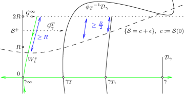
Figure 5: The disk ${\mathcal{G}}^{T}_{\gamma}({\mathcal{B}}^{+})\cap\{{\mathcal{S}}<c+{\varepsilon}\}=\left({\phi_{T}}^{-1}{\mathcal{D}}_{\gamma}\cap\{{\mathcal{S}}<c+{\varepsilon}\}\right)_{\gamma_{T}}$

Step 1. (Graphs) There is a constant $T_{1}\geq T_{0}$ such that the following is true. Assume $T\in[T_{1},\infty]$ and $\gamma\in S^{u}_{\varepsilon}$. Then the set ${\mathcal{G}}^{T}_{\gamma}({\mathcal{B}}^{+})\cap\{{\mathcal{S}}<c+{\varepsilon}\}$ is diffeomorphic to the open unit disk in $X^{+}$.

Proof.

Case 1. ($T=\infty$) The graph ${\mathcal{G}}^{\infty}({\mathcal{B}}^{+})$ – which is a neighborhood of $0$ in the local stable manifold $W^{s}(0,{\mathcal{U}})$ by the Local Stable Manifold Theorem [31, Thm. 3] – intersects the sublevel set $\{{\mathcal{S}}<c+{\varepsilon}\}$ transversally in the ascending disk $W^{s}_{\varepsilon}$. But $W^{s}_{\varepsilon}$ is diffeomorphic to the open ${\varepsilon}$-disk in $X^{+}$ by the Palais-Morse lemma using the fact that the positive part of the spectrum of the Jacobi operator $A_{x}$ is bounded away from zero (by its smallest positive eigenvector $\lambda_{k+1}$). For the above assertions see Lemma 2.9.

Case 2. ($T<\infty$) By the Backward $\lambda$-Lemma [31, Thm. 1] the family of disks $T\mapsto{\mathcal{G}}^{T}_{\gamma}({\mathcal{B}}^{+})$ is uniformly $C^{1}$ close to the disk ${\mathcal{G}}^{\infty}({\mathcal{B}}^{+})$. Transversality of the intersection with $\{{\mathcal{S}}<c+{\varepsilon}\}$ is automatic since the sublevel set is an open subset of the loop space. However, since the graphs ${\mathcal{G}}^{T}_{\gamma}({\mathcal{B}}^{+})$ are manifolds with boundaries we need to make sure that these boundaries stay away from $\{{\mathcal{S}}<c+{\varepsilon}\}$ in order to conclude that any intersection ${\mathcal{G}}^{T}_{\gamma}({\mathcal{B}}^{+})\cap\{{\mathcal{S}}<c+{\varepsilon}\}$ is diffeomorphic to the intersection ${\mathcal{G}}^{\infty}({\mathcal{B}}^{+})\cap\{{\mathcal{S}}<c+{\varepsilon}\}=W^{s}_{\varepsilon}$. But the latter is diffeomorphic to the open unit disk in $X^{+}$ by Case 1.
Concerning boundaries recall that $\pi_{+}{\mathcal{G}}^{\infty}({\mathcal{B}}^{+})=\pi_{+}{\mathcal{G}}^{T}_{\gamma}({\mathcal{B}}^{+})={\mathcal{B}}^{+}={\mathcal{B}}^{+}_{2R}$. Here the second identity holds by step 5 in the proof of [31, Thm. 1]. On the other hand, the topological boundary of $W^{s}_{\varepsilon}$ projects into ${\mathcal{B}}^{+}_{R}$ by the choice of $\mu$ in (25); see Figure 5. Thus the distance between the boundary of ${\mathcal{G}}^{\infty}({\mathcal{B}}^{+})$ and the intersection ${\mathcal{G}}^{\infty}({\mathcal{B}}^{+})\cap\{{\mathcal{S}}<c+{\varepsilon}\}=W^{s}_{\varepsilon}$ is at least $R$. Since ${\mathcal{G}}^{T}_{\gamma}\to{\mathcal{G}}^{\infty}$, as $T\to\infty$, uniformly on ${\mathcal{B}}^{+}$ and uniformly in $\gamma\in S^{u}_{\varepsilon}$, there is a time $T_{1}>0$ such that the distance between the boundary of ${\mathcal{G}}^{T}_{\gamma}({\mathcal{B}}^{+})$ and the intersection ${\mathcal{G}}^{T}_{\gamma}({\mathcal{B}}^{+})\cap\{{\mathcal{S}}<c+{\varepsilon}\}$ is at least $R/2$ for all $\gamma$ and $T\geq T_{1}$. ∎

Step 2. (Pre-Images) For all $T\geq T_{1}$ and $\gamma\in S^{u}_{\varepsilon}$ the following is true.

1. The disk ${\mathcal{G}}^{T}_{\gamma}({\mathcal{B}}^{+})\cap\{{\mathcal{S}}<c+{\varepsilon}\}=:D$ is a neighborhood of $\gamma_{T}$ in the pathwise connected component $P_{\gamma_{T}}$ of the set $P:={\phi_{T}}^{-1}{\mathcal{D}}_{\gamma}\cap\{{\mathcal{S}}<c+{\varepsilon}\}$.

2. The disk ${\mathcal{G}}^{T}_{\gamma}({\mathcal{B}}^{+})\cap\{{\mathcal{S}}<c+{\varepsilon}\}$ equals $P_{\gamma_{T}}:=\left({\phi_{T}}^{-1}{\mathcal{D}}_{\gamma}\cap\{{\mathcal{S}}<c+{\varepsilon}\}\right)_{\gamma_{T}}$.

Proof.

a) That $\gamma_{T}$ is contained in $P$ is obvious and that it is contained in $D$ is asserted by the Backward $\lambda$-Lemma [31, Thm. 1]. To see that $D\subset P_{\gamma_{T}}$ pick $z\in D$. Then the heat flow takes $z$ in time $T$ into ${\mathcal{D}}_{\gamma}$ by definition of ${\mathcal{G}}^{T}_{\gamma}$ and the identity [31, (31)]. Hence $z\in P$ and therefore $D\subset P$. Thus to prove that $D\subset P_{\gamma_{T}}$ it suffices to show that $z$ path connects to $\gamma_{T}$ inside $D$. But this is trivial, because $D$ is diffeomorphic to a disk by Step 1. To see the neighborhood property of $D$ pick $z\in P_{\gamma_{T}}$ and connect $z$ to $\gamma_{T}$ inside $P$ through a continuous path. Of course, since $\pi_{+}\gamma_{T}=0$ the elements of the path near $\gamma_{T}$ project under $\pi_{+}$ into ${\mathcal{B}}^{+}$ and are therefore in the image of the map ${\mathcal{G}}^{T}_{\gamma}$ defined by [31, (25)].

b) By part a) it remains to prove the inclusion ’$\supset$’. Pick $z\in P_{\gamma_{T}}$ and connect $z$ to $\gamma_{T}$ inside $P$ through a continuous path. Note that all points on this path have action strictly less than $c+{\varepsilon}$. Now if z was not in the disk $D$, this path would have to cross the topological boundary of $D$ by the neighborhood property in a). But ${\partial}D$ is contained in the level set $\{{\mathcal{S}}=c+{\varepsilon}\}$. Contradiction. ∎

Step 3. Set $\tau_{0}:=2T_{1}$. Assume from now on that $\tau>\tau_{0}$. Recall that Corollary 2.8 provides the codimension $k$ foliation $F=F^{{\varepsilon},\tau}:={\rm im\,}{\mathcal{G}}^{(\tau,\infty]}$. Then

$$A:=F^{{\varepsilon},\tau}\cap\{{\mathcal{S}}<c+{\varepsilon}\}=N^{{\varepsilon},\tau}=:N,$$

that is the part $A$ below level $c+{\varepsilon}$ of the foliation $F^{{\varepsilon},\tau}$ is equal to the coordinate representative of the set $N_{x}^{{\varepsilon},\tau}$ defined by (15); see Figure 6. The point is that $A$ is essentially the image of a family of maps, but the definition of $N$ requires each point being path connectable to $0$.

Figure 6: The set $A$ in step 3 with neighborhood $A\cup I\cup II$

Proof.

$A\subset N$: Pick $z\in A$. Then ${\mathcal{S}}(z)<c+{\varepsilon}$ and $z$ is of the form ${\mathcal{G}}^{T}_{\gamma}(z_{+})$ for some time $T\in(\tau,\infty]$ and elements $\gamma\in S^{u}_{\varepsilon}$ and $z_{+}\in{\mathcal{B}}^{+}$. But ${\mathcal{G}}^{T}_{\gamma}(z_{+})=\xi^{T}_{\gamma,z_{+}}(0)$ by [31, (31)] and therefore $z$ runs under the heat flow in time $T>\tau$ into the subset ${\mathcal{D}}$ of the level set $\{{\mathcal{S}}=c-{\varepsilon}\}$. Thus ${\mathcal{S}}(\phi_{\tau}z)>c-{\varepsilon}$ by the downward gradient flow property and the fact that by (26) there is no critical point of ${\mathcal{S}}$ on ${\mathcal{D}}$. To conclude the proof that $z\in N$ it remains to show that there is a continuous path in $N$ between $z$ and $0$. By Step 1 the set ${\mathcal{G}}^{T}_{\gamma}({\mathcal{B}}^{+})$ is a disk and therefore path connected. Connect $z$ and $\gamma_{T}$ by a continuous path in this disk. Any point on this path lies in $\{{\mathcal{S}}<c+{\varepsilon}\}\cap\{{\mathcal{S}}(\phi_{\tau}\cdot)>c-{\varepsilon}\}$ by the argument just given for $z$. Connect $\gamma_{T}$ and $\gamma_{\infty}=0$ by the obvious backward flow line. Repeat the argument for the points on this second path. Hence we have connected $z$ and $0$ by a continuous path in $N$.

$A\supset N$: Assuming $z\notin A$ we prove that $z\notin N$. To be not in $A$ we distinguish three cases; see Figure 6. In case one $z$ lies in the set $I:={\rm im\,}{\mathcal{G}}^{(\tau/2,\tau]}\cap\{{\mathcal{S}}<c+{\varepsilon}\}$. But this means that $z$ reaches level $c-{\varepsilon}$ in some time $T\leq\tau$. Hence ${\mathcal{S}}(\phi_{\tau})\leq c-{\varepsilon}$ and therefore $z\notin N$. In case two $z$ lies in the set $II:=\{{\mathcal{S}}\geq c+{\varepsilon}\}$ which is obviously disjoint to $N$. In case three $z$ lies in the set $III:=\{{\mathcal{S}}<c+{\varepsilon}\}\cap\{{\mathcal{S}}(\phi_{\tau/2}\cdot)\leq c-{\varepsilon}\}$ shown in Figure 6. Assume by contradiction $z\in N$. Then $z$ and $0$ connect through a continuous path in $N$. Note that $0\in A$ since ${\mathcal{G}}^{\infty}(0)=0$. Since $A\cup I\cup II$ is a neighborhood of $A$, the path must run through $I\cup II$ which is impossible by cases one and two. ∎

Proof of a). (Foliation).

By Step 3 and Corollary 2.8 there are the inclusions $N^{{\varepsilon},\tau}\subset F^{{\varepsilon},\tau}\subset{\mathcal{B}}_{\rho_{0}}$. But by (H2) the ball ${\mathcal{B}}_{\rho_{0}}$ contains no critical point except the origin. Thus $N_{x}$ is an isolating block for $x$; this also follows from part d).

By Corollary 2.8 the set $F=F^{{\varepsilon},\tau}$ carries the structure of a codimension $k$ foliation. By Step 3 the set $N=N^{{\varepsilon},\tau}$ is an open subset of $F$ and therefore inherits the foliation structure of $F$. We define the leaves of $N$ by $N(0):=F(0)\cap\{{\mathcal{S}}<c+{\varepsilon}\}={\mathcal{G}}^{\infty}({\mathcal{B}}^{+})\cap\{{\mathcal{S}}<c+{\varepsilon}\}$ and by $N(\gamma_{T}):=F(\gamma_{T})\cap\{{\mathcal{S}}<c+{\varepsilon}\}={\mathcal{G}}^{T}_{\gamma}({\mathcal{B}}^{+})\cap\{{\mathcal{S}}<c+{\varepsilon}\}$ where $T\in(\tau,\infty)$ and $\gamma\in S^{u}_{\varepsilon}$. The second identities are just by definition of $F(0)$ and $F(\gamma_{T})$ in Corollary 2.8. Since the right hand sides are disks by Step 1 the leaves of $N$ are indeed parametrized by the disjoint union of $\{0\}$ and $(\tau_{0},\infty)\times S^{u}_{\varepsilon}$. Hence the leaves of $N$ and $F$ are in 1-1 correspondence. They are of the asserted form by Step 2 b). ∎

Proof of b). (Compatibility of leaves and semi-flow).

That leaves and semi-flow are compatible follows from Corollary 2.8 as soon as we prove that semi-flow trajectories starting and ending in $N=N^{{\varepsilon},\tau}$ cannot leave $N$ (hence not $F$) at any time in between. To see this decompose the (topological) boundary of the set $N=F\cap\{{\mathcal{S}}<c+{\varepsilon}\}$ into the top part ${\partial}^{+}N$ which lies in the level set $\{{\mathcal{S}}=c+{\varepsilon}\}$ and its complement the side part ${\partial}^{-}N=\bigcup_{\gamma\in S^{u}_{\varepsilon}}{\mathcal{G}}^{\tau}_{\gamma}({\mathcal{B}}^{+})\cap\{{\mathcal{S}}<c+{\varepsilon}\}$ as illustrated by Figure 7 below. The downward gradient property implies, firstly, that ${\partial}^{+}N$ cannot be reached from lower action levels (thus not from $N$) and, secondly, that ${\partial}^{-}N$ cannot be crossed twice. To prove the latter assume by contradiction that there are two elements $z_{1}\not=z_{2}$ of

$${\partial}^{-}N=\left({\phi_{\tau}}^{-1}{\mathcal{D}}\cap\{{\mathcal{S}}<c+{\varepsilon}\}\right)_{\phi_{-\tau}S^{u}_{\varepsilon}}$$

that lie on the same semi-flow trajectory starting at, say $z_{1}$. Now on one hand, the time needed from either one element to ${\mathcal{D}}$ is $\tau$. On the other hand, getting from $z_{1}$ to $z_{2}$ requires the extra time $T>0$. By uniqueness of the solution to the Cauchy problem it follows that $\tau+T=\tau$ which contradicts $T>0$. ∎

Proof of c). (Uniform convergence of leaves).

Uniform and exponential convergence of leaves follows from the exponential estimate in [31, Thm. 1], in which we can actually eliminate the constant $\rho_{0}$ by choosing $T_{0}$ larger, together with the inclusion $N(\gamma_{T})={\mathcal{G}}^{T}_{\gamma}({\mathcal{B}}^{+})\cap\{{\mathcal{S}}_{\mathcal{V}}<c+{\varepsilon}\}\subset{\mathcal{G}}^{T}_{\gamma}({\mathcal{B}}^{+})$ and the corresponding one for $T=\infty$; for the identity see proof of a). This proves (18). Given $U$ as in the second assertion, pick a $\delta$-neighborhood $U_{\delta}\subset\Phi^{-1}(U)$ of $W^{s}_{\varepsilon}$ in ${\mathcal{B}}_{\rho_{0}}$ for some $\delta\in(0,1)$. Estimate (18) shows that $N^{{\varepsilon},\tau_{*}}\subset U_{\delta}$ whenever $\tau_{*}>-\frac{16}{\lambda}\ln\delta$. ∎

Proof of d). (Localization of $N_{x}$).

The two key ingredients are that the ascending disk $W^{s}_{\varepsilon}(x)$ localizes near $x$ for small ${\varepsilon}$ by the Palais-Morse Lemma and that the isolating block $N_{x}^{{\varepsilon},\tau}$ contracts onto $W^{s}_{\varepsilon}(x)$ by estimate (18) in part c).

Replacing the neighborhood $U$ of $x$ in $\Lambda M$ by a smaller neighborhood, if necessary, we solve the problem in the local coordinate patch $\Phi({\mathcal{B}}_{\rho_{0}})$ about $x$. Thus we assume that $U$ is a neighborhood of $0$ in ${\mathcal{B}}_{\rho_{0}}\subset X$. By (24) the radius of the ball ${\mathcal{B}}^{+}$ on which the stable manifold graph map ${\mathcal{G}}^{\infty}$ is defined is $2R>0$; see Figure 5. Pick $\rho\in(0,R]$ sufficiently small such that the ball $B_{2\rho}(0)$ is contained in $U$. By the ascending disk Lemma 2.9 (ii) the open neighborhood ${\mathcal{N}}:=W^{s}_{\varepsilon}\cap{\rm int\,}B_{\rho}(0)$ of $0$ in the ascending disk $W^{s}_{\varepsilon}$ contains an ascending disk $W^{s}_{{\varepsilon}_{*}}$ for some ${\varepsilon}_{*}\in(0,{\varepsilon})$. Note that $W^{s}_{{\varepsilon}_{*}}\subset{\mathcal{N}}\subset B_{\rho}(0)$. Pick $\delta\in(0,\rho)$ and apply part c) for $W^{s}_{{\varepsilon}_{*}}$ and its $\delta$-neighborhood $U_{\delta}$ to obtain a constant $\tau_{*}$ and the first of the inclusions $N^{{\varepsilon}_{*},\tau_{*}}\subset U_{\delta}(W^{s}_{{\varepsilon}_{*}})\subset U_{\delta}(B_{\rho}(0))\subset B_{2\rho}(0)\subset U$. ∎

This completes the proof of Theorem C.

2.3 Strong deformation retract

Proof of Theorem D.

Assume Hypothesis 2.2. Our construction of a strong deformation retraction $\theta$ of $N$ onto its part $A$ in the unstable manifold is motivated by the following observation: On the stable manifold the semi-flow $\{\phi_{s}\}_{s\in[0,\infty]}$ itself does the job. Indeed $\phi_{\infty}$ pushes the whole leaf $N(0)$, that is the ascending disk $W^{s}_{\varepsilon}$ by Theorem C, into the origin – which lies in the unstable manifold. Since $\phi_{s}$ restricted to the origin is the identity, the origin is a strong deformation retract of $N(0)$. If the Morse index $k$ is zero, then $N=N(0)$ and we are done.

Assume from now on that $k>0$. In this case the Backward $\lambda$-Lemma comes in. It implies that $N$ is a foliation whose leaves are $C^{1}$ modelled on the ascending disk $W^{s}_{\varepsilon}$; see Theorem C. The main and by now obvious idea is to use the graph maps $G^{T}_{\gamma}$ and ${\mathcal{G}}^{\infty}$ of Theorems 1 and 3 in [31], respectively, and their left inverse $\pi_{+}$ to extend the good retraction properties of $\phi_{s}$ on the ascending disk $N(0)$ to all the other leaves $N(\gamma_{T})$ where $\gamma_{T}:=\phi_{-T}\gamma$.

Figure 7: Leaf preserving semi-flow $\theta_{s}z:={\mathcal{G}}^{T}_{\gamma}\pi_{+}\phi_{s}{\mathcal{G}}^{\infty}\pi_{+}z$ on foliation $N$

Definition 2.11 (Induced semi-flow).

By Theorem C each $z\in N=N^{{\varepsilon},\tau}$ lies on a leaf $N(\gamma_{T})$ for some $T>\tau$ and some $\gamma$ in the ascending disk $S^{u}_{\varepsilon}$. Set

$$z_{+}:=\pi_{+}z,\qquad\beta:={\mathcal{G}}^{\infty}(z_{+}),\qquad z_{+}(s):=\pi_{+}\phi_{s}\beta,$$

for $s\geq 0$. Then the continuous map $\theta:[0,\infty]\times N\to X$ given by

$$\theta_{s}z:={\mathcal{G}}_{\gamma}^{T}\pi_{+}\phi_{s}{\mathcal{G}}^{\infty}\pi_{+}z$$ (27)

is called the induced semi-flow on $N$; see Figure 7. It is of class $C^{1}$ on $(0,\infty)\times N$ and juxtaposition of maps means composition.

Observe that $\theta$ takes values in the image $F\supset N$ of the graph maps and that it preserves the leaves of $F$; see Corollary 2.8. Continuity on $[0,\infty)\times N$ follows from continuity of the maps involved. Existence of the asymptotic limit $\phi_{s}\beta\to 0$, as $s\to\infty$, for any $\beta\in W^{s}_{\varepsilon}=N(0)$ has the following two consequences. Assume $z\in N(\gamma_{T})$. Then, firstly, the limit

$$\theta_{\infty}z:=\lim_{s\to\infty}\theta_{s}z={\mathcal{G}}^{T}_{\gamma}\pi_{+}\lim_{s\to\infty}\phi_{s}\beta={\mathcal{G}}^{T}_{\gamma}(0)=\gamma_{T}$$

exists and lies in the unstable manifold indeed. Here we used continuity of ${\mathcal{G}}^{T}_{\gamma}$ and $\pi_{+}$ and the fact that $\beta={\mathcal{G}}^{\infty}(z_{+})$ lies in the stable manifold of the origin. The final identity holds by [31, Thm. 1]. Secondly, $\theta_{s}z\to\theta_{\infty}z$, as $s\to\infty$. The first consequence shows that

$$\theta_{\infty}:N\to A,\qquad A:=\phi_{-\tau}W^{u}_{\varepsilon}\cong\{0\}\cup\left((\tau,\infty)\times S^{u}_{\varepsilon}\right),$$ (28)

is a retraction and the second one extends continuity to $[0,\infty]\times N$. The fact that the origin is a fixed point of $\phi_{s}$ implies that

$$\theta_{s}\gamma_{T}={\mathcal{G}}^{T}_{\gamma}\pi_{+}\phi_{s}0={\mathcal{G}}^{T}_{\gamma}(0)=\gamma_{T},$$

hence $\theta_{s}|_{A}=id_{A}$, for every $s\in[0,\infty]$.

To conclude the proof it remains to show that $\theta_{s}$ preserves $N$. In fact, we show that $\theta_{s}$ preserves the leaves of the foliation

$$N=N(0)\cup\bigcup_{\begin{subarray}{c}T>\tau\\ \gamma\in S^{u}_{\varepsilon}\end{subarray}}N(\gamma_{T}).$$

By Theorem C these leaves are infinite dimensional open disks. The idea is to show that the function $(0,\infty)\ni s\mapsto{\mathcal{S}}(\theta_{s}z)$ strictly decreases whenever $z$ lies in the topological boundary of a leaf. This implies preservation of leaves as follows. Firstly, note that $\theta$ is actually defined on a neighborhood of $N(\gamma_{T})$ in $F(\gamma_{T}):={\mathcal{G}}^{T}_{\gamma}({\mathcal{B}}^{+})$. Secondly, the topological boundary of each leaf lies on action level $c+{\varepsilon}$ whereas the leaf itself lies strictly below that level. Thus the induced semi-flow points inwards along the boundary. So $\theta_{s}$ preserves leaves and therefore the foliation $N$. Thus $A$ is a strong deformation retract of $N$.

In the remaining part of the proof we show that the function $s\mapsto{\mathcal{S}}(\theta_{s}z)$ strictly decreases in $s>0$ whenever $z$ lies in the topological boundary of a leaf.

To see this decompose the topological boundary, that is closure take away interior, of the isolating block $N=N^{{\varepsilon},\tau}$ in two parts. The upper boundary ${\partial}^{+}N$ is the part which intersects the level set $\{{\mathcal{S}}=c+{\varepsilon}\}$. Similarly the lower boundary ${\partial}^{-}N$ is the part on which the action is strictly less than $c+{\varepsilon}$; see Figure 7. The lower part is foliated by the leaves $N(\gamma_{\tau})$ where $\gamma\in S^{u}_{\varepsilon}$.
Denote the $L^{2}$-gradient of ${\mathcal{S}}$ as usual by ${\rm grad}{\mathcal{S}}$ and note that it is defined only on loops of regularity at least $W^{2,2}$. However, for $s>0$ the loops $\phi_{s}z:S^{1}\to M$ and, slightly less obvious, also $\theta_{s}z$ are $C^{\infty}$ smooth and therefore of class $W^{2,2}$. Figure 8 illustrates the closed neighborhood

$${\mathcal{W}}:={\mathcal{B}}_{\rho_{0}}\cap\{{\mathcal{S}}\leq c+{\varepsilon}/2\}$$

of $0\in X$.

Figure 8: The complement of ${\mathcal{W}}$ in ${\mathcal{B}}_{\rho_{0}}$ is used to define $\alpha>0$

Note that ${\mathcal{W}}$ is disjoint to the closed set ${\partial}^{+}N$. Moreover, the constant

$$\alpha=\alpha(\rho_{0},{\varepsilon}):=\inf_{z\in\left({\mathcal{B}}_{\rho_{0}}\cap W^{2,2}\right)\setminus{\mathcal{W}}}\left\|{\rm grad}{\mathcal{S}}(z)\right\|_{2}>0$$

is strictly positive. To see this assume $\alpha=0$. Since ${\mathcal{S}}:W^{1,2}\to{\mathbb{R}}$ satisfies the Palais-Smale condition there is a sequence $(z_{k})$ in $\left({\mathcal{B}}_{\rho_{0}}\cap W^{2,2}\right)\setminus{\mathcal{W}}$ converging in $W^{1,2}$ to a critical point of ${\mathcal{S}}$ in ${\mathcal{B}}_{\rho_{0}}\setminus{\mathcal{W}}$. But this contradicts the fact that, by our choice of $\rho_{0}$, the only critical point in ${\mathcal{B}}_{\rho_{0}}$ is the origin which lies in ${\mathcal{W}}$.

Assume $z$ is in the closure of $N$, that is $z$ is in the closure of a leaf $N(\gamma_{T})$ for some $T\geq\tau$ and $\gamma\in S^{u}_{\varepsilon}$. Recall from [31, (5)] that in our coordinates ${\rm grad}{\mathcal{S}}$ is represented by $A-f$ where $A=A_{x}$ is the Jacobi operator and $f$ is the nonlinearity defined by [31, (6)]. By [31, Prop. 1 (b)] the operator $A$ preserves the vector space $X^{-}:=\pi_{-}X$ of dimension $k>0$. The restriction $A^{-}$ lies in ${\mathcal{L}}(X^{-})$ and satisfies $\mathopen{\|}A^{-}\mathclose{\|}=\mathopen{|}\lambda_{1}\mathclose{|}$ where $\lambda_{1}<0$ denotes the smallest eigenvalue of $A$. By definition of ${\mathcal{G}}_{\gamma}^{T}$ and ${\mathcal{G}}^{\infty}$ in Theorems 1 and 3 in [31] the difference

$$\theta_{s}z-\phi_{s}q={\mathcal{G}}_{\gamma}^{T}(z_{+}(s))-{\mathcal{G}}^{\infty}(z_{+}(s))=\left(G_{\gamma}^{T}(z_{+}(s))-G^{\infty}(z_{+}(s)),0\right)$$

lies in $X^{-}\subset C^{\infty}$. This implies the first identity in the estimate

$$\begin{split}&\left\|{\rm grad}{\mathcal{S}}(\phi_{s}q)-{\rm grad}{\mathcal{S}}(\theta_{s}z)\right\|_{2}\\ &=\left\|A^{-}(\phi_{s}q-\theta_{s}z)+f(\theta_{s}z)-f(\phi_{s}q)\right\|_{2}\\ &\leq\left(\left|\lambda_{1}\right|+\kappa_{0}\right)\left\|\theta_{s}z-\phi_{s}q\right\|_{1,4}\\ &=c_{1}\left\|{\mathcal{G}}_{\gamma}^{T}(z_{+}(s))-{\mathcal{G}}^{\infty}(z_{+}(s))\right\|_{1,4}\\ &\leq\rho_{0}c_{1}e^{-T\frac{\lambda}{16}}\end{split}$$ (29)

which holds for every $s>0$ and where $c_{1}:=(\mathopen{|}\lambda_{1}\mathclose{|}+\kappa_{0})$. The first inequality also uses the Lipschitz Lemma [31, Le. 1] for $f$ and $p=2$ with constant $\kappa_{0}:=\kappa(\rho_{0})$. The final inequality is by [31, Thm. 1]. Choose $\tau$ larger, if necessary, such that

$$\rho_{0}c_{1}e^{-\tau\frac{\lambda}{16}}\leq\frac{1}{16},\qquad 3\rho_{0}c_{1}e^{-\tau\frac{\lambda}{16}}\leq\frac{\alpha}{100},\qquad 12\rho_{0}c_{1}e^{-\tau\frac{\lambda}{16}}\leq\frac{\alpha^{2}}{8},$$ (30)

and abbreviate

$$v_{\pm}=v_{\pm}(s):=\pi_{\pm}{\rm grad}{\mathcal{S}}(\theta_{s}z).$$

Apply the identity $\pi_{-}+\pi_{+}={{\mathchoice{\rm 1\mskip-4.0mul}{\rm 1\mskip-4.0mul}{\rm 1\mskip-4.5mul}{\rm 1\mskip-5.0mul}}}$ and add twice zero to obtain the estimate

$$\begin{split}\left\|v_{-}\right\|_{2}&=\left\|{\rm grad}{\mathcal{S}}(\theta_{s}z)-v_{+}\right\|_{2}\\ &\leq\left\|{\rm grad}{\mathcal{S}}(\theta_{s}z)-{{\mathchoice{\rm 1\mskip-4.0mul}{\rm 1\mskip-4.0mul}{\rm 1\mskip-4.5mul}{\rm 1\mskip-5.0mul}}}\,{\rm grad}{\mathcal{S}}(\phi_{s}q)\right\|_{2}\\ &\quad+\left\|d{\mathcal{G}}^{\infty}|_{z_{+}(s)}\pi_{+}\left({\rm grad}{\mathcal{S}}(\phi_{s}q)-{\rm grad}{\mathcal{S}}(\theta_{s}z)\right)\right\|_{2}\\ &\quad+\left\|d{\mathcal{G}}^{\infty}|_{z_{+}(s)}v_{+}-v_{+}\right\|_{2}\\ &\leq 3\left\|{\rm grad}{\mathcal{S}}(\theta_{s}z)-{\rm grad}{\mathcal{S}}(\phi_{s}q)\right\|_{2}+\frac{1}{4}\left\|v_{+}\right\|_{2}\\ &\leq 3\rho_{0}c_{1}e^{-T\frac{\lambda}{16}}+\frac{1}{4}\left\|v_{+}\right\|_{2}.\end{split}$$ (31)

To see the first zero which has been added recall that (by definition of ${\mathcal{G}}^{\infty}$) the projection $\pi_{+}$ restricted to the image $N(0)$ of ${\mathcal{G}}^{\infty}$ is the identity map on $N(0)$. Linearization at the point $\phi_{s}q\in N(0)$ shows that $d{\mathcal{G}}^{\infty}|_{z_{+}(s)}\pi_{+}={{\mathchoice{\rm 1\mskip-4.0mul}{\rm 1\mskip-4.0mul}{\rm 1\mskip-4.5mul}{\rm 1\mskip-5.0mul}}}_{T_{\phi_{s}q}N(0)}$. The second inequality uses the two estimates provided by [31, Prop. 3]. The final inequality is by (29).

From now on fix $z\in{\partial}^{+}N={\partial}^{+}N^{{\varepsilon},\tau}$. Observe that $z$ lies on action level $c+{\varepsilon}$ and in the image of a graph map ${\mathcal{G}}^{T}_{\gamma}$ where $\gamma\in S^{u}_{\varepsilon}$ and $T>\tau$. (For $T=\tau$ there is nothing to prove.) By continuity of $\theta$, the downward gradient property, and openness of $N$ there is a time $T_{z}>0$ such that for each $s\in(0,T_{z})$ the following holds. The path $s\mapsto\theta_{s}z$ remains, firstly, in $N$ and, secondly, above level $c+\frac{{\varepsilon}}{2}$. Thus $\theta_{s}z$, firstly, satisfies estimates (29)–(31) and, secondly, remains in the complement of ${\mathcal{W}}$ used to define $\alpha$. By (31) we get

$$\left\|{\rm grad}{\mathcal{S}}(\theta_{s}z)\right\|_{2}\leq\left\|v_{-}\right\|_{2}+\left\|v_{+}\right\|_{2}\leq 3\rho_{0}c_{1}e^{-T\frac{\lambda}{16}}+\frac{5}{4}\left\|v_{+}\right\|_{2}$$ (32)

which together with $T>\tau$ and the second assumption in (30) implies that

$$\left\|v_{+}\right\|_{2}>\frac{4}{5}\left(\left\|{\rm grad}{\mathcal{S}}(\theta_{s}z)\right\|_{2}-\frac{\alpha}{100}\right)>\frac{3}{4}\alpha$$ (33)

for every $s\in(0,T_{z})$. The final step is by definition of $\alpha$. Observe that

$$\begin{split}\frac{d}{ds}{\mathcal{S}}(\theta_{s}z)&=d{\mathcal{S}}|_{\theta_{s}z}\,d{\mathcal{G}}_{\gamma}^{T}|_{z_{+}(s)}\,\pi_{+}\tfrac{d}{ds}\left(\phi_{s}{\mathcal{G}}^{\infty}\pi_{+}z\right)\\ &=-\left\langle{\rm grad}{\mathcal{S}}|_{\theta_{s}z},d{\mathcal{G}}_{\gamma}^{T}|_{z_{+}(s)}\pi_{+}{\rm grad}{\mathcal{S}}|_{\phi_{s}q}\right\rangle_{L^{2}}\end{split}$$

for every $s\in(0,T_{z})$. Here the second identity uses the definition of the $L^{2}$-gradient and the fact that the semi-flow $\phi_{s}$ is generated by $-{\rm grad}{\mathcal{S}}$. Add three times zero to obtain that

$$\begin{split}\frac{d}{ds}{\mathcal{S}}(\theta_{s}z)&=-\left\langle{\rm grad}{\mathcal{S}}|_{\theta_{s}z},d{\mathcal{G}}_{\gamma}^{T}|_{z_{+}(s)}\pi_{+}\left({\rm grad}{\mathcal{S}}|_{\phi_{s}q}-{\rm grad}{\mathcal{S}}|_{\theta_{s}z}\right)\right\rangle_{L^{2}}\\ &\quad-\left\langle{\rm grad}{\mathcal{S}}|_{\theta_{s}z},\left(d{\mathcal{G}}_{\gamma}^{T}|_{z_{+}(s)}-d{\mathcal{G}}^{\infty}|_{z_{+}(s)}\right)\pi_{+}{\rm grad}{\mathcal{S}}|_{\theta_{s}z}\right\rangle_{L^{2}}\\ &\quad-\left\langle{\rm grad}{\mathcal{S}}|_{\theta_{s}z},\left(d{\mathcal{G}}^{\infty}|_{z_{+}(s)}-{{\mathchoice{\rm 1\mskip-4.0mul}{\rm 1\mskip-4.0mul}{\rm 1\mskip-4.5mul}{\rm 1\mskip-5.0mul}}}\right)\pi_{+}{\rm grad}{\mathcal{S}}|_{\theta_{s}z}\right\rangle_{L^{2}}\\ &\quad-\left\langle{\rm grad}{\mathcal{S}}|_{\theta_{s}z},\pi_{+}{\rm grad}{\mathcal{S}}|_{\theta_{s}z}\right\rangle_{L^{2}}\end{split}$$ (34)

for every $s\in(0,T_{z})$. At this point the $L^{2}$ extension of the linearized graph maps enters. Namely, use the difference estimate (29), the uniform estimates for the linearized graph maps provided by [31, Prop. 3] and [31, Thm. 2], and the identity ${\rm grad}{\mathcal{S}}|_{\theta_{s}z}=v_{-}+v_{+}$ to get

$$\begin{split}\frac{d}{ds}{\mathcal{S}}(\theta_{s}z)&\leq\left\|{\rm grad}{\mathcal{S}}(\theta_{s}z)\right\|_{2}\left(2\rho_{0}c_{1}e^{-T\frac{\lambda}{16}}+e^{-T\frac{\lambda}{16}}\left\|v_{+}\right\|_{2}\right)\\ &\quad+\left(\left\|v_{-}\right\|_{2}+\left\|v_{+}\right\|_{2}\right)\frac{\left\|v_{+}\right\|_{2}}{4}-\left\|v_{+}\right\|_{2}^{2}\\ &\leq\left(3\rho_{0}c_{1}e^{-T\frac{\lambda}{16}}+\frac{5}{4}\left\|v_{+}\right\|_{2}\right)\left(2\rho_{0}c_{1}e^{-T\frac{\lambda}{16}}+e^{-T\frac{\lambda}{16}}\left\|v_{+}\right\|_{2}\right)\\ &\quad+3\rho_{0}c_{1}e^{-T\frac{\lambda}{16}}-\left(1-\frac{1}{4}-\frac{1}{16}\right)\left\|v_{+}\right\|_{2}^{2}\\ &\leq 6\rho_{0}c_{1}e^{-T\frac{\lambda}{16}}+6\rho_{0}c_{1}e^{-T\frac{\lambda}{16}}\left\|v_{+}\right\|_{2}-\frac{11}{16}\left\|v_{+}\right\|_{2}^{2}\\ &\leq 12\rho_{0}c_{1}e^{-T\frac{\lambda}{16}}-\frac{1}{2}\left\|v_{+}\right\|_{2}^{2}\\ &\leq-\tfrac{1}{4}\alpha^{2}\end{split}$$

for every $s\in(0,T_{z})$. Consider the two lines after the first inequality. Line one corresponds to the first two lines in (34) and line two corresponds to the last two lines; in the last line orthogonality of $\pi_{\pm}$ enters. Inequality two is by estimate (32) for ${\rm grad}{\mathcal{S}}$ and (31) for $v_{-}$. To obtain inequality three we multiplied out the product and used the first assumption in (30). Inequality four uses for the middle term Young’s inequality $ab\leq\frac{1}{2}a^{2}+\frac{1}{2}b^{2}$ for $b=2^{-1}\mathopen{\|}v_{+}\mathclose{\|}_{2}$ together with the first assumption in (30). The final step uses the third assumption in (30) and estimate (33) for $v_{+}$.

This proves that the induced semi-flow $\theta_{s}$ is inward pointing along the boundary of each leaf $N(\gamma_{T})$ and thereby completes the proof of Theorem D. ∎

Remark 2.12.

The downward $L^{2}$-gradient nature of the heat equation (2) causes the $L^{2}$ norm to appear in estimates (29) and (34). The first estimate involves the nonlinearity $f$ of the heat equation. To make sure that $f$ takes values in $L^{2}$ the domain $W^{1,4}$ is the right choice; see [31, (6)]. The second estimate leads to the $L^{2}$ norms of the linearized graph maps. Cf. [31, Rmk. 1].

2.4 Conley pairs

Proof of Theorem 1.7.

We need to verify properties (i–iv) in Definition 1.6.

(i) Since $x$ is a fixed point of the heat flow $\varphi$ and $c:={\mathcal{S}}_{\mathcal{V}}(x)={\mathcal{S}}_{\mathcal{V}}(\varphi_{2\tau}x)$ it follows immediately that $x\in N_{x}$ and $x\notin L_{x}$. The latter conclusion also uses continuity of the function ${\mathcal{S}}_{\mathcal{V}}\circ\varphi_{2\tau}:\Lambda M\to{\mathbb{R}}$. We only used ${\varepsilon},\tau>0$.

(ii) For ${\varepsilon}\in(0,\mu]$ and $\tau>\tau_{0}$ with $\mu$ and $\tau_{0}$ as in (H4) of Hypothesis 2.2 assertion (ii) holds by Theorem C, that is $N_{x}$ is an isolating block for $x$.

(iii) To prove that $L_{x}$ is positively invariant in $N_{x}$ it suffices to assume $\gamma\in L_{x}$ and $\varphi_{s}\gamma\in N_{x}$ for some $s\geq 0$.  It follows that $\varphi_{s}\gamma\in L_{x}$, because

$${\mathcal{S}}_{\mathcal{V}}(\varphi_{2\tau}(\varphi_{s}\gamma))={\mathcal{S}}_{\mathcal{V}}(\varphi_{2\tau+s}\gamma)\leq{\mathcal{S}}_{\mathcal{V}}(\varphi_{2\tau}\gamma)\leq c-{\varepsilon}.$$

Indeed the first step holds by the semigroup property and the second step by the downward gradient flow property. The final step uses the assumption $\gamma\in L_{x}$.

(iv) Let ${\varepsilon}$ and $\tau$ be as in (H4) Hypothesis 2.2. Then Theorem C applies, in particular, there are no critical points other than $x$ in the closure of $N_{x}$. We need to verify that semi-flow trajectories can leave $N_{x}$ only through $L_{x}$. If $\gamma\in L_{x}$ and $\varphi_{T}\gamma\notin N_{x}$ the assertions follow immediately from openness of $N_{x}$, continuity of $\varphi$, and the fact that $L_{x}$ is positively invariant in $N_{x}$ by (iii). Now assume that $\gamma\in N_{x}\setminus L_{x}$ and $\varphi_{T}\gamma\notin N_{x}$ for some time $T>0$. Hence $\gamma\not=x$ and

$${\mathcal{S}}_{\mathcal{V}}(\gamma)<c+{\varepsilon},\qquad{\mathcal{S}}_{\mathcal{V}}(\varphi_{2\tau}\gamma)>c-{\varepsilon},\qquad{\mathcal{S}}_{\mathcal{V}}(\varphi_{\tau+T}\gamma)\leq c-{\varepsilon}.$$

Inequality three excludes the case that $\gamma$ is in the ascending disk $W^{s}_{\varepsilon}(x)$. Thus by Theorem C part a) the semi-flow trajectory through $\gamma$ reaches the action level $c-{\varepsilon}$ in some finite time $T_{*}>\tau$. In fact $T_{*}>2\tau$ by inequality two. Set $a:=T_{*}-2\tau>0$ to obtain that $c-{\varepsilon}={\mathcal{S}}_{\mathcal{V}}(\varphi_{T_{*}}\gamma)={\mathcal{S}}_{\mathcal{V}}(\varphi_{2\tau+a}\gamma)$. Set $b:=\tau+a>a$ to obtain that $T_{*}=2\tau+a=\tau+b$. So the identity reads $c-{\varepsilon}={\mathcal{S}}_{\mathcal{V}}(\varphi_{\tau+b}\gamma)$. Thus $b\leq T$ by inequality three. Next we show that $a$ is the unique time at which the orbit through $\gamma$ enters $L_{x}$ and $b$ is the unique time when it leaves $L_{x}$.

More precisely, we show that $\varphi_{s}\gamma\in N_{x}$ if and only if $s\in[0,b)$ and that $\varphi_{s}\gamma\in L_{x}$ if and only if $s\in[a,b)$. To see the first of these two statements pick $s\in[0,b)$. Then ${\mathcal{S}}_{\mathcal{V}}(\varphi_{s}\gamma)\leq{\mathcal{S}}_{\mathcal{V}}(\gamma)<c+{\varepsilon}$ since $\gamma\in N_{x}$. Furthermore, note that $\tau+s<\tau+b=2\tau+a=T_{*}$. So ${\mathcal{S}}_{\mathcal{V}}(\varphi_{\tau}(\varphi_{s}\gamma))={\mathcal{S}}_{\mathcal{V}}(\varphi_{\tau+s}\gamma)>{\mathcal{S}}_{\mathcal{V}}(\varphi_{T_{*}}\gamma)=c-{\varepsilon}.$ The inequality is strict since $\gamma\not=x$. Vice versa, assume $\varphi_{s}\gamma\in N_{x}$. Since this only makes sense for $s\geq 0$ it remains to show $s<b$, equivalently $s+\tau<T_{*}$. The latter follows from the fact that ${\mathcal{S}}_{\mathcal{V}}(\varphi_{\tau+s}\gamma)>c-{\varepsilon}$ since $\varphi_{s}\gamma\in N_{x}$ and the fact that ${\mathcal{S}}_{\mathcal{V}}(\varphi_{T_{*}}\gamma)=c-{\varepsilon}$ together with the downward gradient flow property.
To see the second statement pick $s\in[a,b)$. Since $[a,b)\subset[0,b)$, the first statement tells $\varphi_{s}\gamma\in N_{x}$. So it remains to show ${\mathcal{S}}_{\mathcal{V}}(\varphi_{2\tau}(\varphi_{s}\gamma))\leq c-{\varepsilon}$ which is equivalent to $2\tau+s\geq T_{*}$. Indeed $2\tau+s\geq 2\tau+a=T_{*}$ by our choice of $s$ and definition of $a$. Vice versa, assume $\varphi_{s}\gamma\in L_{x}$ for some $s>0$. Then we get the two inequalities ${\mathcal{S}}_{\mathcal{V}}(\varphi_{\tau}(\varphi_{s}\gamma))>c-{\varepsilon}$ and ${\mathcal{S}}_{\mathcal{V}}(\varphi_{2\tau}(\varphi_{s}\gamma))\leq c-{\varepsilon}$ by definition of $L_{x}$. If $s\geq b$, equivalently $\tau+s\geq\tau+b=T_{*}$, we get ${\mathcal{S}}_{\mathcal{V}}(\varphi_{s+\tau}\gamma)\leq{\mathcal{S}}_{\mathcal{V}}(\varphi_{T_{*}}\gamma)=c-{\varepsilon}$ which contradicts inequality one. In the case $s\in(0,a)$ we get ${\mathcal{S}}_{\mathcal{V}}(\varphi_{2\tau+s}\gamma)>{\mathcal{S}}_{\mathcal{V}}(\varphi_{T_{*}}\gamma)=c-{\varepsilon}$ which contradicts inequality two.

Pick any $\sigma\in[a,b)\subset(0,T)$ to conclude the proof of (iv). Indeed $\varphi_{[0,\sigma]}\gamma\subset N_{x}$ by the first statement (and the assumption $\varphi_{0}\gamma\in L_{x}\subset N_{x}$) and $\varphi_{\sigma}\gamma\in L_{x}$ by the second statement. This concludes the proof of Theorem 1.7. ∎

Proposition 2.13 (Strong deformation retract).

The Conley pair $(N_{x},L_{x})$ in Theorem 1.7 strongly deformation retracts to its part $(N_{x}^{u},L_{x}^{u})$ in $W^{u}(x)$, i.e.

$$\begin{split}\left(N_{x},L_{x}\right)\simeq\left(N_{x}^{u},L_{x}^{u}\right)=\left(\varphi_{-\tau}W^{u}_{\varepsilon}(x),\varphi_{[-2\tau,-\tau)}S^{u}_{\varepsilon}(x)\right).\end{split}$$

Here the final pair of spaces consists of an open $k$-disk, see (22), and a (relatively) closed annulus which arises by removing the smaller $k$-disk $\varphi_{-2\tau}W^{u}_{\varepsilon}(x)$.

Proof.

The assertions for $N_{x}=N_{x}^{{\varepsilon},\tau}$ are true by Theorem D and (22). Concerning $L_{x}=L_{x}^{{\varepsilon},\tau}$ pick $z\in N_{x}\setminus\{x\}$. By Theorem C part a) this means that

$$z\in N_{x}(\gamma_{T})=\left({\varphi_{T}}^{-1}{\mathcal{D}}_{\gamma}(x)\cap\{{\mathcal{S}}<c+{\varepsilon}\}\right)_{\gamma_{T}},\qquad\gamma_{T}:=\varphi_{-T}\gamma,$$

for some $\gamma\in S^{u}_{\varepsilon}(x)$ and $T>\tau$. Thus $z$ reaches action level $c-{\varepsilon}$ under the semi-flow in time $T\in(\tau,2\tau]$ if and only if ${\mathcal{S}}_{\mathcal{V}}(\varphi_{2\tau}z)\leq c-{\varepsilon}$. This shows that

$$L_{x}=\bigcup_{(T,\gamma)\in(\tau,2\tau]\times S^{u}_{\varepsilon}}N_{x}(\gamma_{T})$$

since $L_{x}\subset N_{x}$. Therefore $L_{x}$ carries the structure of a foliation whose leaves are given by the corresponding leaves of $N_{x}$. Thus the restriction to $L_{x}$ of the (leaf preserving) strong deformation retraction $\theta$ of $N_{x}$ onto $N_{x}\cap W^{u}(x)$ given by (27) is a strong deformation retraction of $L_{x}$ onto its part in the unstable manifold. This proves the first assertion. Intersect the second identity in (22) with $L_{x}$ to obtain the second assertion. Concerning dimensions note that the disks and the annulus are open subsets of the unstable manifold $W^{u}(x)$ whose dimension is the Morse index $k$ of $x$ by [28, Thm. 18]. ∎

Homology of Conley pairs

Definition 2.14 (Canonical orientations).

Given $k\geq 1$ we denote by ${\mathbb{D}}^{k}$ the closed unit disk in ${\mathbb{R}}^{k}$. The canonical orientations of ${\mathbb{R}}^{k}$ and ${\mathbb{D}}^{k}$ are provided by the (ordered) canonical basis ${\mathcal{E}}=(e_{1},\dots,e_{k})$ of ${\mathbb{R}}^{k}$. The induced orientation of the boundary ${\partial}{\mathbb{D}}^{k}=\SS^{k-1}$, called canonical boundary orientation, is given by putting the outward normal in slot one, that is by declaring the sum

$${\mathbb{R}}^{k}={\mathbb{R}}\xi\oplus T_{\xi}\SS^{k-1}$$ (35)

an oriented sum for each $\xi\in\SS^{k-1}\subset{\mathbb{R}}^{k}$. By definition an orientation of a point is a sign. With this convention the canonical orientation of each point of the 0-sphere $\SS^{0}=\{-1,+1\}\subset{\mathbb{R}}^{1}$ is provided by its own sign. By definition ${\mathbb{D}}^{0}=\{0\}={\mathbb{R}}^{0}$ and $\SS^{-1}={\partial}{\mathbb{D}}^{0}=\emptyset$. For $k\geq 1$ the positive generators

$$a_{k}=[{\mathbb{D}}^{k}_{\langle\mathrm{can}\rangle}]\in{\rm H}_{k}({\mathbb{D}}^{k},\SS^{k-1}),\qquad b_{k-1}=[\SS^{k-1}_{\langle\mathrm{can}\rangle}]\in{\rm H}_{k-1}(\SS^{k-1}),$$

are given, respectively, by the class of the relative cycle ${\mathbb{D}}^{k}$ equipped with its canonical orientation and the class of $\SS^{k-1}$ with its canonical orientation . The 0-sphere $\SS^{0}=\{q,p\}\subset{\mathbb{R}}^{1}$, where $q=-1$ and $p=+1$, is canonically oriented by the boundary orientation of ${\mathbb{D}}^{1}=[-1,1]$. The connecting homomorphism ${\partial}$ maps $a_{1}$ to $b_{0}=[p-q]\in{\rm H}_{0}(\SS^{0})\cong{\mathbb{Z}}^{2}$.

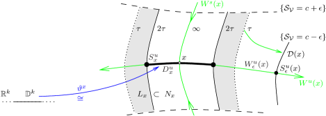
Figure 9: The $k$-disk $D^{u}_{x}\subset N_{x}$ and its bounding sphere $S^{u}_{x}\subset L_{x}$

Theorem 2.15 (Homology of Conley pairs).

Given a nondegenerate critical point $x$ of Morse index $k$ and one of the Conley pairs $(N_{x},L_{x})=(N_{x}^{{\varepsilon},\tau},L_{x}^{{\varepsilon},\tau})$ provided by Theorem 1.7. Fix a diffeomorphism

$$\vartheta^{x}:{\mathbb{D}}^{k}\to D^{u}_{x}:=\varphi_{-2\tau}\overline{W^{u}_{\varepsilon}(x)}$$ (36)

between the closed unit disk ${\mathbb{D}}^{k}\subset{\mathbb{R}}^{k}$ and the disk $D^{u}_{x}$ which is contained in $N_{x}\cap W^{u}(x)$ and whose boundary is given by $S^{u}_{x}:={\partial}D^{u}_{x}=\varphi_{-2\tau}S^{u}_{\varepsilon}(x)$ and lies in the exit set $L_{x}$; see Figure 9. Then there are the isomorphisms

(37)

which are non-trivial only in degree $k={\rm ind}_{\mathcal{V}}(x)$ and where $\iota$ denotes inclusion. Furthermore, it holds that $(\iota\circ\vartheta^{x})_{*}:[{\mathbb{D}}^{k}]\mapsto[D^{u}_{x}]\mapsto[D^{u}_{x}]$.

Proof.

Since $\vartheta^{x}:{\mathbb{D}}^{k}\to D^{u}_{x}$ is a diffeomorphism which maps ${\partial}{\mathbb{D}}^{k}$ to $S^{u}_{x}$ it induces an isomorphism on relative homology. Thus the image $D^{u}_{x}$ of the relative cycle ${\mathbb{D}}^{k}$ represents one of two generators of ${\rm H}_{*}(D^{u}_{x},S^{u}_{x})\cong{\mathbb{Z}}$. To distinguish them one needs to specify an orientation of $D^{u}_{x}$; see Definition 2.16. By (22) the boundary $S^{u}_{x}$ of $D^{u}_{x}$ is $\varphi_{-2\tau}S^{u}_{\varepsilon}(x)$ and it lies in $L_{x}$ by Proposition 2.13. Hence the inclusion $\iota:(D^{u}_{x},S^{u}_{x})\hookrightarrow(N_{x},L_{x})$ provides an element of ${\rm H}_{k}(N_{x},L_{x})$ denoted by $\iota_{*}[D^{u}_{x}]=[\iota(D^{u}_{x})]$ or simply by $[D^{u}_{x}]$. To see that $\iota_{*}[D^{u}_{x}]$ is actually a basis – in other words, that the inclusion $\iota$ induces an isomorphism – recall that $(N^{u}_{x},L_{x}^{u})=(N_{x}\cap W^{u}(x),L_{x}\cap W^{u}(x))$ and consider the homomorphisms

(38)

Here $\theta:=\theta^{\infty}:N_{x}\to N^{u}_{x}$ is the strong deformation retraction (27) referred to by Theorem D and $r=h_{1}:N^{u}_{x}\to D^{u}_{x}$ is the strong deformation retraction to be defined below. Because both deformation retractions are strong, we get that $r_{*}\theta_{*}\iota_{*}[D^{u}_{x}]=[id(id(\iota(D^{u}_{x}))]=[D^{u}_{x}]$. But $[D^{u}_{x}]$ generates ${\rm H}_{*}(D^{u}_{x},S^{u}_{x})$ and so $\iota_{*}$ has to be injective. Moreover, since isomorphisms map bases to bases and ${\theta_{*}}^{-1}{r_{*}}^{-1}([D^{u}_{x}])=\iota_{*}[D^{u}_{x}]$ it follows that $\iota_{*}$ is surjective, thus an isomorphism.

It remains to construct a map $h:[0,1]\times N^{u}_{x}\to N^{u}_{x}$, $(\lambda,\gamma)\mapsto h_{\lambda}(\gamma)$, providing a homotopy between $h_{0}=id_{N^{u}_{x}}$ and $r:=h_{1}:N^{u}_{x}\to D^{u}_{x}$ and such that $h_{\lambda}|_{D^{u}_{x}}=id_{D^{u}_{x}}$ for every $\lambda\in[0,1]$. Consider the annuli $X\supset A$ given by

$$X:=W^{u}(x)\setminus{\rm int\,}D^{u}_{x}=W^{u}(x)\setminus\varphi_{-2\tau}W^{u}_{\varepsilon}(x),\qquad A:=W^{u}(x)\setminus W^{u}_{\varepsilon}(x),$$

and the entrance time function ${\mathcal{T}}_{A}:X\mapsto[0,2\tau]$ as defined by (54) below while constructing the third isomorphism in the proof of Theorem B. By arguments analogous to the ones used during that construction ${\mathcal{T}}_{A}$ is lower semi-continuous by closedness of $A\subset X$ and upper semi-continuous by (forward) semi-flow invariance of $A$ in $X$. Then the map defined by

$$h_{\lambda}(\gamma):=\begin{cases}\gamma&\text{, $\gamma\in D^{u}_{x}$,}\\ \varphi_{\lambda({\mathcal{T}}_{A}(\gamma)-2\tau)}\gamma&\text{, $\gamma\in N^{u}_{x}\setminus{\rm int\,}D^{u}_{x}$,}\end{cases}$$

has all the desired properties. It is well defined since ${\mathcal{T}}_{A}$ vanishes on ${\partial}D^{u}_{x}$. ∎

Definition 2.16.

(i) In the setting of Theorem 2.15 assume ${\mathbb{D}}^{k}$ carries the canonical orientation. Pick an orientation $\langle x\rangle$ of $W^{u}(x)$. Then

$$\sigma_{\langle x\rangle}:=\begin{cases}+1&\text{, if $\vartheta^{x}:{\mathbb{D}}^{k}\to W^{u}(x)$ preserves orientation,}\\ -1&\text{, otherwise.}\end{cases}$$ (39)

is called the sign of $\vartheta^{x}$ with respect to $\langle x\rangle$.

(ii) Consider the linear transformation $\mu:={\rm diag}(-1,1,\dots,1)\in{\mathbb{R}}^{k\times k}$. It is an orientation reversing diffeomorphism of ${\mathbb{R}}^{k}$ and of ${\mathbb{D}}^{k}$. With the conventions

$$\mu^{0}={{\mathchoice{\rm 1\mskip-4.0mul}{\rm 1\mskip-4.0mul}{\rm 1\mskip-4.5mul}{\rm 1\mskip-5.0mul}}},\qquad\kappa_{\langle x\rangle}=\tfrac{1}{2}\left(1+\sigma_{\langle x\rangle}\right)\in\{0,1\}$$ (40)

we get the identity of induced isomorphisms

$$\begin{split}\sigma_{\langle x\rangle}\vartheta^{x}_{*}=(\vartheta^{x}\circ\mu^{\kappa_{\langle x\rangle}})_{k}:{\rm H}_{*}({\mathbb{D}}^{k},\SS^{k-1})\to{\rm H}_{k}\bigl{(}D^{u}_{x},S^{u}_{x}\bigr{)}\end{split}$$ (41)

which map the positive generator $a_{k}=[{\mathbb{D}}^{k}_{\langle\mathrm{can}\rangle}]$ is to the generator $[D^{u}_{\langle x\rangle}]$ of ${\rm H}_{k}\bigl{(}D^{u}_{x},S^{u}_{x}\bigr{)}\cong{\mathbb{Z}}$. Here $D^{u}_{\langle x\rangle}$ denotes the relative cycle $D^{u}_{x}$ oriented by $\langle x\rangle$.

3 Morse filtration and natural isomorphism

In section 3 we construct the natural isomorphism in Theorem A, in other words, we calculate singular homology of the sublevel set $\Lambda^{a}M$ in terms of the homology of the Morse complex $\left({\rm CM}^{a}_{*}(V),{\partial}^{M}_{*}(V,v_{a})\right)$ defined in section 1.1. Recall that the chain group ${\rm CM}^{a}_{*}(V)$ is the free Abelian group generated by oriented critical points $\langle x\rangle\in{\rm Crit}^{a}$ of the Morse function ${\mathcal{S}}_{V}$ – without assigning the role of a distinct generator to one of the two possible orientations since we divide out subsequently by the relation (3). The Morse boundary operator counts heat flow trajectories $u$ between critical points of Morse index difference one according to how the corresponding push-forward orientations $u_{*}\langle x\rangle$ match at the lower end.

The key idea is to consider an intermediate chain complex associated to a cellular filtration which, on the level of homology, is already known to be naturally isomorphic to singular homology. On the other hand, the additional geometric data provided by the Morse-Smale function ${\mathcal{S}}_{\mathcal{V}}$ given by (5) gives rise to a very particular filtration, namely, a Morse filtration whose associated cellular chain complex equals the Morse complex up to natural identification. In the case of a finite dimensional manifold this idea has been used by Milnor [9] in the context of a self-indexing Morse function $f:M\to{\mathbb{R}}$ in which case just the sublevel sets $F_{k}:=f^{-1}((-\infty,k+\tfrac{1}{2}])$ itself provide a Morse filtration. For a Banach manifold with a genuine flow generated by a $C^{1}$ vector field a suitable filtration has been constructed by Abbondandolo and Majer [1] who, moreover, provide full details of their construction of an isomorphism (depending on choices of orientations) between Morse and singular homology.

Obviously the Hilbert manifold of $W^{1,2}$ loops in $M$ is the natural domain of the action functional ${\mathcal{S}}_{\mathcal{V}}$ and its Hilbert manifold structure facilitates the analysis. Moreover, the space $\Lambda^{a}M$ of $W^{1,2}$ loops in $M$ whose action is less or equal than $a$ is homotopy equivalent to its subset ${\mathcal{L}}^{a}M$ of smooth loops (see e.g. [8, § 17] or footnote). Thus singular homology of both spaces is naturally isomorphic and Theorem A covers [17, Thm. A.7]. Furthermore, it is not necessary that the potential ${\mathcal{V}}$ is a sum (4) of a geometric potential $V$ and an abstract perturbation $v_{a}$. All we need is that ${\mathcal{V}}$ satisfies axioms (V0)–(V3) in [28] and is Morse-Smale below the regular level $a$ in the functional analytic sense of [28, §1]. Any ${\mathcal{V}}$ that satisfies (V0)–(V3) gives rise to a $C^{1}$ semi-flow

$$\varphi:(0,\infty)\times\Lambda^{a}M\to\Lambda^{a}M,\qquad\Lambda^{a}M:=\{{\mathcal{S}}_{\mathcal{V}}\leq a\},$$ (42)

which extends continuously to zero; see e.g. [27].

In what follows we construct the natural isomorphism for the semi-flow (42). For simplicity think of ${\mathcal{V}}$ as given by (4). To avoid overusing the word ’continuous’ all maps are assumed to be continuous unless specified differently.

3.1 Morse filtration

Assume ${\mathcal{V}}$ is a perturbation that satisfies axioms (V0)–(V3) in [28] and ${\mathcal{S}}_{\mathcal{V}}$ is Morse-Smale below the regular level $a$. We construct a Morse filtration ${\mathcal{F}}=\left(F_{k}\right)$ associated to ${\mathcal{S}}_{\mathcal{V}}:\Lambda^{a}M\to{\mathbb{R}}$ such that, in addition, each set $F_{k}$ is open and semi-flow invariant.

Consider the closed ball $B_{x}^{\rho}$ of radius $\rho>0$ about $x$ with respect to the $W^{1,2}$ metric on $\Lambda M$. Since $a$ is a regular value and the critical points are nondegenerate there is a sufficiently small radius $\rho=\rho(a)>0$ such that

$$B_{x}^{\rho}\subset\Lambda^{a}M,\qquad B_{x}^{\rho}\cap B_{y}^{\rho}=\emptyset,$$ (43)

for any two distinct elements $x$ and $y$ of the finite set ${\rm Crit}^{a}$. The Morse-Smale condition guarantees that there are no flow lines from one critical point to another one of equal or larger Morse index. The following lemma generalizes this principle, firstly, to small neighborhoods (cf. [1, Lemma 2.5]) and, secondly, to semi-flows. More precisely, the lemma guarantees that the Morse index strictly decreases whenever there is a flow trajectory from $B_{x}^{\rho}$ to $B_{y}^{\rho}$ and $\rho>0$ is sufficiently small. We postpone proofs.

Lemma 3.1 (Morse-Smale on neighborhoods).

There is a constant $\rho=\rho(a)>0$ such that the pre-images ${\varphi_{s}}^{-1}B_{y}^{\rho}$ satisfy

$$B_{x}^{\rho}\cap{\varphi_{s}}^{-1}B_{y}^{\rho}=\emptyset,\quad\forall s\geq 0,$$ (44)

for all pairs of distinct critical points $x,y\in{\rm Crit}^{a}$ with ${\rm ind}_{\mathcal{V}}(x)\leq{\rm ind}_{\mathcal{V}}(y)$.

Hypothesis 3.2.

Assume the perturbation ${\mathcal{V}}$ satisfies (V0)–(V3) in [28] and the Morse-Smale condition holds below the regular level $a$ of ${\mathcal{S}}_{\mathcal{V}}$.

1. Fix a constant $\rho=\rho(a)>0$ sufficiently small such that (43) and (44) hold true and such that for each critical point $x\in{\rm Crit}^{a}$ the local coordinate chart $(\Phi,\Phi(B^{u}\times B^{+}))$ about $x\in\Lambda M$ covers the ball $B_{x}^{2\rho}$. Here $B^{u}\times B^{+}\subset X^{-}\oplus X^{+}$ is a product of balls contained in ${\mathcal{B}}_{\rho_{0}}$ with $B^{u}\subset W^{u}$; see Hypothesis 2.2 (H1). Pick constants ${\varepsilon}>0$ sufficiently small and $\tau>0$ sufficiently large such that for each $x\in{\rm Crit}^{a}$ Theorem C (Invariant stable foliation) and Theorem 1.7 (Conley pair) hold true. In particular, every $x\in{\rm Crit}^{a}$ admits a Conley pair, namely $(N_{x},L_{x})=(N_{x}^{{\varepsilon},\tau},L_{x}^{{\varepsilon},\tau})$ defined by (15) and (16). By Theorem C part d) we assume that $N_{x}\subset B_{x}^{\rho}$. Consequently $N_{x}\cap N_{y}=\emptyset$ whenever $x\not=y$.

From now on we assume Hypothesis 3.2 and use the notation

$$N_{k}:=\bigcup_{x\in{\rm Crit}^{a}_{k}}N_{x},\qquad L_{k}:=\bigcup_{x\in{\rm Crit}^{a}_{k}}L_{x},\qquad k\in{\mathbb{Z}}.$$ (45)

By definition a union over the empty set is the empty set. Since $N_{x}\subset B_{x}^{\rho}$ both unions are unions of disjoint sets by (43). We denote the maximal Morse index among the critical points below level $a$ by

$$m=m(a):=\max_{x\in{\rm Crit}^{a}}{\rm ind}_{\mathcal{V}}(x).$$ (46)

Observe that ${\rm Crit}_{0}^{a}\not=\emptyset$ since the action ${\mathcal{S}}_{\mathcal{V}}$ is bounded below. For such a critical point $x$ of Morse index $0$ the Conley index pair $(N_{x},L_{x})$ consists of the ascending disk $N_{x}=N_{x}(x)=W^{s}_{\varepsilon}(x)$ by Theorem C part a) and the empty exit set $L_{x}=\emptyset$. Note that the ascending disk $W^{s}_{\varepsilon}(x):=W^{s}(x)\cap\{{\mathcal{S}}_{\mathcal{V}}<{\mathcal{S}}_{\mathcal{V}}(x)+{\varepsilon}\}$ is open and semi-flow invariant. Hence $N_{0}$ is a finite union of (open and semi-flow invariant) disjoint ascending disks and $L_{0}=\emptyset$. Next observe that for each $T>0$ the set $F_{0}=F_{0}(T):={\varphi_{T}}^{-1}N_{0}$ is semi-flow invariant. By continuity of $\varphi_{T}$ it is also open. Assume $k>0$ is the next larger realized Morse index, that is $k$ is the minimal Morse index among the elements of ${\rm Crit}^{a}\setminus{\rm Crit}^{a}_{0}$. Consider the unstable manifold of a critical point $x_{k}$ of Morse index $k$. Each element $\gamma\not=x_{k}$ moves in finite time $T_{\gamma}$ into the neighborhood $N_{0}$ of ${\rm Crit}_{0}$ by existence of the asymptotic forward limit [27, Thm. 9.14]. The Morse-Smale condition guarantees that the Morse index of the asymptotic forward limit is strictly less than $k$, thus indeed zero by minimality of $k$. Hence $\gamma\in{\varphi_{T_{\gamma}}}^{-1}N_{0}$. In fact, a much stronger statement is true: There is a time $T_{k}>0$ such that the pre-image ${\varphi_{T_{k}}}^{-1}N_{0}$ contains all elements $\gamma$ of the infinite dimensional exit set $L_{k}$ of $N_{k}$.

Proposition 3.3 (Uniform time).

Given Hypothesis 3.2, suppose $A$ is an open semi-flow invariant subset of $\Lambda^{a}M$ containing all critical points of Morse index less or equal to $k$ and no others. In the case $k<m(a)$ there is a time $T_{k+1}\geq 0$ such that $L_{k+1}\subset{\varphi_{T_{k+1}}}^{-1}A$. If $L_{k+1}=\emptyset$, set $T_{k+1}:=0$. In the case $k=m(a)$ of maximal Morse index there is a time $T_{m+1}\geq 0$ such that $\Lambda^{a}M={\varphi_{T_{m+1}}}^{-1}A$.

Definition of the Morse filtration

The first step in the construction of the Morse filtration ${\mathcal{F}}=\left(F_{k}\right)_{k\in{\mathbb{Z}}}$ associated to ${\mathcal{S}}_{\mathcal{V}}:\Lambda^{a}M\to{\mathbb{R}}$ is to set $F_{k}:=\emptyset$ whenever $k<0$. Now consider the time $T_{1}$ given by Proposition 3.3 for $A=N_{0}$. It provides the crucial inclusion

$$L_{1}\subset{\varphi_{T_{1}}}^{-1}N_{0}=:F_{0}$$

illustrated by Figure 10.

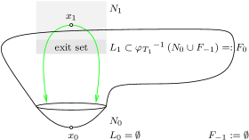
Figure 10: Morse filtration ${\mathcal{F}}=\left(\emptyset\subset F_{0}\subset F_{1}\subset\dots\subset F_{m}=\Lambda^{a}M\right)$

Because the exit set $L_{1}$ of $N_{1}$ is contained in the semi-flow invariant set $F_{0}$, the union $N_{1}\cup F_{0}$ is semi-flow invariant as well. Trivially it is also open. Next consider the time $T_{2}$ provided by Proposition 3.3 for $A=N_{1}\cup F_{0}$. Hence

$$L_{2}\subset{\varphi_{T_{2}}}^{-1}\left(N_{1}\cup F_{0}\right)=:F_{1}$$

and $F_{1}$ is open and semi-flow invariant by the same reasoning as above. Note that if there are no critical points of Morse index $1$, then $F_{1}={\varphi_{0}}^{-1}(\emptyset\cup F_{0})=F_{0}$. Proceeding iteratively we obtain a sequence of open semi-flow invariant subsets

$$\emptyset=F_{-1}\subset F_{0}\subset F_{1}\subset\ldots\subset F_{m}=\Lambda^{a}M.$$

More precisely, recalling that $\varphi_{T}:\Lambda^{a}M\to\Lambda^{a}M$ for any $T\geq 0$ we set

$$F_{k}:={\varphi_{T_{k+1}}}^{-1}\left(N_{k}\cup F_{k-1}\right)\supset L_{k+1},\qquad k=0,\ldots,m-1,$$ (47)

and

$$F_{m}:={\varphi_{T_{m+1}}}^{-1}\left(N_{m}\cup F_{m-1}\right)=\Lambda^{a}M.$$ (48)

Here $T_{k+1}$ is the time associated by Proposition 3.3 to the set $A=N_{k}\cup F_{k-1}$. Note that if there are no critical points whose Morse index is $k$ or $k+1$, then $F_{k}=F_{k-1}$ and $F_{k+1}={\varphi_{T_{k+2}}}^{-1}(F_{k-1})$. Set $F_{\ell}:=\Lambda^{a}M$ whenever $\ell>m$.

Proofs

The proof of Theorem B uses Proposition 3.3 (Uniform time) which relies on Lemma 3.1 (Morse-Smale on neighborhoods). So we start with the

Proof of Lemma 3.1 (Morse-Smale on neighborhoods).

Assume the lemma is not true. Then there are critical points $x\not=y$ below level $a$ with ${\rm ind}_{\mathcal{V}}(x)\leq{\rm ind}_{\mathcal{V}}(y)$, sequences of constants $\rho_{\nu}\searrow 0$ and $s_{\nu}\geq 0$, and a sequence of loops $\gamma^{\nu}\in B_{x}^{\rho_{\nu}}$ such that $\varphi_{s_{\nu}}\gamma^{\nu}\in B_{y}^{\rho_{\nu}}$. Thus $\gamma^{\nu}$ converges to $x$ and $\varphi_{s_{\nu}}\gamma^{\nu}$ to $y$ in the $W^{1,2}$ topology, as $\nu\to\infty$. Moreover, it follows that $s_{\nu}\to\infty$, as $\nu\to\infty$. To see the latter assume by contradiction that the sequence $s_{\nu}$ is bounded. Then there is a subsequence, still denoted by $s_{\nu}$, such that $s_{\nu}$ converges to a constant $T\geq 0$. By continuity of the semi-flow $\varphi$ we conclude that $\varphi_{s_{\nu}}\gamma^{\nu}$ converges in $W^{1,2}$ to $\varphi_{T}x$, as $\nu\to\infty$. But $\varphi_{T}x=x$ since critical points are fixed points. Since $\varphi_{s_{\nu}}\gamma^{\nu}$ converges also to $y$ in $W^{1,2}$ we obtain the contradiction $x=y$.

Now consider the sequence of heat flow trajectories $u^{\nu}:[0,s_{\nu}]\times S^{1}\to M$,

$$u^{\nu}(s,t):=\left(\varphi_{s}\gamma^{\nu}\right)(t).$$

Since the action is nonincreasing along heat flow trajectories and since $\gamma^{\nu}\in B_{x}^{\rho_{\nu}}\subset\Lambda^{a}M$ it follows that

$$\max_{s\in[0,s_{\nu}]}{\mathcal{S}}_{\mathcal{V}}\left(u^{\nu}(s,\cdot)\right)\leq{\mathcal{S}}_{\mathcal{V}}\left(\gamma^{\nu}\right)\leq a.$$

So we have a uniform action bound on compact subcylinders of $[0,\infty)\times S^{1}$ for the sequence $u^{\nu}$ of heat flow trajectories. By the arguments used to prove [28, Prop. 3] (Convergence on compact sets) and [28, Le. 4] (Compactness up to broken trajectories) we obtain critical points $x=x_{0},\dots,x_{\ell}=y$, where $\ell\geq 1$, and for each $k\in\{1,\ldots,\ell\}$ a connecting trajectory $u_{k}\in{\mathcal{M}}(x_{k-1},x_{k};{\mathcal{V}})$ with ${\partial}_{s}u_{k}\not\equiv 0$. By the Morse-Smale condition the Morse index of $x_{k}$ is strictly smaller than the Morse index of $x_{k-1}$. Thus ${\rm ind}_{\mathcal{V}}(x_{0})>{\rm ind}_{\mathcal{V}}(x_{m})$. Contradiction. ∎

Remark 3.4.

The action functional ${\mathcal{S}}_{\mathcal{V}}:\Lambda M\to{\mathbb{R}}$, $\gamma\mapsto\frac{1}{2}\mathopen{\|}\dot{\gamma}\mathclose{\|}_{2}^{2}-{\mathcal{V}}(\gamma)$, is continuously differentiable. To see this observe that

$$d{\mathcal{S}}_{\mathcal{V}}(\gamma)\xi=\langle\dot{\gamma},\nabla\kern-2.15277pt{}_{t}\xi\rangle_{L^{2}}-\langle{\rm grad}{\mathcal{V}}(\gamma),\xi\rangle_{L^{2}}$$

for all $\gamma\in\Lambda M$ and $\xi\in W^{1,2}(S^{1},\gamma^{*}TM)$. Continuity of the first term is obvious and for the second term it follows from axioms (V0)–(V1). By definition the $L^{2}$-gradient of ${\mathcal{S}}_{\mathcal{V}}$ is determined by the identity $d{\mathcal{S}}_{\mathcal{V}}(\gamma)\xi=\langle{\rm grad}{\mathcal{S}}_{\mathcal{V}}(\gamma),\xi\rangle_{L^{2}}$ for all $\gamma\in\Lambda M$ and $\xi\in W^{1,2}(S^{1},\gamma^{*}TM)$. If $\gamma$ is of higher regularity $W^{2,2}$, then we can carry out integration by parts and ${\rm grad}{\mathcal{S}}_{\mathcal{V}}$ becomes a continuous section of the Hilbert space bundle over $W^{2,2}(S^{1},M)$ whose fiber over $\gamma$ is given by the Hilbert space $L^{2}(S^{1},\gamma^{*}TM)$ of $L^{2}$ vector fields along $\gamma$. In this case we obtain the explicit representation

$${\rm grad}{\mathcal{S}}_{\mathcal{V}}(\gamma)=-\nabla\kern-2.15277pt{}_{t}{\partial}_{t}\gamma-{\rm grad}{\mathcal{V}}(\gamma)$$

whenever $\gamma\in W^{2,2}(S^{1},\gamma^{*}TM)$.

Proof of Proposition 3.3 (Uniform time)..

Key ingredients will be Palais-Smale, Morse-Smale on neighborhoods, and the fact that the action functional ${\mathcal{S}}_{\mathcal{V}}$ is bounded from below. Recall Hypothesis 3.2 on the choices of ${\mathcal{V}}$, $\rho$, ${\varepsilon}$, and $\tau$.

Fix $k<m(a)$ and pick an open semi-flow invariant subset $A\subset\Lambda^{a}M$ which contains ${\rm Crit}^{a}_{\leq k}$ but no other critical points. Assume $L_{k+1}\not=\emptyset$, otherwise we are done by setting $T_{k+1}=0$. Now assume by contradiction that there is no time $T\geq 0$ such that $\varphi_{T}L_{k+1}\subset A$. In this case there are sequences of positive reals $s_{\nu}\to\infty$ and of elements $\gamma^{\nu}$ of $L_{k+1}$ such that $\varphi_{s_{\nu}}\gamma^{\nu}\notin A$ for every $\nu\in{\mathbb{N}}$. Choosing subsequences, still denoted by $s_{\nu}$ and $\gamma^{\nu}$, we may assume that all $\gamma^{\nu}$ lie in the same path connected component $L_{x}$ of $L_{k+1}$ for some $x\in{\rm Crit}^{a}_{k+1}$. Here we use that ${\rm Crit}^{a}_{k+1}$ is a finite set since ${\mathcal{S}}_{\mathcal{V}}$ is Morse below level $a$; see [26].

Now consider the open neighborhood of ${\rm Crit}^{a}$ in $\Lambda^{a}M$ defined by

$$U:=A\cup\left(N_{x}\setminus L_{x}\right)\cup\bigcup_{y\in{\rm Crit}^{a}_{\geq k+1}\setminus\{x\}}N_{y}.$$

Indeed $A$ is open by assumption and so are the neighborhoods $N_{x}$ and $N_{x}\setminus L_{x}$ of $x$ by Theorem 1.7 and Definition 1.6 of a Conley pair. Note that

$$\kappa:=\inf_{\gamma\in\Lambda^{a}M\setminus U}\left\|{\rm grad}{\mathcal{S}}_{\mathcal{V}}(\gamma)\right\|_{2}>0$$

is strictly positive. To see this assume by contradiction that $\kappa=0$. Then there is a sequence $z^{i}$ in $\Lambda^{a}M\setminus U$ such that $\mathopen{\|}{\rm grad}{\mathcal{S}}_{\mathcal{V}}(z^{i})\mathclose{\|}_{2}\to 0$, as $i\to\infty$. So by Palais-Smale a subsequence converges to some critical point in the closed set $\Lambda^{a}M\setminus U$. But all critical points below level $a$ lie in the open set $U$. Contradiction.

None of the elements $\varphi_{s_{\nu}}\gamma^{\nu}$ of $\Lambda^{a}M$ lies in $U$: Indeed $\varphi_{s_{\nu}}\gamma^{\nu}\notin A$ by assumption. Furthermore, such an element cannot lie in the union of the $N_{y}$’s, because otherwise we would have a flow line from $N_{x}\subset B_{x}^{\rho}$ to $N_{y}\subset B_{y}^{\rho}$ thereby contradicting Lemma 3.1 (Morse-Smale on neighborhoods) since ${\rm ind}_{\mathcal{V}}(x)\leq{\rm ind}_{\mathcal{V}}(y)$. It remains to check that $\varphi_{s_{\nu}}\gamma^{\nu}\notin N_{x}\setminus L_{x}$. To see this set $c:={\mathcal{S}}_{\mathcal{V}}(x)$ and recall that $\gamma^{\nu}$ lies in $L_{x}$ which is positively invariant in $N_{x}$ by Definition 1.6 (iii). Assume that the semi-flow trajectory through $\gamma^{\nu}$ leaves $L_{x}$, thus simultaneously $N_{x}$, say at a time $s_{*}$. (Otherwise, if it stayed inside $L_{x}$ forever, we are done.) By definition of $N_{x}=N_{x}^{{\varepsilon},\tau}$ and the downward gradient property the point $\varphi_{s_{*}}\gamma^{\nu}$ reaches the action level $c-{\varepsilon}$ precisely after time $\tau$, that is ${\mathcal{S}}_{\mathcal{V}}(\varphi_{\tau}(\varphi_{s_{*}}\gamma^{\nu}))=c-{\varepsilon}$. Since the action decreases along heat flow trajectories we conclude that ${\mathcal{S}}_{\mathcal{V}}(\varphi_{\tau}(\varphi_{s_{*}+s}\gamma^{\nu}))\leq c-{\varepsilon}$ whenever $s\geq 0$. Thus the semi-flow line through $\varphi_{s_{*}}\gamma^{\nu}$ cannot re-enter $N_{x}$ (nor its subset $L_{x}$). To summarize we know that $\varphi_{[0,s_{*})}\gamma^{\nu}\subset L_{x}$ and $\varphi_{[s_{*},\infty)}\gamma^{\nu}\cap N_{x}=\emptyset$. But this proves that $\varphi_{[0,\infty)}\gamma^{\nu}\cap\left(N_{x}\setminus L_{x}\right)=\emptyset$.

More generally, it even holds that $\varphi_{s}\gamma^{\nu}\notin U$ whenever $s\in[0,s_{\nu}]$ and $\nu\in{\mathbb{N}}$: Indeed $\varphi_{s}\gamma^{\nu}$ cannot lie in $A$, since $A$ is semi-flow invariant by assumption and $\varphi_{s_{\nu}}\gamma^{\nu}\notin A$. That $\varphi_{s}\gamma^{\nu}\notin N_{x}\setminus L_{x}$ has been proved in the previous paragraph. The statement for the union of the $N_{y}$’s follows by the same Morse-Smale argument given in the previous paragraph for $s=s_{\nu}$.

To finally derive a contradiction use the fact that $\varphi_{s}$ is the semi-flow generated by the negative $L^{2}$-gradient of ${\mathcal{S}}_{\mathcal{V}}$ to obtain that

$$\begin{split}{\mathcal{S}}_{\mathcal{V}}(\gamma^{\nu})-{\mathcal{S}}_{\mathcal{V}}(\varphi_{s_{\nu}}\gamma^{\nu})&=\int_{s_{\nu}}^{0}\frac{d}{ds}{\mathcal{S}}_{\mathcal{V}}(\varphi_{s}\gamma^{\nu})\,ds\\ &=\int_{s_{\nu}}^{0}d{\mathcal{S}}_{\mathcal{V}}|_{\varphi_{s}(\gamma^{\nu})}\circ\left(\frac{d}{ds}\varphi_{s}\gamma^{\nu}\right)ds\\ &=\int_{0}^{s_{\nu}}\left\|{\rm grad}{\mathcal{S}}_{\mathcal{V}}\left(\varphi_{s}\gamma^{\nu}\right)\right\|_{2}^{2}\,ds\\ &\geq\kappa^{2}s_{\nu}\end{split}$$

where the inequality uses the definition of $\kappa$ and the fact that $\varphi_{s}\gamma^{\nu}\notin U$ whenever $s\in[0,s_{\nu}]$. Since $\kappa>0$, we get that

$${\mathcal{S}}_{\mathcal{V}}(\varphi_{s_{\nu}}\gamma^{\nu})\leq{\mathcal{S}}_{\mathcal{V}}(\gamma^{\nu})-\kappa^{2}s_{\nu}\leq a-\kappa^{2}s_{\nu}\longrightarrow-\infty,\quad\text{as $\nu\to\infty$.}$$

But this contradicts the fact that ${\mathcal{S}}_{\mathcal{V}}$ is bounded from below by $-C_{0}$ where $C_{0}$ is the constant in axiom (V0). This concludes the proof of the case $k<m$.

In the case $k=m$ pick an open semi-flow invariant subset $A\subset\Lambda^{a}M$ which contains ${\rm Crit}^{a}$. Assume by contradiction that there is no time $T\geq 0$ such that $\varphi_{T}(\Lambda^{a}M)\subset A$. Then there are sequences $s_{\nu}\to\infty$ and $\gamma^{\nu}$ in $(\Lambda^{a}M)\setminus A$ such that $\varphi_{s_{\nu}}\gamma^{\nu}\notin A$ for $\nu\in{\mathbb{N}}$. Now repeat for the much simpler $U:=A$ the argument given in the case $k<m$. This proves Proposition 3.3. ∎

Proof of Theorem B (Morse filtration and chain group isomorphism).

First we pick an integer $k\in\{0,\ldots,m(a)\}$ where $m(a)$ is the maximal Morse index (46) among the (finitely many) elements of ${\rm Crit}^{a}$. Observe that a set $A$ is semi-flow invariant, that is $\varphi_{T}A\subset A$ for every time $T\geq 0$, if and only if $A\subset{\varphi_{T}}^{-1}(A)$ for every time $T\geq 0$. This observation for $A=N_{k}\cup F_{k-1}$ and the definition of $F_{k}$, see (47) and (48), show that

$$F_{k-1}\subset\left(N_{k}\cup F_{k-1}\right)\subset{\varphi_{T_{k+1}}}^{-1}\left(N_{k}\cup F_{k-1}\right)=:F_{k}.$$ (49)

This proves (i) in Definition 1.3 of a cellular filtration. Because $F_{m}=\Lambda^{a}M$ by (48), condition (ii) is obviously true. Thus to prove that ${\mathcal{F}}(\Lambda^{a}M)=(F_{k})$ is a cellular filtration of $\Lambda^{a}M$ it remains to verify condition (iii) in Definition 1.3.

Putting together the individual isomorphisms given by (37) for each critical point $x$ provides the isomomorphism

$$\begin{split}\Theta_{k}:{\rm CM}_{k}^{a}({\mathcal{S}}_{\mathcal{V}})&\to\bigoplus_{x\in{\rm Crit}^{a}_{k}}{\rm H}_{k}(N_{x},L_{x})\\ \langle x\rangle&\mapsto\Bigl{(}0,\dots,0,\underbrace{\left(\iota\circ\vartheta^{x}\right)_{*}(\sigma_{\langle x\rangle}a_{k})}_{\text{$=[D^{u}_{\langle x\rangle}]$ by~{}(\ref{eq:vartheta-or})}},0,\dots,0\Bigr{)}\end{split}$$

between abelian groups. It is well defined since $\sigma_{\langle x\rangle}\in\{\pm 1\}$ defined by (39) changes sign when replacing the orientation $\langle x\rangle$ of the unstable manifold of $x$ by the opposite orientation $-\langle x\rangle$.

By (49) and (47) there is the inclusion of pairs $\iota:(N_{k},L_{k})\hookrightarrow(F_{k},F_{k-1})$. Further below we will prove that it induces an isomorphism on homology

$$\iota_{*}:{\rm H}_{*}(N_{k},L_{k})\stackrel{{\scriptstyle\cong}}{{\longrightarrow}}{\rm H}_{*}(F_{k},F_{k-1}).$$ (50)

Recall from (45) that $N_{k}=\cup_{x}N_{x}$ is a union of disjoint subsets. Therefore

$$\oplus\iota^{x}_{*}:\bigoplus_{x\in{\rm Crit}^{a}_{k}}{\rm H}_{\ell}(N_{x},L_{x})\stackrel{{\scriptstyle\cong}}{{\longrightarrow}}{\rm H}_{\ell}(N_{k},L_{k})$$

is an isomorphism for each $\ell\in{\mathbb{Z}}$; see e.g. [4, III Proposition 4.12]. Now if $\ell\not=k$, then (each summand of) the left hand side is zero by Theorem 2.15. Hence ${\rm H}_{\ell}(F_{k},F_{k-1})=0$ by (50), that is condition (iii) in Definition 1.3 holds true, and ${\mathcal{F}}(\Lambda^{a}M)=(F_{k})$ is a cellular filtration of $\Lambda^{a}M$. If $\ell=k$, then again by Theorem 2.15 each group ${\rm H}_{k}(N_{x},L_{x})$ is generated by the homology class of the disk $D^{u}_{x}\subset W^{u}(x)$. By (50) this shows that ${\mathcal{F}}(\Lambda^{a}M)$ is a Morse filtration.

Next assume $b\leq a$ is also a regular value. It’s a first impulse to take as ${\mathcal{F}}(\Lambda^{b}M)=(F_{k}^{b})$ the sequence of intersections $(F_{k}\cap\Lambda^{b}M)$. But then how to calculate ${\rm H}_{\ell}(F_{k}\cap\Lambda^{b}M,F_{k-1}\cap\Lambda^{b}M)$? Let’s start differently with the simple observations that ${\rm Crit}^{b}\subset{\rm Crit}^{a}$ and that the sets $N_{k}$ and $L_{k}$ defined by $($45$)_{a}$ contain, respectively, the sets $N_{k}^{b}$ and $L_{k}^{b}$ given by $($45$)_{b}$. Now define the sets

$${\mathcal{F}}(\Lambda^{b}M)=\left(F_{k}^{b}\right)$$ (51)

iteratively by $($47$)_{b}$ using the sets $N_{k}^{b}$ and $F_{k-1}^{b}$ and taking pre-images with respect to the semi-flow on $\Lambda^{b}M$. However, concerning the new times $T_{k+1}^{b}$ observe that setting $T_{k+1}^{b}$ equal to the old time $T_{k+1}=T_{k+1}(a)$ is absolutely fine to satisfy the crucial condition $F_{k}^{b}\supset L_{k+1}^{b}$. The proof that ${\mathcal{F}}(\Lambda^{b}M)$ defined this way is a Morse filtration is no different from the proof for ${\mathcal{F}}(\Lambda^{a}M)$.

To complete the proof it remains to establish the isomorphism (50). Similarly as in (38) the idea is to establish a number of consecutive isomorphisms

$$\begin{split}{\rm H}_{\ell}(F_{k},F_{k-1})&\stackrel{{\scriptstyle 1}}{{\cong}}{\rm H}_{\ell}(N_{k}\cup F_{k-1},F_{k-1})\\ &\stackrel{{\scriptstyle 2}}{{\cong}}{\rm H}_{\ell}(N_{k},N_{k}\cap F_{k-1})\\ &\stackrel{{\scriptstyle 3}}{{\cong}}{\rm H}_{\ell}(N_{k},L_{k})\end{split}$$ (52)

and show that each generator $[D^{u}_{x}]$ is invariant under the composition of these isomorphisms. So the image under $\iota_{*}$ of any basis of ${\rm H}_{*}(N_{k},L_{k})$ consisting of such elements $[D^{u}_{x}]$, one for each $x\in{\rm Crit}^{a}_{k}$, is an isomorphic image of that same basis. Hence $\iota_{*}$ takes bases in bases and therefore it is an isomorphism; cf. (38).

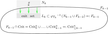
Figure 11: The sets $L_{k}\subset N_{k}$ and $F_{k-1}$

The first isomorphism uses the fact that the open semi-flow invariant sets

$$X:=F_{k}:={\varphi_{T_{k+1}}}^{-1}(N_{k}\cup F_{k-1}),\qquad A:=N_{k}\cup F_{k-1},$$

are homotopy equivalent: Reciprocal homotopy equivalences are given by

$$r:X\to A,\;\gamma\mapsto\varphi_{T_{k+1}}\gamma,\qquad\iota:A\hookrightarrow X={\varphi_{T_{k+1}}}^{-1}(A),$$ (53)

where $\iota$ denotes inclusion. Indeed $\iota\circ r$ is homotopic to $id_{X}$ via the homotopy $\{h_{\lambda}:X\to X,\gamma\mapsto\varphi_{\lambda T_{k+1}}\gamma\}_{\lambda\in[0,1]}$ and $r\circ\iota$ is homotopic to $id_{A}$ via the homotopy $\{f_{\lambda}:A\to A,\gamma\mapsto\varphi_{\lambda T_{k+1}}\gamma\}_{\lambda\in[0,1]}$. Now by homotopy equivalence of the sets $X$ and $A$ their singular homology groups are isomorphic; see e.g. Corollary 5.3 in [4, III]. Hence $\mathrm{H}_{*}(X,A)=0$ by the homology sequence of the pair $(X,A)$, see loc. cit. (3.2), and this implies the first isomorphism (use the homology sequence of the triple $B\subset A\subset X$ for $B=F_{k-1}$; loc. cit. (3.4)).

Alternatively, observe that $\iota$ and $r$ are reciprocal homotopy equivalences as maps of pairs $r:(X,B)\to(A,B)$ and $\iota:(A,B)\to(X,B)$ since both homotopies $h_{\lambda}$ and $f_{\lambda}$ preserve the semi-flow invariant set $B=F_{k-1}$. Thus the induced map on homology $r_{*}:{\rm H}_{*}(X,B)\to{\rm H}_{*}(A,B)$ is an isomorphism with inverse $\iota_{*}$; see e.g. Corollary 5.3 in [4, Chapter III].

Since $r=\varphi_{T_{k+1}}$ leaves the parts ${\rm int\,}D^{u}_{x}$ of the disks $D^{u}_{x}$ outside $L_{k}$ invariant (as sets) it holds that $[r(D^{u}_{x})]=[D^{u}_{x}]$ as elements of ${\rm H}_{*}(N_{k},L_{k})$.

The second isomorphism uses the excision axiom. Consider the topological space $X:=N_{k}\cup F_{k-1}$ and its subset $A:=F_{k-1}$ which is open in $X$ by openness of $F_{k-1}$ in $\Lambda^{a}M$. For the same reason $N_{k}$ is open in $X$. Therefore $N_{k}\cap F_{k-1}$ is open in $X$. Observe that

$$X=N_{k}\setminus(N_{k}\cap F_{k-1})\cup(N_{k}\cap F_{k-1})\cup F_{k-1}\setminus(N_{k}\cap F_{k-1})$$

is a union of three disjoint sets of which the second one is open. Thus the complement of set two is closed and consists of the disjoint sets one and three. Hence each of them is closed in $X$. Note that set three is equal to $B:=F_{k-1}\setminus N_{k}$. Since ${\rm cl\,}B=B\subset A={\rm int\,}A$ we are in position to apply the excision axiom in order to cut off $B$ from $X$ and from $A$ without changing relative homology; see Figure 11. and e.g. Corollary 7.4 in [4, III].

Note that all disks $D^{u}_{x}$ are disjoint from the cut off set $B$. Therefore excision does not affect any of these disks.

The third isomorphism is based on the fact that there is a strong deformation retraction $r:A:=N_{k}\cap F_{k-1}\to L_{k}=:B$ as illustrated by Figure 11. Hence the singular homology groups of $A$ and $B$ are isomorphic; see e.g. Corollary 5.3 in [4, III]. Thus $\mathrm{H}_{*}(A,B)=0$ by the homology sequence of the pair $(A,B)$, see loc. cit. (3.2), which implies existence of the third isomorphism ${\rm H}_{*}(N_{k},A)\cong{\rm H}_{*}(N_{k},B)$ in (52) – to see this use the homology sequence of the triple $B\subset A\subset N_{k}$; see loc. cit. (3.4). Because $r$ is defined (below) by flowing points forward until $L_{k}$ is reached, the disks $D^{u}_{x}\subset W^{u}(x)$ are invariant (as sets) under $r$ and therefore $[r(D^{u}_{x})]=[D^{u}_{x}]$ as elements of ${\rm H}_{*}(N_{k},L_{k})$.

To construct the strong deformation retraction $r:A\to B$ consider the entrance time function

$$\begin{split}{\mathcal{T}}={\mathcal{T}}_{L_{k}}:N_{k}\cap F_{k-1}&\to[0,\infty)\\ \gamma&\mapsto\inf\{s\geq 0\mid\varphi_{s}\gamma\in L_{k}\}\end{split}$$ (54)

associated to the subset $L_{k}$ of $N_{k}\cap F_{k-1}$. We use the convention $\inf\emptyset=\infty$. Concerning the target $[0,\infty)$ as opposed to $[0,\infty]$ observe that the semi-flow moves any element $\gamma\in N_{k}\cap F_{k-1}$ into $L_{k}$ in some finite time: By [27, Thm. 9.14] which uses that ${\mathcal{S}}_{\mathcal{V}}$ is Morse below level $a$, the asymptotic forward limit

$$\gamma_{\infty}:=\lim_{s\to\infty}\varphi_{s}\gamma\in{\rm Crit}^{a}\cap F_{k-1}={\rm Crit}^{a}_{\leq k-1}$$

exists and is some critical point below level $a$. Concerning the right hand side we used that $F_{k-1}$ is semi-flow invariant and contains precisely the critical points (below level $a$) of Morse index less or equal to $k-1$. Hence $\gamma_{\infty}\notin N_{k}$, because the critical points inside $N_{k}$ are of Morse index $k$. This shows that the trajectory with initial point $\gamma$ leaves $N_{k}$. But doing so it has to run through the exit set $L_{k}$ of $N_{k}$ by Definition 1.6 (iv). Thus the entrance time ${\mathcal{T}}(\gamma)$ in $L_{k}$ is finite.

Note that the infimum in (54) is actually taken on by (relative) closedness of $L_{k}$. Below we prove that ${\mathcal{T}}$ is continuous. Consequently the map defined by

$$\begin{split}r:A=N_{k}\cap F_{k-1}&\to L_{k}=B\\ \gamma&\mapsto\varphi_{{\mathcal{T}}(\gamma)}\gamma\end{split}$$

takes values in $B$ and is continuous. But $r\circ\iota=id_{B}$ and $\iota\circ r=h_{1}$ is homotopic to $id_{A}=h_{0}$ via the homotopy $\{h_{\lambda}:A\to A,\,\gamma\mapsto\varphi_{\lambda{\mathcal{T}}(\gamma)}\gamma\}_{\lambda\in[0,1]}$. Thus $r$ is a strong deformation retraction and it only remains to check continuity of ${\mathcal{T}}$.

The entrance time function ${\mathcal{T}}$ is continuous: Lemma 2.10 in [1] tells that the entrance time function associated to a closed/open subset is lower/upper semi-continuous. Thus ${\mathcal{T}}={\mathcal{T}}_{L_{k}}$ is lower semi-continuous by closedness of $L_{k}$ in $N_{k}\cap F_{k-1}$. So it remains to prove upper semi-continuity. Although $L_{k}$ is not open, it behaves like an open set under the forward semi-flow. Namely, any element of $L_{k}$ remains inside $L_{k}$ for sufficiently small times by openness of $N_{k}$ and because $L_{k}$ is positively invariant in $N_{k}$. More precisely, choose $\gamma_{0}\in N_{k}\cap F_{k-1}$ and $\delta>0$. Recall from (45) that $\gamma_{0}\in N_{x}\cap F_{k-1}$ for some path connected component $N_{x}=N_{x}^{{\varepsilon},\tau}$ of $N_{k}$. As we saw above ${\mathcal{T}}(\gamma_{0})$ is finite and $\varphi_{{\mathcal{T}}(\gamma_{0})}\gamma_{0}$ lies in the boundary of $L_{x}$ relative $N_{x}$, that is

$$\varphi_{{\mathcal{T}}(\gamma_{0})}\gamma_{0}\in{\partial}L_{x}=\left(\left(\varphi_{2\tau}\right)^{-1}\{{\mathcal{S}}_{\mathcal{V}}=c-{\varepsilon}\}\right)\cap\{{\mathcal{S}}_{\mathcal{V}}<c+{\varepsilon}\},\quad c:={\mathcal{S}}_{\mathcal{V}}(x),$$

although not yet in its interior

$${\rm int\,}L_{x}=\left(\left(\varphi_{(\tau,2\tau)}\right)^{-1}\{{\mathcal{S}}_{\mathcal{V}}=c-{\varepsilon}\}\right)\cap\{{\mathcal{S}}_{\mathcal{V}}<c+{\varepsilon}\}.$$

By continuity of $\varphi$ there is a time $T\in\left({\mathcal{T}}(\gamma_{0}),{\mathcal{T}}(\gamma_{0})+\delta\right)$ such that (the possibly small) forward flow segment $\varphi_{[0,T]}\gamma_{0}$ is still contained in the open subset $N_{x}\subset\Lambda^{a}M$. Thus $\varphi_{T}\gamma_{0}\in L_{x}$ by positive invariance of $L_{x}$ in $N_{x}$, see Definition 1.6 (iii), and $\varphi_{T}\gamma_{0}\in{\rm int\,}L_{x}$ since ${\mathcal{T}}(\gamma_{0})<T<{\mathcal{T}}(\gamma_{0})+\tau$. Thus by continuity of $\varphi$ in the loop variable $\gamma$ there is a neighborhood $U$ of $\gamma_{0}$ in the open subset $N_{k}\cap F_{k-1}\subset\Lambda^{a}M$ such that its image $\varphi_{T}(U)$ is contained in the open neighborhood ${\rm int\,}L_{x}$ of $\varphi_{T}\gamma_{0}$ in $\Lambda^{a}M$. Thus, given any $\gamma\in U$, time $T$ lies in the set whose infimum (54) is ${\mathcal{T}}(\gamma)$ and therefore

$${\mathcal{T}}(\gamma)\leq T<{\mathcal{T}}(\gamma_{0})+\delta.$$ (55)

This shows that ${\mathcal{T}}$ is upper semi-continuous at any $\gamma_{0}\in N_{k}\cap F_{k-1}$ and concludes the proof that ${\mathcal{T}}$ is continuous. The proof of Theorem B is complete. ∎

3.2 Cellular and singular homology

Theorem 3.5.

Assume ${\mathcal{S}}_{\mathcal{V}}$ is Morse-Smale below regular values $b\leq a$ and consider the Morse filtrations ${\mathcal{F}}(\Lambda^{b}M)\hookrightarrow{\mathcal{F}}(\Lambda^{a}M)$ provided by Theorem B. Then there are natural isomorphisms

$${\rm H}_{*}{\mathcal{F}}\left(\Lambda^{b}M\right)\cong{\rm H}_{*}\left(\Lambda^{b}M\right),\qquad{\rm H}_{*}{\mathcal{F}}\left(\Lambda^{a}M\right)\cong{\rm H}_{*}\left(\Lambda^{a}M\right)$$ (56)

which commute with the inclusion induced homomorphisms ${\rm H}_{*}{\mathcal{F}}\left(\Lambda^{b}M\right)\to{\rm H}_{*}{\mathcal{F}}\left(\Lambda^{a}M\right)$ and ${\rm H}_{*}\left(\Lambda^{b}M\right)\to{\rm H}_{*}\left(\Lambda^{a}M\right)$.

Proof.

Apply [4, V Prop, 1.3] to the cellular map provided by inclusion. ∎

Remark 3.6.

Obviously for $k$ negative or larger than the maximal Morse index $m(a)$ on $\Lambda^{a}M$ there are no critical points of Morse index $k$. Thus there are no generators of ${\rm C}_{k}{\mathcal{F}}(\Lambda^{a}M)$ by Theorem B and therefore ${\rm H}_{k}(\Lambda^{a}M)$ is trivial for such $k$ by (56).

3.3 Cellular and Morse chain complexes

In Theorem B we established isomorphisms

$$\Theta_{k}=\Theta_{k}(\vartheta):{\rm CM}^{a}_{k}\left({\mathcal{S}}_{\mathcal{V}}\right)\to{\rm C}_{k}{\mathcal{F}}:={\rm H}_{k}\left(F_{k},F_{k-1}\right),\quad k\in\{0,\dots,m(a)\},$$

between the Morse complex associated to the Morse function ${\mathcal{S}}_{\mathcal{V}}$ on $\Lambda^{a}M$ and the cellular complex associated to the Morse filtration ${\mathcal{F}}=\left(F_{k}\right)_{k=-1}^{m}$ of $\Lambda^{a}M$ defined by (47). On the other hand, by (56) there is a natural isomorphism between cellular homology and singular homology of $\Lambda^{a}M$. So in order to establish the isomorphism in Theorem A between Morse homology and singular homology it suffices to prove that the isomorphisms $\Theta_{k}$ intertwine the Morse and the triple boundary operators. Remarkably, in this very last step also the forward $\lambda$-Lemma enters.

Proof of Theorem 1.5.

For $k=0$ both boundary operators are trivial. Fix $k\in\{1,\dots,m(a)\}$. Given the key Theorem B, the proof of [1, Theorem 2.11] essentially carries over modulo the little new twists caused by the present use of push-forward orientations and the forward $\lambda$-Lemma. For convenience of the reader we recall the proof and add further details.

Idea of proof (cf. Figure 12). In the unstable manifold $W^{u}(x)$ one picks a certain disk $D^{u}_{x}$ about $x$ with bounding sphere $S^{u}_{x}=\alpha^{x}(\SS^{k-1})$ in the exit set $L_{x}\subset F_{k-1}$. For large times $T$ the forward flow $\varphi_{T}S^{u}_{x}=\beta^{x}(\SS^{k-1})$ largely enters $F_{k-2}$ – except for center parts of embedded balls $B_{1}^{T},\dots,B_{N}^{T}$ which get stuck near critical points $y$ of Morse index $k-1$. The center of each ball corresponds to a connecting trajectory $u^{\ell}$ from $x$ to some $y$. In this case the center is $u^{\ell}(T)$ and $y=u^{\ell}(\infty)$. Homologically the splitting of the $(k-1)$-sphere provided by isolated flow lines emanating from $x$ is encoded by identity (65). A relevant part of each thickened flow line $B_{\ell}^{T}$ is isotopic to the disk $D^{u}_{y}=\vartheta^{y}({\mathbb{D}}^{k-1})$ thereby transporting a given orientation $\langle x\rangle$ of $W^{u}(x)$ down to an orientation of $W^{u}(y)$ denoted by $u_{*}\langle x\rangle$.

Fix an oriented critical point $\langle x\rangle$ of Morse index $k$ and below level $a$ and consider the commutative diagram in which all maps whose notation involves $\iota$ or $i$ are inclusion induced.

The elements of the homology groups shown above/below the horizontal brackets are mapped to one another by the maps labelling the arrows. The diffeomorphism $\vartheta^{x}:{\mathbb{D}}^{k}\to D^{u}_{x}:=\varphi_{-2\tau}\overline{W^{u}_{\varepsilon}(x)}\subset N_{x}$, see (37) and Figures 9 and 12, is the one corresponding to $x$ in the sequence $\vartheta$ chosen to define $\Theta_{k}$ and $\alpha^{x}=\vartheta^{x}|$ denotes restriction to the boundary $\SS^{k-1}$. The maps $j$ and $J$ are the usual projection maps in their respective short exact sequence of pairs. The rectangle in row one commutes, simply because all maps are inclusions. The two squares in row two commute by naturality of long exact sequences of pairs and so do the two (nonrectangular) squares in row three. The left triangle commutes by definition of $\beta^{x}$ in (58) and the right one as the embedded $(k-1)$-spheres

$$S^{u}_{x}:=\alpha^{x}(\SS^{k-1})\subset L_{x}\subset L_{k}\subset F_{k-1}:={\varphi_{T_{k}}}^{-1}(N_{k-1}\cup F_{k-2})$$ (57)

and $\varphi_{T}S^{u}_{x}$ of $W^{u}(x)$ are not only diffeomorphic but even isotopic inside the (semi-flow invariant) set $F_{k-1}$. Commutativity of the final row uses an isotopy provided by the forward $\lambda$-Lemma; see (66).
For now ignore the last two lines of the diagram. However, for later use let us mention right away that we abbreviated relevant ball complements by

$$\SS^{*}:=\SS^{k-1}\setminus{\cup_{\ell}}\,{\rm int\,}B_{\ell},\qquad S_{x}^{*}:=S^{u}_{x}\setminus{\cup_{\ell}}\,\alpha^{x}({\rm int\,}B_{\ell}).$$

These punched spheres are given by the complement of open balls ${\rm int\,}B_{\ell}$ in $\SS^{k-1}$ and the complement of the corresponding open balls $\alpha^{x}({\rm int\,}B_{\ell})$ in the corresponding sphere $\alpha^{x}(\SS^{k-1})=S^{u}_{x}$, respectively.
Recall the canonical orientations of ${\mathbb{D}}^{k}$ and $\SS^{k-1}$ and the positive generators $a_{k}=[{\mathbb{D}}^{k}_{\langle\mathrm{can}\rangle}]$ and $b_{k-1}=[\SS^{k-1}_{\langle\mathrm{can}\rangle}]$ of ${\rm H}_{k}({\mathbb{D}}^{k},\SS^{k-1})$ and ${\rm H}_{k-1}(\SS^{k-1})$, respectively, introduced in Definition 2.14. With these conventions the connecting homomorphism ${\partial}:{\rm H}_{k}({\mathbb{D}}^{k},\SS^{k-1})\to{\rm H}_{k-1}(\SS^{k-1})$ maps $a_{k}$ to $[{\partial}{\mathbb{D}}^{k}_{\langle\mathrm{can}\rangle}]=b_{k-1}$.

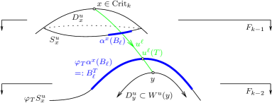
Figure 12: Isolated flow lines $u^{\ell}$ and embedded balls $\alpha^{x}(B_{\ell})$

The task at hand is to express the action of the triple boundary operator on a generator

$$\Theta_{k}\langle x\rangle:=\bar{\vartheta}^{x}_{*}(\sigma_{\langle x\rangle}a_{k})=[D^{u}_{\langle x\rangle}]\in{\rm H}_{k}(F_{k},F_{k-1})={\rm C}_{k}{\mathcal{F}}$$

of ${\rm C}_{k}{\mathcal{F}}$ in terms of generators $[D^{u}_{y}]\in{\rm C}_{k-1}{\mathcal{F}}$ where the $D^{u}_{y}\subset W^{u}(y)$ are appropriately oriented disks – one for each flow trajectory connecting $x$ to some $y\in{\rm Crit}^{a}_{k-1}$. Recall that $\alpha^{x}=\vartheta^{x}|:\SS^{k-1}\to S^{u}_{x}$ is a diffeomorphism. Abbreviate

$$\bar{\alpha}^{x}:=i^{x}\circ\alpha^{x}:\SS^{k-1}\to S^{u}_{x}\hookrightarrow F_{k-1}$$

and

$$\beta^{x}:=\varphi_{T}\circ\alpha^{x},\qquad\bar{\beta}^{x}:=\iota\circ\beta^{x}:\SS^{k-1}\to\varphi_{T}S^{u}_{x}\hookrightarrow F_{k-1},$$ (58)

where $T\geq 1$ will be defined in (62) below. Use the definition (14) of $\Theta_{k}$, the identity (13) for ${\partial}_{k}^{trip}$, and commutativity of the huge diagram above to obtain the following identities

$$\begin{split}\left({\partial}_{k}^{trip}\Theta_{k}\right)\langle x\rangle&=\left(j_{*}{\partial}i_{*}^{x}\vartheta^{x}_{*}\right)(\sigma_{\langle x\rangle}a_{k})\\ &=\sigma_{\langle x\rangle}\left(j_{*}\bar{\alpha}^{x}_{*}\right)(b_{k-1})\\ &=\sigma_{\langle x\rangle}\left(j_{*}\bar{\beta}^{x}_{*}\right)(b_{k-1})\\ &=\sigma_{\langle x\rangle}\left(\bar{\beta}^{x}_{*}J_{*}\right)(b_{k-1})\\ &=\sum_{y\in{\rm Crit}^{a}_{k-1}}\sum_{u\in m_{xy}}\underbrace{\left(i_{*}^{y}\vartheta^{y}_{*}\right)\left(\sigma_{u_{*}\langle x\rangle}a_{k-1}\right)}_{\Theta_{k-1}(u_{*}\langle x\rangle)}\end{split}$$ (59)

among which only the final one remains to be proved. To start with observe that by the Morse-Smale condition together with index difference one the pre-image

$$\{\xi_{1},\dots,\xi_{N}\}:=(\alpha^{x})^{-1}\left(\bigcup_{y\in{\rm Crit}_{k-1}^{a}}W^{s}(y)\right)\cong\bigcup_{y\in{\rm Crit}_{k-1}^{a}}m_{xy}$$

is a finite subset of $\SS^{k-1}$ which parametrizes the set of (unparametrized) heat flow lines running from $x$ to some critical point of Morse index $k-1$; cf. (9) and [28, Prop. 1]. We denote by $u^{\ell}$ the (unique) heat flow trajectory which passes at time $s=0$ through the point $\alpha^{x}(\xi_{\ell})\in W^{u}(x)\cap W^{s}(y)$ where $y=y(\ell):=u^{\ell}(\infty)$ is the corresponding critical point of Morse index $k-1$; see Figure 12. Pick a time $s_{\ell}>0$ such that the point $u^{\ell}(s_{\ell})=\varphi_{s_{\ell}}\alpha^{x}(\xi_{\ell})$ already lies in the ball $B_{y}^{\rho/2}$ about $y$ where the radius $\rho>0$ only depends on the action value $a$; see Lemma 3.1 (Morse-Smale on neighborhoods).

By asymptotic forward existence [27, Thm. 9.14] and strictly decreasing Morse index along connecting orbits due to the Morse-Smale condition, Lemma 3.1, all elements of the punctured sphere $\SS^{k-1}\setminus\{\xi_{1},\dots,\xi_{N}\}$ are mapped under $\alpha^{x}$ to points of $W^{u}(x)$ which asymptotically converge in forward time to some critical point $z$ below level $a$ and of Morse index strictly smaller than $k-1$. But such critical points are contained in $F_{k-2}$; see Definition 1.4. Fix $N$ pairwise disjoint closed balls $\iota^{\ell}:B_{\ell}\hookrightarrow\SS^{k-1}$ centered in $\xi_{\ell}\in\SS^{k-1}$ and sufficiently small such that

$$\varphi_{s_{\ell}}\alpha^{x}(B_{\ell})\subset B^{\rho}_{y(\ell)}\qquad,\ell=1,\dots,N=\sum_{y\in{\rm Crit}^{a}_{k-1}}\mathopen{|}m_{xy}\mathclose{|}.$$ (60)

The canonical orientation of $\SS^{k-1}$ induces a canonical orientation of $B_{\ell}$. Throughout we denote by $B_{\ell}$ the ball equipped with its canonical orientation.

Associated to the closed subset $\overline{F_{k-2}}\subset\Lambda^{a}M$, see (54), there is the continuous entrance time function ${\mathcal{T}}_{\overline{F_{k-2}}}:\Lambda^{a}M\to[0,\infty]$. The function

$$\begin{split}f:\SS^{*}=\SS^{k-1}\setminus\cup_{\ell}\,{\rm int\,}B_{\ell}&\to[0,\infty),\\ \xi&\mapsto{\mathcal{T}}_{\overline{F_{k-2}}}\left(\alpha^{x}(\xi)\right)\end{split}$$ (61)

is continuous and also pointwise finite. Hence by compactness of its domain, that is the punched sphere $\SS^{*}$, the function $f$ admits a maximum. (Note that $F_{k-2}=F_{-1}=\emptyset$ in the case $k=1$.) Consider the instants of time

$$T:=\max\left\{T_{k},s_{x},1+\max f\right\},\qquad s_{x}:=\max\{s_{1},\dots,s_{N}\},$$ (62)

which come with the following consequences. Firstly, by (57) there is the crucial inclusion $\varphi_{T}S^{u}_{x}\subset N_{k-1}\cup F_{k-2}$. This inclusion, together with (43), (44), (60), and the facts that $N_{k-1}=\cup_{z}N_{z}$ and $N_{z}\subset B_{z}^{\rho}$, implies that

$$u^{\ell}(T)\in N_{y(\ell)},\qquad B^{T}_{\ell}:=\varphi_{T}\alpha^{x}(B_{\ell})\subset N_{y(\ell)}\cup F_{k-2}.$$ (63)

Secondly, the image $\varphi_{T}(S^{u}_{x})$ of the map $\bar{\beta}^{x}$ largely lies downtown in $F_{k-2}$ except for (small neighborhoods of) the points $u^{\ell}(T)$ each of which gets stuck at a critical point $y=y(\ell):=u^{\ell}(+\infty)\in{\rm Crit}^{a}_{k-1}$; see Figure 12. Via the isotopy $\{\varphi_{\lambda T}\circ\bar{\alpha}^{x}\}_{\lambda\in[0,1]}$ the map $\bar{\alpha}^{x}$ is homotopic to $\bar{\beta}^{x}$ in $F_{k-1}$. Thus $[S^{u}_{x}]=\bar{\alpha}^{x}_{*}([\SS^{k-1}])=\bar{\beta}^{x}_{*}([\SS^{k-1}])=[\varphi_{T}S^{u}_{x}]$ as elements of ${\rm H}_{k-1}(F_{k-1})$ by the homotopy axiom of singular homology. Most importantly, the map $\bar{\beta}^{x}$ is well defined as a map between the pairs of spaces indicated in the following diagram.

Fix for every $\ell$ an orientation preserving diffeomorphism $\theta^{\ell}:{\mathbb{D}}^{k-1}_{\langle\mathrm{can}\rangle}\to B_{\ell}$ and consider the commutative diagram of maps of pairs

$$\begin{gathered}\lx@xy@svg{\hbox{\raise 0.0pt\hbox{\kern 26.24446pt\hbox{\ignorespaces\ignorespaces\ignorespaces\hbox{\vtop{\kern 0.0pt\offinterlineskip\halign{\entry@#!@&&\entry@@#!@\cr&&\\&&\crcr}}}\ignorespaces{\hbox{\kern-26.24446pt\raise 0.0pt\hbox{\hbox{\kern 0.0pt\raise 0.0pt\hbox{\hbox{\kern 3.0pt\raise 0.0pt\hbox{$\textstyle{({\mathbb{D}}^{k-1},\SS^{k-2})\ignorespaces\ignorespaces\ignorespaces\ignorespaces}$}}}}}}}\ignorespaces\ignorespaces\ignorespaces\ignorespaces{}{\hbox{\lx@xy@droprule}}\ignorespaces\ignorespaces\ignorespaces{\hbox{\kern-10.95277pt\raise-20.63887pt\hbox{{}\hbox{\kern 0.0pt\raise 0.0pt\hbox{\hbox{\kern 3.0pt\hbox{\hbox{\kern 0.0pt\raise-3.125pt\hbox{$\scriptstyle{\theta^{\ell}}$}}}\kern 3.0pt}}}}}}\ignorespaces{\hbox{\kern 0.0pt\raise-30.77774pt\hbox{\hbox{\kern 0.0pt\raise 0.0pt\hbox{\lx@xy@tip{1}\lx@xy@tip{-1}}}}}}{\hbox{\lx@xy@droprule}}{\hbox{\lx@xy@droprule}}{\hbox{\kern 87.02815pt\raise 0.0pt\hbox{\hbox{\kern 0.0pt\raise 0.0pt\hbox{\hbox{\kern 3.0pt\raise 0.0pt\hbox{$\textstyle{\SS^{k-1}\ignorespaces\ignorespaces\ignorespaces\ignorespaces\ignorespaces\ignorespaces\ignorespaces\ignorespaces}$}}}}}}}\ignorespaces\ignorespaces\ignorespaces\ignorespaces{}{\hbox{\lx@xy@droprule}}\ignorespaces\ignorespaces\ignorespaces{\hbox{\kern 88.90804pt\raise-20.63887pt\hbox{{}\hbox{\kern 0.0pt\raise 0.0pt\hbox{\hbox{\kern 3.0pt\hbox{\hbox{\kern 0.0pt\raise-2.39166pt\hbox{$\scriptstyle{J}$}}}\kern 3.0pt}}}}}}\ignorespaces{\hbox{\kern 99.46289pt\raise-29.49998pt\hbox{\hbox{\kern 0.0pt\raise 0.0pt\hbox{\lx@xy@tip{1}\lx@xy@tip{-1}}}}}}{\hbox{\lx@xy@droprule}}{\hbox{\lx@xy@droprule}}\ignorespaces\ignorespaces\ignorespaces\ignorespaces{}{\hbox{\lx@xy@droprule}}\ignorespaces\ignorespaces\ignorespaces{\hbox{\kern 131.38882pt\raise 6.95277pt\hbox{{}\hbox{\kern 0.0pt\raise 0.0pt\hbox{\hbox{\kern 3.0pt\hbox{\hbox{\kern 0.0pt\raise-2.5861pt\hbox{$\scriptstyle{\bar{\beta}^{x}=\iota\varphi_{T}\alpha^{x}}$}}}\kern 3.0pt}}}}}}\ignorespaces{\hbox{\kern 187.97021pt\raise 0.0pt\hbox{\hbox{\kern 0.0pt\raise 0.0pt\hbox{\lx@xy@tip{1}\lx@xy@tip{-1}}}}}}{\hbox{\lx@xy@droprule}}{\hbox{\lx@xy@droprule}}{\hbox{\kern 187.97021pt\raise 0.0pt\hbox{\hbox{\kern 0.0pt\raise 0.0pt\hbox{\hbox{\kern 3.0pt\raise 0.0pt\hbox{$\textstyle{F_{k-1}\ignorespaces\ignorespaces\ignorespaces\ignorespaces}$}}}}}}}\ignorespaces\ignorespaces\ignorespaces\ignorespaces{}{\hbox{\lx@xy@droprule}}\ignorespaces\ignorespaces\ignorespaces{\hbox{\kern 198.75911pt\raise-20.63887pt\hbox{{}\hbox{\kern 0.0pt\raise 0.0pt\hbox{\hbox{\kern 3.0pt\hbox{\hbox{\kern 0.0pt\raise-1.62779pt\hbox{$\scriptstyle{j}$}}}\kern 3.0pt}}}}}}\ignorespaces{\hbox{\kern 198.75911pt\raise-30.77774pt\hbox{\hbox{\kern 0.0pt\raise 0.0pt\hbox{\lx@xy@tip{1}\lx@xy@tip{-1}}}}}}{\hbox{\lx@xy@droprule}}{\hbox{\lx@xy@droprule}}{\hbox{\kern-21.35246pt\raise-41.27774pt\hbox{\hbox{\kern 0.0pt\raise 0.0pt\hbox{\hbox{\kern 3.0pt\raise 0.0pt\hbox{$\textstyle{\left(B_{\ell},{\partial}B_{\ell}\right)\ignorespaces\ignorespaces\ignorespaces\ignorespaces}$}}}}}}}\ignorespaces\ignorespaces\ignorespaces\ignorespaces{}{\hbox{\lx@xy@droprule}}\ignorespaces\ignorespaces\ignorespaces{\hbox{\kern 34.15932pt\raise-36.07635pt\hbox{{}\hbox{\kern 0.0pt\raise 0.0pt\hbox{\hbox{\kern 3.0pt\hbox{\hbox{\kern 0.0pt\raise-2.20139pt\hbox{$\scriptstyle{\iota^{\ell}\qquad\quad}$}}}\kern 3.0pt}}}}}}\ignorespaces{\hbox{\kern 50.24446pt\raise-41.27774pt\hbox{\hbox{\kern 0.0pt\raise 0.0pt\hbox{\lx@xy@tip{1}\lx@xy@tip{-1}}}}}}{\hbox{\lx@xy@droprule}}{\hbox{\lx@xy@droprule}}{\hbox{\kern 50.24446pt\raise-41.27774pt\hbox{\hbox{\kern 0.0pt\raise 0.0pt\hbox{\hbox{\kern 3.0pt\raise 0.0pt\hbox{$\textstyle{\left(\SS^{k-1},\SS^{k-1}\setminus\cup_{\ell}\,{\rm int\,}B_{\ell}\right)\ignorespaces\ignorespaces\ignorespaces\ignorespaces}$}}}}}}}\ignorespaces\ignorespaces\ignorespaces\ignorespaces{}{\hbox{\lx@xy@droprule}}\ignorespaces\ignorespaces\ignorespaces{\hbox{\kern 138.96793pt\raise-35.0083pt\hbox{{}\hbox{\kern 0.0pt\raise 0.0pt\hbox{\hbox{\kern 3.0pt\hbox{\hbox{\kern 0.0pt\raise-3.26944pt\hbox{$\scriptstyle{\quad\bar{\beta}^{x}}$}}}\kern 3.0pt}}}}}}\ignorespaces{\hbox{\kern 172.68132pt\raise-41.27774pt\hbox{\hbox{\kern 0.0pt\raise 0.0pt\hbox{\lx@xy@tip{1}\lx@xy@tip{-1}}}}}}{\hbox{\lx@xy@droprule}}{\hbox{\lx@xy@droprule}}{\hbox{\kern 172.68132pt\raise-41.27774pt\hbox{\hbox{\kern 0.0pt\raise 0.0pt\hbox{\hbox{\kern 3.0pt\raise 0.0pt\hbox{$\textstyle{(F_{k-1},F_{k-2}).}$}}}}}}}\ignorespaces}}}}\ignorespaces\end{gathered} \textstyle{({\mathbb{D}}^{k-1},\SS^{k-2})\ignorespaces\ignorespaces\ignorespaces\ignorespaces} \scriptstyle{\theta^{\ell}} \textstyle{\SS^{k-1}\ignorespaces\ignorespaces\ignorespaces\ignorespaces\ignorespaces\ignorespaces\ignorespaces\ignorespaces} \scriptstyle{J} \scriptstyle{\bar{\beta}^{x}=\iota\varphi_{T}\alpha^{x}} \textstyle{F_{k-1}\ignorespaces\ignorespaces\ignorespaces\ignorespaces} \scriptstyle{j} \textstyle{\left(B_{\ell},{\partial}B_{\ell}\right)\ignorespaces\ignorespaces\ignorespaces\ignorespaces} \scriptstyle{\iota^{\ell}\qquad\quad} \textstyle{\left(\SS^{k-1},\SS^{k-1}\setminus\cup_{\ell}\,{\rm int\,}B_{\ell}\right)\ignorespaces\ignorespaces\ignorespaces\ignorespaces} \scriptstyle{\quad\bar{\beta}^{x}} \textstyle{(F_{k-1},F_{k-2}).} \textstyle{({\mathbb{D}}^{k-1},\SS^{k-2})\ignorespaces\ignorespaces\ignorespaces\ignorespaces} \scriptstyle{\theta^{\ell}} \textstyle{\SS^{k-1}\ignorespaces\ignorespaces\ignorespaces\ignorespaces\ignorespaces\ignorespaces\ignorespaces\ignorespaces} \scriptstyle{J} \scriptstyle{\bar{\beta}^{x}=\iota\varphi_{T}\alpha^{x}} \textstyle{F_{k-1}\ignorespaces\ignorespaces\ignorespaces\ignorespaces} \scriptstyle{j} \textstyle{\left(B_{\ell},{\partial}B_{\ell}\right)\ignorespaces\ignorespaces\ignorespaces\ignorespaces} \scriptstyle{\iota^{\ell}\qquad\quad} \textstyle{\left(\SS^{k-1},\SS^{k-1}\setminus\cup_{\ell}\,{\rm int\,}B_{\ell}\right)\ignorespaces\ignorespaces\ignorespaces\ignorespaces} \scriptstyle{\quad\bar{\beta}^{x}} \textstyle{(F_{k-1},F_{k-2}).}$$ (64)

Here $J$ and $j$ denote inclusions of pairs $X=(X,\emptyset)\mapsto(X,A)$. The identity

$$J_{*}(b_{k-1})=\sum_{\ell=1}^{N}\bar{\theta}^{\ell}_{*}(a_{k-1}),\qquad\bar{\theta}^{\ell}:=\iota^{\ell}\theta^{\ell},$$ (65)

provided by [1, Exc. 2.12] proves the first of the two identities

$$\begin{split}\sigma_{\langle x\rangle}\cdot\bigl{(}\bar{\beta}^{x}_{*}J_{*}\bigr{)}(b_{k-1})&=\sigma_{\langle x\rangle}\cdot\sum_{\ell=1}^{N}\left(\bar{\beta}^{x}\bar{\theta}^{\ell}\right)_{*}(a_{k-1})\\ &=\sum_{\ell=1}^{N}\sigma_{u^{\ell}_{*}\langle x\rangle}\cdot\bar{\vartheta}^{y}_{*}(a_{k-1}).\end{split}$$ (66)

To conclude the proof of (66), thus of (59), hence of Theorem 1.5, it remains to prove that the maps

$$\sigma_{\langle x\rangle}\cdot(\bar{\beta}^{x}\bar{\theta}^{\ell})_{*}\;\text{and}\;\sigma_{u^{\ell}_{*}\langle x\rangle}\cdot\bar{\vartheta}^{y}_{*}:{\rm H}_{k-1}({\mathbb{D}}^{k-1},\SS^{k-2})\to{\rm H}_{k-1}(F_{k-1},F_{k-2})$$ (67)

coincide on the positive generator $a_{k-1}$. By definition (40) of the orientation reversing diffeomorphism $\mu={\rm diag}(-1,1,\dots,1)\in{\mathcal{L}}({\mathbb{R}}^{k-1})$ and $\kappa_{\langle x\rangle}\in\{0,1\}$ this holds true if the by $\mu$ pre-composed maps of pairs (illustrated by Figure 13)

$$\bar{\beta}^{x}\bar{\theta}^{\ell}\mu^{\kappa_{\langle x\rangle}}\;\;\text{and}\;\;\bar{\vartheta}^{y}\mu^{\kappa_{\ell}}\;:\;({\mathbb{D}}^{k-1},\SS^{k-2})\to(F_{k-1},F_{k-2}),\qquad\kappa_{\ell}:=\kappa_{u^{\ell}_{*}\langle x\rangle},$$

are isotopic, thus homotopic among orientation preserving maps. The proof takes two steps. First we isotop (a relevant part of) the map $\bar{\beta}^{x}\bar{\theta}^{\ell}$ to $\bar{\vartheta}^{y}$, then in step two we verify that all chosen orientations are preserved.

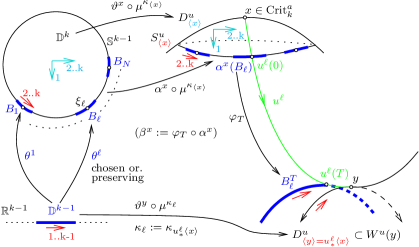
Figure 13: All maps are orientation preserving by choice of the exponents $\kappa$

Step 1 (Isotopy). We construct an isotopy of maps of pairs

$$({\mathbb{D}}^{k-1},\SS^{k-2})\to(N_{y}\cup F_{k-2},F_{k-2})\subset(F_{k-1},F_{k-2})$$

between (relevant parts of) the embedded disks

$$\bar{\beta}^{x}\bar{\theta}^{\ell}({\mathbb{D}}^{k-1})=\varphi_{T}\alpha^{x}(B_{\ell})=:B^{T}_{\ell}\quad\text{and}\quad\bar{\vartheta}^{y}({\mathbb{D}}^{k-1})=D^{u}_{y}\quad\text{where $y=u^{\ell}(\infty)$.}$$

Remarkably at this very late stage of the whole project eventually the forward analogue of the Backward $\lambda$-Lemma [31, Thm. 1] enters as a crucial tool. This is a local result valid in a neighborhood of a hyperbolic fixed point. We assume without loss of generality that the forward $\lambda$-Lemma applies on the whole domain of our usual local coordinates $\Phi^{-1}$ near any of the finitely many critical points on $\Lambda^{a}M$. From now on we fix a local parametrization $\Phi:T_{y}\Lambda M=X=X^{-}\oplus X^{+}\supset B^{u}\times B^{+}\to\Lambda M$ near $y=y(\ell)$ and use our usual conventions concerning local notations; see Hypothesis 2.2 and Figure 14. In particular, the local flow is denoted by $\phi$ and $S^{u}_{\varepsilon}$ abbreviates the descending sphere $S^{u}_{\varepsilon}(y)$. However, we will not change notations such as $N_{y}$, $L_{k-1}$, $F_{k-2}$ etc.

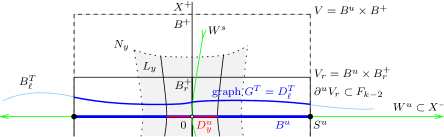
Figure 14: Isotopy $\{{\rm graph}\>\lambda G^{T}\}_{\lambda\in[0,1]}$ between $D^{T}_{\ell}$ and $B^{u}\supset D^{u}_{y}$

Observe that $\phi_{-2\tau}S^{u}_{\varepsilon}\subset L_{y}\subset L_{k-1}\subset F_{k-2}$ where the three inclusions hold by Proposition 2.13, (45), and (47), respectively. Thus

$$W^{u}\setminus D^{u}_{y}=\phi_{(-2\tau,\infty)}S^{u}_{\varepsilon}=\phi_{(0,\infty)}(\phi_{-2\tau}S^{u}_{\varepsilon})\subset F_{k-2}$$ (68)

by semi-flow invariance of $F_{k-2}$. Because $N_{y}\subset B^{\rho}_{y}\subset B^{2\rho}_{y}\subset B^{u}\times B^{+}$ by Hypothesis 3.2, the $(k-1)$-sphere $S^{u}:={\partial}B^{u}\subset W^{u}$ is disjoint to $N_{y}$, thus to $D^{u}_{y}$. In fact, the distance between $S^{u}$ and $N_{y}$ is at least $\rho$. Consequently $S^{u}\subset W^{u}\setminus D^{u}_{u}\subset F_{k-2}$ by (68). Therefore by openness of $F_{k-2}$ and compactness of its subset $S^{u}$ there is a radius $r\in(0,1)$ such that the family $S^{u}\times B^{+}_{r}$ of radius $r$ balls $B^{+}_{r}$ about $0\in X^{+}$ is contained in $F_{k-2}$. To summarize

$${\partial}^{u}V_{r}:=S^{u}\times B^{+}_{r}\subset F_{k-2},\qquad{\partial}^{u}V_{r}\cap N_{y}=\emptyset.$$ (69)

The forward $\lambda$-Lemma asserts that for every sufficiently large time $T$ the part

$$D^{T}_{\ell}:=B^{T}_{\ell}\cap\left(B^{u}\times B^{+}\right)={\rm graph}\;G^{T},\qquad G^{T}\in C^{1}(B^{u},B^{+}),$$

of the disk $B^{T}_{\ell}=\varphi_{T}\alpha^{x}(B_{\ell})=\beta^{x}\theta^{\ell}({\mathbb{D}}^{k-1})$ inside $B^{u}\times B^{+}$ is the graph of a $C^{1}$ map $G^{T}:B^{u}\to B^{+}$ whose $C^{1}$ norm converges to zero, as $T\to\infty$. Thus choose $T$ in (62) larger, if necessary, to obtain that $\mathopen{\|}G^{T}\mathclose{\|}_{C^{1}}<r$. Then, as elements of ${\rm H}_{k-1}(F_{k-1},F_{k-2})$, the following classes are equal

$$\begin{split}\left(\bar{\beta}^{x}\bar{\theta}^{\ell}\right)_{*}[{\mathbb{D}}^{k-1}]=[B^{T}_{\ell}]=[D^{T}_{\ell}]=[B^{u}]=[D^{u}_{y}]=\left(\bar{\vartheta}^{y}\right)_{*}[{\mathbb{D}}^{k-1}].\end{split}$$

Here the first identity is just by definition of the maps. The class of $B^{T}_{\ell}$ is well defined in relative homology by (64) building on definition (62) of $T$. The part of the disk $B^{T}_{\ell}$ in $V$ is $D^{T}_{\ell}=G^{T}(B^{u})$ whose boundary lies in ${\partial}^{u}V_{r}$, hence in $F_{k-2}$ by (69). So $D^{T}_{\ell}$ is a cycle relative $F_{k-2}$. On the other hand, its complement $B^{T}_{\ell}\setminus D^{T}_{\ell}$ lies outside $V$, hence outside $N_{y}$, and therefore in $F_{k-2}$ by (63). Consequently the classes of $B^{T}_{\ell}$ and $D^{T}_{\ell}$ coincide relative $F_{k-2}$. Concerning identity three observe that $D^{T}_{\ell}$ and $B^{u}$ are isotopic through the embedded disks ${\rm graph}\>\lambda G^{T}$, for $\lambda\in[0,1]$, whose boundaries lie in ${\partial}^{u}V_{r}\subset F_{k-2}$. Identity four uses that $B^{u}\setminus D^{u}_{y}\subset W^{u}\setminus D^{u}_{y}\subset F_{k-2}$ by (68). The final identity five holds by choice of the diffeomorphism $\vartheta^{x}$ in (36).
This proves (67) modulo signs. So it only remains to study orientations.

Step 2 (Orientations). To prove (67) recall the definition of the transport $u^{\ell}_{*}\langle x\rangle$ of the orientation $\langle x\rangle$ of $W^{u}(x)$ along the heat flow trajectory $u^{\ell}$ between the critical points $x$ and $y:=u^{\ell}(+\infty)$ towards an orientation of $W^{u}(y)$. By Lemma 2.9 for small ${\varepsilon}>0$ the ascending disk $W^{s}_{\varepsilon}(y)$ is a codimension $(k-1)$ submanifold of $\Lambda^{a}M$. Choosing $T$ larger, if necessary, the point $p_{\ell}:=u^{\ell}(T)$ which anyway lies on the trajectory $u^{\ell}$ from $x$ to $y$ moves closer to $y$ and eventually lies in $W^{s}_{\varepsilon}(y)$. By the Morse-Smale condition the orthogonal complement $T_{p_{\ell}}W^{s}_{\varepsilon}(y)^{\perp}$ is a subspace of $T_{p_{\ell}}W^{u}(x)$. The latter splits as a direct sum of subspaces

$$T_{p_{\ell}}W^{u}(x)={\mathbb{R}}\left(\tfrac{d}{ds}\varphi_{s}p_{\ell}\right)\oplus T_{p_{\ell}}W^{s}_{\varepsilon}(y)^{\perp},\qquad p_{\ell}:=u^{\ell}(T).$$ (70)

Since two of the three vector spaces are oriented, namely by $\langle x\rangle$ and by the downward flow, the third space inherits an orientation as well. Thereby providing a co-orientation along all of the (contractible) ascending disk $W^{s}_{\varepsilon}(y)$, in particular, at the point $y$ itself. But $T_{y}W^{s}_{\varepsilon}(y)^{\perp}=T_{y}W^{u}(y)$, so the co-orientation determines an orientation of the unstable manifold $W^{u}(y)$ called the push-forward orientation of $\langle x\rangle$ along the flow line $u^{\ell}$ and denoted by $u^{\ell}_{*}\langle x\rangle$.

On the other hand, the boundary orientation of $\SS^{k-1}$ is determined by an outward pointing vector field and the canonical orientation of ${\mathbb{D}}^{k}$. Given the orientation $\langle x\rangle$ of $W^{u}(x)$, the boundary orientation of the $(k-1)$-sphere $S^{u}_{x}={\partial}D^{u}_{x}\subset W^{u}(x)$ arises the same way using the (outward pointing) downward gradient vector field. But the sign $\sigma_{\langle x\rangle}$ of the diffeomorphism $\vartheta^{x}$ has been chosen in (39) precisely to make $\vartheta^{x}\circ\mu^{\kappa_{\langle x\rangle}}$ and its restriction to the boundary preserve these orientations. In particular, there is the oriented direct sum

$$\left\langle T_{p_{\ell}}W^{u}(x)\right\rangle_{\langle x\rangle}=\left\langle{\mathbb{R}}\left(\tfrac{d}{ds}\varphi_{s}p_{\ell}\right)\right\rangle_{\text{flow}}\oplus\left\langle T_{p_{\ell}}B_{\ell}^{T}\right\rangle_{\varphi_{T}\alpha^{x}\mu^{\kappa_{\langle x\rangle}}}.$$ (71)

Compare these orientations with the ones in (70), which determine $u^{\ell}_{*}\langle x\rangle$, to obtain that $(\varphi_{T}\bar{\alpha}^{x}\mu^{\kappa_{\langle x\rangle}})_{*}({\mathbb{D}}^{k}_{\langle\mathrm{can}\rangle})=u^{\ell}_{*}\langle x\rangle=(\bar{\vartheta}^{y}\mu^{\kappa_{\ell}})_{*}({\mathbb{D}}^{k}_{\langle\mathrm{can}\rangle})$ where $\kappa_{\ell}=\kappa_{u^{\ell}_{*}\langle x\rangle}$ and where the second identity holds by the very definition of the sign $\sigma_{u^{\ell}_{*}\langle x\rangle}$. ∎

3.4 The natural isomorphism on homology

Theorem 3.7.

Suppose $M$ is simply connected. Assume ${\mathcal{V}}:{\mathcal{L}}M\to{\mathbb{R}}$ is a perturbation that satisfies (V0)–(V3) in [28] and ${\mathcal{S}}_{\mathcal{V}}$ is Morse-Smale below a regular value $a\in{\mathbb{R}}$. Then there is a natural isomorphism

$$\Psi^{a}_{*}:{\rm HM}^{a}_{*}(\Lambda M,{\mathcal{S}}_{\mathcal{V}})\to\mathrm{H}_{*}(\Lambda^{a}M)$$

which commutes with the homomorphisms ${\rm HM}^{b}_{*}(\Lambda M,{\mathcal{S}}_{\mathcal{V}})\to{\rm HM}^{a}_{*}(\Lambda M,{\mathcal{S}}_{\mathcal{V}})$ and $\mathrm{H}_{*}(\Lambda^{b}M)\to\mathrm{H}_{*}(\Lambda^{a}M)$ for $b<a$.

Proof of Theorem 3.7.

Suppose ${\mathcal{S}}_{\mathcal{V}}$ is Morse-Smale below level $a$ and $b\leq a$ are regular values. Consider the Morse filtrations ${\mathcal{F}}(\Lambda^{b}M)\hookrightarrow{\mathcal{F}}(\Lambda^{a}M)$ provided by (47) and (51). Then the desired natural isomorphism is the composition of the two horizontal natural isomorphisms in the following diagram.

$$\begin{split}\lx@xy@svg{\hbox{\raise 0.0pt\hbox{\kern 42.68138pt\hbox{\ignorespaces\ignorespaces\ignorespaces\hbox{\vtop{\kern 0.0pt\offinterlineskip\halign{\entry@#!@&&\entry@@#!@\cr&&\\&&\crcr}}}\ignorespaces{\hbox{\kern-42.68138pt\raise 0.0pt\hbox{\hbox{\kern 0.0pt\raise 0.0pt\hbox{\hbox{\kern 3.0pt\raise 0.0pt\hbox{$\textstyle{\Psi^{a}_{*}\,:\,{\rm HM}_{*}^{a}(\Lambda M,{\mathcal{S}}_{\mathcal{V}})\ignorespaces\ignorespaces\ignorespaces\ignorespaces}$}}}}}}}\ignorespaces\ignorespaces\ignorespaces\ignorespaces{}{\hbox{\lx@xy@droprule}}\ignorespaces\ignorespaces\ignorespaces{\hbox{\kern 34.85068pt\raise-6.15pt\hbox{{}\hbox{\kern 0.0pt\raise 0.0pt\hbox{\hbox{\kern 3.0pt\hbox{\hbox{\kern 0.0pt\raise-1.75pt\hbox{$\scriptstyle{\hskip 11.38092pt\cong}$}}}\kern 3.0pt}}}}}}\ignorespaces\ignorespaces\ignorespaces{\hbox{\kern 32.52016pt\raise 6.69722pt\hbox{{}\hbox{\kern 0.0pt\raise 0.0pt\hbox{\hbox{\kern 3.0pt\hbox{\hbox{\kern 0.0pt\raise-1.94722pt\hbox{$\scriptstyle{\hskip 9.95863pt[\Theta_{*}^{a}]}$}}}\kern 3.0pt}}}}}}\ignorespaces{\hbox{\kern 66.68138pt\raise 0.0pt\hbox{\hbox{\kern 0.0pt\raise 0.0pt\hbox{\lx@xy@tip{1}\lx@xy@tip{-1}}}}}}{\hbox{\lx@xy@droprule}}{\hbox{\lx@xy@droprule}}{\hbox{\kern 66.68138pt\raise 0.0pt\hbox{\hbox{\kern 0.0pt\raise 0.0pt\hbox{\hbox{\kern 3.0pt\raise 0.0pt\hbox{$\textstyle{{\rm H}_{*}{\mathcal{F}}\left(\Lambda^{a}M\right)\ignorespaces\ignorespaces\ignorespaces\ignorespaces}$}}}}}}}\ignorespaces\ignorespaces\ignorespaces\ignorespaces{}{\hbox{\lx@xy@droprule}}\ignorespaces\ignorespaces\ignorespaces{\hbox{\kern 122.1835pt\raise-6.15pt\hbox{{}\hbox{\kern 0.0pt\raise 0.0pt\hbox{\hbox{\kern 3.0pt\hbox{\hbox{\kern 0.0pt\raise-1.75pt\hbox{$\scriptstyle{\cong\hskip 8.5359pt}$}}}\kern 3.0pt}}}}}}\ignorespaces\ignorespaces\ignorespaces{\hbox{\kern 117.45541pt\raise 9.68504pt\hbox{{}\hbox{\kern 0.0pt\raise 0.0pt\hbox{\hbox{\kern 3.0pt\hbox{\hbox{\kern 0.0pt\raise 1.43504pt\hbox{$\scriptstyle{(\ref{eq:isomorphism-cellular-singular})\hskip 11.38092pt}$}}}\kern 3.0pt}}}}}}\ignorespaces{\hbox{\kern 141.9832pt\raise 0.0pt\hbox{\hbox{\kern 0.0pt\raise 0.0pt\hbox{\lx@xy@tip{1}\lx@xy@tip{-1}}}}}}{\hbox{\lx@xy@droprule}}{\hbox{\lx@xy@droprule}}{\hbox{\kern 141.9832pt\raise 0.0pt\hbox{\hbox{\kern 0.0pt\raise 0.0pt\hbox{\hbox{\kern 3.0pt\raise 0.0pt\hbox{$\textstyle{\mathrm{H}_{*}(\{{\mathcal{S}}_{\mathcal{V}}\leq a\})}$}}}}}}}{\hbox{\kern-42.403pt\raise-40.9083pt\hbox{\hbox{\kern 0.0pt\raise 0.0pt\hbox{\hbox{\kern 3.0pt\raise 0.0pt\hbox{$\textstyle{\Psi^{b}_{*}\,:\,{\rm HM}_{*}^{b}(\Lambda M,{\mathcal{S}}_{\mathcal{V}})\ignorespaces\ignorespaces\ignorespaces\ignorespaces\ignorespaces\ignorespaces\ignorespaces\ignorespaces}$}}}}}}}\ignorespaces\ignorespaces\ignorespaces\ignorespaces{}{\hbox{\lx@xy@droprule}}\ignorespaces\ignorespaces\ignorespaces{\hbox{\kern-10.47755pt\raise-20.45415pt\hbox{{}\hbox{\kern 0.0pt\raise 0.0pt\hbox{\hbox{\kern 3.0pt\hbox{\hbox{\kern 0.0pt\raise-1.04167pt\hbox{$\scriptstyle{\iota_{*}}$}}}\kern 3.0pt}}}}}}\ignorespaces{\hbox{\kern 0.0pt\raise-5.5pt\hbox{\hbox{\kern 0.0pt\raise 0.0pt\hbox{\lx@xy@tip{1}\lx@xy@tip{-1}}}}}}{\hbox{\lx@xy@droprule}}{\hbox{\lx@xy@droprule}}\ignorespaces\ignorespaces\ignorespaces\ignorespaces{}{\hbox{\lx@xy@droprule}}\ignorespaces\ignorespaces\ignorespaces{\hbox{\kern 34.85068pt\raise-47.05829pt\hbox{{}\hbox{\kern 0.0pt\raise 0.0pt\hbox{\hbox{\kern 3.0pt\hbox{\hbox{\kern 0.0pt\raise-1.75pt\hbox{$\scriptstyle{\hskip 11.38092pt\cong}$}}}\kern 3.0pt}}}}}}\ignorespaces\ignorespaces\ignorespaces{\hbox{\kern 32.52016pt\raise-33.94719pt\hbox{{}\hbox{\kern 0.0pt\raise 0.0pt\hbox{\hbox{\kern 3.0pt\hbox{\hbox{\kern 0.0pt\raise-2.2111pt\hbox{$\scriptstyle{\hskip 9.95863pt[\Theta_{*}^{b}]}$}}}\kern 3.0pt}}}}}}\ignorespaces{\hbox{\kern 66.95976pt\raise-40.9083pt\hbox{\hbox{\kern 0.0pt\raise 0.0pt\hbox{\lx@xy@tip{1}\lx@xy@tip{-1}}}}}}{\hbox{\lx@xy@droprule}}{\hbox{\lx@xy@droprule}}{\hbox{\kern 66.95976pt\raise-40.9083pt\hbox{\hbox{\kern 0.0pt\raise 0.0pt\hbox{\hbox{\kern 3.0pt\raise 0.0pt\hbox{$\textstyle{{\rm H}_{*}{\mathcal{F}}\left(\Lambda^{b}M\right)\ignorespaces\ignorespaces\ignorespaces\ignorespaces\ignorespaces\ignorespaces\ignorespaces\ignorespaces}$}}}}}}}\ignorespaces\ignorespaces\ignorespaces\ignorespaces{}{\hbox{\lx@xy@droprule}}\ignorespaces\ignorespaces\ignorespaces{\hbox{\kern 122.1835pt\raise-47.05829pt\hbox{{}\hbox{\kern 0.0pt\raise 0.0pt\hbox{\hbox{\kern 3.0pt\hbox{\hbox{\kern 0.0pt\raise-1.75pt\hbox{$\scriptstyle{\cong\hskip 8.5359pt}$}}}\kern 3.0pt}}}}}}\ignorespaces\ignorespaces\ignorespaces{\hbox{\kern 117.45541pt\raise-31.22325pt\hbox{{}\hbox{\kern 0.0pt\raise 0.0pt\hbox{\hbox{\kern 3.0pt\hbox{\hbox{\kern 0.0pt\raise 1.43504pt\hbox{$\scriptstyle{(\ref{eq:isomorphism-cellular-singular})\hskip 11.38092pt}$}}}\kern 3.0pt}}}}}}\ignorespaces{\hbox{\kern 142.48032pt\raise-40.9083pt\hbox{\hbox{\kern 0.0pt\raise 0.0pt\hbox{\lx@xy@tip{1}\lx@xy@tip{-1}}}}}}{\hbox{\lx@xy@droprule}}{\hbox{\lx@xy@droprule}}\ignorespaces\ignorespaces\ignorespaces\ignorespaces{}{\hbox{\lx@xy@droprule}}\ignorespaces\ignorespaces\ignorespaces{\hbox{\kern 81.85474pt\raise-20.45415pt\hbox{{}\hbox{\kern 0.0pt\raise 0.0pt\hbox{\hbox{\kern 3.0pt\hbox{\hbox{\kern 0.0pt\raise-1.04167pt\hbox{$\scriptstyle{\iota_{*}}$}}}\kern 3.0pt}}}}}}\ignorespaces{\hbox{\kern 92.33229pt\raise-5.5pt\hbox{\hbox{\kern 0.0pt\raise 0.0pt\hbox{\lx@xy@tip{1}\lx@xy@tip{-1}}}}}}{\hbox{\lx@xy@droprule}}{\hbox{\lx@xy@droprule}}{\hbox{\kern 142.48032pt\raise-40.9083pt\hbox{\hbox{\kern 0.0pt\raise 0.0pt\hbox{\hbox{\kern 3.0pt\raise 0.0pt\hbox{$\textstyle{\mathrm{H}_{*}(\{{\mathcal{S}}_{\mathcal{V}}\leq b\})\ignorespaces\ignorespaces\ignorespaces\ignorespaces}$}}}}}}}\ignorespaces\ignorespaces\ignorespaces\ignorespaces{}{\hbox{\lx@xy@droprule}}\ignorespaces\ignorespaces\ignorespaces{\hbox{\kern 161.34305pt\raise-20.45415pt\hbox{{}\hbox{\kern 0.0pt\raise 0.0pt\hbox{\hbox{\kern 3.0pt\hbox{\hbox{\kern 0.0pt\raise-1.04167pt\hbox{$\scriptstyle{\iota_{*}}$}}}\kern 3.0pt}}}}}}\ignorespaces{\hbox{\kern 171.8206pt\raise-5.5pt\hbox{\hbox{\kern 0.0pt\raise 0.0pt\hbox{\lx@xy@tip{1}\lx@xy@tip{-1}}}}}}{\hbox{\lx@xy@droprule}}{\hbox{\lx@xy@droprule}}\ignorespaces}}}}\ignorespaces\end{split} \textstyle{\Psi^{a}_{*}\,:\,{\rm HM}_{*}^{a}(\Lambda M,{\mathcal{S}}_{\mathcal{V}})\ignorespaces\ignorespaces\ignorespaces\ignorespaces} \scriptstyle{\hskip 11.38092pt\cong} \scriptstyle{\hskip 9.95863pt[\Theta_{*}^{a}]} \textstyle{{\rm H}_{*}{\mathcal{F}}\left(\Lambda^{a}M\right)\ignorespaces\ignorespaces\ignorespaces\ignorespaces} \scriptstyle{\cong\hskip 8.5359pt} \scriptstyle{(\ref{eq:isomorphism-cellular-singular})\hskip 11.38092pt} \textstyle{\mathrm{H}_{*}(\{{\mathcal{S}}_{\mathcal{V}}\leq a\})} \textstyle{\Psi^{b}_{*}\,:\,{\rm HM}_{*}^{b}(\Lambda M,{\mathcal{S}}_{\mathcal{V}})\ignorespaces\ignorespaces\ignorespaces\ignorespaces\ignorespaces\ignorespaces\ignorespaces\ignorespaces} \scriptstyle{\iota_{*}} \scriptstyle{\hskip 11.38092pt\cong} \scriptstyle{\hskip 9.95863pt[\Theta_{*}^{b}]} \textstyle{{\rm H}_{*}{\mathcal{F}}\left(\Lambda^{b}M\right)\ignorespaces\ignorespaces\ignorespaces\ignorespaces\ignorespaces\ignorespaces\ignorespaces\ignorespaces} \scriptstyle{\cong\hskip 8.5359pt} \scriptstyle{(\ref{eq:isomorphism-cellular-singular})\hskip 11.38092pt} \scriptstyle{\iota_{*}} \textstyle{\mathrm{H}_{*}(\{{\mathcal{S}}_{\mathcal{V}}\leq b\})\ignorespaces\ignorespaces\ignorespaces\ignorespaces} \scriptstyle{\iota_{*}} \textstyle{\Psi^{a}_{*}\,:\,{\rm HM}_{*}^{a}(\Lambda M,{\mathcal{S}}_{\mathcal{V}})\ignorespaces\ignorespaces\ignorespaces\ignorespaces} \scriptstyle{\hskip 11.38092pt\cong} \scriptstyle{\hskip 9.95863pt[\Theta_{*}^{a}]} \textstyle{{\rm H}_{*}{\mathcal{F}}\left(\Lambda^{a}M\right)\ignorespaces\ignorespaces\ignorespaces\ignorespaces} \scriptstyle{\cong\hskip 8.5359pt} \scriptstyle{(\ref{eq:isomorphism-cellular-singular})\hskip 11.38092pt} \textstyle{\mathrm{H}_{*}(\{{\mathcal{S}}_{\mathcal{V}}\leq a\})} \textstyle{\Psi^{b}_{*}\,:\,{\rm HM}_{*}^{b}(\Lambda M,{\mathcal{S}}_{\mathcal{V}})\ignorespaces\ignorespaces\ignorespaces\ignorespaces\ignorespaces\ignorespaces\ignorespaces\ignorespaces} \scriptstyle{\iota_{*}} \scriptstyle{\hskip 11.38092pt\cong} \scriptstyle{\hskip 9.95863pt[\Theta_{*}^{b}]} \textstyle{{\rm H}_{*}{\mathcal{F}}\left(\Lambda^{b}M\right)\ignorespaces\ignorespaces\ignorespaces\ignorespaces\ignorespaces\ignorespaces\ignorespaces\ignorespaces} \scriptstyle{\cong\hskip 8.5359pt} \scriptstyle{(\ref{eq:isomorphism-cellular-singular})\hskip 11.38092pt} \scriptstyle{\iota_{*}} \textstyle{\mathrm{H}_{*}(\{{\mathcal{S}}_{\mathcal{V}}\leq b\})\ignorespaces\ignorespaces\ignorespaces\ignorespaces} \scriptstyle{\iota_{*}}$$

Concerning the left rectangle observe that already both chain complexes, underlying ${\rm HM}_{*}$ and ${\rm H}_{*}{\mathcal{F}}$, are naturally identified for each regular level $b\leq a$ by the chain complex isomorphism $\Theta_{*}^{b}$ – see Theorem B and Theorem 1.5 – which we actually established above for the present class of abstract potentials ${\mathcal{V}}$. Each of the two vertical maps $\iota_{*}$ is induced by the inclusion of the subcomplex associated to $b$. Thus the left rectangle already commutes on the chain level. The right rectangle is due to and commutes by Theorem 3.5. ∎

Proof of Theorem A.

Consider the Morse function ${\mathcal{S}}_{V}$ in Theorem A and pick a regular value $a$. Then the transversality theorem [28, §1.2 Thm. 8] provides, for each regular perturbation $v\in{\mathcal{O}}^{a}_{reg}$, the second of the two natural isomorphisms

$${\rm HM}_{*}^{a}(\Lambda M,{\mathcal{S}}_{V+v})\stackrel{{\scriptstyle\Psi^{a}_{*}}}{{\cong}}\mathrm{H}_{*}(\{{\mathcal{S}}_{V+v}\leq a\})\cong\mathrm{H}_{*}(\{{\mathcal{S}}_{V}\leq a\})$$ (72)

where, of course, the notation ${\mathcal{S}}_{V+v}$ is slightly abusive. The first isomorphism $\Psi^{a}_{*}$ is due to Theorem 3.7 and the second one to [28, §5.2 Prop. 8]. Concerning $\Psi^{a}_{*}$ it is crucial that ${\mathcal{S}}_{V+v}$ is Morse-Smale below level $a$ – which holds by regularity of $v$ – and concerning the second isomorphism that $v$ lies in the radius $r_{a}$ ball ${\mathcal{O}}^{a}$ defined by [28, (62)]. This proves (12), thus the first part of Theorem A.

Now assume that $a<b$ are regular values of ${\mathcal{S}}_{V}$. The set of admissible perturbations ${\mathcal{O}}^{b}$ given by [28, (62)] is a closed ball about zero in a separable Banach space. Pick a regular perturbation $v\in{\mathcal{O}}^{b}_{reg}\subset{\mathcal{O}}^{b}$ whose norm is bounded from above by the constant $\delta^{a}/2$ given by [28, (61)]. In this case $v$ is in the set ${\mathcal{O}}^{a}$ by [28, §5.2 Rmk. 4] and therefore enjoys the properties stated in [28, §5.2 Prop. 8] for both values $a$ and $b$; see also the transversality theorem [28, §1.2 Thm. 8]. Of course, as the perturbed action ${\mathcal{S}}_{V+v}$ is Morse-Smale below level $b$, it is so below level $a$. Hence $v\in{\mathcal{O}}^{a}_{reg}\cap{\mathcal{O}}^{b}_{reg}$ and therefore we obtain, just as above, the horizontal isomorphisms in the diagram

$$\begin{split}\lx@xy@svg{\hbox{\raise 0.0pt\hbox{\kern 35.27022pt\hbox{\ignorespaces\ignorespaces\ignorespaces\hbox{\vtop{\kern 0.0pt\offinterlineskip\halign{\entry@#!@&&\entry@@#!@\cr&&\\&&\crcr}}}\ignorespaces{\hbox{\kern-35.27022pt\raise 0.0pt\hbox{\hbox{\kern 0.0pt\raise 0.0pt\hbox{\hbox{\kern 3.0pt\raise 0.0pt\hbox{$\textstyle{{\rm HM}_{*}^{b}(\Lambda M,{\mathcal{S}}_{V+v})\ignorespaces\ignorespaces\ignorespaces\ignorespaces}$}}}}}}}\ignorespaces\ignorespaces\ignorespaces\ignorespaces{}{\hbox{\lx@xy@droprule}}\ignorespaces\ignorespaces\ignorespaces{\hbox{\kern 39.86877pt\raise 6.55139pt\hbox{{}\hbox{\kern 0.0pt\raise 0.0pt\hbox{\hbox{\kern 3.0pt\hbox{\hbox{\kern 0.0pt\raise-2.62083pt\hbox{$\scriptstyle{\Psi^{b}_{*}}$}}}\kern 3.0pt}}}}}}\ignorespaces{\hbox{\kern 59.76733pt\raise 0.0pt\hbox{\hbox{\kern 0.0pt\raise 0.0pt\hbox{\lx@xy@tip{1}\lx@xy@tip{-1}}}}}}{\hbox{\lx@xy@droprule}}{\hbox{\lx@xy@droprule}}{\hbox{\kern 59.76733pt\raise 0.0pt\hbox{\hbox{\kern 0.0pt\raise 0.0pt\hbox{\hbox{\kern 3.0pt\raise 0.0pt\hbox{$\textstyle{\mathrm{H}_{*}(\{{\mathcal{S}}_{V+v}\leq b\})\ignorespaces\ignorespaces\ignorespaces\ignorespaces}$}}}}}}}\ignorespaces\ignorespaces\ignorespaces\ignorespaces{}{\hbox{\lx@xy@droprule}}\ignorespaces\ignorespaces\ignorespaces{\hbox{\kern 127.53712pt\raise 9.68504pt\hbox{{}\hbox{\kern 0.0pt\raise 0.0pt\hbox{\hbox{\kern 3.0pt\hbox{\hbox{\kern 0.0pt\raise 1.43504pt\hbox{$\scriptstyle{(\ref{eq:comm-tri-h})_{b}}$}}}\kern 3.0pt}}}}}}\ignorespaces{\hbox{\kern 152.4131pt\raise 0.0pt\hbox{\hbox{\kern 0.0pt\raise 0.0pt\hbox{\lx@xy@tip{1}\lx@xy@tip{-1}}}}}}{\hbox{\lx@xy@droprule}}{\hbox{\lx@xy@droprule}}{\hbox{\kern 152.4131pt\raise 0.0pt\hbox{\hbox{\kern 0.0pt\raise 0.0pt\hbox{\hbox{\kern 3.0pt\raise 0.0pt\hbox{$\textstyle{\mathrm{H}_{*}(\{{\mathcal{S}}_{{\mathcal{V}}}\leq b\})}$}}}}}}}{\hbox{\kern-35.27022pt\raise-40.9083pt\hbox{\hbox{\kern 0.0pt\raise 0.0pt\hbox{\hbox{\kern 3.0pt\raise 0.0pt\hbox{$\textstyle{{\rm HM}_{*}^{a}(\Lambda M,{\mathcal{S}}_{V+v})\ignorespaces\ignorespaces\ignorespaces\ignorespaces\ignorespaces\ignorespaces\ignorespaces\ignorespaces}$}}}}}}}\ignorespaces\ignorespaces\ignorespaces\ignorespaces{}{\hbox{\lx@xy@droprule}}\ignorespaces\ignorespaces\ignorespaces{\hbox{\kern 39.66992pt\raise-34.62079pt\hbox{{}\hbox{\kern 0.0pt\raise 0.0pt\hbox{\hbox{\kern 3.0pt\hbox{\hbox{\kern 0.0pt\raise-2.35695pt\hbox{$\scriptstyle{\Psi^{a}_{*}}$}}}\kern 3.0pt}}}}}}\ignorespaces{\hbox{\kern 59.27022pt\raise-40.9083pt\hbox{\hbox{\kern 0.0pt\raise 0.0pt\hbox{\lx@xy@tip{1}\lx@xy@tip{-1}}}}}}{\hbox{\lx@xy@droprule}}{\hbox{\lx@xy@droprule}}\ignorespaces\ignorespaces\ignorespaces\ignorespaces{}{\hbox{\lx@xy@droprule}}\ignorespaces\ignorespaces\ignorespaces{\hbox{\kern-10.47755pt\raise-20.45415pt\hbox{{}\hbox{\kern 0.0pt\raise 0.0pt\hbox{\hbox{\kern 3.0pt\hbox{\hbox{\kern 0.0pt\raise-1.04167pt\hbox{$\scriptstyle{\iota_{*}}$}}}\kern 3.0pt}}}}}}\ignorespaces{\hbox{\kern 0.0pt\raise-5.5pt\hbox{\hbox{\kern 0.0pt\raise 0.0pt\hbox{\lx@xy@tip{1}\lx@xy@tip{-1}}}}}}{\hbox{\lx@xy@droprule}}{\hbox{\lx@xy@droprule}}{\hbox{\kern 59.27022pt\raise-40.9083pt\hbox{\hbox{\kern 0.0pt\raise 0.0pt\hbox{\hbox{\kern 3.0pt\raise 0.0pt\hbox{$\textstyle{\mathrm{H}_{*}(\{{\mathcal{S}}_{V+v}\leq a\})\ignorespaces\ignorespaces\ignorespaces\ignorespaces\ignorespaces\ignorespaces\ignorespaces\ignorespaces}$}}}}}}}\ignorespaces\ignorespaces\ignorespaces\ignorespaces{}{\hbox{\lx@xy@droprule}}\ignorespaces\ignorespaces\ignorespaces{\hbox{\kern 127.33827pt\raise-31.22325pt\hbox{{}\hbox{\kern 0.0pt\raise 0.0pt\hbox{\hbox{\kern 3.0pt\hbox{\hbox{\kern 0.0pt\raise 1.43504pt\hbox{$\scriptstyle{(\ref{eq:comm-tri-h})_{a}}$}}}\kern 3.0pt}}}}}}\ignorespaces{\hbox{\kern 150.52708pt\raise-40.9083pt\hbox{\hbox{\kern 0.0pt\raise 0.0pt\hbox{\lx@xy@tip{1}\lx@xy@tip{-1}}}}}}{\hbox{\lx@xy@droprule}}{\hbox{\lx@xy@droprule}}\ignorespaces\ignorespaces\ignorespaces\ignorespaces{}{\hbox{\lx@xy@droprule}}\ignorespaces\ignorespaces\ignorespaces{\hbox{\kern 82.4211pt\raise-20.45415pt\hbox{{}\hbox{\kern 0.0pt\raise 0.0pt\hbox{\hbox{\kern 3.0pt\hbox{\hbox{\kern 0.0pt\raise-1.04167pt\hbox{$\scriptstyle{\iota_{*}}$}}}\kern 3.0pt}}}}}}\ignorespaces{\hbox{\kern 92.89865pt\raise-5.5pt\hbox{\hbox{\kern 0.0pt\raise 0.0pt\hbox{\lx@xy@tip{1}\lx@xy@tip{-1}}}}}}{\hbox{\lx@xy@droprule}}{\hbox{\lx@xy@droprule}}{\hbox{\kern 150.52708pt\raise-40.9083pt\hbox{\hbox{\kern 0.0pt\raise 0.0pt\hbox{\hbox{\kern 3.0pt\raise 0.0pt\hbox{$\textstyle{\mathrm{H}_{*}(\{{\mathcal{S}}_{{\mathcal{V}}}\leq a\}).\ignorespaces\ignorespaces\ignorespaces\ignorespaces}$}}}}}}}\ignorespaces\ignorespaces\ignorespaces\ignorespaces{}{\hbox{\lx@xy@droprule}}\ignorespaces\ignorespaces\ignorespaces{\hbox{\kern 171.27583pt\raise-20.45415pt\hbox{{}\hbox{\kern 0.0pt\raise 0.0pt\hbox{\hbox{\kern 3.0pt\hbox{\hbox{\kern 0.0pt\raise-1.04167pt\hbox{$\scriptstyle{\iota_{*}}$}}}\kern 3.0pt}}}}}}\ignorespaces{\hbox{\kern 181.75339pt\raise-5.5pt\hbox{\hbox{\kern 0.0pt\raise 0.0pt\hbox{\lx@xy@tip{1}\lx@xy@tip{-1}}}}}}{\hbox{\lx@xy@droprule}}{\hbox{\lx@xy@droprule}}\ignorespaces}}}}\ignorespaces\end{split} \textstyle{{\rm HM}_{*}^{b}(\Lambda M,{\mathcal{S}}_{V+v})\ignorespaces\ignorespaces\ignorespaces\ignorespaces} \scriptstyle{\Psi^{b}_{*}} \textstyle{\mathrm{H}_{*}(\{{\mathcal{S}}_{V+v}\leq b\})\ignorespaces\ignorespaces\ignorespaces\ignorespaces} \scriptstyle{(\ref{eq:comm-tri-h})_{b}} \textstyle{\mathrm{H}_{*}(\{{\mathcal{S}}_{{\mathcal{V}}}\leq b\})} \textstyle{{\rm HM}_{*}^{a}(\Lambda M,{\mathcal{S}}_{V+v})\ignorespaces\ignorespaces\ignorespaces\ignorespaces\ignorespaces\ignorespaces\ignorespaces\ignorespaces} \scriptstyle{\Psi^{a}_{*}} \scriptstyle{\iota_{*}} \textstyle{\mathrm{H}_{*}(\{{\mathcal{S}}_{V+v}\leq a\})\ignorespaces\ignorespaces\ignorespaces\ignorespaces\ignorespaces\ignorespaces\ignorespaces\ignorespaces} \scriptstyle{(\ref{eq:comm-tri-h})_{a}} \scriptstyle{\iota_{*}} \textstyle{\mathrm{H}_{*}(\{{\mathcal{S}}_{{\mathcal{V}}}\leq a\}).\ignorespaces\ignorespaces\ignorespaces\ignorespaces} \scriptstyle{\iota_{*}} \textstyle{{\rm HM}_{*}^{b}(\Lambda M,{\mathcal{S}}_{V+v})\ignorespaces\ignorespaces\ignorespaces\ignorespaces} \scriptstyle{\Psi^{b}_{*}} \textstyle{\mathrm{H}_{*}(\{{\mathcal{S}}_{V+v}\leq b\})\ignorespaces\ignorespaces\ignorespaces\ignorespaces} \scriptstyle{(\ref{eq:comm-tri-h})_{b}} \textstyle{\mathrm{H}_{*}(\{{\mathcal{S}}_{{\mathcal{V}}}\leq b\})} \textstyle{{\rm HM}_{*}^{a}(\Lambda M,{\mathcal{S}}_{V+v})\ignorespaces\ignorespaces\ignorespaces\ignorespaces\ignorespaces\ignorespaces\ignorespaces\ignorespaces} \scriptstyle{\Psi^{a}_{*}} \scriptstyle{\iota_{*}} \textstyle{\mathrm{H}_{*}(\{{\mathcal{S}}_{V+v}\leq a\})\ignorespaces\ignorespaces\ignorespaces\ignorespaces\ignorespaces\ignorespaces\ignorespaces\ignorespaces} \scriptstyle{(\ref{eq:comm-tri-h})_{a}} \scriptstyle{\iota_{*}} \textstyle{\mathrm{H}_{*}(\{{\mathcal{S}}_{{\mathcal{V}}}\leq a\}).\ignorespaces\ignorespaces\ignorespaces\ignorespaces} \scriptstyle{\iota_{*}}$$ (73)

Here the left rectangle commutes by Theorem 3.7. To see that the rectangle on the right commutes use commutativity of diagram (74) for $a$ and for $b$ together with the inclusion induced homomorphisms between both diagrams and functoriality of singular homology. This proves Theorem A when $a<\infty$. The case $a=\infty$ follows from functoriality and a direct limit argument. ∎

Remark 3.8.

Consider part II) of the proof of [28, §5.2 Prop. 8]. The resulting two homomorphisms – one injection and one surjection – fit into the (by functoriality of singular homology) commutative rectangle

$$\begin{split}\lx@xy@svg{\hbox{\raise 0.0pt\hbox{\kern 35.33955pt\hbox{\ignorespaces\ignorespaces\ignorespaces\hbox{\vtop{\kern 0.0pt\offinterlineskip\halign{\entry@#!@&&\entry@@#!@\cr&\\&\crcr}}}\ignorespaces{\hbox{\kern-34.40622pt\raise 0.0pt\hbox{\hbox{\kern 0.0pt\raise 0.0pt\hbox{\hbox{\kern 3.0pt\raise 0.0pt\hbox{$\textstyle{{\rm H}_{*}(\left\{{\mathcal{S}}_{{\mathcal{V}}+v_{\lambda}}\leq a\right\})\ignorespaces\ignorespaces\ignorespaces\ignorespaces\ignorespaces\ignorespaces\ignorespaces\ignorespaces}$}}}}}}}\ignorespaces\ignorespaces\ignorespaces\ignorespaces{}{\hbox{\lx@xy@droprule}}\ignorespaces\ignorespaces\ignorespaces{\hbox{\kern 39.01587pt\raise 4.97223pt\hbox{{}\hbox{\kern 0.0pt\raise 0.0pt\hbox{\hbox{\kern 3.0pt\hbox{\hbox{\kern 0.0pt\raise-1.04167pt\hbox{$\scriptstyle{\hskip 2.84544pt\iota_{*}}$}}}\kern 3.0pt}}}}}}\ignorespaces\ignorespaces\ignorespaces{\hbox{\kern 34.51714pt\raise-6.01805pt\hbox{{}\hbox{\kern 0.0pt\raise 0.0pt\hbox{\hbox{\kern 3.0pt\hbox{\hbox{\kern 0.0pt\raise-1.65695pt\hbox{$\scriptstyle{\hskip 2.84544pt\text{surj.}}$}}}\kern 3.0pt}}}}}}\ignorespaces{\hbox{\kern 59.33955pt\raise 0.0pt\hbox{\hbox{\kern 0.0pt\raise 0.0pt\hbox{\lx@xy@tip{1}\lx@xy@tip{-1}}}}}}{\hbox{\lx@xy@droprule}}{\hbox{\lx@xy@droprule}}\ignorespaces\ignorespaces\ignorespaces{}\ignorespaces\ignorespaces{\hbox{\lx@xy@drawline@}}\ignorespaces{\hbox{\kern 67.69897pt\raise-30.02444pt\hbox{\hbox{\kern 0.0pt\raise 0.0pt\hbox{\lx@xy@tip{1}\lx@xy@tip{-1}}}}}}\ignorespaces\ignorespaces{\hbox{\lx@xy@drawline@}}\ignorespaces{\hbox{\lx@xy@drawline@}}{\hbox{\kern 59.33955pt\raise 0.0pt\hbox{\hbox{\kern 0.0pt\raise 0.0pt\hbox{\hbox{\kern 3.0pt\raise 0.0pt\hbox{$\textstyle{{\rm H}_{*}(\left\{{\mathcal{S}}_{{\mathcal{V}}}\leq a_{+}\right\})}$}}}}}}}{\hbox{\kern-35.33955pt\raise-40.52444pt\hbox{\hbox{\kern 0.0pt\raise 0.0pt\hbox{\hbox{\kern 3.0pt\raise 0.0pt\hbox{$\textstyle{{\rm H}_{*}(\left\{{\mathcal{S}}_{{\mathcal{V}}+v_{\lambda}}\leq a_{-}\right\})\ignorespaces\ignorespaces\ignorespaces\ignorespaces\ignorespaces\ignorespaces\ignorespaces\ignorespaces}$}}}}}}}\ignorespaces\ignorespaces\ignorespaces\ignorespaces{}{\hbox{\lx@xy@droprule}}\ignorespaces\ignorespaces\ignorespaces{\hbox{\kern 0.0pt\raise-20.26222pt\hbox{{}\hbox{\kern 0.0pt\raise 0.0pt\hbox{\hbox{\kern 3.0pt\hbox{\hbox{\kern 0.0pt\raise-1.75pt\hbox{$\scriptstyle{\cong}$}}}\kern 3.0pt}}}}}}\ignorespaces\ignorespaces\ignorespaces{\hbox{\kern-10.47755pt\raise-20.26222pt\hbox{{}\hbox{\kern 0.0pt\raise 0.0pt\hbox{\hbox{\kern 3.0pt\hbox{\hbox{\kern 0.0pt\raise-1.04167pt\hbox{$\scriptstyle{\iota_{*}}$}}}\kern 3.0pt}}}}}}\ignorespaces{\hbox{\kern 0.0pt\raise-6.02444pt\hbox{\hbox{\kern 0.0pt\raise 0.0pt\hbox{\lx@xy@tip{1}\lx@xy@tip{-1}}}}}}{\hbox{\lx@xy@droprule}}{\hbox{\lx@xy@droprule}}\ignorespaces\ignorespaces\ignorespaces\ignorespaces{}{\hbox{\lx@xy@droprule}}\ignorespaces\ignorespaces\ignorespaces{\hbox{\kern 39.01587pt\raise-35.55222pt\hbox{{}\hbox{\kern 0.0pt\raise 0.0pt\hbox{\hbox{\kern 3.0pt\hbox{\hbox{\kern 0.0pt\raise-1.04167pt\hbox{$\scriptstyle{\hskip 2.84544pt\iota_{*}}$}}}\kern 3.0pt}}}}}}\ignorespaces\ignorespaces\ignorespaces{\hbox{\kern 36.29631pt\raise-46.5425pt\hbox{{}\hbox{\kern 0.0pt\raise 0.0pt\hbox{\hbox{\kern 3.0pt\hbox{\hbox{\kern 0.0pt\raise-1.65695pt\hbox{$\scriptstyle{\hskip 2.84544pt\text{inj.}}$}}}\kern 3.0pt}}}}}}\ignorespaces{\hbox{\kern 60.12843pt\raise-40.52444pt\hbox{\hbox{\kern 0.0pt\raise 0.0pt\hbox{\lx@xy@tip{1}\lx@xy@tip{-1}}}}}}{\hbox{\lx@xy@droprule}}{\hbox{\lx@xy@droprule}}{\hbox{\kern 60.12843pt\raise-40.52444pt\hbox{\hbox{\kern 0.0pt\raise 0.0pt\hbox{\hbox{\kern 3.0pt\raise 0.0pt\hbox{$\textstyle{{\rm H}_{*}(\left\{{\mathcal{S}}_{{\mathcal{V}}}\leq a\right\})\ignorespaces\ignorespaces\ignorespaces\ignorespaces.}$}}}}}}}\ignorespaces\ignorespaces\ignorespaces\ignorespaces{}{\hbox{\lx@xy@droprule}}\ignorespaces\ignorespaces\ignorespaces{\hbox{\kern 80.10474pt\raise-20.26222pt\hbox{{}\hbox{\kern 0.0pt\raise 0.0pt\hbox{\hbox{\kern 3.0pt\hbox{\hbox{\kern 0.0pt\raise-1.75pt\hbox{$\scriptstyle{\cong}$}}}\kern 3.0pt}}}}}}\ignorespaces\ignorespaces\ignorespaces{\hbox{\kern 91.35474pt\raise-20.26222pt\hbox{{}\hbox{\kern 0.0pt\raise 0.0pt\hbox{\hbox{\kern 3.0pt\hbox{\hbox{\kern 0.0pt\raise-1.04167pt\hbox{$\scriptstyle{\iota_{*}}$}}}\kern 3.0pt}}}}}}\ignorespaces{\hbox{\kern 91.35474pt\raise-5.5pt\hbox{\hbox{\kern 0.0pt\raise 0.0pt\hbox{\lx@xy@tip{1}\lx@xy@tip{-1}}}}}}{\hbox{\lx@xy@droprule}}{\hbox{\lx@xy@droprule}}\ignorespaces}}}}\ignorespaces\end{split} \textstyle{{\rm H}_{*}(\left\{{\mathcal{S}}_{{\mathcal{V}}+v_{\lambda}}\leq a\right\})\ignorespaces\ignorespaces\ignorespaces\ignorespaces\ignorespaces\ignorespaces\ignorespaces\ignorespaces} \scriptstyle{\hskip 2.84544pt\iota_{*}} \textstyle{{\rm H}_{*}(\left\{{\mathcal{S}}_{{\mathcal{V}}}\leq a_{+}\right\})} \textstyle{{\rm H}_{*}(\left\{{\mathcal{S}}_{{\mathcal{V}}+v_{\lambda}}\leq a_{-}\right\})\ignorespaces\ignorespaces\ignorespaces\ignorespaces\ignorespaces\ignorespaces\ignorespaces\ignorespaces} \scriptstyle{\cong} \scriptstyle{\iota_{*}} \scriptstyle{\hskip 2.84544pt\iota_{*}} \textstyle{{\rm H}_{*}(\left\{{\mathcal{S}}_{{\mathcal{V}}}\leq a\right\})\ignorespaces\ignorespaces\ignorespaces\ignorespaces.} \scriptstyle{\cong} \scriptstyle{\iota_{*}} \textstyle{{\rm H}_{*}(\left\{{\mathcal{S}}_{{\mathcal{V}}+v_{\lambda}}\leq a\right\})\ignorespaces\ignorespaces\ignorespaces\ignorespaces\ignorespaces\ignorespaces\ignorespaces\ignorespaces} \scriptstyle{\hskip 2.84544pt\iota_{*}} \textstyle{{\rm H}_{*}(\left\{{\mathcal{S}}_{{\mathcal{V}}}\leq a_{+}\right\})} \textstyle{{\rm H}_{*}(\left\{{\mathcal{S}}_{{\mathcal{V}}+v_{\lambda}}\leq a_{-}\right\})\ignorespaces\ignorespaces\ignorespaces\ignorespaces\ignorespaces\ignorespaces\ignorespaces\ignorespaces} \scriptstyle{\cong} \scriptstyle{\iota_{*}} \scriptstyle{\hskip 2.84544pt\iota_{*}} \textstyle{{\rm H}_{*}(\left\{{\mathcal{S}}_{{\mathcal{V}}}\leq a\right\})\ignorespaces\ignorespaces\ignorespaces\ignorespaces.} \scriptstyle{\cong} \scriptstyle{\iota_{*}}$$ (74)

of four inclusion induced homomorphisms, all denoted by $\iota_{*}$. Consequently both horizontal maps are isomorphisms and this defines the isomorphism indicated by the diagonal arrow which divides the square into two commutative triangles.

Acknowledgements. For extremely useful and pleasant discussions the author is indebted to Alberto Abbondandolo and Klaus Mohnke. Many thanks to both of them.
The present paper was announced in previous publications under different titles, for instance in [28] as Stable foliations associated to level sets and the homology of the loop space and in [31, 30] as Stable foliations and the homology of the loop space.

References

- [1] A. Abbondandolo and P. Majer. Lectures on the Morse complex for infinite-dimensional manifolds. In Morse theoretic methods in nonlinear analysis and in symplectic topology, volume 217 of NATO Sci. Ser. II Math. Phys. Chem., pages 1–74. Springer, Dordrecht, 2006.
- [2] A. Abbondandolo and M. Schwarz. The role of the Legendre transform in the study of the Floer complex of cotangent bundles. arXiv 1306.4087, 2013.
- [3] C. Conley. Isolated invariant sets and the Morse index, volume 38 of CBMS Regional Conference Series in Mathematics. American Mathematical Society, Providence, R.I., 1978.
- [4] A. Dold. Lectures on algebraic topology. Classics in Mathematics. Springer-Verlag, Berlin, 1995. Reprint of the 1972 edition.
- [5] D. Henry. Geometric theory of semilinear parabolic equations, volume 840 of Lecture Notes in Mathematics. Springer-Verlag, Berlin, 1981.
- [6] M. Katětov. On real-valued functions in topological spaces. Fund. Math., 38:85–91, 1951.
- [7] M. Kell. Private communication after the talk ”Conley theory and the heat flow” by J. Weber. Workshop ”Topologia e Dinâmica”, UFF Niterói, Brazil, 10 February 2012.
- [8] J. Milnor. Morse theory. Based on lecture notes by M. Spivak and R. Wells. Annals of Mathematics Studies, No. 51. Princeton University Press, Princeton, N.J., 1963.
- [9] J. Milnor. Lectures on the -cobordism theorem. Notes by L. Siebenmann and J. Sondow. Princeton University Press, Princeton, N.J., 1965.
- [10] J. R. Munkres. Elements of algebraic topology. Addison-Wesley Publishing Company, Menlo Park, CA, 1984.
- [11] R. S. Palais. Homotopy theory of infinite dimensional manifolds. Topology, 5:1–16, 1966.
- [12] R. S. Palais. The Morse lemma for Banach spaces. Bull. Amer. Math. Soc., 75:968–971, 1969.
- [13] J. Palis, Jr. and W. de Melo. Geometric theory of dynamical systems. Springer-Verlag, New York, 1982. An introduction, Translated from the Portuguese by A. K. Manning.
- [14] M. Poźniak. The Morse complex, Novikov homology, and Fredholm theory. Preprint, University of Warwick, 1991.
- [15] K. P. Rybakowski. The homotopy index and partial differential equations. Universitext. Springer-Verlag, Berlin, 1987.
- [16] D. Salamon. Morse theory, the Conley index and Floer homology. Bull. London Math. Soc., 22(2):113–140, 1990.
- [17] D. Salamon and J. Weber. Floer homology and the heat flow. Geom. Funct. Anal., 16(5):1050–1138, 2006.
- [18] M. Schwarz. Morse homology, volume 111 of Progress in Mathematics. Birkhäuser Verlag, Basel, 1993.
- [19] S. Smale. Morse inequalities for a dynamical system. Bull. Amer. Math. Soc., 66:43–49, 1960.
- [20] S. Smale. On gradient dynamical systems. Ann. of Math. (2), 74:199–206, 1961.
- [21] R. Thom. Sur une partition en cellules associée à une fonction sur une variété. C. R. Acad. Sci. Paris, 228:973–975, 1949.
- [22] H. Tong. Some characterizations of normal and perfectly normal spaces. Duke Math. J., 19:289–292, 1952.
- [23] J. Weber. Global stable foliations for the heat flow. In preparation.
- [24] J. Weber. The heat flow and the homology of the loop space. Book in preparation.
- [25] J. Weber. Der Morse-Witten Komplex. Master’s thesis, TU Berlin, February 1993.
- [26] J. Weber. Perturbed closed geodesics are periodic orbits: index and transversality. Math. Z., 241(1):45–82, 2002.
- [27] J. Weber. The heat flow and the homology of the loop space. Habilitation monograph, HU Berlin, February 2010.
- [28] J. Weber. Morse homology for the heat flow. Math. Z., 275(1-2):1–54, 2013.
- [29] J. Weber. Morse homology for the heat flow – Linear theory. Math. Nachr., 286(1):88–104, 2013.
- [30] J. Weber. The Backward -Lemma and Morse Filtrations. Progress in Nonlinear Differential Equations and Their Applications, 85:457–466, 2014.
- [31] J. Weber. A backward -lemma for the forward heat flow. Math. Ann., 359(3-4):929–967, 2014.
- [32] E. Witten. Supersymmetry and Morse theory. J. Differential Geom., 17(4):661–692, 1982.