Extraction of Force-Chain Network Architecture in Granular Materials Using Community Detection
Abstract
Force chains form heterogeneous physical structures that can constrain the mechanical stability and acoustic transmission of granular media. However, despite their relevance for predicting bulk properties of materials, there is no agreement on a quantitative description of force chains. Consequently, it is difficult to compare the force-chain structures in different materials or experimental conditions. To address this challenge, we treat granular materials as spatially-embedded networks in which the nodes (particles) are connected by weighted edges that represent contact forces. We use techniques from community detection, which is a type of clustering, to find sets of closely connected particles. By using a geographical null model that is constrained by the particles’ contact network, we extract chain-like structures that are reminiscent of force chains. We propose three diagnostics to measure these chain-like structures, and we demonstrate the utility of these diagnostics for identifying and characterizing classes of force-chain network architectures in various materials. To illustrate our methods, we describe how force-chain architecture depends on pressure for two very different types of packings: (1) ones derived from laboratory experiments and (2) ones derived from idealized, numerically-generated frictionless packings. By resolving individual force chains, we quantify statistical properties of force-chain shape and strength, which are potentially crucial diagnostics of bulk properties (including material stability). These methods facilitate quantitative comparisons between different particulate systems, regardless of whether they are measured experimentally or numerically.
pacs:
89.75.Fb, 64.60.aq, 81.05.RmI Introduction
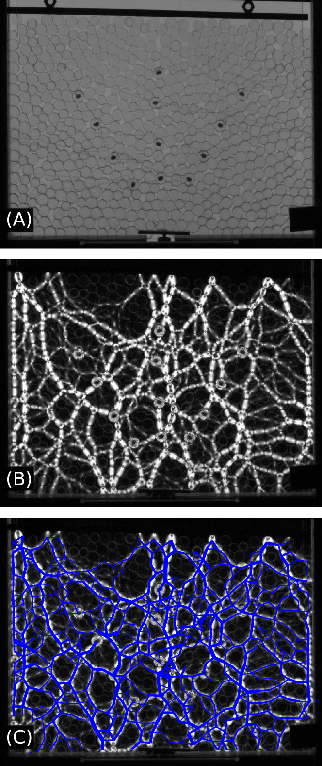
Particulate matter comes in many forms: it ranges from frictionless emulsions and frictional granular materials to bonded composites and biological cells. A long-known hallmark of particulate systems is the heterogeneous distribution of inter-particle forces within them Dantu (1957); Liu et al. (1995); Radjai et al. (1996); Mueth et al. (1998); Howell et al. (1999); Majmudar and Behringer (2005)—a phenomenon that has come to be known as force chains. The term “force chain” arises from the appearance—particularly in two-dimensional (2D) systems—of chains of particles that transfer force from one particle to another along the chain. In Fig. 1, for example, the eye readily focuses on the backbone that arises from the set of bright particles. These particles experience forces that are larger than average, and one can see such forces by using photoelastic particles and placing them between crossed polarizers. In both two and three dimensions, it is increasingly common to measure inter-particle forces in a variety of systems – including frictional grains Majmudar and Behringer (2005); Saadatfar et al. (2012), frictionless grains Mukhopadhyay and Peixinho (2011), and frictionless emulsions Brujić et al. (2003); Zhou et al. (2006); Desmond et al. (2013). This opens the door for achieving a better understanding of force chains in a variety of systems.
It is known that force chains are important for resisting shear Howell et al. (1999) and directing sound propagation Makse et al. (1999); Cruz Hidalgo et al. (2002); Somfai et al. (2005); Owens and Daniels (2011), but little is known about which properties of these chains are universal to particulate systems and which are sensitive to details (such as friction, adhesion, boundary conditions, and body forces like gravity). Improved methods for automatically identifying force chains and quantifying their specific properties (e.g. size and shape) would yield a deeper understanding of how they impact mechanical properties of particulate systems.
Although the presence of force chains is a generic feature of particulate systems, the term “force chain” is often used colloquially, and the field still lacks a quantitative definition of the term. Recently, several techniques have been proposed that aim to identify which subset of particles form a “force-chain network.” Peters et al. Peters et al. (2005) calculated force chains in low friction by demanding two requirements: particles must occur in a “quasi-linear” arrangement, and they must contain a concentrated stress. They used an algorithm that requires a choice of a threshold value for each of the two conditions, and their notion does not allow force chains to branch. Using discrete-element simulations with a flat-punch geometry, Peters et al. Peters et al. (2005) obtained force chains that contain approximately half of the particles in a system. Additionally, they reported that the lengths of these chains satisfy an approximately exponential distribution. Arevalo et al. Arévalo et al. (2010) examined polygonal structures that underly a force-chain network, which they determined by selecting all inter-particle forces above some threshold. In their numerical simulations, they observed that triangular structures dominate the network near a critical packing fraction. More recently, topological tools such as computational homology have been used to address the question of how to determine the structure of force chains Kondic et al. (2012); Kramár et al. (2014); Ardanza-Trevijano et al. (2014). For example, using numerical simulations, Kondic et al. Kondic et al. (2012) were able to distinguish between frictional and frictionless packings via a topological invariant known as the Betti number Edelsbrunner and Harer (2010). They demonstrated that the Betti number changes with packing density, and they used a force threshold to isolate strong forces from weak forces.
The above investigations have been informative, but they also share a common viewpoint that the strongest inter-particle forces form the backbone of a particulate system. However, even a linear chain of strong particles would not be stable against buckling without the participation of the particles that lie alongside them Radjaï et al. (1998). Therefore, it is necessary to develop techniques that do not include a minimum threshold force to be able to consider a particle to be part of a network.
The purpose of the present paper is to use an approach based on network science Newman (2010) to develop an example of an appropriate method. Network science provides a powerful set of tools to represent complex systems by focusing not only on the components of such systems, but also on the interactions among those components. A network representation is particularly appropriate for particulate systems, where particles (network nodes) are connected to one another by contact forces (network edges).
In Fig. 1, we show an example network, which we constructed from laboratory experiments. Network approaches in granular materials have already had several success in describing the dynamics of granular materials. For example, prior studies have investigated spatial patterns in the breaking of edges in a (binary) contact network under shear Herrera et al. (2011); Tordesillas et al. (2010); Walker and Tordesillas (2010); Slotterback et al. (2012) and the influence of network topology on acoustic propagation Bassett et al. (2012). The latter study established the importance of using weighted contact networks to take into account the strength of inter-particle forces. Several other papers have also recently contributed to this line of inquiry using a variety of different network-based approaches Lopez et al. (2013); Arévalo et al. (2013); Walker et al. (2014); Navakas et al. (2014).
In the present paper, we use network representations to build a set of practical methods to (1) automatically extract force chains from force networks (without the use of thresholding) and (2) define a set of three scalar quantities that one can use to characterize and classify different particulate materials. In Section II, we present two commonly-used granular systems (which are rather different from each other) in which it is possible to measure inter-particle forces. These two case studies—one in a “wet” laboratory and the other based on a standard computational model for jammed packings—provide a basis for describing the utility of our new technique. In Section III, we describe our method to automatically extract the force-chain structure from a force network.
Our method uses community detection, which is a form of clustering for networks Porter et al. (2009); Fortunato (2010). In contrast to previous uses of community detection in particulate systems Ronhovde et al. (2011); Bassett et al. (2012), our method incorporates a geographical null model to account for spatial embeddedness. This geographical null model makes it possible to to identify clusters of particles that are more densely interconnected via strong contact forces than expected given their geographical proximity. We then calculate a gap factor that allows one to optimize the resolution at which the detected communities are maximally branched. One can use the gap factor to quantify similarity of a community’s geometry to that expected in a force chain. The gap factor is larger when communities are more branch-like and thus more similar to the expected geometry of a force chain; it is smaller when communities are either more compact or more string-like, and thus less similar to the expected geometry of a force chain. In addition to the gap factor, we use two other diagnostics—size and network force—to help characterize particulate structures. (We define the three diagnostics in Section III.2.) We then apply our methodology to force networks that we measure in two very different case studies. We demonstrate the utility of our diagnostics for (1) quantifying changes in force-chain structure as a function of the confining pressure applied to a granular material and (2) facilitating the comparison and classification of force-chain network architectures across different media. We conclude and discuss several implications of our work in Section V.
II Methods
To better understand which features of force chains are universal and to demonstrate that our methodology for identifying force chains is insightful for particulate systems in general, we compare and contrast results from two very different case studies: granular experiments and frictionless simulations. In both situations, the particles are confined in two dimensions, and they each consist of packings of bidisperse disks that interact with each other in a Hertzian-like manner. Both cases are jammed under constant pressure and use approximately the same number of particles (600). The key differences between the two systems are (1) the presence of friction and gravitational pressure in the experiments and (2) the use of periodic boundary conditions in the simulations. Additional differences include a different fabric tensor due to different initial conditions and the fact that laboratory experiments have a slight fine-scale polydispersity for particles of the “same” size in addition to the coarse-scale bidispersity. For each of the experiments and simulations, we measure force-contact networks for (approximately) the same seven different values of confining pressure.
II.1 Granular Experiments
We perform experiments on a vertical 2D granular system of bidisperse disks that are confined between two sheets of Plexiglas. The particles are mm thick, their diameters are mm and mm (which yields a diameter ratio of approximately 1.22), and they are cut from Vishay PSM-4 photoelastic material to provide measurements of the internal forces. These particles have an elastic modulus of MPa. We produce new configurations by rearranging the particles by hand. We increase the pressure by placing additional brass weights on the top surface of the packing. The values of pressure, which we report in units of the elastic modulus (recall that the configuration is two-dimensional), are , , , , , , and . Particles are constrained by vertical walls to prevent deformation due to these pressures from occurring in the direction perpendicular to the loading direction. Such constraints on deformation can influence the shape of force chains, which tend to form in the direction of the major principal stress Tordesillas et al. (2010); Majmudar and Behringer (2005); Radjai and Azéma (2009). See Refs. Owens and Daniels (2011); Bassett et al. (2012); Owens and Daniels (2013) for additional details about the experiments.
For each of 21 particle configurations and the seven values of pressure, we compute particle positions and forces using two high-resolution pictures of the system. We use one image, which we take without the polarizers, to determine the particle positions and contacts. (See Puckett and Daniels (2013) for a description of the technique.) We take particles to be in contact if the force between them is measurable by our photoelastic calculations. Using a second image that we take with the polarizers, we then determine the particle contact forces by solving the inverse photoelastic problem Puckett and Daniels (2013).
II.2 Frictionless Simulations
We perform numerical simulations of a 50:50 ratio of bidisperse frictionless disks. We use a diameter ratio of , and particles interact via a Hertzian potential in a box with periodic boundary conditions in both directions and zero gravity O’Hern et al. (2002, 2003); Manning and Liu (2011). This model has been well-studied and it is significantly different from our experimental system with respect to friction, gravity, and the fixed boundaries. We generate mechanically-stable packings via a standard conjugate-gradient method O’Hern et al. (2002). We then perform simulations for a fixed packing fraction and volume, and we analyze 20 mechanically-stable packings at each packing fraction . We choose the seven values of the packing fraction so that the mean pressure at that packing fraction 111For finite systems, there isn’t a bijection between pressure and packing fraction. Because the packing fraction is fixed in these simulations, there is some variance (of roughly ) in the pressure between different packings. matches the ones in the experiments: , , , , , , and , where the modulus is defined as the energy scale for the Hertzian interaction divided by the mean Voronoï area of a particle in the packing. The smallest value of provides a data point for a jammed packing that is less dense than what is accessible in our experiments.
III Force-Chain Extraction and Characterization
III.1 Force-Chain Extraction
To locate the force chains, we begin by recording which particles are in contact with (and exert force on) which other particles. In network language, we represent each particle as a node, and we represent each inter-particle contact as an edge whose weight is given by the magnitude of the force at that contact. We thereby construct a force-weighted contact network from a list of all inter-particle forces. If particle and are in contact, then , where is the normal force between them. If two particles are not in contact, then . In addition, we let . We also construct an unweighted (i.e., binary) matrix whose elements are
The matrix is often called an “adjacency matrix” Newman (2010), and the matrix is often called a “weight matrix.”
To obtain force chains from , we want to determine sets of particles for which strong inter-particle forces occur amidst densely connected sets of particles. We can obtain a solution to this problem via “community detection” Porter et al. (2009); Fortunato (2010); Newman (2012), in which we seek sets of densely connected nodes called “modules” or “communities.” A popular way to identify communities in a network is by maximizing a quality function known as modularity with respect to the assignment of particles to sets called “communities.” Modularity is defined as
| (1) |
where node is assigned to community , node is assigned to community , the Kronecker delta if and only if , the quantity is a resolution parameter, and is the expected weight of the edge that connects node and node under a specified null model.
One can use the maximum value of modularity to quantify the quality of a partition of a force network into sets of particles that are more densely interconnected by strong forces than expected under a given null model. The resolution parameter provides a means of probing the organization of inter-particle forces across a range of spatial resolutions. To provide some intuition, we note that a perfectly hexagonal packing with non-uniform forces should still possess a single community for small values of and should consist of a collection of single-particle (i.e., singleton) communities for large values of . At intermediate values of , we expect maximizing modularity to yield a roughly homogeneous assignment of particles into communities of some size (i.e., number of particles) between and the total number of particles. (The exact size depends on the value of .) The strongly inhomogeneous community assignments that we observe in the laboratory and numerical packings (see Section IV) are a direct consequence of the disorder in the packings.
An important choice in maximizing modularity optimization is the null model Newman (2006a); Bassett et al. (2013). The most common null model for modularity optimization is the Newman-Girvan (NG) null model Newman and Girvan (2004); Newman (2006b); Porter et al. (2009); Fortunato (2010)
| (2) |
where is the strength (i.e., weighted degree) of node and . The NG null model is most appropriate for networks in which a connection between any pair of nodes is possible. Importantly, many networks include (explicit or implicit) spatial constraints that exert a strong influence on which edges are present Barthelemy (2011). For particulate systems, numerous edges are simply physically impossible, so it is important to improve upon the NG null model for such applications. We use the term geographical constraints to describe the explicit spatial constraints in such systems. These constraints exert a significant effect on network structure, so it is important to take them into account when choosing a null model. For granular materials (and other particulate systems), each particle can only be in contact (i.e., ) with its immediate neighbors. We therefore use a null model, which we call the geographical null model, to account for this constraint. The geographical null model is
| (3) |
where is the mean edge weight in a network and is the binary adjacency matrix of the network. (Such a null model was used previously for applications in neuroscience Bassett et al. (2013).) Recall that the adjacency matrix encapsulates the presence or absence of contact between each pair of particles. For a granular material, is the mean inter-particle force. Because we have normalized the edge weights in the force network (), we note that in our case .
Maximizing yields a so-called “hard partition” of a network into communities in which the total edge weight inside of modules is as large as possible relative to the chosen null model. A hard partition assigns each node to exactly one community. (An alternative is a “soft partition” Walker and Tordesillas (2014), which allows each node in a network to be associated with multiple communities.) For the geographical null model in (3), maximizing assigns the particles into communities that have inter-module particle forces that are larger than the mean force. Such communities represent the force chains in a granular system.
Because maximizing is NP-hard Brandes et al. (2008), the success of the maximization is subject to the limitations of the employed computational methods. In the present paper, we use a Louvain-like locally greedy algorithm Jutla et al. (2012). Additionally, given the numerous near-degeneracies in the modularity landscape that tends to inflict networks that are constructed from empirical data Good et al. (2010) (i.e., many different partitions often yield comparably large values of ), we report community-detection results that are ensemble averages over 20 optimizations.
III.2 Properties of Force Chains
We characterize communities using several diagnostics: size, network force, and a gap factor (a novel notion that we introduce in the present paper). The size of a community is simply the number of particles in that community. The systemic size is given by the mean of over all communities. The modularity is composed of sums of magnitudes of bond forces and therefore also has units of force. Therefore, we use the term network force to indicate the contribution of a community to modularity. The network force of a community is given by the formula
| (4) |
where is the set of nodes in community . The systemic network force is the mean of over all communities. Communities that correspond to force chains composed of densely packed particles with large forces between them have large values of network force, whereas communities that correspond to force chains composed of sparsely packed particles with small forces between them have small values of network force.
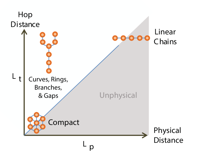
To identify the presence of gaps and the extent of branching in the geometry of a force-chain network, we calculate the Pearson correlation between “physical distance” (which we measure using the standard Euclidean metric) and “hop distance” (which is often called the “topological distance” and counts distance measured only along network edges), and we examine how the correlation depends on the force-chain topology. Communities with compact or linear-chain characteristics (see the main diagonal in Fig. 2) occur when there is a perfect correlation between hop distance and physical distance. The perfect correlation arises because particles that are one hop away from each other (i.e., they are adjacent to each other in the binary contact network) are also 1 particle-distance away. Small linear chains occur close to the origin, where both hop distance and physical distance are small, whereas long linear chains occur in the upper right quadrant of Fig. 2. Note that we use the term “compact” in the spirit of the mathematical sense of the term, although our exact meaning is somewhat different: “compact” communities of particles are at the opposite extreme as linear chains. Small compact blobs contain particles that are 1 hop-distance away from one another and 1 particle-distance away from one another, and they therefore occur near the origin of Fig. 2. Larger compact blobs contain particles that are several hop-distances away (and an equal amount of particle-distances away), and they therefore occur in the upper right quadrant of Fig. 2.
In contrast to compact blobs and linear chains, force chains with gaps, branches, and rings have a larger hop distance than physical distance (see the upper triangle in Fig. 2). Particles that are close together in space do not necessarily have strong forces to bind them; the presence of more complicated shapes decreases the correlation between the physical and hop distance. (Note for particulate systems that the lower triangle is unphysical, as it would require forces between particles that are not in contact with one another to achieve a larger physical distance than hop distance.)
To identify communities that are composed of branched structures, we measure the amount of correlation between the hop distance and the physical distance in the set of all node pairs in a given community. To compute the hop distance of a community, we define the community contact network . Its elements are entries of the matrix for which the corresponding nodes have both been assigned to the same community . We then calculate the path lengths between possible pairs of nodes in a community using the hop distance on the matrix . The resulting matrix of pairwise distances is . To compute physical distance, we calculate the Euclidean distances between all possible pairs of nodes in a community. The resulting matrix of pairwise distances is .
In defining the community gap factor, we choose to weight each community by its size. We thus weight large communities more heavily than small communities in linear proportion to the number of particles that they contain. In this case, the gap factor of a community measures the presence of gaps and the extent of branching in a community. We calculate it using with the formula
| (5) |
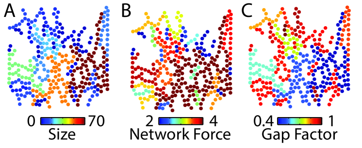
where is the value of the Pearson correlation between the upper triangle of and the upper triangle of , and is the size of the largest community. (Note that we exclude the diagonal elements of the matrices and .) To provide further illustration of this quantity, a set of communities colored by their respective gap-factors is shown in Fig. 3(C).
We define the (weighted) systemic gap factor as
| (6) |
where the quantity is the total number of communities (including singletons) and we again note that large communities contribute more than small communities to the averaging in Eq. (6). An alternative choice for the systemic gap factor is to weight all communities uniformly to calculate an alternative systemic gap factor
| (7) |
As we discuss in more detail in the appendix, branched communities typically include more nodes than linear communities, so the weighted gap factor tends to be larger for communities with more branching. By contrast, tends to be larger for more linear communities. For the remainder of the main manuscript, we focus on the weighted gap factor because it varies far less across packings. Further studies of would also be interesting.
IV Characterizing Force Chains
We now characterize the force-chain networks of the experiments and simulations that we described in Section II using the methodology that we described in Section III. Our community-detection procedure consists of two stages. First, we maximize modularity (1) with the geographical null model (3) for different values of the resolution parameter : from to in increments of . We then choose a resolution that approximately maximizes the systemic gap factor [see Eq. (6)]. This ensures that we extract communities of particles that have strong and dense force-weighted contacts with one another (i.e., our network partition has a large value of the modularity ), and that they are spatially sparse (i.e., they tend to have a small topological-physical distance correlation ). The communities that we obtain tend to take the form of chain-like structures that are reminiscent of force chains; this provides visual support that our technique is successful. Our communities are much better than what one obtains using the NG null model. In previous work using the NG null modelBassett et al. (2012), we observed that these latter communities always tend to be compact in form. We know, however, that communities with other qualitative features are very common. (See the schematic in Fig. 2.)
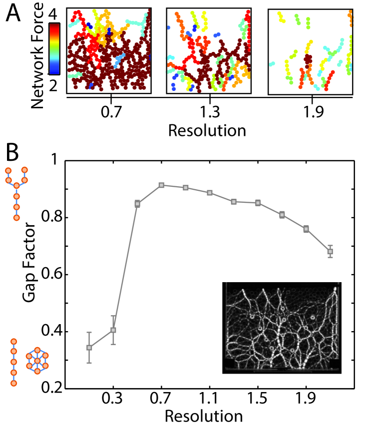
The resolution parameter sets the spatial resolution of the communities Reichardt and Bornholdt (2006); Porter et al. (2009); Onnela et al. (2012) [see Eq. (1)]. By tuning , one can either examine large communities (using small values of ) or small communities (using large values of ). In Fig. 4A, we show an example computation using data from experiments. (Note that we do not show single-particle communities.) Observe that small values of produce communities that are dominated by compact structures ( small ), whereas large values of produce communities that are dominated by linear structures ( small as well). This suggests that we can identify an optimal value that maximizes the systemic gap factor . This also corresponds to the choice for which the detected communities are most similar to the force-chain structure that we observe visually (see Fig. 4B). For this particular packing, we identify as the best choice in our examination of . As one can see in Fig. 4A, we observe at all values of that the detected communities vary in their size, network force, and gap factor. We also note that single-particle communities are common for all values of near 1 (and become increasingly common as increases after it exceeds 1).
Community detection via modularity maximization with a resolution parameter chosen to yield a maximal systemic gap factor provides an automated approach for detecting force chains in granular media. Once identified, we then calculate the size , network force , and gap factor to describe key features of a force-chain network. In the following subsections, we quantitatively examine how the distributions of , , and vary as a function of pressure for both granular experiments and frictionless simulations.
IV.1 Granular Experiments
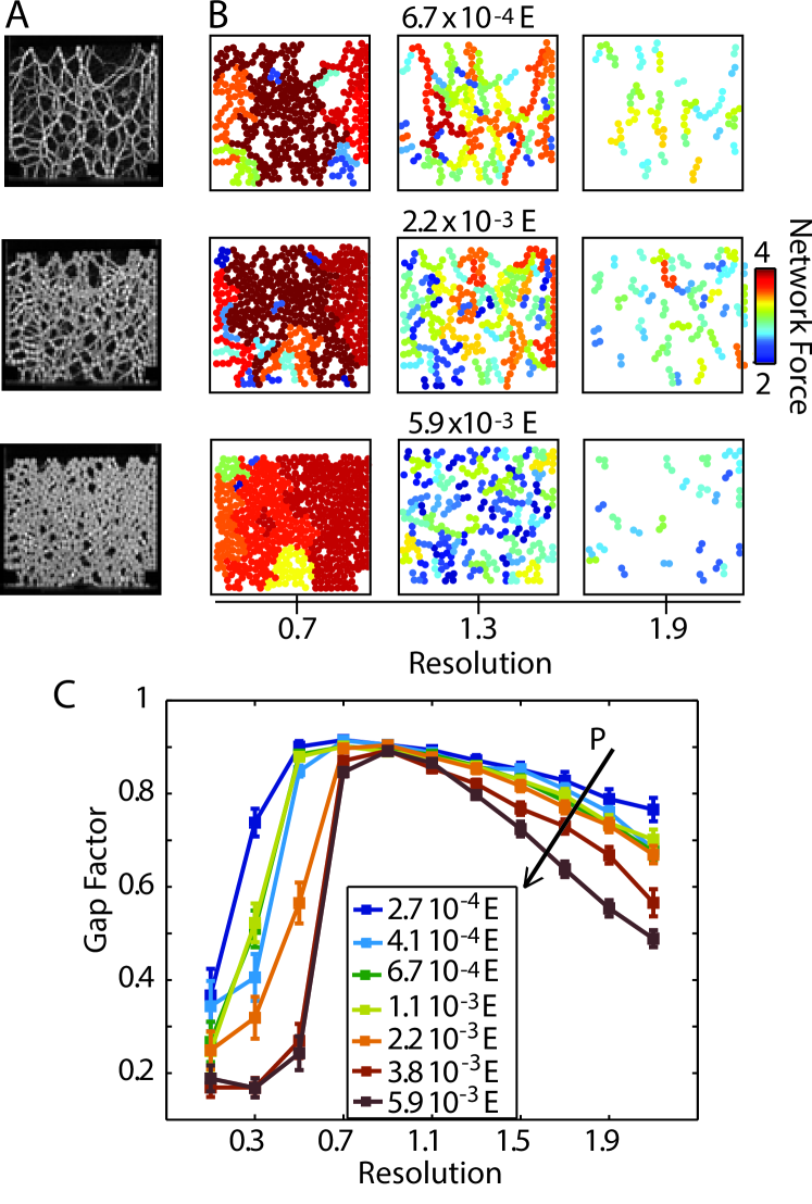
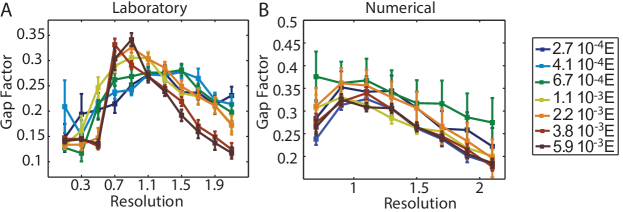
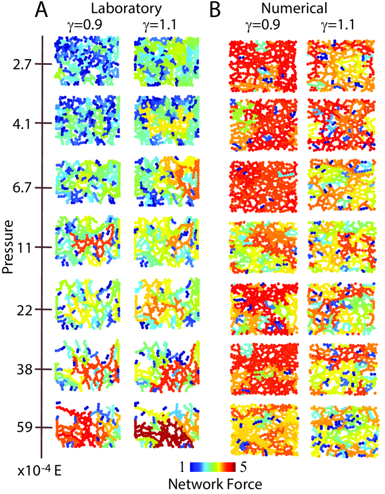
Our experiments are at seven different pressures, which range from to . As we illustrate in Fig. 5A, we observe that the communities become more compact (so they are closer to the diagonal line in Fig. 2) as pressure increases. At a small value of the resolution parameter (), the detected communities metamorphose from branched structures to compact domains as pressure increases. At a large value of the resolution parameter (), the detected communities tend to shrink from many-particle chains to -particle chains as pressure increases. This provides a way to quantify our earlier observations that force-chain networks at higher pressures are more homogeneous (observations at small ) and less chain-like (observations at large ) than they are at lower pressures.
At all pressures (and despite the aforementioned differences), we find a maximum in the systemic gap factor as a function of the resolution parameter (see Fig. 5B). The shape of the curve of the gap factor versus the resolution-parameter has a more pronounced peak at higher pressures than at lower pressures: larger slopes descend from and (especially) lead up to the values of near the maximum. At all pressures, small values of select compact communities and large values of select two-particle communities. In between, we observe a value of at which the most branch-like structures appear; we refer to this value that approximately maximizes the gap factor as the “optimal” value. This optimal value changes slightly as a function of pressure; for example, at and for . High-pressure packings also exhibit a much smaller systemic gap factor than low-pressure packings at both small and large values of the resolution parameter. This observation is consistent with both the increased compactness of the communities and the increasingly homogeneous nature of the force-chain structure as one increases the pressure.
The resolution that maximizes the gap factor identifies structures in a force network that are most reminiscent of the force chains that are apparent by eye; in other words, it identifies branching communities. Therefore, to extract force chains from force networks across different packings and pressures, we examine community structure for a range of resolution parameters and identify the resolution-parameter value that approximately maximizes the gap factor. We refer to the communities detected at as the “force chains” in our calculations, and we characterize their properties in terms of their size, network force, and gap factor. For an illustrative example of a single packing whose communities are color-coded by either size, network force, or gap factor (see Fig. 3).
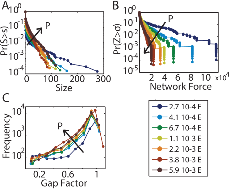
As we illustrate in Fig. 6, we observe that the size and network force of the force chains have approximately exponential distributions for all seven pressures. This identifies that the majority of communities are relatively small and weak, but a few communities are relatively large and strong. By contrast, the gap-factor distribution is skewed: most communities have a large gap factor, and only a few communities have a small gap factor. In high-pressure packings, communities tend to be less broadly distributed with respect to both size and network force; this is consistent with the homogenization of force chains as pressure increases.
IV.2 Frictionless Simulations
To illustrate quantitative differences in force-chain structure between laboratory and numerical packings, we use our methodology to identify force chains in frictionless simulations. In addition to their lack of friction, the numerical packings also differ from our experiments in that they use periodic boundary conditions, have zero gravity, have zero fine-scale polydispersity, and have a different fabric tensor due to their different initial conditions. (A commonality between the two types of packings is that they are both bidisperse.) As in Section IV.1, we find communities via modularity maximization at different values of the resolution parameter for different packing fractions, which we select to match the seven pressures from the experiments.
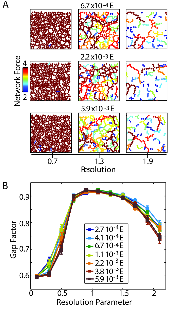
As we show in Fig. 7A, the simulated packings change qualitatively as a function of the resolution parameter. For relatively small values of the resolution parameter (), the granular force network has collapsed into a single compact community. In contrast, for relatively large values of the resolution parameter (), we identify many small branch-like communities that are reminiscent of force chains. Unlike in the granular experiments, we do not observe a strong qualitative change in community structure as a function of pressure (regardless of the value of ). Compare Figs. 5B and 7B.
In order to select the most branched community structure, we again identify a value that is associated with the maximum value of the systemic gap factor . As with the experimental packing, there is a clearly identifiable maximum (see Fig. 7B), which occurs at for . We also observe that the shape of is more consistent across pressures for the simulations than it is for the experiments.
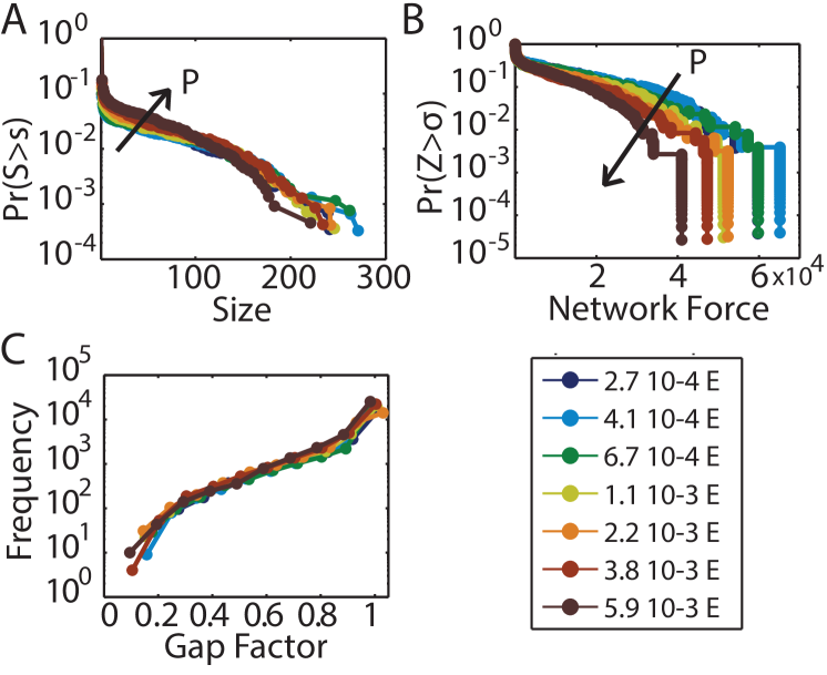
As in the laboratory packings, we refer to the communities at as our “force chains,” and we characterize their properties in terms of size, network force, and gap factor (see Fig. 8). Across the set of pressures from to , we observe that chain size and network force have approximately exponential distributions. This indicates that the majority of communities are relatively small and weak, but a few communities are relatively large and strong. The gap-factor distribution has a left skew, which indicates that most communities have a large gap factor and only a few communities have a small gap factor.
In contrast to the laboratory experiments, the shape of the distributions for size, network force, and gap factor in frictionless simulations do not change dramatically as a function of pressure. Nevertheless, the frictionless simulations to exhibit a systematic difference in the mean size and mean network force for communities as a function of pressure [see Fig. 8B].
IV.3 Comparison Between Laboratory and Numerical Force Chains
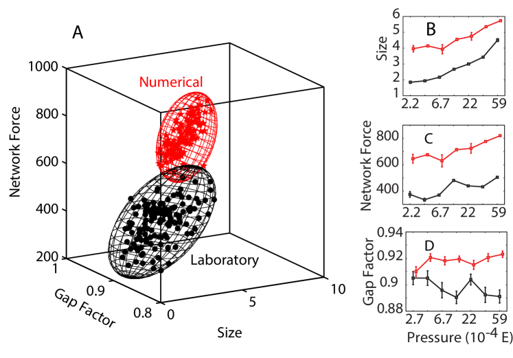
Using our methodology of extracting force chains, it is possible to quantitatively compare and contrast two particulate systems (such the aforementioned granular experiments and frictionless simulations). In Fig. 9, we summarize the three main diagnostics (size, network force, and gap factor) that we calculate for each of our two case studies. We anticipate that these diagnostics might provide a helpful means of characterizing how well a given set of simulations—e.g., with anisotropic cell shapes Mailman et al. (2009); Zeravcic et al. (2009) or different models of friction Cundall and Strack (1979); Papanikolaou et al. (2013)—captures experimental features. It also provides a systematic way to compare the properties of different particulate systems or to monitor the temporal evolution of a particulate system.
The first key difference between our results for the experimental and numerical packings is that the granular experiments have force chains with smaller mean size and network force (compare Figs. 9A and B). This result is consistent with the more homogeneous nature of force chains in the frictionless packings than in the laboratory packings. Laboratory packings exhibit a few large and strong force chains (see Figs. 6A and B), but the majority of a packing tends to be dominated by singleton communities (see Fig. 6A). By contrast, the frictionless packings have community-size and network-force distributions that are far less skewed (see Fig. 8). Additionally, the majority of such a packing is dominated by the force chains (see Fig. 8A); there are few singletons. These differences in the homogeneity of the packings and in the distributions of size and network force leads on average to larger and stronger force chains in the frictionless numerical packings than in the laboratory ones.
We also observe that the gap factor is smaller on average in the laboratory packings than in the frictionless packings. This result is also consistent with the homogenization of structure in frictionless packings, but it might also be influenced by differences between the two types of packings from the presence versus absence of gravity. The frictionless packings are gravity-free, whereas the laboratory packings are influenced by gravity. In contrast to the frictionless packings, the laboratory packings therefore often exhibit linear vertical chains, which decrease the systemic gap factor. (See our discussion in Appendix 2.)
Finally, we observe that the size and network force of chains increases with pressure in laboratory packings, whereas the systemic gap factor decreases with pressure for such packings. These observations indicate the presence of a changing length scale, as is to be expected Wyart et al. (2005); Goodrich et al. (2013). As pressure increases, the force structure becomes more homogeneous, leading to extended sections of material with densely packed particles that exert strong forces on one another. However, the force structure becomes less branch-like, leading to a decrease in the systemic gap factor. The frictionless numerical packings also exhibit increases in size and network force of chains with pressure; however, unlike in the laboratory packings, the frictionless packings do not exhibit a decrease in systemic gap factor with pressure. This quantitative difference between the two types of packings yields a technique for measuring the visual differences between Figs. 5A and 7A, in which it is clear that the geometry of the force chains is affected less by pressure in the simulated setting than in the laboratory setting.
Figure 9B also demonstrates that the size of communities that resemble force chains decreases as pressure approaches , which provides some elucidation for a longstanding question in the field of disordered matter. In particulate systems at temperature, the point at which pressure is the jamming transition, and a lot of recent work has been devoted to attempting to understand the nature of this transition Liu and Nagel (2010). There is now strong evidence that there is a growing length scale Wyart et al. (2005); Goodrich et al. (2013), which corresponds to the size of regions that are mechanically unstable, near the transition. As we discuss in Section V, it is natural to postulate that our force-chain communities are negatively correlated with weak regions in a particulate packing. Therefore, we expect force chains to shrink as mechanically unstable regions grow.
V Conclusions and Discussion
In this paper, we treated granular materials as spatially-embedded networks in which nodes (particles) are connected by edges whose weights we determine from contact forces. We developed and applied a network-based clustering method, in which we detect tightly-connected “communities” of particles via modularity maximization with a geographical null model, to extract chain-like structures that are reminiscent of force chains in both numerical and laboratory packings. From these chain-like structures, we calculated three key diagnostics (size, network force, and gap factor), and we illustrated their utility for identifying and characterizing force-chain network architectures across two types of packings (laboratory and numerical) and across seven different pressures. To characterize force chains, we identified an “optimal” resolution-parameter value that approximately maximizes the gap factor in each of these scenarios. An alternative approach would be to examine the structure of force chains that are identified at a set of resolution parameters that one optimizes separately by considering other parameters (e.g., size, network force, etc.). This is an interesting direction for future study.
After we identified an optimal value for the resolution parameter, we systematically evaluated and compared properties of force-chain communities. A common feature that we observed in both the (frictional) laboratory and (frictionless) numerical packings is that the distribution of force-chain sizes is consistent with an exponential distribution. In the laboratory packings of 2D granular materials, we found that high-pressure force networks exhibit compact rather than branching communities, which is consistent with the notion that increasing pressure causes a breakdown in the long-range heterogeneous structure in a material. In contrast, the geometry of the force chains in the frictionless numerical packings appear to be affected less by pressure. The force chains in the numerical packings also tend to be both larger and stronger than their counterparts in laboratory packings. Together, these results support the conclusion that the force-chain structure, topology, and geometry is different in the two systems.
Methodological Insights
An important conclusion of our paper is that choosing an appropriate null model is critical for extracting information from community detection in networks. We have developed and applied a geographical null model for the detection of network communities, which are strongly reminiscent of force chains, in particulate materials. The power of this null model lies in its ability to fix a network’s topology (which is given by a binary contact network) while scrambling its geometry (which is given by a force-weighted contact network). The geographical null model thereby includes more of the fundamental physics of particulate systems than the Newman-Girvan null model that is commonly used in modularity maximization. An interesting future direction would be to incorporate different physical constraints and principles (e.g., force balance) and to examine the different results that one obtains by including different combinations of relevant physical ideas. A key question in community detection is what is the minimal set of physical ideas—and, more generally, the minimal amount of problem-specific information—that one can include in a null model to get answers that are more insightful than using a one-size-fits-all null model like the Newman-Girvan model.
Practical Utility
We expect that our methodology will provide a framework for understanding which features of force chains are universal versus which are governed by detailed particle-particle or particle-environment interactions. For example, one can use our methodology to provide a quantification of the similarity of force chains between a simulation and a given experiment. It can also provide similar quantifications between two experiments (or two simulations) with different types of particles or boundary conditions. It is also a viable tool to help predict differences in macroscropic behavior based on subtle differences in the mean or distributions of force-chain diagnostics.
Our methodology also provides additional information that is not available via traditional methods for identifying force chains. For example, we know which particles are strongly connected within communities, and we can also observe the spatial arrangement of the various communities that comprise a force network. This allows one to ask whether the arrangement of communities helps to govern the linear and nonlinear response of a disordered packing. For example, it is possible that large, strong communities indicate a region of relatively high mechanical stability or that boundaries between these communities indicate areas of weakness. In the future, these types of investigations should be helpful for obtaining a better understanding of the onset of flow or failure in particulate systems.
Acknowledgements
DSB was supported by the Alfred P. Sloan Foundation, the Army Research Laboratory through contract number W911NF-10-2-0022 from the U.S. Army Research Office, and the National Science Foundation award #BCS-1441502. KED and ETO were supported by NSF-DMR-0644743 and NSF-DMR-1206808, and they thank James Puckett for the development of the photoelastic image-processing code. MLM was supported by the Alfred P. Sloan Foundation, NSF-BMMB-1334611, and NSF-DMR-1352184. MAP was supported by the James S. McDonnell Foundation (research award #220020177), the EPSRC (EP/J001759/1), and the FET-Proactive project PLEXMATH (FP7-ICT-2011-8; grant #317614) funded by the European Commission. The content is solely the responsibility of the authors and does not necessarily represent the official views of the funding agencies.
Appendix 1: Effect of Community Weighting on Force-Chain Extraction
In this appendix, we describe an alternative set of measurements that we make using the uniformly-weighted systemic gap factor , which we defined in Eq. (7).
Gap Factor Versus Resolution Parameter
In Fig. 10, we observe that the curve of the maximum of versus the resolution parameter varies significantly with pressure in the (frictional) laboratory packings but not in the (frictionless) numerical packings. In the laboratory packings, we observe a maximum of at (for ) in high-pressure packings ( E) and at for low-pressure packings ( E). In the numerical packings, we observe a maximum of at for all pressures. In comparison to our observations in the main text from employing the size-weighted systemic gap factor , we find that the optimal value of is larger when we instead employ (compare Fig. 10 to Fig. 5 and Fig. 7). We also observe that the curves of the systemic gap factor versus resolution parameter exhibit larger variation for the uniformly-weighted gap factor than for the size-weighted gap factor.
Optimal Value of the Resolution Parameter
The large variation in the maximum of over packings and pressures makes it difficult to choose an optimal resolution-parameter value. We choose to take because (1) it corresponds to the maximum of in the numerical packings and (2) it corresponds to the mean of the maximum of in the laboratory packings. To facilitate the comparison of optimal values of from the two weighting schemes, we denote for as and we denote for as . Note that differs from (and is larger than) .
Force-Chain Structure at the Optimal Value of the Resolution Parameter
The force chains that we identify for the optimal value for the uniformly-weighted gap factor (at ) differ from those that we identified in the main text for the optimal value of the size-weighted gap factor (at ). We show our comparison in Fig. 11. For both laboratory and numerical packings, the force chains that we identify at are larger and more branched than the ones that we identify at (which are smaller and more linear). Indeed, the communities that we identify at have more singletons than the communities that we identify at . These results follow from the difference in the two weighting schemes for calculating a systemic gap factor. The size-weighted systemic gap factor weights larger communities more heavily than smaller ones, and the larger communities tend to be the more branched communities that we identify at smaller values of the resolution parameter (e.g., at ). In contrast, the uniformly-weighted systemic gap factor gives equal weight to small and large communities, and it therefore uncovers the linear communities that are evident at larger values of the resolution parameter (e.g., at ). We can therefore use the size-weighted gap factor to identify larger, more branched force chains and the uniformly-weighted gap factor to identify smaller, more linear force chains.
Appendix 2: Methodological Considerations
Robustness of Community Structure to Errors in the Estimation of Contact Forces
In our frictional laboratory experiments, we estimate that errors in the force measurements could be as large as of the contact force ; the high variability arises from the nonlinear fitting process. (Recall that we take particles to be in contact if the force between them is measurable by our photoelastic calculations. We then determine the particle contact forces by solving the inverse photoelastic problem using images taken with polarizers Puckett and Daniels (2013).) Somewhat surprisingly, we find that the errors in the force estimates are independent of both the local force and the global pressure. To ensure that our results are qualitatively robust to these variations, we construct 20 simulated force networks for each experimental network (21 packings, seven pressures) by adding Gaussian noise with width a to each contact. For each of these simulated networks, we reevaluate the estimated community structure (from which we infer the force chains).
To determine whether the estimates are robust to this amount of noise, we compare the community structure of the actual force networks with those of the simulated force networks using the z-score of the Rand coefficient Traud et al. (2011). For comparing two partitions and , we calculate the Rand z-score in terms of the network’s total number of pairs of nodes, the number of pairs that are in the same community in partition , the number of pairs that are in the same community in partition , and the number of pairs that are assigned to the same community both in partition and in partition . The z-score of the Rand coefficient comparing these two partitions is
| (8) |
where is the standard deviation of (as in Traud et al. (2011)). Let the mean partition similarity denote the mean value of over all possible partition pairs for .
We observe that the assignment of particles to communities (and consequently to force chains) in the experimental laboratory force networks is, on average, statistically similar (the z-scores for similarity are larger than 18) to the assignment of particles to communities in the simulated networks constructed by adding Gaussian noise with width to each contact (see Fig. 12A). These results indicate that our estimates of network communities is relatively robust to the empirical measurement error in the inter-particle contact forces.
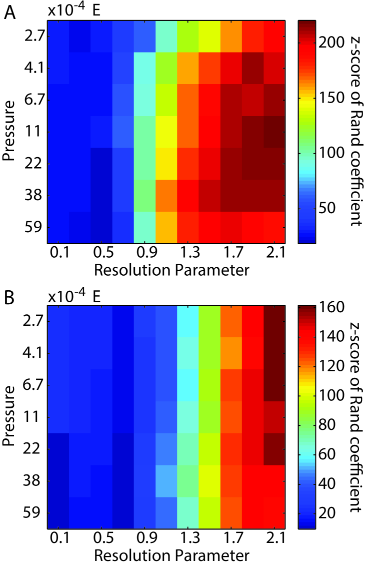
To further clarify the robustness of our algorithm to variations in inter-particle forces on the order of of the contact forces, we perform similar calculations for the numerical packings. For each numerical packing, we construct 20 simulated force networks by adding Gaussian noise with width to each contact. For each of these simulated networks, we reevaluate the estimated community structure (from which we infer the force chains). We observe that the assignment of particles to communities (and consequently to force chains) in the numerical force networks is, on average, statistically similar (the z-scores for similarity are larger than 9) to the assignment of particles to communities in the simulated networks constructed by adding Gaussian noise with width to each contact (see Fig. 12B). These results indicate that our estimates of network communities is relatively robust to measurement error in the inter-particle contact forces in the form of of the contact force.
Effects of Gravity on Community Structure in Laboratory Packings
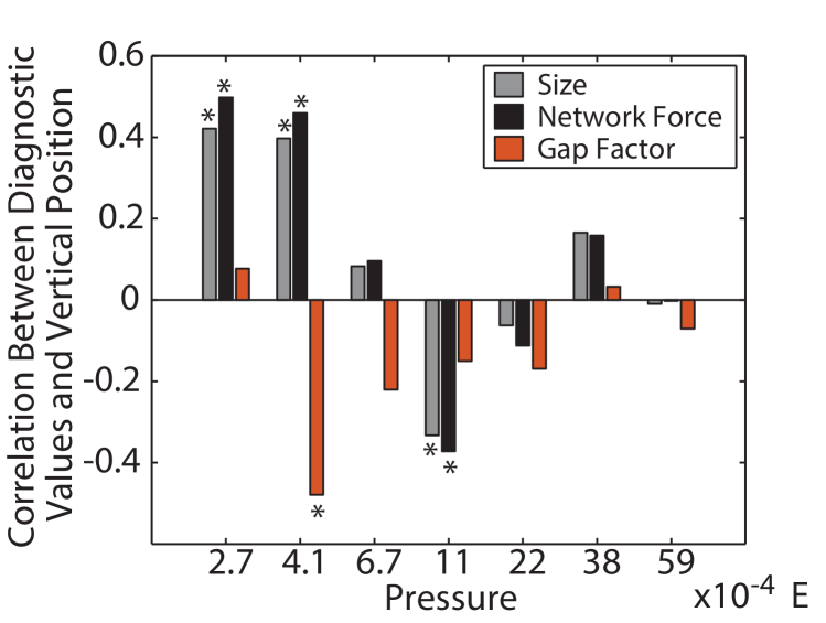
In the laboratory packings, gravity can play an important role in the heterogeneity of observed force chains. To determine the impact of gravity on network diagnostics, we calculate the mean vertical position of particles in each network community for each packing, pressure, and optimization of the modularity quality function for the resolution-parameter value () that maximizes the gap factor. For each pressure value separately, we collate these four diagnostics (size, network force, gap factor, and mean vertical position) for every community that we identify over packings and modularity optimizations. To decrease the potential for false positives, we then identify the unique community sizes, and average network force, gap factor, and mean vertical position over all communities of that size. This process serves as a data-reduction procedure. It decreases the degrees of freedom in subsequent statistical testing, and it thereby decreases the potential for false positives. We then ask whether the network diagnostics (size, network force, or gap factor) are significantly correlated with the mean vertical position of the communities. We use a Spearman rank correlation to increase our robustness to outliers in the data. For low values of pressure we observe a significant correlation between each of the three community-level network diagnostics (size, gap factor, and strength) and the mean vertical position of the particles in that community (see Fig. 13).
At pressures of E and E, larger communities with larger network force tend to be identified at a lower vertical position of the packing; this is consistent with the compaction effects of gravity. At pressures of E, communities with large gap factors tend to be observed at high vertical positions in the packings (where communities tend to be small and less compact). For values of pressure between E and E, we observe no relationship between mean vertical position of particles in a community and community size, network force, or gap factor. These results indicate that gravity can play a role in the shape of force chains, particularly at low pressures.
References
- Dantu (1957) P. Dantu, in Proceedings of the fourth International Conference on Soil Mechanics and Foundation Engineering, London (1957) pp. 144–148.
- Liu et al. (1995) C. H. Liu, S. R. Nagel, D. A. Schecter, S. N. Coppersmith, S. Majumdar, O. Narayan, and T. A. Witten, Science 269, 513 (1995).
- Radjai et al. (1996) F. Radjai, M. Jean, J. J. Moreau, and S. Roux, Physical Review Letters 77, 274 (1996).
- Mueth et al. (1998) D. M. Mueth, H. M. Jaeger, and S. R. Nagel, Physical Review E 57, 3164 (1998).
- Howell et al. (1999) D. Howell, R. P. Behringer, and C. Veje, Physical Review Letters 82, 5241 (1999).
- Majmudar and Behringer (2005) T. S. Majmudar and R. P. Behringer, Nature 435, 1079 (2005).
- Saadatfar et al. (2012) M. Saadatfar, A. P. Sheppard, T. J. Senden, and A. J. Kabla, Journal of the Mechanics and Physics of Solids 60, 55 (2012).
- Mukhopadhyay and Peixinho (2011) S. Mukhopadhyay and J. Peixinho, Physical Review E 84, 2 (2011).
- Brujić et al. (2003) J. Brujić, S. F. Edwards, D. V. Grinev, I. Hopkinson, D. Brujić, and H. A. Makse, Faraday Discussions 123, 207 (2003).
- Zhou et al. (2006) J. Zhou, S. Long, Q. Wang, and A. D. Dinsmore, Science 312, 1631 (2006).
- Desmond et al. (2013) K. W. Desmond, P. J. Young, D. Chen, and E. R. Weeks, Soft Matter 9, 3424 (2013).
- Barthelemy (2011) M. Barthelemy, Phys Rep 499, 1 (2011).
- Makse et al. (1999) H. A. Makse, N. Gland, D. L. Johnson, and L. M. Schwartz, Physical Review Letters 83, 5070 (1999).
- Cruz Hidalgo et al. (2002) R. Cruz Hidalgo, C. U. Grosse, F. Kun, H. W. Reinhardt, and H. J. Herrmann, Physical Review Letters 89, 205501 (2002).
- Somfai et al. (2005) E. Somfai, J.-N. Roux, J. H. Snoeijer, M. van Hecke, and W. van Saarloos, Phys Rev E 72, 021301 (2005).
- Owens and Daniels (2011) E. T. Owens and K. E. Daniels, Europhysics Letters 94, 54005 (2011).
- Peters et al. (2005) J. Peters, M. Muthuswamy, J. Wibowo, and A. Tordesillas, Physical Review E 72, 041307 (2005).
- Arévalo et al. (2010) R. Arévalo, I. Zuriguel, and D. Maza, Physical Review E 81, 041302 (2010).
- Kondic et al. (2012) L. Kondic, A. Goullet, C. S. O’Hern, M. Kramár, K. Mischaikow, and R. P. Behringer, Europhysics Letters 97, 54001 (2012).
- Kramár et al. (2014) M. Kramár, A. Goullet, L. Kondic, and K. Mischaikow, Physical Review E 90, 052203 (2014).
- Ardanza-Trevijano et al. (2014) S. Ardanza-Trevijano, I. Zuriguel, R. Arévalo, and D. Maza, Phys. Rev. E 89, 052212 (2014).
- Edelsbrunner and Harer (2010) H. Edelsbrunner and J. Harer, Computational Topology: An Introduction (American Mathematical Society, 2010).
- Radjaï et al. (1998) F. Radjaï, D. E. Wolf, M. Jean, and J. J. Moreau, Physical Review Letters 80, 61 (1998).
- Newman (2010) M. E. J. Newman, Networks: An Introduction (Oxford University Press, 2010).
- Herrera et al. (2011) M. Herrera, S. McCarthy, S. Slotterback, E. Cephas, W. Losert, and M. Girvan, Physical Review E 83, 1 (2011).
- Tordesillas et al. (2010) A. Tordesillas, D. M. Walker, and Q. Lin, Physical Review E 81, 011302 (2010).
- Walker and Tordesillas (2010) D. M. Walker and A. Tordesillas, International Journal Of Solids And Structures 47, 624 (2010).
- Slotterback et al. (2012) S. Slotterback, M. Mailman, K. Ronaszegi, M. van Hecke, M. Girvan, and W. Losert, Phys Rev E 85, 021309 (2012).
- Bassett et al. (2012) D. S. Bassett, E. T. Owens, K. E. Daniels, and M. A. Porter, Phys Rev E 86, 041306 (2012).
- Lopez et al. (2013) J. H. Lopez, L. Cao, and J. M. Schwarz, Phys. Rev. E 88, 062130 (2013).
- Arévalo et al. (2013) R. Arévalo, L. A. Pugnaloni, D. Maza, and I. Zurigel, Philosophical Magazine 93, 4078 (2013).
- Walker et al. (2014) D. M. Walker, A. Tordesillas, M. Small, R. P. Behringer, and C. K. Tse, Chaos 24, 013132 (2014).
- Navakas et al. (2014) R. Navakas, A. Džiugys, and B. Peters, Physica A: Statistical Mechanics and its Applications 407, 312 (2014).
- Porter et al. (2009) M. A. Porter, J.-P. Onnela, and P. J. Mucha, Not Amer Math Soc 56, 1082 (2009).
- Fortunato (2010) S. Fortunato, Phys Rep 486, 75 (2010).
- Ronhovde et al. (2011) P. Ronhovde, S. Chakrabarty, D. Hu, M. Sahu, K. K. Sahu, K. F. Kelton, N. A. Mauro, and Z. Nussinov, The European Physical Journal E 34, 105 (2011), 10.1140/epje/i2011-11105-9.
- Radjai and Azéma (2009) F. Radjai and E. Azéma, European Journal of Environmental and Civil Engineering 13, 203 (2009).
- Owens and Daniels (2013) E. T. Owens and K. E. Daniels, Soft Matter 9, 1214 (2013).
- Puckett and Daniels (2013) J. G. Puckett and K. E. Daniels, Physical Review Letters 110, 058001 (2013).
- O’Hern et al. (2002) C. O’Hern, S. Langer, A. Liu, and S. Nagel, Phys. Rev. Lett. 88, 075507 (2002).
- O’Hern et al. (2003) C. S. O’Hern, L. E. Silbert, A. J. Liu, and S. R. Nagel, Physical Review E 68, 011306 (2003).
- Manning and Liu (2011) M. L. Manning and A. J. Liu, Physical Review Letters 107, 108302 (2011).
- Note (1) For finite systems, there isn’t a bijection between pressure and packing fraction. Because the packing fraction is fixed in these simulations, there is some variance (of roughly ) in the pressure between different packings.
- Newman (2012) M. E. J. Newman, Nat Phys 8, 25 (2012).
- Newman (2006a) M. E. J. Newman, Physical Review E 74, 036104 (2006a).
- Bassett et al. (2013) D. S. Bassett, M. A. Porter, N. F. Wymbs, S. T. Grafton, J. M. Carlson, and P. J. Mucha, Chaos 23, 013142 (2013).
- Newman and Girvan (2004) M. E. J. Newman and M. Girvan, Phys Rev E 69, 026113 (2004).
- Newman (2006b) M. E. J. Newman, Proc Natl Acad Sci USA 103, 8577 (2006b).
- Walker and Tordesillas (2014) D. M. Walker and A. Tordesillas, in 2014 IEEE International Symposium on Circuits and Systems (ISCAS), Vol. June (2014) pp. 1275–1278.
- Brandes et al. (2008) U. Brandes, D. Delling, M. Gaertler, R. Görke, M. Hoefer, Z. Nikoloski, and D. Wagner, IEEE Trans on Knowl Data Eng 20, 172 (2008).
- Jutla et al. (2012) I. S. Jutla, L. G. S. Jeub, and P. J. Mucha, “A generalized Louvain method for community detection implemented in MATLAB,” (2011–2012).
- Good et al. (2010) B. H. Good, Y. A. de Montjoye, and A. Clauset, Phys Rev E 81, 046106 (2010).
- Reichardt and Bornholdt (2006) J. Reichardt and S. Bornholdt, Phys Rev E 74, 016110 (2006).
- Onnela et al. (2012) J.-P. Onnela, D. J. Fenn, S. Reid, M. A. Porter, P. J. Mucha, M. D. Fricker, and N. S. Jones, Phys Rev E 86, 036104 (2012).
- Mailman et al. (2009) M. Mailman, C. F. Schreck, C. S. O’Hern, and B. Chakraborty, Physical review letters 102, 255501 (2009).
- Zeravcic et al. (2009) Z. Zeravcic, N. Xu, A. J. Liu, S. R. Nagel, and W. van Saarloos, Europhysics Letters 87, 26001 (2009).
- Cundall and Strack (1979) P. A. Cundall and O. D. L. Strack, Geotechnique 29, 47 (1979).
- Papanikolaou et al. (2013) S. Papanikolaou, C. S. O’Hern, and M. D. Shattuck, Physical review letters 110, 198002 (2013).
- Wyart et al. (2005) M. Wyart, L. Silbert, S. Nagel, and T. Witten, Phys Rev E 72, 051306 (2005).
- Goodrich et al. (2013) C. P. Goodrich, W. G. Ellenbroek, and A. J. Liu, Soft Matter 9, 10993 (2013).
- Liu and Nagel (2010) A. J. Liu and S. R. Nagel, Annual Review of Condensed Matter Physics 1, 347 (2010).
- Traud et al. (2011) A. L. Traud, E. D. Kelsic, P. J. Mucha, and M. A. Porter, SIAM Rev 53, 526 (2011).