The Random Walk of High Frequency Trading

Abstract

This paper builds a model of high-frequency equity returns by separately modeling the dynamics of trade-time returns and trade arrivals. Our main contributions are threefold. First, we characterize the distributional behavior of high-frequency asset returns both in ordinary clock time and in trade time. We show that when controlling for pre-scheduled market news events, trade-time returns of the highly liquid near-month E-mini S&P 500 futures contract are well characterized by a Gaussian distribution at very fine time scales. Second, we develop a structured and parsimonious model of clock-time returns by subordinating a trade-time Gaussian distribution with a trade arrival process that is associated with a modified Markov-Switching Multifractal Duration (MSMD) model. This model provides an excellent characterization of high-frequency inter-trade durations. Over-dispersion in this distribution of inter-trade durations leads to leptokurtosis and volatility clustering in clock-time returns, even when trade-time returns are Gaussian. Finally, we use our model to extrapolate the empirical relationship between trade rate and volatility in an effort to understand conditions of market failure. Our model suggests that the 1,200 km physical separation of financial markets in Chicago and New York/New Jersey provides a natural ceiling on systemic volatility and may contribute to market stability during periods of extremely heavy trading.

Keywords: High-frequency trading, US Equities, News arrival.
JEL Classification: C22, C41, C58, G12, G14, G17.

1 Introduction

Modern electronic exchanges function in a manner that outwardly display the properties that are expected of an efficient, liquid market. Bid-offer spreads are narrow in comparison to the price of the underlying instrument being traded, volumes are high, high-frequency traders compete to make markets, and information regarding price discovery is disseminated at nearly the speed of light (see, e.g. Brogaard et al. (2013) and Hasbrouck and Saar (2013)). Within such an environment, the disparate, shifting spectrum of intentions of a wide range of market participants is continuously being aggregated, and so a naive, but nonetheless reasonable, expectation is that the Central Limit Theorem should play a fundamental role, and that short-period returns should adhere to a Gaussian distribution.

Indeed, from the pioneering work of Bachelier (1900) through the development of the Black-Scholes options pricing model (Black and Scholes (1973)), modern finance has traditionally held that market price movements can be approximated to a somewhat useful degree by a Gaussian random walk. This concept draws reinforcement from the Efficient Market Hypothesis (Fama (1965)), since the arrival of news shifts the market in an unpredictable manner (Hasbrouck (2003)).

In reality, observed distributions of market returns are markedly non-Gaussian. Regardless of venue and asset class, returns distributions invariably have fat tails, and display the phenomenon of volatility clustering. A rich literature exists which describes both the characterization and the modeling of the observed departures from normality (for a review, see Bouchaud (2005)).

In this contribution, we carry out a ground-level re-examination of the process that generates short-period market returns within the context of high-frequency trading (over time scales ranging from milliseconds to minutes). We analyze three complete months of recent, millisecond-resolution tick data from the extremely liquid near-month E-mini S&P 500 futures contract traded at the Chicago Mercantile Exchange.

Our analysis begins with two basic empirical conclusions. First, we find that asset returns are effectively organized into two groups with distinct properties: those that are the result of trade within a 1,000 second window following pre-scheduled news announcements (referred to as the “active” period), and those occurring at all other times (referred to as the “passive” period). Our analysis shows that conditional on this sorting mechanism, returns distributions exhibit very different tail characteristics as well as patterns of volatility persistence. We suggest that this is attributable to the shocks of pre-scheduled news announcements entering the market.

Second, we demonstrate that high-frequency returns in passive-market periods are well described by a Gaussian distribution when trade time is employed. Brada et al. (1966) introduced the notion of trade time to show that asset returns distributions are nearly Gaussian if the returns process is subordinated with successive transactions (trades) acting as the subordinator. Mandelbrot and Taylor (1967) showed that a Gaussian random walk composed with a subordinating trade-time process is fully consistent with a fat-tailed, Lévy-stable distribution, as suggested in Mandelbrot (1963). Clark (1973) used an alternative subordinator, time measured by volume of transactions, to obtain similar results. More recently, Ane and Geman (2000) show that coarsely sampled intra-day returns also conform to a Gaussian distribution when measured in trade (transaction) time.

Our analysis demonstrates that the Gaussianity of trade-time returns does not immediately extend to high-frequency intra-day returns. That is, high-frequency, trade-time returns exhibit heavy tails and volatility clustering when considered unconditionally throughout the day. However, by excluding the periods surrounding pre-scheduled news events, we confirm the existence of trade-time Gaussianity as well as a lack of volatility persistence.

Building on the empirical observations above, our paper makes two theoretical contributions. First, we develop a model for high-frequency inter-trade durations by expanding the Markov-Switching Multifractal Duration (MSMD) model of Chen et al. (2013). The MSMD model builds on the seminal work of Mandelbrot et al. (1997), Calvet et al. (1997) and Fisher et al. (1997), as well as subsequent work by Calvet and Fisher (2001), Calvet and Fisher (2002) and Calvet (2004). It suggests a parsimonious model of inter-trade durations that has a well-founded physical interpretation and which has been shown to fit historical data well. Since the MSMD model is unable to explain certain features of high-frequency inter-trade durations, we modify the model by composing an MSMD process with waiting times drawn from an Exponential distribution that is chosen so that its maximal expected duration matches the maximal value observed in our sample. Intuitively, this process describes an environment with two types of traders: the majority type, which typically trades quickly and with infrequent pauses (e.g. algorithmic traders), and a minority type which places few orders, spaced by more moderate durations (institutional investors). The resulting Truncated Markov-Switching Multifractal Duration (TMSMD) model does a better job of fitting the empirical density of high-frequency inter-trade durations as well as capturing the strong autocorrelation of volatility.

The second theoretical innovation of our paper is that we couple a trade-time Gaussian random walk with the TMSMD process above to characterize the distribution of asset returns in clock time. In particular, we demonstrate that the subordinating transformation between clock time and trade time for our data can be effectively explained using the the TMSMD model. In this dimension our work differs substantially from that of Ane and Geman (2000): where they begin with a nonparametric estimate of the distribution of clock-time asset returns and work backwards to implicitly define the nonparametric density of trades that would be consistent with trade-time Gaussianity, we work forwards by first compounding a parametric distribution of trade-time returns with a parametric model of duration times (and hence, an associated trade arrival process) to characterize the distribution of clock-time returns. Our contribution is significant because it promotes a structured and parsimonious approach to approximating the observed evolution of asset returns.

Finally, we use our hierarchical model of clock-time returns to fit and extrapolate the empirical relationship between inter-trade duration (alternatively, trade rate) and market volatility. Our model is suggestive of conditions under which trade rate could induce unprecedentedly high levels of volatility and potential market failure. We highlight how this could occur in the presence of market pressures and uncoordinated limit rules among diverse exchanges.

Our paper proceeds as follows. We begin by describing our data in Section 2 and provide an analysis of the distributional characteristics of the data during active and passive subperiods in Section 3. In Section 4, we describe a compound multifractal model of asset returns in clock time which composes a Gaussian model of trade-time returns with a modification of the MSMD model of Chen et al. (2013). Section 5 estimates the model and compares Monte Carlo simulations with observed data. Section 6 extrapolates the model to draw conclusions regarding market behavior during periods of extremely high volatility. Section 7 concludes.

2 Data

In this paper we focus our analysis exclusively on the Chicago Mercantile Exchange (CME) near-month E-mini S&P 500 Futures contract (commodity ticker symbol ES). Although the CME provides a variety of E-mini products, the E-mini S&P 500 futures contract is the most heavily traded, and for this reason it is commonly referred to as the E-mini. As indicated by its name, the E-mini is a futures contract on the value of the S&P 500 index, with a notional value of 50 times the index. We obtained the full record of tick-by-tick trades for the period 18 May 2013 to 18 August 2013 by parsing the CME historical files, encoded in FIX format, which we use to estimate and evaluate our model in Section 4 and 5. We also obtained similar data for the 27-month period spanned by 27 April 2010 to 17 August 2012, which is used in the out-of-sample analysis reported in Section 6.

Despite the fact that the E-mini is a futures contract that does not trade on equities exchanges, its statistical behavior characterizes the dynamics of the equity markets as a whole. This is attributed to its liquidity and the relationship of price formation and information transmission between the futures and equities exchanges in Illinois and New Jersey, as studied in Laughlin et al. (2014).

E-mini futures trade Monday through Friday, starting at 5:00 p.m. Central Time on the previous day and ending at 4:15 p.m., with an additional daily maintenance trading halt from 3:15 p.m. to 3:30 p.m., Central Time. We aggregate multiple trades occurring within single milliseconds as unit transactions and assign to them the final, in-force price of the millisecond as the price of the trade. While not a perfect approximation, this assumption exploits the fact that multiple transactions with the same time stamp are often attributable to a single aggressor order filling several resting orders at the same price level and also allows us to circumvent singularities associated with zero durations in our subsequent models. Our resulting data for the sample period contains a total of 6,832,305 such transactions.

The quoted price of the E-mini corresponds to the index value of the S&P 500. Since the S&P 500 is an index and not a traded asset, its value is measured in “points” rather than dollars, and as a result E-mini prices are denoted by “points”. The minimum tick increment in the quoted price of the E-mini is 0.25 points, which is the smallest amount by which the E-mini price can change (up or down). In reality, the minimum E-mini contract size is $50 $\times$ the value of the S&P 500, which means that the actual traded price is $50 times the quoted price, with a corresponding minimum increment of $12.50. For the remainder of the paper we will use quoted E-mini prices, measured in points, which correspond directly to the S&P 500 index value. During May through August of 2013, the S&P 500 Index traded between $P=1570$ and $P=1710$, indicating a typical minimum fractional increment in the index price of $\Delta P/P\sim 1.5\times 10^{-4}$.

Because we are interested in investigating the distributions of intra-day asset returns during news event periods and non-event periods, we consider subsamples of the data that sort according to news events. Since the E-mini is a futures contract on a market aggregate, it is almost exclusively affected by major macroecnomic announcements, and not by smaller scale, industry- or firm-specific news. For this reason, we classify news events periods with the EconoDay calendar (econoday.com), which lists major pre-scheduled news announcements in the U.S. and which powers calendars for outlets such as the Wall Street Journal. Since the majority of pre-scheduled news announcements are made at 8:30 a.m. and 10:00 a.m. we form an event-driven dataset of all E-mini trades that occurred during a 1000-second (roughly 16-minute) window following a news announcement at those times. That is, the event-driven dataset is comprised of trades from approximately 8:30-8:46 a.m. and 10:00-10:16 a.m. that follow any pre-scheduled news announcement during the sample period. We form a corresponding non-event-driven subsample that constitutes all trades during the same time windows on days when announcements were not scheduled. A 1000-second window encompasses participants ranging from the fastest algorithmic traders to human traders who manually read the news, consider its implications, and trade on their resulting conclusions.

For the remainder of the paper, we will refer to the event-driven subsample as the active data and the non-event subsample as the passive data. Despite the fact that trading is much heavier during the time windows of the active data, only about 45% of the time windows coincide with scheduled news announcements: there are a total of 43 news periods and 54 non-news periods over the three-month sample. As a result, the two datasets are roughly equal in size: 191,127 records in the active data and 174,041 records in the passive data. Hence, our results below are not an artifact of clock time (both data sets are drawn from the same intra-day time periods) or sample size.

Figure 1 depicts sample paths of E-mini prices during both active and passive periods of our data set. In Figure 1, and for the remainder of the paper, we use red to signify active-period data and blue to signify passive-period data. The upper left panel of the figure shows price series for the 1000 second period following 10:00 a.m. on all days in our sample with a news announcement at that time. These constitute 11 of the 43 news event windows; the remaining 32 news announcements occurred at 8:30 a.m. The prices are sampled at 10-second increments and are normalized by their initial price so that each series begins at the origin. The shading and texture of the individual series are related to the the degree by which the actual announcement differed from a prior consensus forecast. Solid lines indicate announcements that exceeded the consensus and dotted lines fell short. In addition, we sorted the data according to percentage deviation from the consensus, using darker colors to indicate stronger performance and lighter colors to indicate weaker. The legend briefly describes the date and nature of each announcement, along with the prior consensus and actual reported values. As an example, the 10:00 a.m. announcement on 23 May 2013 reported new home sales in the U.S. for the month of April. The prior forecast was that 425,000 units were sold and the actual reported value was 454,000 units – a 6.8% deviation in excess of the consensus.

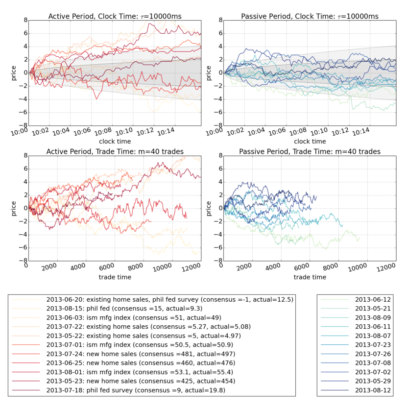
Figure 1: Time series plots of E-mini S&P 500 futures contract prices for the 1000 seconds following 10:00 a.m. news announcements (red) and the 1000 seconds following 10:00 a.m. for a random selection of days without announcements (blue). Prices are all normalized by subtracting the initial price from all subsequent values. The upper panels show clock-time prices while the lower panels show trade-time prices. The legend reports selection dates and information on the individual news announcements. The shaded regions in the upper panels depict expected $1-\sigma$ Brownian motion diffusion bounds on the S&P 500, obtained by deannualizing Gaussian volatilities of $\sigma$=0.1 (inner envelope) and $\sigma$=0.2 (outer envelope).

The upper right panel of Figure 1 shows similar time series for a random selection of 11 days on which there was no 10:00 a.m. news announcement. The figure legend reports the chosen days. In this case, shading sorts series according to the magnitude of return at the end of the 1000 second sample, with darker colors indicating larger returns and lighter colors indicating smaller returns.

The lower panels of Figure 1 replicate the time series of the upper panels, but aggregate prices according to trade time rather than clock time. As we will formalize in the next section, trade time measures time increments according to a specific number of trades occurring rather than a specific amount of wall-clock time elapsing. In this case, we choose $m=40$, meaning that each unit of time is defined by 40 trades, and the resulting trade-time series depict the prices sampled at that frequency.

Two features of the plots are worth highlighting briefly, although we will address them in more detail in the remainder of the paper. First, price movements, relative to their starting points, are much more volatile in the active periods than in the passive periods. The shaded regions in the upper panels of Figure 1 depict expected $1-\sigma$ Brownian motion diffusion bounds on the S&P 500, obtained by deannualizing Gaussian volatilities of $\sigma$=0.1 (inner envelope) and $\sigma$=0.2 (outer envelope). We note that these volatilities can be very roughly equated to values for the CBOE Volatility (VIX) Index of 10 and 20 respectively, which approximately bounded the U.S. equity market during the 3-month period covered by our analysis. (The lowest observed closing value for the VIX Index was 11.84 on Aug 5, 2013 and the highest observed closing value was 20.49 on June 20, 2013.) As the figure shows, E-mini prices after news announcements tend to exceed the expected S&P 500 volatility, while those during non-news periods are more likely to fall within the shaded envelope.

The second feature to note is that the trade-time series are not of uniform length. This is due to the fact that the number of trades that occurred in each of the 1000 second time windows was not identical. In fact, it is apparent from the plots that trade-time series following reports that beat forecasts are shorter than those which were below consensus, indicating heavier trading volume on negative news. A similar feature is observed in the passive-period trade-time panel (lower right) were trading appears to be heavier during periods in which prices are declining.

3 Empirical Distributions of Intra-Day Asset Returns

In this section we emphasize some of the key features of observed intra-day asset returns distributions. We define clock-time returns as

$$r_{\tau}(t)=p(t)-p(t-\tau)$$ (1)

where $p(t)$ is the price of an asset at time $t$ and $\tau$ is the clock-time duration under consideration (such as 1000 milliseconds). An alternative definition of returns can be provided in trade time, where time increments are measure by a fixed number of trades:

$$r_{m}(n)=p(n)-p(n-m),$$ (2)

where $n$ represents the $n$-th trade and $m$ represents the number of trades in a unit of time.

Empirical asset returns (measured in clock time) typically exhibit notable features such as leptokurtosis and conditional heteroskedasticity, regardless of time scale. Much effort has been expended over the course of decades to model the heavy tails of returns distributions (Mandelbrot (1963)) as well as the strong autocorrelation of volatility (Engle (1982) and Bollerslev (1986)). In the subsequent analysis we show that the observations of Brada et al. (1966), Mandelbrot and Taylor (1967), Clark (1973) and Ane and Geman (2000), that trade-time returns are nearly Gaussian, extend to high-frequency, intra-day returns when controlling for pre-scheduled news announcements.

3.1 Intra-day Clock-Time and Trade-Time Distributions

As reported in Section 2, the 43 active 1000-second time intervals contain 191,127 transactions, while the 54 passive 1000-second time intervals contain a total of 174,041 transactions. This corresponds to an average of 4.44 transactions per second in the active subsample and 3.22 transactions per second in the passive subsample. To strike a balance, we assume in the remaining analysis that 1 tick (transaction) corresponds to 0.25 seconds, or 250 milliseconds. We consider time aggregated returns for $\tau=\{250,500,1000,4000,10000,30000\}$ milliseconds (i.e. our largest time scale is 30 seconds) and $m=\{1,2,4,40,400,4000\}$ trades, which according to our approximation are roughly corresponding time intervals.

Figure 2 isolates empirical returns distributions for a single time scale during both active and passive news regimes: $\tau=10000$ ms (10 seconds) and $m=40$ trades. The upper row of plots depict the empirical density functions of the discretely observed returns in our samples, superimposed upon Gaussian distributions that are estimated by maximum likelihood. These are shown with the vertical axis on a log scale in order to highlight discrepancies in the tails of the distributions.

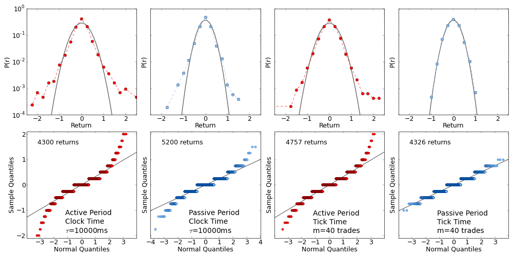
Figure 2: Empirical density and Q-Q plots for clock-time and trade-time returns for both active and passive subsamples. The clock-time interval is $\tau=10000$ milliseconds (10 seconds) and the trade-time interval is $m=40$ (chosen to roughly match the clock-time interval).

The second row of plots in Figure 2 show corresponding quantile-quantile (Q-Q) plots of the distributions in the upper panels. Q-Q plots compare the quantiles of two distributions and are an powerful way to visualize points of departure between them without transforming the data to a logarithmic scale as we did in the upper panels. Hence, the bottom row plots the empirical quantiles of each dataset against the theoretical quantiles of the Gaussian distribution obtained via maximum likelihood (although the quantiles on the x-axis have been standardized). If the theoretical and empirical densities coincide, their quantiles will exhibit a linear relationship. Departures are highlighted via nonlinearities in the Q-Q plot.

As we will see in more detail below, Figure 2 shows that clock-time intra-day returns have heavy tails for both active and passive time periods, which indicates that the probability distribution generating the data has higher probabilities of extreme events than a Gaussian distribution (even during passive, non-event periods). The same is true of active-period trade-time returns. The characteristic heavy tails of the empirical distributions are visible in the Q-Q plots as a convex-concave departure from linearity. Remarkably, the empirical density and corresponding Q-Q plot in the last column of Figure 2 show that passive-period, trade-time returns conform very closely to a Gaussian distribution – they do not have the same propensity for extreme events as the other datasets. This is a key result of our analysis, and we analyze it in more detail in the forthcoming sections. For the remainder of this section, we will depict distributional differences via Q-Q plots.

Figure 3 shows Q-Q plots of clock-time and trade-time returns during active and passive periods for all time scales that we consider. The panels in the first and second rows of the figure compare the empirical quantiles of the clock-time returns with the theoretical quantiles of the best-fit Gaussian distributions for active and passive periods, respectively. The panels in the third and fourth rows are the same for trade-time returns.

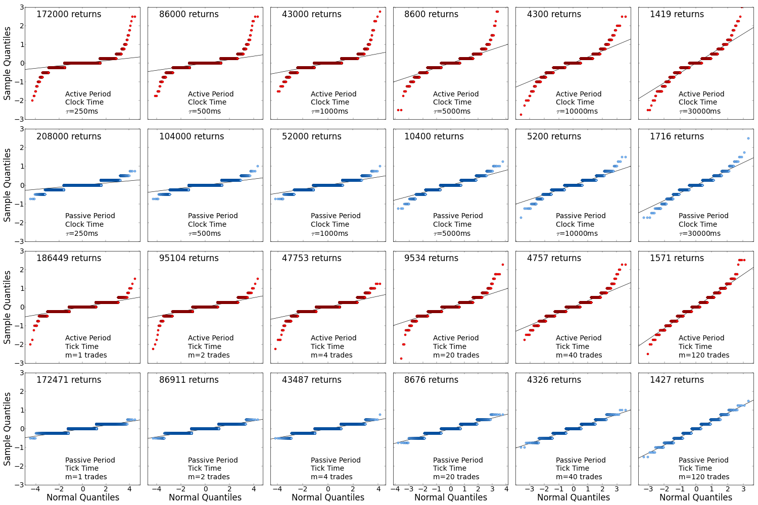
Figure 3: Sample Q-Q plots for returns in both clock time and tick time and in both active and passive subsamples. Each panel corresponds to a clock-time or trade-time interval during either the active or passive subsample of data. The vertical axes depict sample quantiles of the data and the horizontal axes depict theoretical quantiles of best-fit Gaussian distributions.

Not surprisingly, the upper rows of Figure 3 show that clock-time returns distributions are markedly different from a Gaussian density, over a variety of intra-day time scales. In fact, the patterns exhibited in each of the panels are indicative of heavy tails, especially at fine time scales, while as $\tau$ increases the leptokurtosis diminishes. In addition to the diminishing tail weight with increasing $\tau$, comparison of active-period and passive-period clock-time returns shows that active, news-event periods have much heavier tails. This is exactly as we would anticipate, since periods following news announcements should have a higher frequency of large price movements.

The third row of Figure 3 shows that trade-time returns during the active subsample are quite similar to those of clock-time returns during active and passive subsamples: leptokurtosis diminishing with $m$. The final row of the figure, however, highlights the surprising result noted above: during passive, non-event time periods, trade-time returns conform quite closely to a Gaussian distribution. We emphasize that this empirical result has very important asset pricing implications. In fact, Gaussianity of trade-time returns, controlling for known news announcements, will be foundational for the model and results we present in Sections 4 and 5.

Gaussianity of trade-time returns is not immediately apparent when studying intra-day data because trading during news event periods has a large impact on the unconditional distribution of returns. For considerations of space, we have not included Q-Q plots for the full sample of data (without sorting on news events), however the corresponding empirical distributions look quite similar to those we have shown for the active subsample. That is, trading during limited periods of pre-scheduled news announcements has a very large impact on the tail probabilities of the unconditional returns distributions. In contrast, as the bottom panels of Figure 3 indicate, if one only considers returns during non-event times, a Gaussian distribution provides an excellent fit. Knowing that asset returns accumulated in trade time follow a Gaussian distribution during quiescent periods of market activity is a very powerful result.

Figures 4 and 5 depict sample autocorrelation functions (ACFs) of returns and squared returns (respectively) for the clock-time and trade-time intervals considered in the Q-Q plots of Figure 3. It is generally accepted that asset returns exhibit no significant autocorrelation except at very fine time scales, where bid/offer bounce and mean reversion induce negative correlation among adjacent trades. Figure 4 corroborates these stylized facts: at all but the finest time scales and lowest lags, returns show no autocorrelation. For both active and passive periods, autocorrelations of trade-time returns appear to be more muted than those of clock-time returns. In fact, for $\tau=250$ms and $\tau=500$ms, clock-time returns exhibit significant and decaying autocorrelation beyond the first lag, a feature which is not present in the trade-time data, or at least only mildly so for $m=1$ (where there appears to be a very small, significant lag-2 autocorrelation).

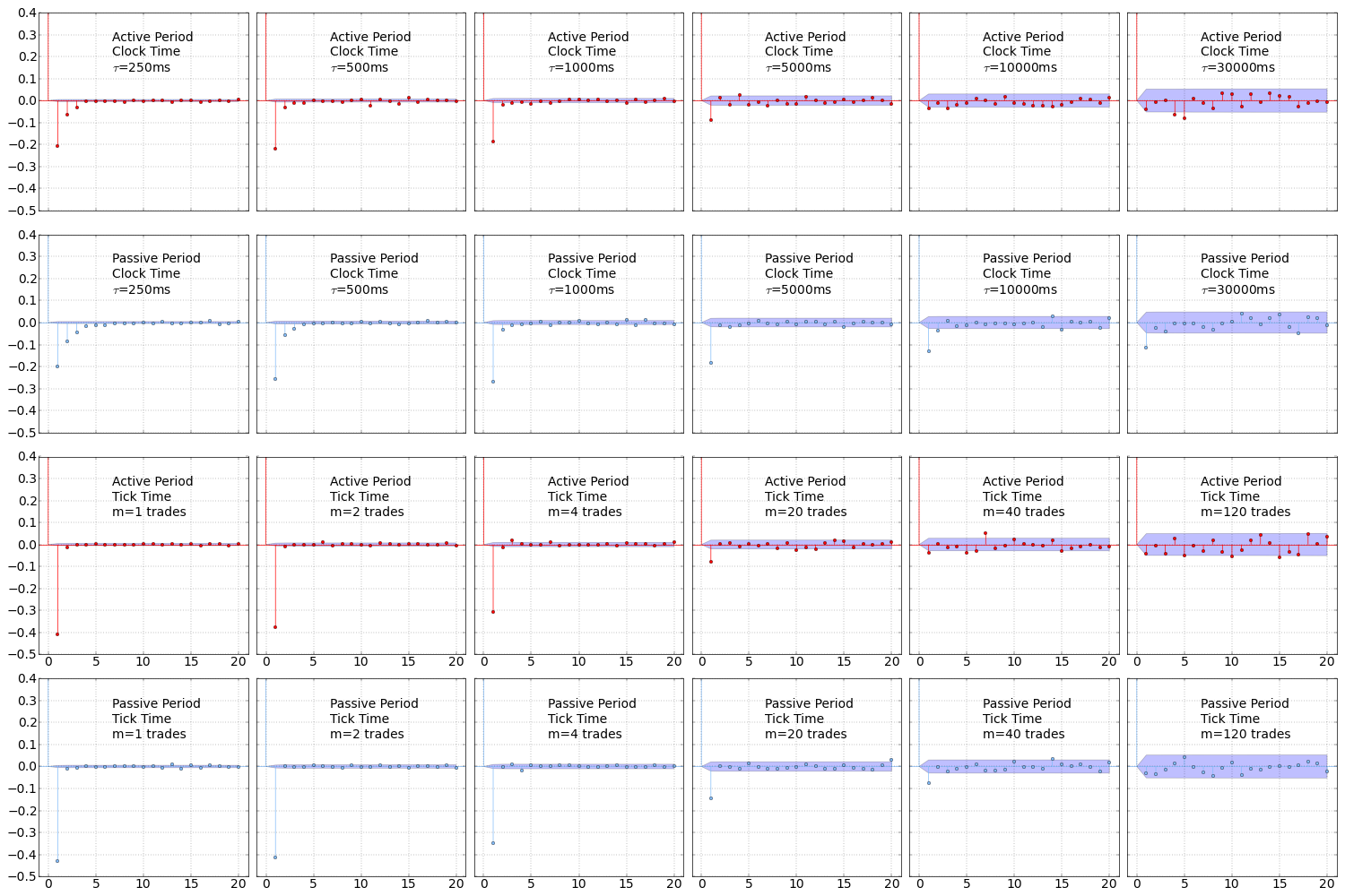
Figure 4: Sample autocorrelation plots for returns in both clock time and trade time and in both active and passive subsamples. Each panel corresponds to a clock-time or trade-time interval during either the active or passive subsample of data.

ACFs of squared returns, shown in Figure 5, are typically used to diagnose the persistence of volatility, which is a well documented property of financial asset returns. In particular, the panels in the second row of Figure 5, which correspond to passive-period, clock-time returns, are exemplary of the persistent nature of volatility. The remaining panels show that active-period returns (both in clock time and in trade time) exhibit volatility peristence, but of a somewhat less consistent nature, and that passive-period, trade-time returns only exhibit a small degree volatility persistence at fine time scales, with the persistence quickly diminishing as $m$ increases. This latter results is a feature of the data will allow us to approximate passive-period, trade-time returns as independent draws from a Gaussian distribution and will facilitate the task of building a Monte Carlo approximation of the clock-time returns distribution in Section 5.

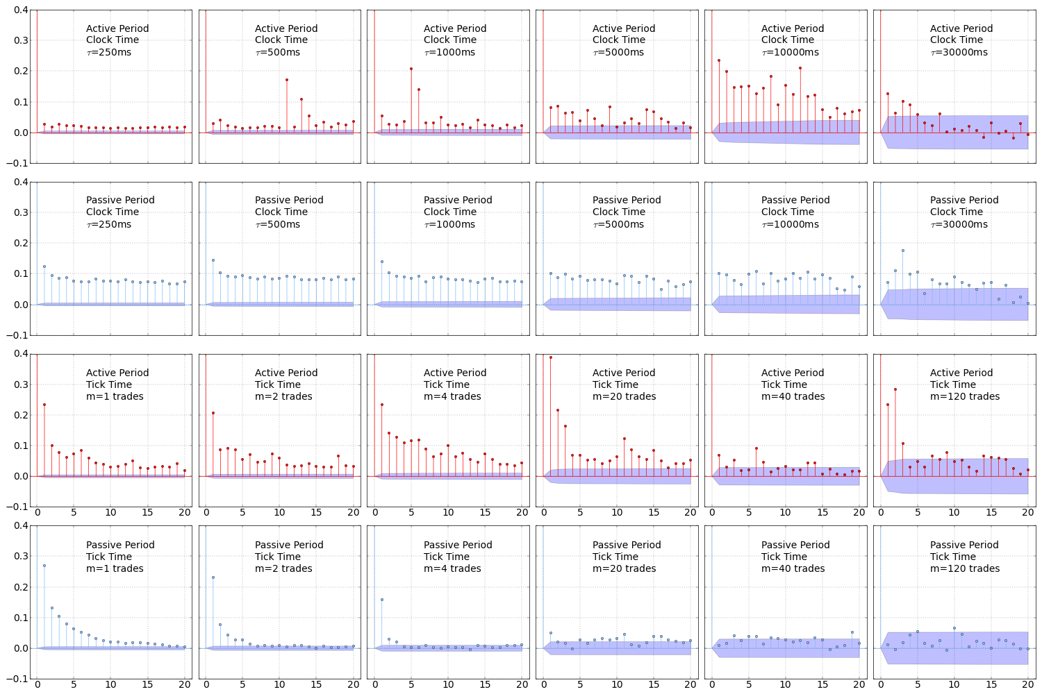
Figure 5: Sample autocorrelation plots for squared returns in both clock time and trade time and in both active and passive subsamples. Each panel corresponds to a clock-time or trade-time interval during either the active or passive subsample of data.

4 Model

In this section we develop a hierarchical model of clock-time returns that mixes a distribution of trade-time returns with a distribution of trade arrivals. For a given trade-time interval $m$, we assume that trade-time returns are independently drawn from a Gaussian distribution,

$$r_{m}(n)\stackrel{{\scriptstyle i.i.d.}}{{\sim}}\mathcal{N}(\mu,\sigma),\forall n.$$ (3)

According to Equation (3), when $m=1$ the price differences between each transaction result in Gaussian returns. However, our notation generalizes to allow price differences across every $m$ transactions to follow a Gaussian distribution, which is direct result of Gaussian aggregation.

Trade arrivals will be distributed according to a counting process to be specified later. For a given clock-time duration $\tau$, we will denote the number of $m$-period executed trades as $N_{m}(\tau)$, with corresponding probability $P(N_{m}(\tau)=k)$, for $k=\{0,1,2,\ldots\}$. If we only observe returns that are aggregated over time interval $\tau$, then we are interested in the distribution of the random variable

$$r_{\tau}(t)=\sum_{i=1}^{N_{m}(\tau)}r_{m}(n).$$ (4)

The probability density function of $r_{\tau}(t)$ is,

$$p(r_{\tau}(t)|\mu,\sigma) =\sum_{k=1}^{\infty}p\left(\sum_{i=1}^{k}r_{m}(n)\bigg{|}N_{m}(\tau)=k,\mu,\sigma\right)P(N_{m}(\tau)=k).$$ (5)

This distribution is characterized as a finite Gaussian mixture model with mixture weights that vary according to the probability distribution of $N_{m}(\tau)$. The model can also be characterized as a two-stage hierarchical model in which a number of trades is drawn from the distribution of $N_{m}(\tau)$ in the first stage and a single $\tau$-period return is drawn from the Gaussian distribution of $r_{\tau}(t)=\sum_{i=1}^{N_{m}(\tau)}r_{m}(n)\sim\mathcal{N}\left(N_{m}(\tau)\mu,\sqrt{N_{m}(\tau)}\sigma\right)$ in the second stage. In the remainder of this section, we consider special cases of Equation (5) under differing assumptions for the distribution of $N_{m}(\tau)$.

4.1 Compound Poisson Process

A starting point for modeling trade arrivals would be to assume they follow a Poisson process:

$$N_{m}(\tau)\sim\rm{Poisson}(\gamma\tau)$$

or

$$P\left(N_{m}(\tau)=k\right)=\frac{(\gamma\tau)^{k}}{k!}\exp\{-\gamma\tau\},$$ (6)

where $\gamma$ is the arrival intensity parameter. In this case Equation (5) becomes

$$p(r_{\tau}(t)|\mu,\sigma) =\sum_{k=1}^{\infty}\frac{1}{\sigma\sqrt{2\pi k}}\exp\left\{-\frac{1}{2}\frac{(\sum_{i=1}^{k}r_{m}(n)-k\mu)^{2}}{k\sigma^{2}}\right\}\times\exp\{-\gamma\tau\}\frac{(\gamma\tau)^{k}}{k!}.$$ (7)

This is a version of the compound Poisson process developed by Press (1967) and Press (1968). Unfortunately, its density function cannot be obtained in closed form. However, the density can be easily approximated by Monte Carlo simulation: first making independent draws from the Gaussian distribution and then accumulating random numbers of those Gaussians according to integer deviates drawn from the Poisson density. Alternatively, in some cases we can approximate Equation (7) with an analytical formula: when $\tau$ is large relative to $\gamma$, the $\mathcal{N}(\gamma\tau,\sqrt{\gamma\tau})$ density serves as good approximation to the $\rm{Poisson}(\gamma\tau)$ density. In this special case, $r_{\tau}(t)$ is also approximately distributed as a Gaussian (compounding two Gaussian densities together in this manner results in another Gaussian density). However, for small values of $\tau$ (when the analytic Gaussian approximation does not hold), the resulting distribution of $r_{\tau}(t)$ exhibits leptokurtosis. Thus, as we will see below, Poisson trade arrivals over short time horizons are able to partially explain extreme events for asset returns although they are inadequate for explaining volatility clustering.

It is important to note that the assumption of Poisson trade arrivals implies that inter-trade durations are distributed as an Exponential random variable, with rate $\gamma$. In Section 5 we will estimate the parameters of this model. We will see that although the Exponential model of trade durations (Poisson model of trade arrival) can partially explain the heavy tails of returns distributions and volatility clustering, it is under-dispersed relative to the actual distribution of trade durations and cannot fully account for those features of the data. Hence, a better model of inter-trade duration is needed to adequately explain observed data.

4.2 Compound Multifractal Process

Chen et al. (2013) develops a model for inter-trade durations that more adequately explains the dynamics of intra-day trade arrivals. The model of that paper, the Markov-switching multifractal duration (MSMD) model, builds on the multifractal volatility model of Calvet and Fisher (2001), Calvet and Fisher (2002) and Calvet (2004). In particular, the authors adapt the multifractal volatility model to explain trade durations (rather than volatility) as aggregates of latent shocks. They demonstrate that the MSMD does quite well at explaining intra-day trade data for a variety of equities traded in 1993.

The core components of the MSMD model are a set of $\bar{k}$ latent state variables, $M_{k,i}$, that obey a two-state Markov-switching process with varying degrees of persistence, $\gamma_{k}$, for $k=1,2,\ldots,\bar{k}$. That is, the distribution of trade durations, $d_{i}$, is governed by the equations,

$$\ d_{i}=\frac{\varepsilon_{i}}{\lambda_{i}}$$ (8a)

$$\varepsilon_{i}\sim Exp(1)$$ (8b)

$$\lambda_{i}=\lambda\prod_{k=1}^{\bar{k}}M_{k,i}$$ (8c)

$$M_{k,i}=\begin{cases}M&\text{with probability}\,\,\gamma_{k}\\ M_{k,i-1}&\text{otherwise}\end{cases}$$ (8d)

$$\gamma_{k}=1-(1-\gamma_{\bar{k}})^{b^{k-\bar{k}}}$$ (8e)

$$M=\begin{cases}m_{0}&\text{with probability}\,\,1/2\\ 2-m_{0}&\text{otherwise}.\end{cases}$$ (8f)

Hence, the MSMD can be succinctly characterized by five parameters: $\bar{k}\in\mathbb{N}$, $\lambda>0$, $\gamma_{\bar{k}}\in(0,1)$, $b\in(1,\infty)$ and $m_{0}\in(0,2]$. The intuition is that conditional on knowing the values of the latent state variables, inter-trade durations are Exponentially distributed with intensity parameter $\lambda_{i}$. However, as time evolves, the latent states, $M_{k,i}$, switch values with varying degrees of persistence, $\gamma_{k}$. This causes the unconditional distribution of trade durations to be a mixture of Exponentials, which is consistent with the over-dispersion property of observed data, described in Section 4.4. The latent states can be interpreted as shocks that have varying impacts over diverse timescales, some having short-horizon and others have long-horizon effects. The value $b$ governs a tight relationship between the persistence parameters, $\gamma_{k}$, and is responsible for the parsimony of the model: even with a large number of latent states, $\bar{k}$, the model is always characterized by a total of five parameters. The choice of $b$ dictates the degree of heterogeneity in values of persistence parameters. For more insight regarding the MSMD model, see Chen et al. (2013) and Calvet and Fisher (2008).

Figure 6 is analogous to Figure 5 in Chen et al. (2013). It shows a simulation of MSMD durations (using the $\bar{k}=7$ parameter values in Table 2) and the associated time paths of the latent states as well as the composite intensity parameter $\lambda_{i}$. The penultimate panel of the figure depicts the stochastic intensity parameter (on a log scale), which is driven by the latent states that switch at differing frequencies. This contrasts with a simple Exponential model of inter-trade durations which fixes a constant intensity parameter. The result is that MSMD durations exhibit far greater heterogeneity than those of the constant-intensity Exponential. Chen et al. (2013) liken stochastic intensity in duration models to stochastic volatility in returns models: “Just as stochastic volatility ‘fattens’ Gaussian conditional returns distributions, so too does MSMD ‘over-disperse’ exponential conditional duration distributions.” (p. 9). In fact, as noted below, we find that stochastic intensity plays the dual role of duration over-dispersion and returns tail fattening.

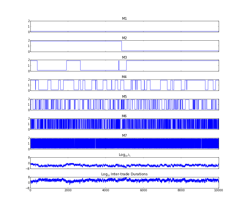
Figure 6: A simulation of MSMD inter-trade durations for $\bar{k}=7$. The upper panels depict the time paths of latent states and MSMD intensity parameter and the bottom panel depicts the durations themselves. The layout of this figure is the same as that presented in Figure 5 of Chen et al. (2013).

Just as the Exponential model of inter-trade durations is tied to the Poisson model of trade arrival, the MSMD model is also tied to a model of trade arrival. As with the Poisson, specifying the probabilities $P(N_{m}(\tau)=k)$, for $k=0,1,2,\ldots$, corresponding to the MSMD model would also result in a distribution for clock-time returns that cannot be obtained in closed form. However, unlike the compound Poisson process, we cannot obtain a closed-form solution for the counting distribution itself which serves as mixture weights in the Gaussian mixture model. Fortunately, we can approximate the counting distribution via Monte Carlo simulation. We show an example of such an approximation in Section 4.4.

The distribution of $r_{\tau}(t)$ retains its hierarchical structure under the MSMD model, with the number of trades per unit of time being drawn from a mixture of Poisson distributions in the first stage. We refer to $r_{\tau}(t)$ as a compound multifractal process when the Gaussian mixture weights correspond to count probabilities associated with MSMD durations. The strength of the compound multifractal process lies in the variability of the underlying counting process: the dispersion of probability over a greater variety of counts, relative to the simple Poisson model, induces greater heterogeneity in the Gaussian mixture, which generates fatter tails for $r_{\tau}(t)$. Intuitively, the random variable $r_{\tau}(t)$ switches between a greater variety of differing sums of Gaussians with higher probability. In addition, the compound multifractal model explicitly generates volatility persistence by producing autocorrelation in the inter-trade duration distribution, via Markov-switching latent states.

4.3 Compound Truncated Multifractal Process

We augment the duration models considered above with a modification of the MSMD model. Specifically, we truncate the MSMD model by mixing it with an Exponential model that is fit so that its expected maximal value is equal to the maximal duration observed in the data. We will provide more detail on the fitting procedure in Section 5. Mathematically,

$$d_{i}=\min\{d_{MSMD},d_{\overline{Exp}}\}$$ (9a)

$$d_{MSMD}\sim MSMD(\bar{k},\lambda,\gamma_{\bar{k}},b,m_{0})$$ (9b)

$$d_{\overline{Exp}}\sim Exp(\nu_{max}),$$ (9c)

where Equation (9b) denotes that $d_{MSMD}$ follows an MSMD process outlined in System (8) and $\nu_{max}$ is chosen so that $\mathbb{E}\,\left[\max\{d_{\overline{Exp}}\}\right]$ equals the maximum duration observed in the data.

The truncated process can be conceptualized as combining two types of traders that are characterized by differing statistical processes. The orders of one type follow the counting process associated with the MSMD model and comprise the majority of trading on exchanges. The orders of the second type follow a simple Poisson event clock and only result in trades when there is a sufficiently long duration between orders of the first type. Intuitively, these types can be thought of as algorithmic traders (following the MSMD counting process), which compete at low latency for order execution, and human traders (following the Exponential), which act independently and exogenously relative to the bulk of trading, and whose orders arrive much less frequently (at longer durations).

As with the MSMD model, the truncated MSMD model is associated with a counting process that can only be obtained via Monte Carlo approximation. Likewise, using the associated truncated MSMD counting process in Equation (5) gives rise to process for $r_{\tau}(t)$ that we refer to as the compound truncated multifractal process. We will show in Sections 4.4 and 5 that this latter model provides a much better description of observed high-frequency returns data.

4.4 Comparison of Duration Models

We now give a brief comparison of the estimated duration models, before describing the estimation results in detail in Section 5. This serves to motivate later discussion and to highlight the strengths and weaknesses of the model components.

Figure 7 shows histograms of 500,000 simulated durations from each of the three models, using the estimated parameters reported in Table 1 (described in Section 5). Each panel depicts the histogram of simulated durations from one model overlaid with the histogram of durations observed in the passive-period E-mini data. We truncate the histograms at 200 ms to focus attention on the regions of greatest probability mass. In addition, to highlight discrepancies in the tails of the distributions, we have shown the vertical axis on a $\log_{10}$ scale.

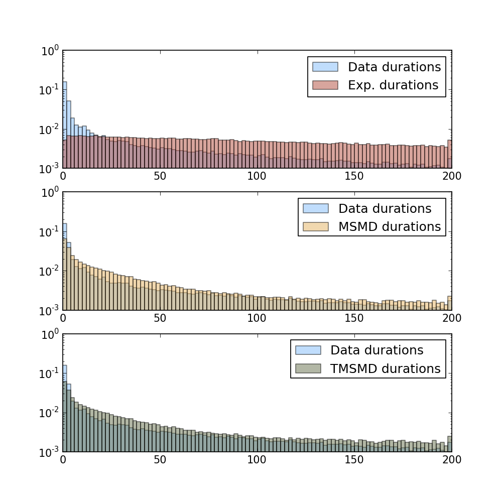
Figure 7: Histograms of simulated durations under the Exponential, MSMD and TMSMD models as well as observed inter-trade durations in the passive-period E-mini returns data.

It is apparent from the figure that the Exponential duration model provides a very poor fit to the distribution of the data relative to the MSMD and truncated MSMD (TMSMD) models. In fact, one important feature exhibited by the latter two models, as in the data, is over-dispersion: that variance of inter-trade durations exceeds their expected value. Under the Exponential model, $\mathbb{E}\,[d_{i}]=\mbox{Var}\,(d_{i})$. However, the asymmetry and long right tail of the distribution of the data yield the empirical result that $\mathbb{E}\,[d_{i}]<\mbox{Var}\,(d_{i})$. This feature is discussed in detail by Chen et al. (2013).

Figure 8 shows Q-Q plots of passive-period observed durations and simulated MSMD and TMSMD durations against simulated Exponential durations. The second panel is a replicate of a the first but with a reduced scale on the vertical axis. Most important to note from the figure is that the empirical distribution of the data has a much heavier tail than the Exponential distribution. This feature is responsible for the over-dispersion discussed above. Further, both the MSMD and TMSMD models produce duration distributions with heavy tails, but the leptokurtosis of the MSMD distribution is excessive relative to that observed in the data. The TMSMD distribution, on the other hand, provides a much closer fit.

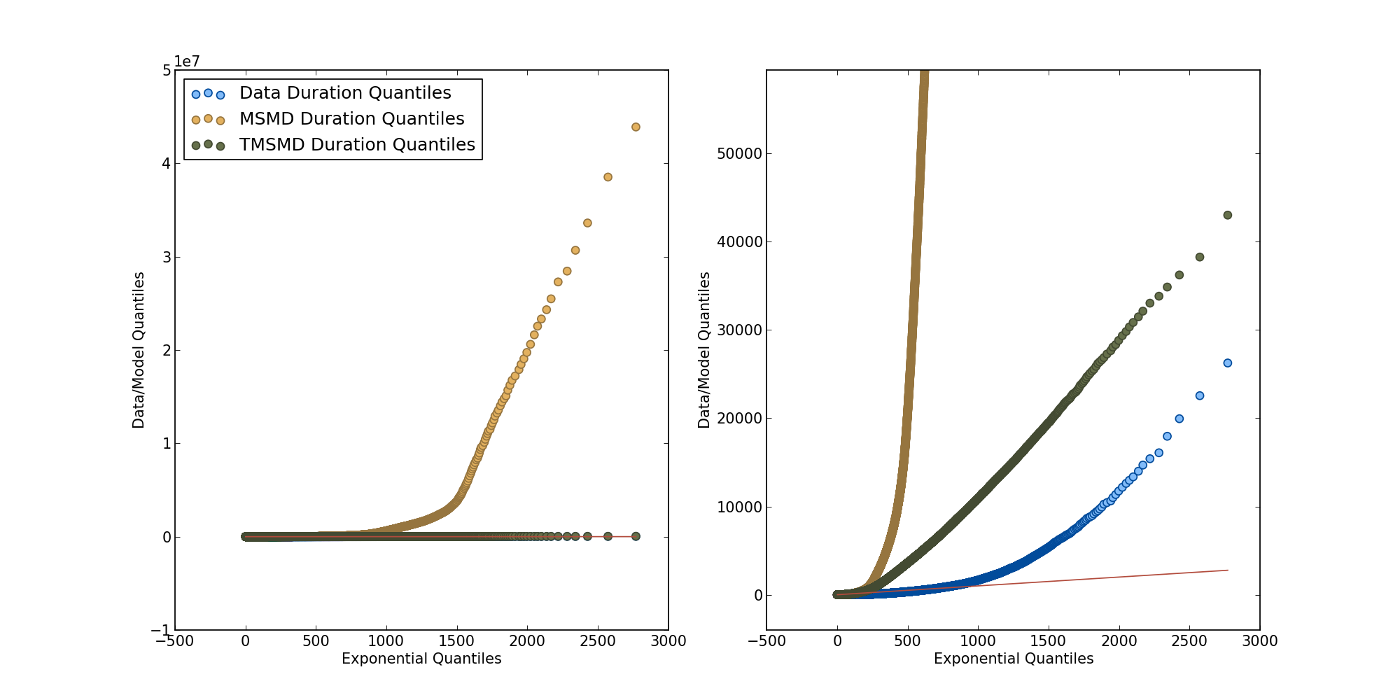
Figure 8: Quantile-Quantile plot. The vertical axis shows quantiles of simulated durations under the MSMD and TMSMD models and observed inter-trade durations in the passive-period E-mini returns data. The horizontal axis shows quantiles of simulated durations under the Exponential model. All model parameters are taken from Table 1.

Another important feature of an inter-trade duration model is the structure of autocorrelations. Figure 9 shows sample autocorrelations computed for 100 lags for each of the model simulations as well as the passive-period E-mini data. As noted by Chen et al. (2013), observed inter-trade durations exhibit slow decay in their autocorrelation structure, suggesting long-memory properties. In contrast, the Exponential model exhibits no autocorrelation since durations are drawn in an i.i.d. fashion from that model. On the other hand, the MSMD and TMSMD models provide a much better fit to the sample autocorrelation function of the data, with the TMSMD strikingly close. Matching both the density function and the autocorrelation function of durations is crucial to generating the dynamics observed in clock-time returns.

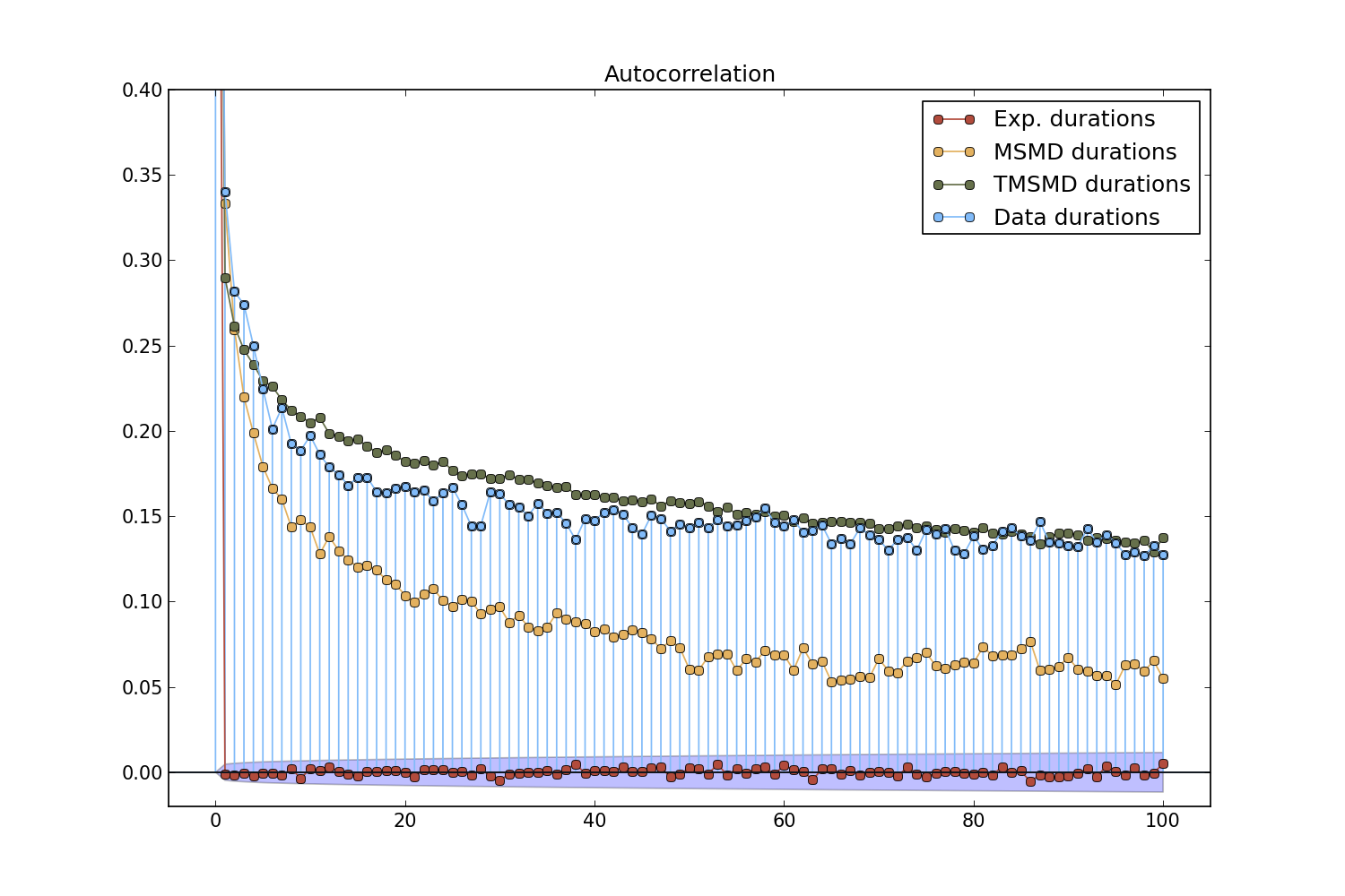
Figure 9: Sample autocorrelation functions of simulated durations under the Exponential, MSMD and TMSMD models as well as observed inter-trade durations in the passive-period E-mini returns data.

Finally, Figure 10 shows the counting densities associated with the duration densities of Figure 7 and a clock-time interval $\tau=10000$ ms. That is, using the data and simulations from each of the models, we obtained respective frequency counts of trade arrivals within consecutive 10000 ms time intervals. To highlight tail discrepancies, we have again shown the vertical axis on a $\log_{10}$ scale. These are approximations of the actual densities used in Equation (5) to obtain the various compound distributions of clock-time returns in Sections 4.1-4.3. Each panel overlays the density associated with a duration model with that of the data. As we mentioned in Section 4.1, the counting process associated with the Exponential duration model is a Poisson process, which is depicted in the first panel of Figure 10. Clearly, the Poisson distribution provides a very poor fit to the data, especially in regions associated with low and high counts. In this particular case the value of $\tau$ is large enough relative to $\lambda$ that the density conforms closely to a Gaussian distribution (recall the the vertical axis is in $\log_{10}$ units). As a result, we expect that the compound Poisson process, which is a mixture of Gaussian and Poisson densities, will not fit the data well and that in this special case they will conform closely to a Gaussian distribution. In contrast, the counting processes associated with MSMD and TMSMD durations provide a much better fit, although their right tails attenuate too quickly relative to the data. Once again, the TMSMD model provides a much better fit to the empirical density of the data.

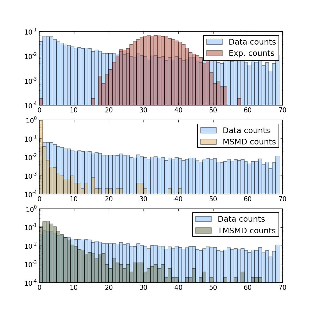
Figure 10: Counting process distributions for $\tau=10000$ ms. Each panel shows the counting distribution associated with one of the simulations (Exponential, MSMD and TMSMD), described in this section, overlaid with the empirical counting density of the passive-period E-mini returns. The simulations were obtained using the parameters estimates reported in Table 1.

5 Estimation and Results

Using the quiescent-market E-mini returns data described in Sections 2 and 3, we estimate the parameters of the component distributions in Equation (5) and simulate from the mixture model. In particular, we first estimate the duration models described in Section 4, which we then compound with an estimated Gaussian distribution for trade-time returns to synthesize a distribution for clock-time returns. Using Monte Carlo approximations for the distribution of clock-time returns, we evaluate the candidate models using several measures of goodness-of-fit and distributional distance.

The choice of trade time scale, $m$, for which we estimate the parameters of the component distributions is not a priori inherent to the model – in theory we could estimate the component distributions for a variety of values for $m$. Instead, we focus exclusively on the finest possible trade time scale, $m=1$, since this most closely mimics the underlying trading process. With the model estimated at such a fine time scale, we can then obtain simulations from the distributions of clock-time returns for any clock-time interval which is of longer duration. This would not be possible if we estimated the trade time components for larger $m$: we would not be able to simulate clock-time returns for clock time scales that are of finer resolution than the chosen $m$. Although we do not report the results here, we have estimated the model for $m>1$ and compared with clock-time simulations of comparable resolutions – the results that we report below are robust to the choice of $m$.

5.1 Poisson/Exponential Estimation

The assumption of Poisson-distributed trade arrivals with mean $\gamma$ corresponds to duration times that are Exponentially distributed with mean $\nu=\frac{1}{\gamma}$. It is trivial to show that the maximum likelihood estimate of the Exponential mean is

$$\hat{\nu}=\frac{1}{\hat{\gamma}}=\frac{1}{n}\sum_{i=1}^{n}d_{i},$$ (10)

where $d_{i}$, $i=1,2,\ldots,n$ are the observed durations for a given trade time scale, $m$.

Columns 1 and 2 of Table 1 report estimates of $\eta$ and $\gamma$ for $m=1$ along with parametric bootstrap estimates of their standard errors. Although estimates of asymptotic standard errors are readily available for these parameters (as well as the parameters of the Gaussian distribution in Section 5.4), we report bootstrap estimates for consistency with the MSMD results below. The reported standard errors are almost identical to their estimated asymptotic counterparts.

Exponential/Poisson		TMSMD	Tick-time Gaussian
$\nu$	$\gamma$	$\nu_{max}$	$\mu$	$\sigma$
300.7	3.326e-03	5866	-7.103e-05	0.1196
(2.405e-03)	(2.642e-08)	NA	(2.928e-04)	(2.072e-04)

Table 1: Estimates of Exponential, Gaussian and TMSMD parameters. For the TMSMD model, $\bar{k}=7$ and the remaining MSMD estimates correspond to those given in Table 2.

It is important to correctly interpret the intensity parameter in Table 1. Since we are now reverting to the assumption that the number of trades arriving in a particular time interval, $\tau$, is distributed as a Poisson, $N_{m}(\tau)$ follows a Poisson process with intensity parameter $\gamma\tau$:

$$N_{m}(\tau)\sim Poisson(\gamma\tau).$$ (11)

Equation (11) says that the number of $m$th trades arriving in an interval, $\tau$, is $Poisson(\gamma\tau)$. In our case, we estimated the Poisson parameter by fixing $m=1$ and a unit time interval as $\tau=1$ millisecond. The resulting estimate $\hat{\gamma}=0.003326$ tells us that we expect roughly 0.003326 trades to arrive each millisecond, or roughly three trades per second. However, given how the Poisson rate parameter scales with time units, this also means that we expect approximately 15 trades in five seconds, 30 trades in ten seconds and so on.

5.2 MSMD Estimation

Following Chen et al. (2013), we evaluate the likelihood of the MSMD model, associated with Equations (8a) – (8f), using the nonlinear filtering method of Hamilton (1989) and maximize the likelihood with a standard hill-climbing algorithm. To estimate all parameters of the MSMD model, we iterate over candidate values of $\bar{k}$ and estimate the remaining four parameters, $\lambda$, $\gamma_{\bar{k}}$, $b$, and $m_{0}$. Table 2 reports these estimates and the value of the log likelihood at the MLEs for $\bar{k}=\{0,1,\ldots,9\}$. We conclude that the likelihood is maximized at $\bar{k}=3$ and declines very slowly for higher values of $\bar{k}$. In our subsequent tests of the model (see Section 5.5), we find that the MSMD model with $\bar{k}=7$ provides a slightly improved fit to the data. This is attributed to the fact that higher values of $\bar{k}$ result in more persistence of the duration process, which subsequently results in greater autocorrelation in the volatility of clock-time returns for $\tau>5000$ ms. Otherwise, the model results and statistical tests are very similar for $\bar{k}\in\{3,4,5,6,7\}$. For purposes of concision, we adopt $\bar{k}=7$ throughout the remainder of this section. The last row of Table 2 reports parametric bootstrap standard errors (using 1000 iterations) for the $\bar{k}=7$ estimates.

MSMD
$\bar{k}$	$\lambda$	$\gamma_{\bar{k}}$	$b$	$m_{0}$	Log likelihood
1	0.1045	0.5922	3.641	0.1259	-1360966
2	0.1039	0.4819	2.286	0.08913	-948840
3	0.09155	0.4656	2.063	0.1502	-940237
4	0.04678	0.5859	4.349	0.1395	-941637
5	0.3338	0.5815	4.269	0.1395	-941641
6	0.1797	0.5870	4.423	0.1388	-941687
7	0.09660	0.5884	4.461	0.1386	-941698
8	0.05190	0.5887	4.471	0.1386	-941700
9	0.3743	0.5883	4.460	0.1386	-941698
Std. Errors ($\bar{k}=7$)	(1.314e-02)	(3.962e-03)	(4.801e-02)	(3.704e-04)

Table 2: Estimates and log likelihood values of MSMD models for $\bar{k}=\{1,\ldots,9\}$.

Figure 11 depicts profiles of the log likelihood in the coordinate directions of the $\bar{k}=7$ parameter estimates reported in Table 2.

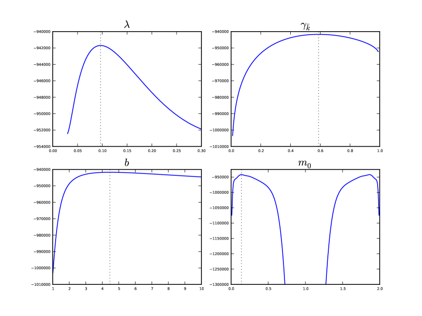
Figure 11: Profiles of the MSMD log-likelihood surface at the achieved maximum (for $\bar{k}=7$) in the coordinate directions of the model parameters.

The profiles show that the log likelihood is smooth and well behaved in the vicinity of the estimates. One interesting feature that we note is the symmetry of the log likelihood with respect to $m_{0}$ – this is a direct result of the fact that the random variable $M$ takes the values $m_{0}$ and $2-m_{0}$ with equal probability. As noted by Chen et al. (2013), the parameters $\gamma_{\bar{k}}$ and $b$ are not identified when $m_{0}=1$, which is manifest as asymptotic behavior in the log-likelihood profile. As a result, two values of $m_{0}$ achieve the maximum and it is irrelevant which we choose. In our application, we have chosen $\hat{m}_{0}\in(0,1)$.

5.3 TMSMD Estimation

Following Section 4.3, the truncated MSMD model is formulated by independently combining the MSMD model with an Exponential distribution that is selected to fit the maximal inter-trade duration observed in the data. Durations under the TMSMD model are simply the minimum of durations generated by the independent components. For this reason, the estimates of the MSMD component are identical to those reported above for the stand-alone MSMD model, again with $\bar{k}=7$.

Our objective in selecting an Exponential distribution for the TMSMD model is to find a random variable, $d_{\overline{Exp}}$, such that

$$d_{\overline{Exp}}\sim Exp(\nu_{max})$$

$$\mathbb{E}\,\left[\max\{d_{\overline{Exp}}\}\right]=d_{max},$$

where $d_{max}=56315$ ms is the longest inter-trade duration observed in our sample of passive-period E-mini data.

Appendix A derives the expectation of $\max\{d_{\overline{Exp}}\}$:

$$\mathbb{E}\,\left[\max\{d_{\overline{Exp}}\}\right] =\nu_{max}\sum_{i=1}^{n}\frac{1}{i}.$$ (12)

We note that the expected value depends on the number of observed durations, which is implicitly a function of the expected duration, $\nu_{max}$, itself. As an approximation, we set $n$ equal to the total time in our data sample (48,600,000 milliseconds) divided by the average duration and rounded to the nearest integer:

$$n =\left[\frac{48,600,000}{\nu_{max}}\right].$$

Thus, to calibrate an appropriate value for $\nu_{max}$ we choose $\hat{\nu}_{max}$ to minimize the function

$$\hat{\nu}_{max} =\underset{\nu}{\text{argmin}}\left\{\left(\nu\sum_{i=1}^{[48600000/\nu]}\frac{1}{i}-56315\right)^{2}\right\}.$$

The numerical solution to this problem is $\hat{\nu}_{max}=5866$ and is reported in Table 1. We do not provide a standard error for this parameter since it is computed via numerical optimization using observed data and is highly sensitive to the total duration time and maximal value of the data. Estimating the standard error via parametric bootstrap would be unreliable due to variation within simulated durations under any candidate model. Truncating the MSMD model of the previous section with this Exponential provides a much better fit to both the tail of the distribution of observed durations as well as their sample autocorrelations, as shown in Section 4.4.

5.4 Trade-time Gaussian Estimation

The key observation of this paper, highlighted in Section 3, is that trade-time returns observed outside of pre-scheduled news periods are well characterized by a Gaussian distribution. Furthermore, the near lack of serial correlation exhibited by the returns and corresponding squared returns indicates that they can be modeled as independent and identically distributed. In this case, the maximum likelihood estimates of the parameters of the distribution are simply the sample average and standard deviation of trade-time returns, measured for a specific value of $m$. The last two columns of Table 1 report these estimates for $m=1$. The corresponding bootstrap standard errors are reported in parentheses below the estimates.

5.5 Simulating Clock-time Returns

With estimates of the component distributions in hand, we obtain Monte Carlo approximations of the clock-time returns distribution using the Gaussian mixture model, expressed in Equation (5). We do this in a hierarchical fashion, first simulating inter-trade durations for $m=1$ from the Exponential, MSMD and TMSMD models, pairing the durations with independent draws of trade-time returns from the estimated Gaussian density, and finally aggregating individual returns within a fixed clock time interval.

Following the procedure outlined above, we aggregate returns for clock-time intervals $\tau=\{250,\allowbreak 500,\allowbreak 1000,\allowbreak 5000,\allowbreak 10000,\allowbreak 30000\}$ milliseconds until we obtain $n=\{208000,\allowbreak 104000,\allowbreak 52000,\allowbreak 10400,\allowbreak 5200,\allowbreak 1716\}$ clock-time returns, respectively, which correspond to the number of observations in the data for those time intervals. The individual simulations under the Exponential, MSMD and TMSMD models use the same trade-time returns; they only differ in the elapsed time between observations. It is important to mention three adjustments that we make in order to simulate clock time returns. First, since E-mini returns are discrete and only observed at increments of 0.25 points, we simulate tick-time returns from the continuous Gaussian distribution described above and then discretize to the nearest 0.25 increment. For example, a simulated tick-time return of 0.13 would be discretized to 0.25, while a simulated tick-time return of 0.12 would be discretized to zero. Second, we perform a similar discretization of simulated durations (under all models) by rounding values to the nearest millisecond. Since zero durations are not allowed in our framework, all simulated durations below one millisecond are rounded upward. Finally, the statistical tests we report below require that the models place probability mass (for the discretized distributions of clock-time returns) on the same support as the empirical density of the data. In some cases, however, aggregated simulated returns under the models are observed outside the set of values observed in the data. In those cases we simply set the returns to zero. While this has the potential to impact the results of the model, in all but one case (noted below) we revise so few of the returns that the adjustment is of little empirical relevance. Table 3 reports the number of values (and their fraction of the total simulation) that were adjusted in this manner, for each model and for each time-scale. The numbers are quite low for fine time scales for all models and increase with $\tau$. The stand-alone MSMD model performs best in this dimension, with virtually no adjustment, while the Exponential model adjusts 16% of returns when $\tau=30000$ ms. For smaller values of $\tau$, however, the Exponential model produces substantially fewer clock-time returns outside the empirical support. Finally, in the worst case ($\tau=30000$ ms) the TMSMD model requires an adjustment of 1.1% of simulated returns, but for all other values of $\tau$ the fraction is well below 1%, often by one or two orders of magnitude.

	$\tau$
	250	500	1000	5000	10000	30000
Exp counts (fraction)	2 (1e-05)	10 (0.0001)	63 (0.00126)	158 (0.0158)	149 (0.0298)	272 (0.16)
MSMD counts (fraction)	0 (0.0)	1 (1e-05)	1 (2e-05)	1.0 (0.0001)	0 (0.0)	0 (0.0)
TMSMD counts (fraction)	35 (0.000175)	40 (0.0004)	47 (0.00094)	24 (0.0024)	15 (0.003)	19 (0.011176)

Table 3: Number (fraction in parentheses) of simulated clock-time returns that were adjusted to fall within the support of discretely observed data values.

Figure 12 shows Q-Q plots of the clock-time returns simulations for each value of $\tau$ that we consider. The panels in the first three rows correspond to the Exponential, MSMD and TMSMD models, respectively. The panels in the final row of the figure are a reproduction of the E-mini passive-period clock-time Q-Q plots shown in Figure 3. It is immediately apparent from the plot that clock-time returns under the MSMD and TMSMD models exhibit heavy tails for all values of $\tau$ while the Exponential model does a very poor job of capturing leptokurtosis, except for the lowest values of $\tau$. This is attributed to the particular nature of the MSMD model: it can be interpreted as a mixture of Exponential distributions, which does a good job of capturing over-dispersion of observed inter-trade durations relative to a simple Exponential. In particular, the persistence of the latent states in the MSMD model generates more variation in inter-trade durations relative to the Exponential distribution, which leads to a more heterogeneous mixture of Gaussian densities in Equation (5), resulting in a greater degree of leptokurtosis.

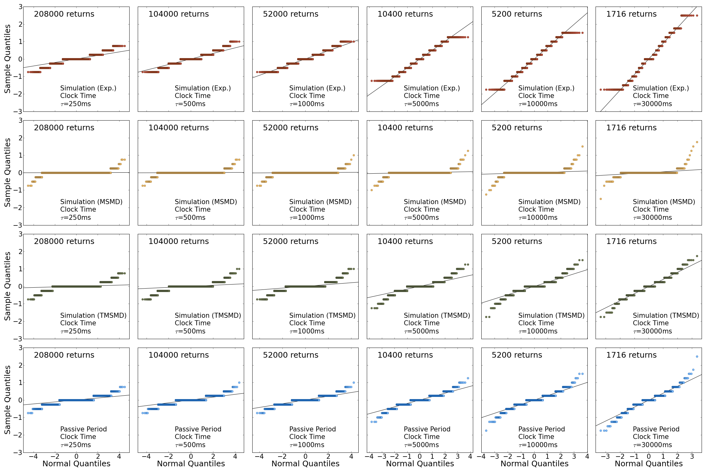
Figure 12: Sample Q-Q plots for simulated clock-time returns. The upper three rows of panels correspond to returns simulated under the Exponential, MSMD and TMSMD models (respectively), for several clock time intervals $\tau$. The bottom row of panels is a reproduction of the E-mini passive-period clock-time Q-Q plots show in Figure 3.

It is also immediately apparent from Figure 12 that the distributions of TMSMD returns are much more similar to the data than those of MSMD returns. In fact, the MSMD returns distributions allocate an excessive portion of probability mass to $r_{\tau}(t)=0$. This is directly attributable to the distribution of MSMD durations, which is depicted in Figures 7 and 8. As seen in those figures, the MSMD distribution has a much heavier right tail than the distribution of the data. This results in a large fraction of trades separated by very long durations, which causes prices to remain constant (zero returns) across clock-time intervals with a frequency that is too high. The TMSMD model rectifies this problem by truncating the long right tail of the MSMD distribution and more closely fitting the tail of the empirical distribution observed in the data. The result is that returns under the TMSMD model conform much more closely to those of the data.

To provide a formal measure of fit, the first three rows of Table 4 report Chi-squared test statistics for returns distributions under each of the three duration models, relative to the empirical distribution of returns. The Chi-squared test is a test of similarity for discrete distributions: under the null hypothesis of identical distributions, a properly weighted sum of the discrepancies in the histograms of each model and the data should be distributed as a $\chi^{2}(k)$, where the degrees of freedom $k$ is one less than the number of histogram bins (unique values that the random variable can assume). Quantiles corresponding to probability 0.95 are reported in the fourth row of Table 4 – Chi-squared test statistics that exceed these values represent a rejection of the null hypothesis at the 5% level.

	$\tau$
	250	500	1000	5000	10000	30000
$\chi^{2}$ Exp	35035.0	63146.0	106900.0	77396.0	48035.0	8680.0
$\chi^{2}$ MSMD	24747.0	20079.0	15229.0	7519.8	5252.7	3039.9
$\chi^{2}$ TMSMD	15462.0	10963.0	6577.7	762.14	85.534	50.68
5% $\chi^{2}_{k}$ critical values	12.592	14.067	14.067	18.307	22.362	24.996
KL Exp	0.032975	0.089006	0.20827	0.50814	0.55751	0.4007
KL MSMD	0.43104	0.62514	0.81613	1.2171	1.2877	1.365
KL TMSMD	0.089029	0.11033	0.11152	0.041454	0.0076904	0.014179

Table 4: Goodness of fit statistics for simulated returns under the Exponential and MSMD duration models. The first three rows report $\chi^{2}$ goodness of fit measures relative to the observed data for each clock time interval $\tau$ that we consider. The latter three rows report Kullback-Leibler divergences, again, relative to the observed data.

The table clearly demonstrates that each of the models fails the Chi-squared goodness-of-fit test at the 5% level for all values of $\tau$. However, this result is not surprising: we know a priori that none of our models is an exact characterization of the true data generating process. Our objective, instead, is to find a model that is a suitable approximation. In this case, with an extremely large dataset, the Chi-squared test is simply informing us that we have a lot of data and that our models are not exactly correct. What is more interesting, however, are the magnitudes of the Chi-squared statistics: the MSMD statistics are uniformly better than those of the Exponential (often by an order of magnitude) and the TMSMD statistics are uniformly better than those of the MSMD (by as much as two orders of magnitude). In fact, while the TMSMD model is rejected for $\tau=10000$ and $\tau=30000$ ms, the Chi-squared statistics are remarkably close to their empirical counterparts when considering the size of the data sample and the simulation.

To provide a another measure of distributional distance, the final three rows of Table 4 report the Kullback-Leibler divergence for the returns distributions under each of the three duration models, relative to the empirical distribution of returns. In contrast to the Chi-squared test, the Kullback-Leibler divergence (see Kullback and Leibler (1951)) is not a statistical test of a formal hypothesis – rather, it is a measure of information loss when using one distribution as an approximation for another. For discrete distributions $F$ and $G$ over values $\{x\}_{i=1}^{n}$, the Kullback-Leibler divergence of $G$ from $F$ is defined as

$$D(F||G) =\sum_{i=1}^{n}\log\left(\frac{F(x_{i})}{G(x_{i})}\right)F(x_{i}),$$

which is the expectation (under distribution $F$) of log probability ratios. In contrast to the magnitudes of the Chi-squared statistics, Table 4 shows that the distribution of returns under the Exponential model is closest to that of the data for $\tau=250$ ms and $\tau=500$ ms and is uniformly closer than the distribution of MSMD returns. However, for larger values of $\tau$, the TMSMD model dominates, often by one or two orders of magnitude. The reason for the failure of the MSMD model under this metric is the high probability mass placed on $r_{\tau}(t)=0$.

Figure 13 shows sample autocorrelation functions for returns simulated under each of the duration models, with each column of panels corresponding to a time scale $\tau=\{250,\allowbreak 500,\allowbreak 1000,\allowbreak 5000,\allowbreak 10000,\allowbreak 30000\}$ milliseconds. As with Figure 12 the first three rows depict autocorrelations under the Exponential, MSMD and TMSMD models, respectively, while the last row is a reproduction of the autocorrelations of E-mini passive-period clock-time returns in Figure 4. Much like the data, the returns ACFs of the models exhibit little autocorrelation, although the MSMD model appears to have a frequency of non-zero autocorrelations that is too high and which exhibit no pattern. While none of the models captures the negative autocorrelation attributed to bid/offer bounce and mean reversion at low lags in finely sampled data (low $\tau$), this dynamic is not explicitly modeled in our framework and is not expected to be present.

Sample autocorrelations of squared returns simulated under each of the models are shown in Figure 14. Persistence among the autocorrelations is present in the MSMD and TMSMD models but not in the Exponential. More importantly, the TMSMD autocorrelations of squared returns conform much more to the data than those of the stand-alone MSMD. This dynamic is a great strength of the framework we promote: the truncated compound multifractal process can jointly explain leptokurtosis and volatility clustering. In particular, Figure 14 shows that autocorrelations of squared returns under the TMSMD model are generally smaller than those of the passive-period E-mini data, but that they exhibit similar decline with increasing time scale, $\tau$.

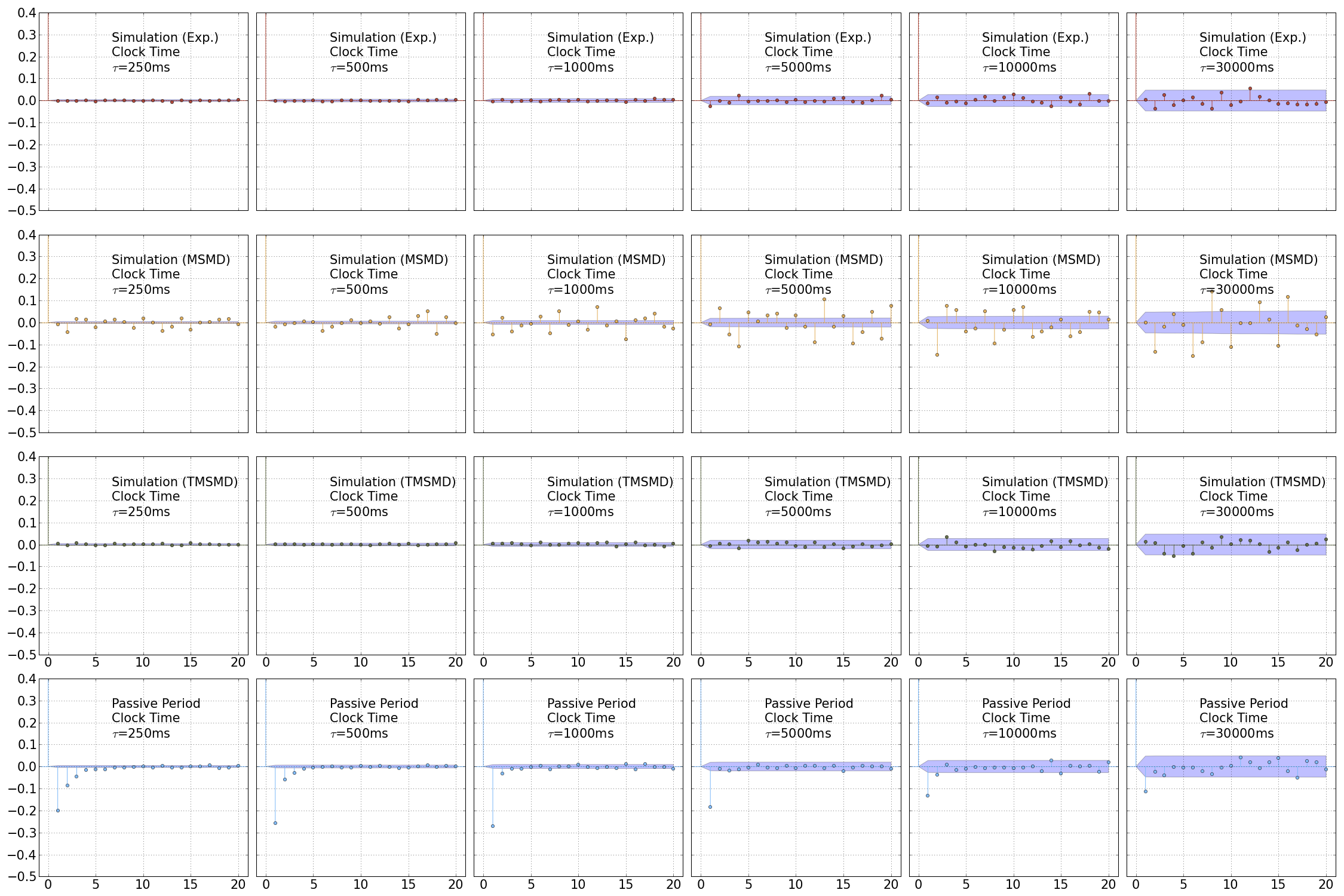
Figure 13: Sample autocorrelation functions for simulated clock-time returns. The upper three rows of panels correspond to returns simulated under the Exponential, MSMD and TMSMD models, for several clock time intervals $\tau$. The bottom row of panels is a reproduction of the autocorrelations of E-mini passive-period clock-time returns in Figure 4.

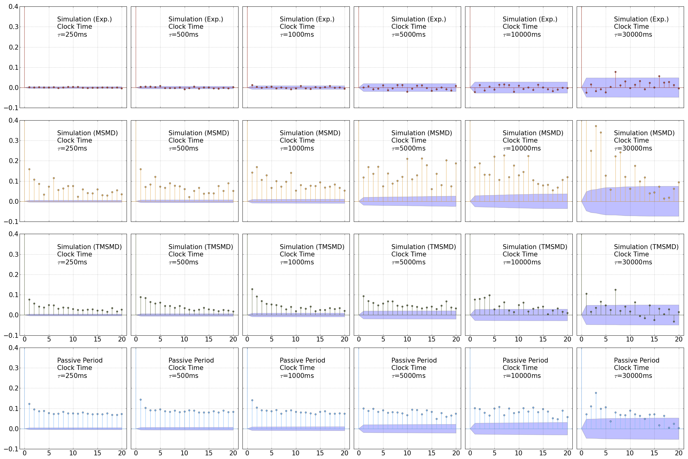
Figure 14: Sample autocorrelation functions for simulated clock-time squared returns. The upper three rows of panels correspond to returns simulated under the Exponential, MSMD and TMSMD models, for several clock time intervals $\tau$. The bottom row of panels is a reproduction of the autocorrelations of E-mini passive-period clock-time squared returns in Figure 5.

As a final measure of model fit, Table 5 reports Ljung-Box statistics for the autocorrelation functions of returns and squared returns, both in the data and under each of the three models. The Ljung-Box statistic is defined as

$$Q =n(n+2)\sum_{i=1}^{l}\frac{\hat{\rho}^{2}_{i}}{n-i},$$

where $\hat{\rho}_{i}$ is the sample autocorrelation for lag $i$, $n$ is the number of observations in the data, and $l$ is the number of lags over which the statistic is computed. Under the null hypothesis that all autocorrelations are jointly zero, $Q\sim\chi^{2}(l)$. For the statistics reported in Table 5 we set $l=20$, but the results were robust to a variety of other choices. This choice of $l$ dictated a common 5% critical value of $\chi^{2}_{0.95}(20)=31.41$.

	$\tau$
	250	500	1000	5000	10000	30000
LB $r_{Exp}$	25.2	28.707	25.64	19.6	18.261	18.848
LB $r_{MSMD}$	860.02	483.01	311.56	95.955	95.207	76.485
LB $r_{TMSMD}$	45.206	53.868	47.937	23.578	20.614	28.109
LB $r_{Data}$	1930.1	351.88	110.36	18.059	28.569	20.303
LB $r_{Exp}^{2}$	32.536	11.004	22.702	16.973	19.24	16.647
LB $r_{MSMD}^{2}$	2397.5	2435.3	1855.0	409.8	452.78	135.69
LB $r_{TMSMD}^{2}$	6559.7	4135.7	1780.7	624.93	345.7	68.076
LB $r_{Data}^{2}$	27412.0	16306.0	6767.5	1249.4	625.47	190.64

Table 5: Ljung-Box statistics for simulated returns under the Exponential, MSMD and TMSMD duration models as well as the observed data for each clock time interval $\tau$ that we consider. The first four rows report Ljung-Box statistics for the ACFs of returns and the last four rows report Ljung-Box statistics for the ACFs of squared returns.

The upper four rows of the Table 5 report Ljung-Box statistics for the ACFs of returns. Interestingly, the data do not pass the test at the 5% level for the lowest three values of $\tau$, due to the large negative autocorrelation attributed to bid/offer bounce and mean reversion. In contrast, the Exponential returns never fail the test and the MSMD returns always fail the test, although their test statistics decline for increasing $\tau$, similar to the data. TMSMD returns fail the test for precisely the same values of $\tau$ as the data, but visual inspection of Figure 13 does not suggest that there is a systematic reason for this. However, for $\tau\geq 5000$ ms, TMSMD returns do not fail the Ljung-Box test and have test statistics that are very similar in magnitude to the data.

The lower four rows of Table 5 report Ljung-Box statistics for the ACFs of squared returns. Both the MSMD and TMSMD models mimic the data and fail the test for all values of $\tau$ while the Exponential model never fails. This is a confirmation of the inability of the compound Poisson process to explain volatility clustering. While the magnitude of the MSMD statistics (for squared returns) are closer to those of the data for $\tau=10000$ ms and $\tau=30000$ ms, the TMSMD statistics follow the data a bit better.

In sum, we find that the truncated compound multifractal model does a good job of capturing both fat tails and volatility persistence in clock time, while leaving the level of returns with almost no autocorrelation. These features are primarily attributed to the underlying MSMD model. The compound Poisson process (corresponding to durations drawn from an Exponential distribution), in contrast, generates clock-time returns that are serially uncorrelated but which do not exhibit volatility persistence nor the fat tails observed in actual data.

6 Application: Price Formation and Equity Market Structure

During trading periods that are not directly associated with news events, the foregoing compound TMSMD/Gaussian model provides a direct connection between the trading rate and the realized volatility of a given security. We now utilize this connection to predict market behavior during periods of stress.

We illustrate this connection with additional historical trading data for the CME E-mini near-month S&P500 futures contract. With the use of the near-month E-mini contract, we are drawing on the same instrument that we used to build our model. We elect, however, to examine a different (and substantially longer) historical range, so that the data is out-of-sample with respect to that used to construct the compound TMSMD/Gaussian model. Specifically, the new data set contains millisecond-stamped trade events for 577 trading sessions between April 27th, 2010 and August 17th 2012. This data spans periods that exhibited substantially higher volatility (such as the days surrounding the Flash Crash in early May 2010, and the market downturn of August 2011) than occurred during our May – August, 2013 in-sample period.

For each of the 577 days in the data set, we collect millisecond-precision time stamps for all E-mini trades occurring between 3:00 p.m. and 4:00 p.m. Eastern Time. This interval corresponds to the last hour of the U.S. equity market trading day. The trading rate is generally high during the last hour of the equity market session and there are very few scheduled market-moving news releases during this daily window. As before, when multiple trades occur during a single millisecond, we aggregate them as a single transaction and use the final, in-force, price of the millisecond as the price of the trade. Finally, we calculate the median inter-trade duration, $\tau_{\rm med}$, among these trades on each day.

For each of the 577 sessions, we also recorded the daily closing prices of the near-month and second-month VX-CBOE Volatility Index Futures, drawing from data published by the CBOE. We then combined the near- and second-month futures closing prices to create a constant weighted-average futures maturity of one month, using the same methodology underlying the iPath S&P 500 VIX Short-Term Futures ETN (ticker symbol VXX). This computation is not an exact replication of the VXX closing price, since it does not account for reverse splits and the daily roll. However, it is a tradeable surrogate for the value of the VIX. The data are shown as gray circles in Figure 15, which presents a clear correlation between volatility futures prices and the E-mini trading rate.

For a specific set of parameters, the compound TMSMD model permits construction of synthetic sequences of clock-time returns and their corresponding annualized volatilities. Using the TMSMD and Gaussian estimates in Tables 1 and 2, we vary the baseline intensity parameter $\lambda\in[0.01,6]$ to map out sequences of returns with the same median durations as those observed in the April 2010 – August, 2012 data and then compute the model-implied annualized volatility corresponding to each median trade duration. These values are depicted in Figure 15 as green circles for the TMSMD model with $\bar{k}=5$, along with a cubic polynomial that is fit to the simulated data. The remaining lines on the figure are similar polynomials fit to simulated data under the TMSMD model with $\bar{k}=\{3,4,6,7\}$. The uppermost line corresponds to $\bar{k}=3$ and the bottommost to $\bar{k}=7$. Interestingly, although the TMSMD model with $\bar{k}=7$ provides the best in-sample fit to the May – August, 2013 data (primarily due to the persistence of durations), $\bar{k}=5$ provides the best out-of-sample fit to the trade rate/volatility relationship. In any case, our subset of models sweeps the extent of the observed data and reproduces the general empirical relationship. The TMSMD model also provides a basis for extrapolation into regimes of high and low volatility that were not observed during the 577 trading-day period.

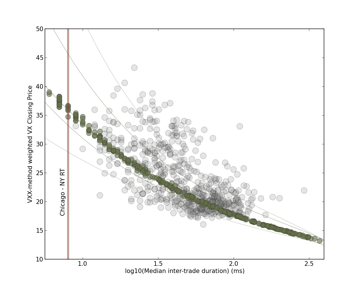
Figure 15: Gray circles: Observed daily closing prices for VX futures (with weightings adjusted to achieve a constant one-month maturity) vs. the daily median inter-trade durations observed for the near-month E-mini S&P 500 futures contract trading from 3:00 p.m. through 4:00 p.m Eastern Time. Green Circles: Annualized volatilities generated from simulations of the TMSMD model ($\bar{k}=5$) driving a Gaussian random walk. The solid lines are cubic polynomial fits to simulated data under the TMSMD model with $\bar{k}=\{3,4,5,6,7\}$. The simulated data is only depicted for $\bar{k}=5$ in order to retain clarity.

Between April 2010 and August 2012, the smallest median inter-trade duration during the last hour of trading occurred on June 6th, 2010, with an observed value of $\tau_{med}=9~{}$ms. The one-month maturity VX-weighted closing price on that day was $V_{\rm VXX}=33.12$. At realized volatilities that are only somewhat larger than those observed in our 577 day sample, our model predicts that the median inter-trade duration at the CME will drop substantially below $\tau_{\rm med}=10~{}$ms. To the extent that the trading activity at the CME is the sole determinant of the E-mini futures price, and assuming that the trading infrastructure itself is able to function smoothly in the presence of increased messaging and computational load, no special change in behavior would be expected for values of $\tau_{\rm med}$ in the $1~{}$ms – $10~{}$ms range.

Indeed, price formation in the U.S. equity market is traditionally assumed to occur in the E-mini contract, as a consequence of the instrument’s composition, its liquidity, and its notional transacted value (Hasbrouck (2003)). The fungibility, however, of the E-mini contract into its 500 component stocks, means that equity trading (either in the component stocks themselves, or in tracking instruments such as SPY (State Street Advisors S&P 500 ETF)) may control a non-negligible fraction of the price discovery process.

The physical separation between the CME order matching engine (located in Aurora, Illinois) and the matching engines for the U.S. equities exchanges (all located in suburban New Jersey) provide an opportunity to quantitatively assess the price discovery process. If one trading venue is responsible for price formation, then price innovations will propagate to outlying exchanges and a clear lead-lag relationship will be established. Laughlin et al. (2014) have shown that price formation can be evaluated by analyzing the lag structure of price-changing trades among highly correlated securities – specifically the E-mini near-month futures contract and the SPY ETF. Recent infrastructure improvements now routinely permit market data and trading orders to flow between physically distant exchanges at nearly the speed of light, which is just above 8 milliseconds round-trip between Aurora, IL and suburban NJ.

To evaluate where price formation actually occurs, we step sequentially through the E-mini trade records within the 577 day data set described above. During periods when both the CME futures exchange and the U.S. equities exchanges are open, we identify in-force prices (the most recent traded price) at the end of each millisecond interval and screen for the occurrence of E-mini trades in which the in-force trade exhibits a change in price over the most recent in-force trade from a previous 1-ms interval.

When a 1-ms interval that ends with a price-increasing in-force E-mini trade has been identified, we search for near-coincident SPY trades in each of the thirty 1-ms intervals prior to and following the E-mini price-changing trade event. If a price-changing SPY trade has occurred, we add the observed change in the SPY traded price ($\delta_{l}$) to an array that maintains a cumulative sum of these price changes from ${\rm lag}=-30~{}{\rm ms}$ to ${\rm lag}=+30~{}{\rm ms}$. The foregoing procedure is also followed for price-decreasing in-force E-mini trades. In the case of these declines, however, we add $-1\times\delta_{l}$ to the array that maintains the cumulative sums. This facilitates the combination of both price increases and price decreases into a single estimator. Our composite response is based on a total of $N$=14,078,656 price-changing E-mini trades observed during the 577-day interval covered by the data and is depicted in Figure 16, where we plot $dP/dt$ for SPY vs. millisecond lag relative to E-mini price-changing trades. It is clear that a larger SPY price response occurs at positive lag, reinforcing the conclusion that price formation occurs primarily, but not completely, at the CME.

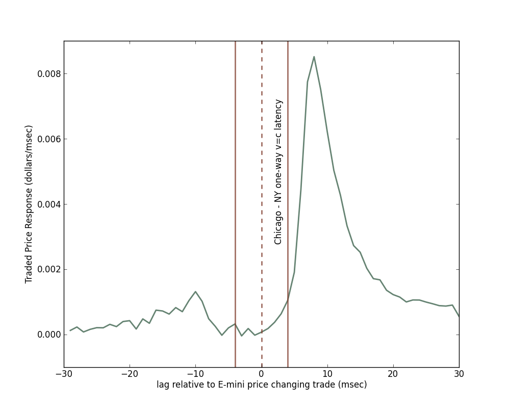
Figure 16: Traded SPY price response to E-mini price-changing trades. The $\pm$4ms light travel times back and forth between Chicago and New York are indicated. The $y$-axis values are normalized to a per price-changing trade basis.

A cumulative positive-lagged response, $\Delta P(t_{f})^{+}$, can be quantified by integrating $dP/dt$ from 0 through lag $t_{f}$,

$$\Delta P(t_{f})^{+}=\int_{0}^{t_{f}}{dP\over{dt}}dt\,,$$

and a cumulative negative-lagged response, $\Delta P(t_{f})^{-}$, can be quantified by integrating $dP/dt$ from 0 through lag $-t_{f}$,

$$\Delta P(t_{f})^{-}=-\int_{-t_{f}}^{0}{dP\over{dt}}dt\,.$$

$\Delta P(t_{f})^{+}$ and $\Delta P(t_{f})^{-}$ are plotted in Figure 17. It is clear that $\Delta P(t_{f})^{+}>\Delta P(t_{f})^{-}$, again indicating that the E-mini is predominantly leading SPY. The ratio ${\mathcal{P}}=\Delta P(t_{f})^{+}/\Delta P(t_{f})^{-}=6.26$ suggests that the E-mini is a factor of ${\mathcal{P}}\sim 6.26$ times more important than SPY in determining price formation. Trading on the equity exchanges thus has a measurable impact, and price discovery is not completely localized at the CME.

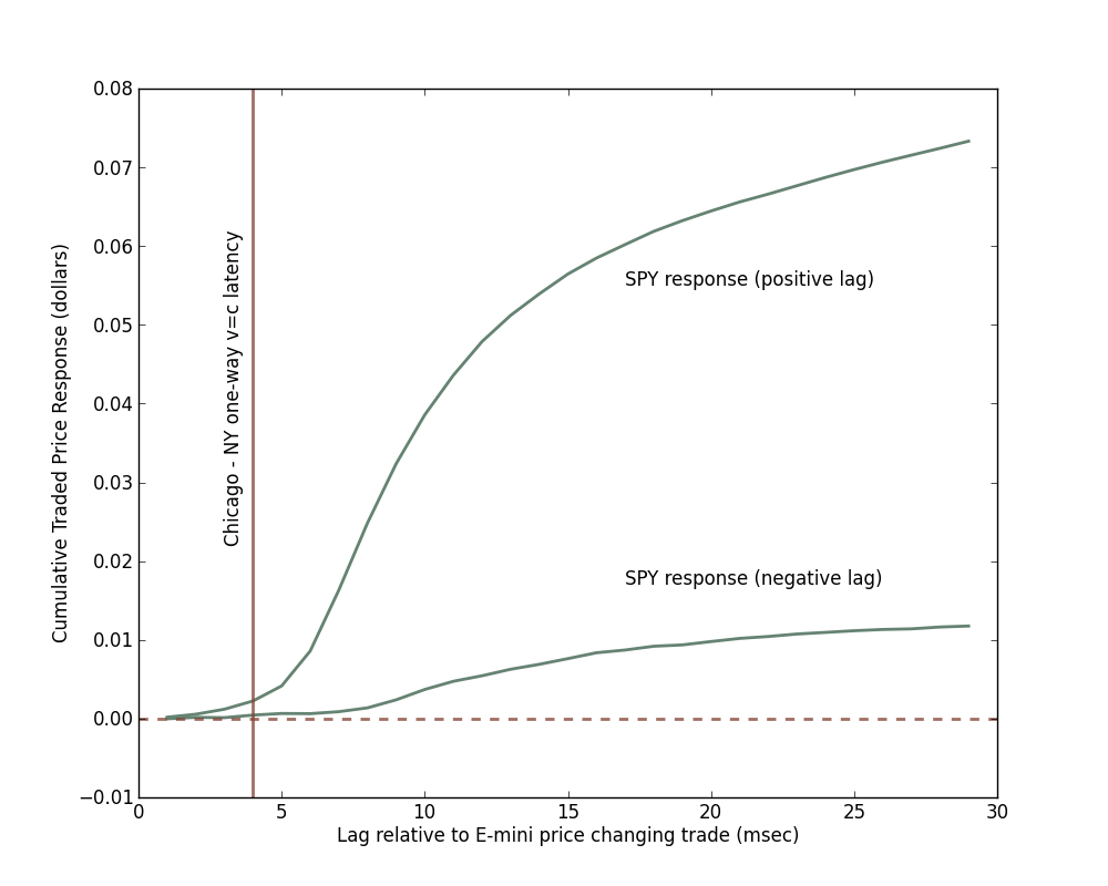
Figure 17: Cumulative Traded SPY price response to E-mini price-changing trades. The integrated SPY response over positive lags is a factor of 6.26$\times$ larger than the integrated SPY response over negative lags.

The sharing of price discovery between exchanges in Chicago and New Jersey and the physical separation of these locations by roughly 1200 km means that the theoretical minimum round-trip time of information flow is about 8 ms. This serves as an effective bound on inter-trade duration, at which point trade rate will saturate. According to the compound TMSMD model, with $\bar{k}=5$, an 8 ms inter-trade duration corresponds to an annualized S&P 500 volatility of approximately 36 percent. With $\bar{k}\leq 4$, the corresponding model-implied volatility is 45 percent or higher.

If underlying market pressure induces the trade rate to push against the current distance-mediated limit, the resulting volatility could lead to a large market move, either up or down. Prior to the SEC imposition of coordinated limit rules among exchanges in April of 2013, such a large market movement could have resulted in an E-mini trading halt at the CME and a subsequent shift in trading interest and price formation to equities exchanges in New Jersey. In such a scenario, the physical separation ($d\leq 56$ km) among exchanges in suburban New Jersey would correspond to a new effective inter-trade duration bound of 0.3 ms or less, which our model suggests is associated with a market volatility substantially greater than 100 percent. Fortunately, as of 8 April, 2013, the SEC has enforced a coordination among circuit breakers that largely precludes such a cascade of events. However, if some other market event resulted in price formation occurring at a single physical location (either Illinois or New Jersey), a period of market stress could lead to an extremely high saturation point for asset trade rate and correspondingly high market volatility.

The upshot is that coordinated limit rules between equities and futures markets may be essential to prevent extreme volatility and potential market failure. While the E-mini and SPY contracts do not represent the entire market, they comprise a substantial fraction of market liquidity and are indicative of what may happen among other assets.

Our model suggests that physical separation of and distributed price formation among exchanges has the benefit of imposing a market-wide volatility ceiling. Our model also suggests that coordinated limit rules among exchanges may be essential for maintaining market stability. In fairness, the model can only be used to extrapolate behavior during quiescent regimes (and not periods that are affected by major news arrivals), when trade-time returns evolve as Gaussian random walks. However, we believe the foregoing results highlight a potential source of market weakness.

7 Conclusion

The empirical and theoretical work of this paper is intimately linked to the work of Mandelbrot (1963), Clark (1973), Brada et al. (1966), Mandelbrot and Taylor (1967) and Ane and Geman (2000), which show that fat-tailed returns distributions are consistent with a Gaussian random walk subordinated by an appropriate stochastic process. Our empirical insight is that after controlling for pre-scheduled, market-wide news announcements, the subordinating process for a highly liquid market aggregate (the E-Mini S&P 500 near-month futures contract) is simply characterized by a model of high-frequency trade arrival. Our theoretical contribution is to develop a parsimonious inter-trade duration model that serves as an appropriate subordinator, and to compose it with a Gaussian random walk to arrive at a hierarchical model of returns in clock time. Specifically, we have found that a modification of the Markov-Switching Multifractal Duration model, developed by Chen et al. (2013), can be tuned to provide a statistically correct description of the trade arrival process. Returns in the tail of the distribution arise as a consequence of the faster random walks generated by periods where the trading rate is high and volatility persistence is generated by correlation among latent Markov-switching shocks. The upshot is that outside of pre-scheduled news-affected periods, the observed non-Gaussianity in the E-mini returns distribution can be fully attributed to the temporal clustering of trades.

We use our model to extrapolate the relationship between inter-trade duration and market volatility and to explore conditions under which market pressure could lead to catastrophically high volatility and potential market failure. We note that this could occur during a period of large market movements and under circumstances that cause price formation to occur at a single physical venue, leading to a reduction in the current distance-mediated effective bound on systemic inter-trade duration. While our model is not tuned to deal explicitly with regimes of market stress, our results may point to a potential for weakness in the current system.

Further work appears warranted. The E-mini attracts a substantial depth of book and routinely exhibits notional trading volumes in excess of 100 billion dollars per day. As such, minor news events, such as those related to a single company, will rarely lead to tangible changes in the index. It is possible, however, that the Gaussian spectrum of tick-time returns is a feature that is largely specific to the heavily traded E-mini. Expanding the work of this paper to a broader set of assets could lead to important innovations to the model. Additionally, it would be useful to adapt the model to explain the evolution of returns under conditions of market stress.

Appendix A Expectation of the Maximum of Exponential Random Variables

Suppose that random variables $\{X_{i}\}_{i=1}^{n}$ are independently and identically distributed as an Exponential with mean parameter $\nu$. Then their common PDF and CDF are

$$f_{X}(x) =\frac{1}{\nu}\exp{\left(-\frac{x}{\nu}\right)}$$

$$F_{Xi}(x) =1-\exp{\left(-\frac{x}{\nu}\right)}.$$

If we let $Y_{n}=\max\{X_{1},X_{2},\ldots,X_{n}\}$, then the CDF of $Y_{n}$ is

$$G_{n}(y) =P(Y_{n}\leq y)$$

$$=P(X_{1}\leq y,X_{2}\leq y,\ldots,X_{n}\leq y)$$

$$=P(X_{1}\leq y)P(X_{2}\leq y)\cdots P(X_{n}\leq y)$$

$$=\prod_{i=1}^{n}F_{X_{i}}(y)$$

$$=F_{X}(y)^{n}$$

$$=\left(1-\exp{\left(-\frac{y}{\nu}\right)}\right)^{n}.$$ (13)

It follows that the PDF of $Y_{n}$ is

$$g_{n}(y) =nF_{X}(y)^{n-1}f_{X}(y)$$

$$=\frac{n}{\nu}\exp{\left(-\frac{y}{\nu}\right)}\left(1-\exp{\left(-\frac{y}{\nu}\right)}\right)^{n-1},$$ (14)

which can be shown to have expectation,

$$\mathbb{E}\,[Y_{n}|\nu] =\int_{0}^{\infty}y\exp{\left(-\frac{y}{\nu}\right)}\left(1-\exp{\left(-\frac{y}{\nu}\right)}\right)^{n-1}dy$$

$$=\nu\sum_{i=1}^{n}\frac{1}{i}.$$ (15)

References

- Aldrich (2013) Aldrich, E. M. (2013), “Trading Volume in General Equilibrium with Complete Markets,” Working Paper.
- Ane and Geman (2000) Ane, T. and Geman, H. (2000), “Order Flow, Transaction Clock, and Normality of Asset Returns,” The Journal of Finance, LV, 2259–2284.
- Bachelier (1900) Bachelier, L. (1900), Théorie de la Spéculation, Paris: Gauthier-Villars.
- Black and Scholes (1973) Black, F. and Scholes, M. (1973), “The Pricing of Options and Corporate Liabilities,” Journal of Political Economy, 81, 637–654.
- Bollerslev (1986) Bollerslev, T. (1986), “Generalized Autoregressive Conditional Heteroskedasticity,” Journal of Econometrics, 31, 307–327.
- Bouchaud (2005) Bouchaud, J.-P. (2005), “The subtle nature of financial random walks.” Chaos, 15, 26104.
- Brada et al. (1966) Brada, J., Ernst, H., and van Tassel, J. (1966), “The Distribution of Stock Price Differences: Gaussian after All?” Operations Research, 14, 334–340.
- Brogaard et al. (2013) Brogaard, J., Hendershott, T., and Riordan, R. (2013), “High Frequency Trading and Price Discovery,” Working Paper.
- Calvet and Fisher (2001) Calvet, L. and Fisher, A. (2001), “Forecasting multifractal volatility,” Journal of Econometrics, 105, 27–58.
- Calvet and Fisher (2002) — (2002), “Multifracticality in Asset Returns: Theory and Evidence,” The Review of Economics and Statistics, 84, 381–406.
- Calvet et al. (1997) Calvet, L., Fisher, A., and Mandelbrot, B. (1997), “Large Deviations and the Distribution of Price Changes,” Cowles Foundation Discussion Paper No. 1165.
- Calvet (2004) Calvet, L. E. (2004), “How to Forecast Long-Run Volatility: Regime Switching and the Estimation of Multifractal Processes,” Journal of Financial Econometrics, 2, 49–83.
- Calvet and Fisher (2008) Calvet, L. E. and Fisher, A. J. (2008), Multifractal Volatility: Theory, Forecasting, and Pricing, Burlington, MA: Academic Press.
- Calvet and Fisher (2012) — (2012), “Extreme Risk and Fractal Regularity in Finance,” SSRN Electronic Journal.
- Chen et al. (2013) Chen, F., Diebold, F. X., and Schorfheide, F. (2013), “A Markov-switching multifractal inter-trade duration model, with application to US equities,” Journal of Econometrics, 177, 320–342.
- Clark (1973) Clark, P. K. (1973), “A Subordinated Stochastic Process Model with Finite Variance for Speculative Prices,” Econometrica, 41, 135–155.
- Easley et al. (2012) Easley, D., de Prado, M. M. L., and O’Hara, M. (2012), “The Volume Clock: Insights into the High Frequency Paradigm,” Journal of Portfolio Management.
- Engle (1982) Engle, R. F. (1982), “Autoregressive Conditional Heteroscedasticity with Estimates of the Variance of United Kingdom Inflation,” Econometrica, 50, 987–1008.
- Fama (1965) Fama, E. F. (1965), “The Behavior of Stock-Market Prices,” The Journal of Business, 38, 34–105.
- Fisher et al. (1997) Fisher, A., Calvet, L., and Mandelbrot, B. (1997), “Multifractality of Deutschemark / US Dollar Exchange Rates ∗,” Cowles Foundation Discussion Paper No. 1165.
- Gallant et al. (1992) Gallant, A. R., Rossi, P. E., and Tauchen, G. (1992), “Stock Prices and Volume,” The Review of Financial Studies, 5, 199–242.
- Ghysels et al. (1995) Ghysels, E., Gouriéroux, C., and Jasiak, J. (1995), “Market Time and Asset Price Movements: Theory and Estimation,” CIRANO Wokring Paper No. 95s-32.
- Hamilton (1989) Hamilton, J. D. (1989), “A New Approach to the Economic Analysis of Nonstationary Time Series and the Business Cycle,” Econometrica, 57, 357–384.
- Hasbrouck (2003) Hasbrouck, J. (2003), “Intraday Price Formation in U.S. Equity Index Markets,” The Journal of Finance, LVIII, 2375–2399.
- Hasbrouck and Saar (2013) Hasbrouck, J. and Saar, G. (2013), “Low-latency trading,” Journal of Financial Markets, 16, 646–679.
- Kullback and Leibler (1951) Kullback, S. and Leibler, R. A. (1951), “On Information and Sufficiency,” The Annals of Mathematical Statistics, 22, 79–86.
- Laughlin et al. (2014) Laughlin, G., Aguirre, A., and Grundfest, J. (2014), “Information Transmission between Financial Markets in Chicago and New York,” The Financial Review, 49, 283–312.
- Mandelbrot (1963) Mandelbrot, B. (1963), “The Variation of Certain Speculative Prices,” The Journal of Business, 36, 394–419.
- Mandelbrot et al. (1997) Mandelbrot, B., Fisher, A., and Calvet, L. (1997), “A Multifractal Model of Asset Returns,” Cowles Foundation Discussion Paper No. 1164.
- Mandelbrot and Taylor (1967) Mandelbrot, B. and Taylor, H. M. (1967), “On the Distribution of Stock Price Differences,” Operations Research, 15, 1057–1062.
- Mandelbrot (1973) Mandelbrot, B. B. (1973), “Comments on: ”A Subordinated Stochastic Process Model with Finite Variance for Speculative Prices,” by Peter K . Clark,” Econometrica, 41, 157–159.
- Press (1967) Press, S. J. (1967), “A Compound Events Model for Security Prices,” The Journal of Business, 40, 317–335.
- Press (1968) — (1968), “A Modified Compound Poisson Process with Normal Compounding,” Journal of the American Statistical Association, 63, 607–613.
- Tauchen and Pitts (1983) Tauchen, G. E. and Pitts, M. (1983), “The Price Variability-Volume Relationship on Speculative Markets,” Econometrica, 51, 485.