Mini-review: Spatial solitons supported by localized gain

Abstract

The creation of stable 1D and 2D localized modes in lossy nonlinear media is a fundamental problem in optics and plasmonics. This article gives a short review of theoretical methods elaborated for this purpose, using localized gain applied at one or several “hot spots” (HSs). The introduction surveys a broad class of models for which this approach was developed. Other sections focus in some detail on basic 1D continuous and discrete systems, where the results can be obtained, partly or fully, in an analytical form (verified by comparison with numerical results), which provides a deeper insight into the nonlinear dynamics of optical beams in dissipative nonlinear media. In particular, considered are the single and double HS in the usual waveguide with the self-focusing (SF) or self-defocusing (SDF) Kerr nonlinearity, which gives rise to rather sophisticated results, in spite of apparent simplicity of the model; solitons attached to a $\mathcal{PT}$-symmetric dipole embedded into the SF or SDF medium; gap solitons pinned to an HS in a Bragg grating (BG); and discrete solitons in a 1D lattice with a “hot site”.

List of acronyms: 1D – one-dimensional; 2D – two-dimensional; b.c. – boundary conditions; BG – Bragg grating; CGLE – complex Ginzburg-Landau equation; CME – coupled-mode equations; HS – hot spot; NLSE – nonlinear Schrödinger equation; $\mathcal{PT}$ – parity-time (symmetry); SDS – spatial dissipative soliton; SF – self-focusing; SDF – self-defocusing; VK – Vakhitov-Kolokolov (stability criterion); WS – warm spot

OCIS numbers: 190.6135; 240.6680; 230.4480; 190.4360

I Introduction and basic models

Spatial dissipative solitons (SDSs) are self-trapped beams of light Rosanov ; MT ; Akhmed or plasmonic waves plas1 -Marini propagating in planar or bulk waveguides. They result from the balance between diffraction and self-focusing (SF) nonlinearity, which is maintained simultaneously with the balance between the material loss and compensating gain. Due to their basic nature, SDSs are modes of profound significance to nonlinear photonics (optics and plasmonics), as concerns the fundamental studies and potential applications alike. In particular, a straightforward possibility is to use each sufficiently narrow SDS beams as signal carriers in all-optical data-processing schemes. This application, as well as other settings in which the solitons occur, stresses the importance of the stabilization of the SDSs modes, and of development of enabling techniques for the generation and steering of such planar and bulk  beams.

In terms of the theoretical description, basic models of the SDS dynamics make use of complex Ginzburg-Landau equations (CGLEs). The prototypical one is the CGLE with the cubic nonlinearity, which includes the conservative paraxial-diffraction and Kerr terms, nonlinear (cubic) loss with coefficient $\epsilon>0$, which represents two-photon absorption in the medium, and the spatially uniform linear gain, with strength $\gamma>0$, aiming to compensate the loss Rosanov ; MT :

$$\frac{\partial u}{\partial z}=\frac{i}{2}\nabla_{\perp}^{2}u-\left(\epsilon-i\beta\right)|u|^{2}u+\gamma u.$$ (1)

Here $u$ is the complex amplitude of the electromagnetic wave in the spatial domain, $z$ is the propagation distance, the paraxial-diffraction operator $\nabla_{\perp}^{2}$ acts on transverse coordinates $\left(x,y\right)$ in the case of the propagation in the bulk, or on the single coordinate, $x$, in the planar waveguide. Accordingly, Eq. (1) is considered as two- or one-dimensional (2D or 1D) equation in those two cases. The equation is normalized so that the diffraction coefficient is $1$, while $\beta$ is the Kerr coefficient, $\beta>0$ and $\beta<0$ corresponding to the SF and self-defocusing (SDF) signs of the nonlinearity, respectively.

A more general version of the CGLE may include an imaginary part of the diffraction coefficient CH ; CGL ; encyclopedia , which is essential, in particular, for the use of the CGLE as a model of the traveling-wave convection Kolodner ; Cross . However, in optical models that coefficient, which would represent diffusivity of photons, is usually absent.

A well-known fact is that the 1D version of Eq. (1) gives rise to an exact solution in the form of an exact chirped SDS, which is often called a Pereira-Stenflo soliton SH ; Lennart :

$$u\left(x,z\right)=Ae^{ikz}\left[\mathrm{sech}\left(\kappa x\right)\right]^{1+i\mu},$$ (2)

$$A^{2}=3\gamma/\left(2\epsilon\right),~{}\kappa^{2}=\gamma/\mu,~{}k=\left(\gamma/2\right)\left(\mu^{-1}-\mu\right),$$ (3)

where the chirp coefficient is

$$\mu=\sqrt{\left(3\beta/2\epsilon\right)^{2}+2}-3\beta/\left(2\epsilon\right).$$ (4)

This exact solution is subject to an obvious instability, due to the action of the uniform linear gain on the zero background far from the soliton’s core. Therefore, an important problem is the design of physically relevant models which may produce stable SDS.

One possibility is to achieve full stabilization of the solitons in systems of linearly coupled CGLEs modeling dual-core waveguides, with the linear gain and loss acting in different cores Dual1 -Dual6 , Marini . This includes, inter alia, a $\mathcal{PT}$-symmetric version of the system that features the exact balance between the gain and loss PT1 ; PT2 . The simplest example of such a stabilization mechanism is offered by the following coupled CGLE system Javid :

$$\frac{\partial u}{\partial z} = \frac{i}{2}\nabla_{\perp}^{2}u-\left(\epsilon-i\beta\right)|u|^{2}u+\gamma u+i\lambda v,$$ (5)

$$\frac{\partial v}{\partial z} = \left(iq-\Gamma\right)v+i\lambda u,$$ (6)

where $\lambda$ is the linear-coupling coefficient, $v\left(x,z\right)$ and $\Gamma>0$ are the electromagnetic-wave amplitude and the linear-loss rate in the stabilizing dissipative core, and $q$ is a possible wavenumber mismatch between the cores. In the case of $q=0$, the zero background is stable in the framework of Eqs. (5) and (6) under condition

$$\gamma<\Gamma<\lambda^{2}/\gamma.$$ (7)

The same ansatz (2) which produced the Pereira-Stenflo soliton for the uncoupled CGLE yields an exact solution of the coupled system (5), (6):

$$\left\{u\left(x,z\right),v\left(x,z\right)\right\}=\left\{A,B\right\}e^{ikz}\left[\mathrm{sech}\left(\kappa x\right)\right]^{1+i\mu},$$ (8)

with chirp $\mu$ given by the same expression (4) as above, and

$$B=i\lambda\left[\Gamma+i\left(k-q\right)\right]^{-1}A.$$ (9)

A stable soliton is obtained if a pair of distinct solutions are found, compatible with the condition of the stability for the zero background [which is Eq. (7) in the case of $q=0$], instead of the single solution in the case of Eq. (3). Then, the soliton with the larger amplitude is stable, coexisting, as an attractor, with the stable zero solution, while the additional soliton with a smaller amplitude plays the role of an unstable separatrix which delineates the boundary between attraction basins of the two coexisting stable solutions Javid .

In the case of $q=0$, the aforementioned condition of the existence of two solutions reduces to

$$\gamma\Gamma\left(1-\mu^{2}\right)>4\mu^{2}\left[\left(\lambda^{2}-\gamma\Gamma\right)+2\Gamma\left(\Gamma-\gamma\right)\right].$$ (10)

In particular, it follows from Eq. (10) and (4) that a related necessary condition, $\mu<1$, implies $\epsilon<3\beta$, i.e., the Kerr coefficient, $\beta$, must feature the SF sign, and the cubic-loss coefficient, $\epsilon$, must be sufficiently small in comparison with $\beta$. If inequality $\mu<1$ holds, and zero background is close to its stability boundaries, i.e., $0<\Gamma-\gamma\ll\gamma$ and $0<\lambda^{2}-\gamma\Gamma\ll\gamma^{2}$, see Eq. (7), parameters of the stable soliton with the larger amplitude are

$$\kappa_{\mathrm{st}}\approx\sqrt{\frac{\gamma}{\mu}}\frac{1-\mu^{2}}{1+\mu^{2}},A_{\mathrm{st}}\approx\sqrt{\frac{3\gamma}{2\epsilon}}\frac{1-\mu^{2}}{1+\mu^{2}},B_{\mathrm{st}}\approx\frac{2\mu}{\left(1-i\mu\right)^{2}}A,$$ (11)

while propagation constant $k$ is given, in the first approximation, by Eq. (3). In the same case, the unstable separatrix soliton has a small amplitude and large width, while its chirp keeps the above value (4):

$$\kappa_{\mathrm{sep}}^{2}\approx\frac{2\left(\Gamma-\gamma\right)}{\gamma\left(1-\mu^{2}\right)}\sqrt{\lambda^{2}-\gamma\Gamma},~{}k_{\mathrm{sep}}\approx\sqrt{\lambda^{2}-\gamma\Gamma},$$ (12)

$$A_{\mathrm{sep}}^{2}\approx\frac{3\mu}{2\epsilon}\kappa_{\mathrm{sep}}^{2},~{}B_{\mathrm{sep}}\approx iA_{\mathrm{sep}},$$ (13)

Getting back to models based on the single CGLE, stable solitons can also be generated by the equation with cubic gain “sandwiched” between linear and quintic loss terms, which corresponds to the following generalization of Eq. (1):

$$\frac{\partial u}{\partial z}=\frac{i}{2}\nabla_{\perp}^{2}u+\left(\epsilon_{3}+i\beta_{3}\right)|u|^{2}u-\left(\epsilon_{5}+i\beta_{5}\right)|u|^{2}u-\Gamma u,$$ (14)

with $\epsilon_{3}>0$, $\epsilon_{5}>0$, $\Gamma>0$, and $\beta_{5}\geq 0$. The linear loss, represented by coefficient $\Gamma$, provides for the stability of the zero solution to Eq. (14). The cubic-quintic (CQ) CGLE was first proposed, in a phenomenological form, by Petviashvili and Sergeev PS . Later, it was demonstrated that the CQ model may be realized in optics as a combination of linear amplification and saturable absorption cqgle2 -cqgle5 . Stable dissipative solitons supported by this model were investigated in detail by means of numerical and analytical methods CQ1 -CQ6 .

The subject of the present mini-review is the development of another method for creating stable localized modes, which makes use of linear gain applied at a “hot spot” (HS), i.e. a localized amplifying region embedded into a bulk lossy waveguide. The experimental technique which allows one to create localized gain by means of strongly inhomogeneous distributions of dopants implanted into the lossy waveguide, which produce the gain if pumped by an external source of light, is well known Kip . Another possibility is even more feasible and versatile: the dopant density may be uniform, while the external pump beam is focused on the location where the HS should be created.

Supporting dissipative solitons by the localized gain was first proposed not in the framework of CGLEs, but for a gap soliton pinned to an HS in a lossy Bragg grating (BG) Mak . In terms of the spatial-domain dynamics, the respective model is based on the system of coupled-mode equations (CMEs) for counterpropagating waves, $u\left(x,z\right)$ and $u\left(x,z\right)$, coupled by the Bragg reflection:

$$iu_{z}+iu_{x}+v+\left(|u|^{2}+2|v|^{2}\right)u=$$

$$-i\gamma u+i\left(\Gamma_{1}+i\Gamma_{2}\right)\delta(x)u,$$ (15)

$$iv_{z}-iv_{x}+u+\left(|v|^{2}+2|u|^{2}\right)v=$$

$$-i\gamma v+i\left(\Gamma_{1}+i\Gamma_{2}\right)\delta(x)v,$$ (16)

where the tilt of the light beam and the reflection coefficients are normalized to be $1$, the nonlinear terms account for the self- and cross-phase modulation induced by the Kerr effect, $\gamma>0$ is the linear-loss parameter, $\Gamma_{1}>0$ represents the local gain applied at the HS [$x=0$, $\delta(x)$ being the Dirac’s delta-function], and the imaginary part of the gain coefficient, $\Gamma_{2}\geq 0$, accounts for a possible attractive potential induced by the HS (it approximates a local increase of the refractive index around the HS).

As was mentioned in Mak too, and for the first time investigated in detail in HSexact , the HS embedded into the usual planar waveguide is described by the following modification of Eq. (1):

$$\frac{\partial u}{\partial z}=\frac{i}{2}\nabla_{\perp}^{2}u-\left(\epsilon-i\beta\right)|u|^{2}u-\gamma u+\left(\Gamma_{1}+i\Gamma_{2}\right)\delta(x)u,$$ (17)

where, as well as in Eqs. (15) and (16), $\Gamma_{1}>0$ is assumed, and the negative sign in front of $\gamma\geq 0$ represents the linear loss in the bulk waveguide. Another HS model, based on the 1D CGLE with the CQ nonlinearity, was introduced in Valery :

$$\frac{\partial u}{\partial z}=\frac{i}{2}\frac{\partial^{2}u}{\partial x^{2}}+i|u|^{2}u-i\beta_{5}|u|^{2}u-\gamma u+\Gamma e^{-x^{2}/w^{2}}|u|^{2}u,$$ (18)

where $\beta_{5}>0$ represents the quintic self-defocusing term, $\gamma>0$ and $\Gamma>0$ are, as above, strengths of the bulk losses and localized cubic gain, and $w$ is the width of the HS (an approximation corresponding to $w\rightarrow 0$, with the HS in the form of the delta-function, may be applied here too). While solitons in uniform media, supported by the cubic gain, are always unstable against the blowup in the absence of the quintic loss Kramer , the analysis reported in Valery demonstrates that, quite counter-intuitively, stable dissipative localized modes in the uniform lossy medium may be supported by the unsaturated localized cubic gain in the model based on Eq. (18).

In addition to the “direct” linear gain assumed in the above-mentioned models, losses in photonic media may be compensated by parametric amplification, which, unlike the direct gain, is sensitive to the phase of the signal param1 ; param2 . This mechanism can be used for the creation of a HS, if the parametric gain is applied in a narrow segment of the waveguide. As proposed in Ye , the respective 1D model is based on the following equation, cf. Eqs. (17) and (18):

$$\frac{\partial u}{\partial z}=\frac{i}{2}\frac{\partial^{2}u}{\partial x^{2}}+i|u|^{2}u-\left(\epsilon-i\beta\right)|u|^{2}u-\left(\gamma-iq\right)u+\Gamma e^{-x^{2}/w^{2}}u^{\ast},$$ (19)

where $u^{\ast}$ is the complex conjugate field, $q$ is a real phase-mismatch parameter, and, as well as in Eq. (18), the HS may be approximated by the delta-function in the limit of $w\rightarrow 0$.

Models combining the localized gain and the uniformly distributed Kerr nonlinearity and linear loss have been recently developed in various directions. In particular, 1D models with two or multiple HSs spotsExact1 -spotsExact2 and periodic amplifying structures KKV ; Yingji , as well as extended patterns Zezyu1 ; Zezyu2 , have been studied, chiefly by means of numerical methods. The numerical analysis has made it also possible to study 2D settings, in which, most notably, stable localized vortices are supported by the gain confined to an annular-shaped area 2D1 -2D6 . The parametric amplification applied at a ring may support stable vortices too, provided that the pump 2D beam itself has an inner vortical structure Ye2 .

Another ramification of the topic is the development of symmetric combinations of “hot” and “cold” spots, which offer a realization of the concept of $\mathcal{PT}$-symmetric systems in optical media, that were proposed and built as settings integrating the balanced spatially separated gain and loss with a spatially symmetric profile of the local refractive index linPT1 -linPT4 . The study of solitons in nonlinear $\mathcal{PT}$-symmetric settings has drawn a great deal of attention nonlinPT1 -nonlinPT5 , PT1 ; PT2 . In particular, it is possible to consider the 1D model in the form of a symmetric pair of hot and cold spots described by two delta-functions embedded into a bulk conservative medium with the cubic nonlinearity Stuttgart . A limit case of this setting, which admits exact analytical solutions for $\mathcal{PT}$-symmetric solitons, corresponds to a $\mathcal{PT}$ dipole, which is represented by the derivative of the delta-function in the following 1D equation Thawatchai :

$$i\frac{\partial u}{\partial z}=-\frac{1}{2}\frac{\partial^{2}u}{\partial x^{2}}-\sigma|u|^{2}u-\varepsilon_{0}u\delta\left(x\right)+i\gamma u\delta^{\prime}\left(x\right).$$ (20)

Here $\sigma=+1$ and $-1$ correspond to the SF and SDF bulk nonlinearity, respectively, $\varepsilon_{0}\geq 0$ is the strength of the attractive potential, which is a natural conservative component of the $\mathcal{PT}$ dipole, and $\gamma$ is the strength of the $\mathcal{PT}$ dipole.

It is also natural to consider discrete photonic settings (lattices), which appear, in the form of discrete CGLEs, as models of arrayed optical discrCGL1 -discrCGL10 or plasmonics plasmon-array2 ; plasmon-array3 waveguides. In this context, lattice counterparts of the HSs amount to a single discr or several discr2 amplified site(s) embedded into a 1D or 2D discr3 lossy array. Being interested in tightly localized discrete states, one can additionally simplify the model by assuming that the nonlinearity is carried only by the active cores, which gives rise to the following version of the discrete CGLE, written here in the general 2D form discr3 :

$$\frac{du_{m,n}}{dz}=\frac{i}{2}\left(u_{m-1,n}+u_{m+1,n}+u_{m,n-1}+u_{m,n+1}-4u_{m,n}\right)$$

$$-\gamma u_{m,n}+\left[\left(\Gamma_{1}+i\Gamma_{2}\right)+\left(iB-E\right)|u_{m,n}|^{2}\right]\delta_{m,0}\delta_{n,0}u_{m,n}\;,$$ (21)

where $m,n=0$, $\pm 1$, $\pm 2$, … are discrete coordinates on the lattice, $\delta_{m,0}$ and $\delta_{n,0}$ are the Kronecker’s symbols, and the coefficient of the linear coupling between adjacent cores is scaled to be $1$. As above, $\gamma>0$ is the linear loss in the bulk lattice, $\Gamma_{1}>0$ and $\Gamma_{2}\geq 0$ represent the linear gain and linear potential applied at the HS site ($m=n=0$), while $B$ and $E$ account for the SF ($B>0$) or SDF ($B<0$) Kerr nonlinearity and nonlinear loss ($E>0$) or gain ($E<0$) acting at the HS (the unsaturated cubic gain may be a meaningful feature in this setting discr3 ).

The $\mathcal{PT}$ symmetry can be introduced too in the framework of the lattice system. In particular, a discrete counterpart of the 1D continuous model (20) with the $\mathcal{PT}$-symmetric dipole was recently elaborated in Raymond :

$$i{\frac{du_{n}}{dz}}=-\left(C_{n,n-1}u_{n-1}+C_{n+1,n}u_{n+1}\right)-g_{n}|u_{n}|^{2}u_{n}+i\kappa_{n}u_{n},$$ (22)

where the $\mathcal{PT}$ dimer (discrete dipole) embedded into the Hamiltonian lattice is represented by $\kappa_{n}=+\kappa$ at $n=0$, $-\kappa$ at $n=1$, and $0$ at $n\neq 0,1$. A counterpart of the delta-functional attractive potential in Eq. (20) corresponds to a local defect in the inter-site couplings: $C_{1,0}=C_{d}$, $C_{n,n-1}=C_{0}\neq C_{d}$ at $n\neq 1$. Lastly, the nonlinearity is assumed to be carried solely by the dimer embedded into the lattice: $g_{n}=g$ at $n=0,1$, and $0$ at $n\neq 0,1$, cf. Eq. (21). Equation (22) admits exact analytical solutions for all $\mathcal{PT}$-symmetric and antisymmetric discrete solitons pinned to the dimer.

In addition to the HS, one can naturally define a “warm spot” (WS), in the 2D CGLE with the CQ nonlinearity, where the coefficient of the linear loss is given a spatial profile with a minimum at the WS ($\mathbf{r}=0$) Skarka . The equation may be taken as the 2D version of Eq. (14) with

$$\Gamma(r)=\Gamma_{0}+\Gamma_{2}r^{2},$$ (23)

where $r$ is the radial coordinate, coefficients $\Gamma_{0}$ and $\Gamma_{2}$ being positive. This seemingly simple model gives rise to a great variety of stable 2D modes pinned to the WS. Depending on values of parameters in Eqs. (14) and (23), these may be simple vortices, rotating elliptic, eccentric, and slanted vortices, spinning crescents, etc. Skarka .

Lastly, the use of the spatial modulation of loss coefficients opens another way for the stabilization of the SDS: as shown in Barcelona , the solitons may be readily made stable if the spatially uniform linear gain is combined with the local strength of the cubic loss, $\epsilon(r)$, growing from the center to periphery at any rate faster than $r^{D}$, where $r$ is the distance from the center and $D$ the spatial dimension. This setting is described by the following modification of Eq. (1):

$$\frac{\partial u}{\partial z}=\frac{i}{2}\nabla_{\perp}^{2}u-\left[\epsilon(r)-i\beta\right]|u|^{2}u+\gamma u,$$ (24)

where, as said above, $\gamma$ and $\epsilon(r)$ are positive, so that $\lim_{r\rightarrow\infty}\left(r^{D}/\epsilon(r)\right)=0$, for $D=1$ or $2$.

This mini-review aims to present a survey of basic results obtained for SDSs pinned to HSs in the class of models outlined above. In view of the limited length of the article, stress is made on the most fundamental results that can be obtained in an analytical or semi-analytical form, in combination with the related numerical findings, thus providing a deep inside into the dynamics of the underlying photonic systems. In fact, the possibility of obtaining many essential results in an analytical form is a certain asset of these models. First, in Section II findings are summarized for the most fundamental 1D model based on Eq. (17), which is followed, in Section III, by the consideration of the $\mathcal{PT}$-symmetric system (20). The BG model (15), (16) is the subject of Section IV, and Section V deals with the 1D version of the discrete model (21). The article is concluded by Section VI.

II Dissipative solitons pinned to hot spots in the ordinary waveguide

The presentation in this section is focused on basic model (17) and its extension for two HSs, chiefly following works HSexact and spotsExact1 , for the settings with a single and double HS, respectively. Both analytical and numerical results are presented, which highlight the most fundamental properties of SDS supported by the tightly localized gain embedded into lossy optical media.

II.1 Analytical considerations

II.1.1 Exact results

Stationary solutions to Eq. (17) are looked for as $u(x,t)=e^{ikz}U(x),$ where complex function $U(x)$ satisfies an ordinary differential equation,

$$\left(\gamma+ik\right)U=\frac{i}{2}\frac{d^{2}U}{dx^{2}}-\left(\epsilon-i\beta\right)|U|^{2}U,$$ (25)

at$~{}x\neq 0,$ supplemented by the boundary condition (b.c.) at $x=0$, which is generated by the integration of Eq. (17) in an infinitesimal vicinity of $x=0$,

$$\lim_{x\rightarrow+0}\frac{d}{dx}U(x)=\left(i\Gamma_{1}-\Gamma_{2}\right)U(x=0),$$ (26)

assuming even stationary solutions, $U(-x)=U(x)$.

As seen from the expression for $A^{2}$ in Eq. (3) [recall that Eqs. (1) and (17) have opposite signs in front of $\gamma$], Eq. (25) with $\gamma>0$ and $\epsilon>0$ cannot be solved by a $\mathrm{sech}$ ansatz similar to that in Eq. (2). As an alternative, $\mathrm{sech}$ can be replaced by $1/\sinh$:

$$U(x)=A\left[\sinh\left(\kappa\left(|x|+\xi\right)\right)\right]^{-\left(1+i\mu\right)},$$ (27)

where $\xi>0$ prevents the singularity. This ansatz yields an exact codimension-one solution to Eq. (25) with b.c. (26), which is valid under a special constraint imposed on coefficients of the system:

$$\Gamma_{1}/\Gamma_{2}-2\Gamma_{2}/\Gamma_{1}=3\beta/\epsilon.$$ (28)

Parameters of this solution are

$$A^{2}=\frac{3\gamma}{2\epsilon},~{}\kappa^{2}=\gamma\frac{\Gamma_{2}}{\Gamma_{1}},~{}\mu=-\frac{\Gamma_{1}}{\Gamma_{2}},~{}k=\frac{\gamma}{2}\left(\frac{\Gamma_{2}}{\Gamma_{1}}-\frac{\Gamma_{1}}{\Gamma_{2}}\right),$$ (29)

$$\xi=\frac{1}{2}\sqrt{\frac{\Gamma_{1}}{\gamma\Gamma_{2}}}\ln\left(\frac{\sqrt{\Gamma_{1}\Gamma_{2}}+\sqrt{\gamma}}{\sqrt{\Gamma_{1}\Gamma_{2}}-\sqrt{\gamma}}\right).$$ (30)

The squared amplitude of the solution is

$$\left|U(x=0)\right|^{2}=\left(3/2\epsilon\right)\left(\Gamma_{1}\Gamma_{2}-\gamma\right).$$ (31)

The main characteristic of the localized beam is its total power,

$$P=\int_{-\infty}^{+\infty}\left|u(x)\right|^{2}dx.$$ (32)

For the solution given by Eqs. (27)-(30),

$$P=\left(3/\epsilon\right)\sqrt{\Gamma_{1}}\left(\sqrt{\Gamma_{1}}-\sqrt{\gamma/\Gamma_{2}}\right).$$ (33)

Obviously, solution (27) exists if it yields $\left|U(x=0\right|^{2}>0$ and $P>0$, i.e.,

$$\Gamma_{1}>\left(\Gamma_{1}\right)_{\mathrm{thr}}\equiv\gamma/\Gamma_{2}.$$ (34)

The meaning of threshold condition (34) is that, to support the stable pinned soliton, the local gain ($\Gamma_{1}$) must be sufficiently large in comparison with the background loss, $\gamma$. It is relevant to mention that, according to Eq. (28), the exact solution given by Eqs. (27), (29), and (30) emerges at threshold (34) in the SDF medium, with $\beta<0$, provided that $\gamma<\sqrt{2}\Gamma_{2}^{2}$. In the opposite case, $\gamma>\sqrt{2}\Gamma_{2}^{2}$, the threshold is realized in the SF medium, with $\beta>0$.

II.1.2 Exact results for $\gamma=0$ (no linear background loss)

The above analytical solution admits a nontrivial limit for $\gamma\rightarrow 0$, which implies that the local gain compensates only the nonlinear loss, accounted for by term $\sim\epsilon$ in Eq. (17). In this limit, the pinned state is weakly localized, instead of the exponentially localized one (27):

$$U_{\gamma=0}(x)=\sqrt{\frac{3}{2\epsilon}}\frac{\sqrt{\Gamma_{1}/\Gamma_{2}}}{\left(\left|x\right|+\Gamma_{2}^{-1}\right)^{1+i\mu}}~{},~{}k=0,$$ (35)

with $\mu$ given by expression (29) (an overall phase shift is dropped here). Note that the existence of solution (35) does not require any threshold condition, unlike Eq. (34). This weakly localized state is a physically meaningful one, as its total power (32) converges, $P(\gamma=0)=3\Gamma_{1}/\epsilon$. Note that this power does not depend on the local-potential strength, $\Gamma_{2}$, unlike the generic expression (33).

II.1.3 Perturbative results for the self-defocusing medium

In the limit case when the loss and gain vanish, $\gamma=\epsilon=\Gamma_{1}=0$, solution (27) goes over into an exact one in the SDF medium (with $\beta<0$) pinned by the attractive potential:

$$U(x)=\frac{\sqrt{2k/|\beta|}}{\sinh\left(\sqrt{2k}\left(|x|+\xi_{0}\right)\right)},$$ (36)

$$\xi_{0}=\frac{1}{2\sqrt{2k}}\ln\left(\frac{\Gamma_{2}+\sqrt{2k}}{\Gamma_{2}-\sqrt{2k}}\right),$$ (37)

$$\left|U(x=0)\right|^{2}=|\beta|^{-1}\left(\Gamma_{2}-2k\right),$$ (38)

which in interval $0<k<(1/2)\Gamma_{2}^{2}$ of the propagation constant. The total power of this solution is

$$P_{0}=\left(2/|\beta|\right)\left(\Gamma_{2}-\sqrt{2k}\right).$$ (39)

In the limit of $k=0$, when amplitude (38) and power (39) attain their maxima, the solution degenerates from the exponentially localized into a weakly localized one [cf. Eq. (35)],

$$U_{k=0}(x)=\frac{1}{\sqrt{|\beta|}\left(|x|+\Gamma_{2}^{-1}\right)},$$ (40)

whose total power converges, $P_{0}(k=0)=2\Gamma_{2}/|\beta|$, as per Eq. (39).

The exact solutions given by Eqs. (36)-(40), which are generic ones in the conservative model [no spacial constraint, such as (28), is required], may be used to construct an approximate solution to the full system of Eqs. (25) and (26), assuming that the gain and loss parameters, $\Gamma_{1},$ $\gamma$, and $\epsilon$, are all small. To this end, one can use the balance equation for the total power:

$$\frac{dP}{dz}=-2\gamma P-2\epsilon\int_{-\infty}^{+\infty}\left|u(x)\right|^{4}dx+2\Gamma_{1}\left|u\left(x=0\right)\right|^{2}=0.$$ (41)

The substitution, in the zero-order approximation, of solution (36), (37) into Eq. (41) yields the gain strength which is required to compensate the linear and nonlinear losses in the solution with propagation constant $k$:

$$\Gamma_{1}=\frac{2\gamma}{\Gamma_{2}+\sqrt{2k}}+\frac{2\epsilon}{3|\beta|}\frac{\left(\Gamma_{2}-\sqrt{2k}\right)\left(\Gamma_{2}+2\sqrt{2k}\right)}{\Gamma_{2}+\sqrt{2k}}.$$ (42)

As follows from Eq. (42), with the decrease of $k$ from the largest possible value, $\left(1/2\right)\Gamma_{2}^{2}$, to $0$, the necessary gain increases from the minimum, which exactly coincides with threshold (34), to the largest value at which the perturbative treatment admits the existence of the stationary pinned mode,

$$\left(\Gamma_{1}\right)_{\max}=2\gamma/\Gamma_{2}+2\epsilon\Gamma_{2}/\left(3|\beta|\right).$$ (43)

The respective total power grows from $0$ to the above-mentioned maximum, $2\Gamma_{2}/|\beta|$.

It is expected that, at $\Gamma_{1}$ exceeding the limit value (43) admitted by the stationary mode, the solution becomes nonstationary, with the pinned mode emitting radiation waves, which makes the effective loss larger and thus balances $\Gamma_{1}-\left(\Gamma_{1}\right)_{\max}$. However, this issue was not studied in detail.

The perturbative result clearly suggests that, in the lossy SDF medium with the local gain, the pinned modes exist not only under the special condition (28), at which they are available in the exact form, but as fully generic solutions too. Furthermore, the increase of the power with the gain strength implies that the modes are, most plausibly, stable ones.

II.1.4 Perturbative results for the self-focusing medium

In the case of $\beta>0$, which corresponds to the SF sign of the cubic nonlinearity, a commonly known exact solution for the pinned mode in the absence of the loss and gain, $\gamma=\epsilon=\Gamma_{1}=0$, is

$$U(x)=\sqrt{2k/|\beta|}\mathrm{sech}\left(\sqrt{2k}\left(|x|+\xi_{0}\right)\right),$$ (44)

$$\xi_{0}=\frac{1}{2\sqrt{2k}}\ln\left(\frac{\sqrt{2k}+\Gamma_{2}}{\sqrt{2k}-\Gamma_{2}}\right),$$ (45)

$$\left|U(x=0)\right|^{2}=|\beta|^{-1}\left(2k-\Gamma_{2}\right),$$ (46)

with the total power

$$P_{0}=\left(2/\beta\right)\left(\sqrt{2k}-\Gamma_{2}\right),$$ (47)

which exists for propagation constants $k>\left(1/2\right)\Gamma_{2}^{2}$, cf. Eqs. (36)-(39). In this case, the power-balance condition (41) yields a result which is essentially different from its counterpart (42):

$$\Gamma_{1}=\frac{2\gamma}{\sqrt{2k}+\Gamma_{2}}+\frac{2\epsilon}{3\beta}\frac{\left(\sqrt{2k}-\Gamma_{2}\right)\left(2\sqrt{2k}+\Gamma_{2}\right)}{\sqrt{2k}+\Gamma_{2}}.$$ (48)

Straightforward consideration of Eq. (48) reveals the difference of the situation from that considered above for the SDF medium: if the strength of the nonlinear loss is relatively small,

$$\epsilon<\epsilon_{\mathrm{cr}}=\left(\beta/2\Gamma_{2}^{2}\right)\gamma,$$ (49)

the growth of power (47) from zero at $\sqrt{2k}=\Gamma_{2}$ with the increase of $k$ is initially (at small values of $P_{0}$) requires not the increase of the gain strength from the threshold value (34) to $\Gamma_{1}>\left(\Gamma_{1}\right)_{\mathrm{thr}}$, but, on the contrary, decrease of $\Gamma_{1}$ to $\Gamma_{1}<\left(\Gamma_{1}\right)_{\mathrm{thr}}$ Mak . Only at $\epsilon>\epsilon_{\mathrm{cr}}$, see Eq. (49), the power grows with $\Gamma_{1}$ starting from $\Gamma_{1}=\left(\Gamma_{1}\right)_{\mathrm{thr}}$.

II.1.5 The stability of the zero solution, and its relation to the existence of pinned solitons

It is possible to check the stability of the zero solution, which is an obvious prerequisite for the soliton’s stability, as said above. To this end, one should use the linearized version of Eq. (17),

$$\frac{\partial u_{\mathrm{lin}}}{\partial z}=\frac{i}{2}\frac{\partial^{2}u_{\mathrm{lin}}}{\partial x^{2}}-\gamma u_{\mathrm{lin}}+\left(\Gamma_{1}+i\Gamma_{2}\right)\delta(x)u_{\mathrm{lin}}.$$ (50)

The critical role is played by localized eigenmodes of Eq. (50),

$$u_{\mathrm{lin}}(x,t)=u_{0}e^{\Lambda z}e^{il\left|x\right|-\lambda\left|x\right|},$$ (51)

where $u_{0}$ is an arbitrary amplitude, localization parameter $\lambda$ must be positive, $l$ is a wavenumber, and $\Lambda$ is a complex instability growth rate. Straightforward analysis yields HSexact

$$\lambda-il=\Gamma_{2}-i\Gamma_{1},~{}\Lambda=(i/2)\left(\Gamma_{2}-i\Gamma_{1}\right)^{2}-\gamma.$$ (52)

It follows from Eq. (52) that the stability condition for the zero solution, $\mathrm{Re}\left(\Lambda\right)<0$, amounts to inequality $\gamma>\Gamma_{1}\Gamma_{2},$ which is exactly opposite to Eq. (34). In fact, Eq. (31) demonstrates that the exact pinned-soliton solution given by Eqs. (27)-(30) emerges, via the the standard forward (alias supercritical) pitchfork bifurcation bif , precisely at the point where the zero solution loses its stability to the local perturbation. The above analysis of Eq. (42) demonstrates that the same happens with the perturbative solution (36), (37) in the SDF model. On the contrary, the analysis of Eq. (48) has revealed above that the same transition happens to the perturbative solution (44), (45) in the SF medium only at $\epsilon>\epsilon_{\mathrm{cr}}$, see Eq. (49), while at $\epsilon>\epsilon_{\mathrm{cr}}$ the pitchfork bifurcation is of the backward (alias subcritical bif ) type, featuring the power which originally grows with the decrease of the gain strength. Accordingly, the pinned modes emerging from the subcritical bifurcation are unstable. However, the contribution of the nonlinear loss ($\epsilon>0$) eventually leads to the turn of the solution branch forward and its stabilization at the turning point. For very small $\epsilon$, the turning point determined by Eq. (48) is located at $\Gamma_{1}\approx 4\sqrt{2\gamma\epsilon/\left(3\beta\right)}$, $P_{0}\approx\sqrt{6\gamma/\left(\beta\epsilon\right)}$.

Lastly, note that the zero solution is never destabilized, and the stable pinned soliton does  not emerge, in the absence of the local attractive potential, i.e., at $\Gamma_{2}\leq 0$.

II.2 Numerical results

II.2.1 Self-trapping and stability of the pinned solitons

The numerical analysis of the model based on Eq. (17) was performed with the delta-function replaced by its Gaussian approximation,

$$\tilde{\delta}(x)=\left(\sqrt{\pi}\sigma\right)^{-1}\exp\left(-x^{2}/\sigma^{2}\right),$$ (53)

with finite width $\sigma$. The shape of a typical analytical solution (27)-(31 for the pinned soliton, and a set of approximations to it provided by the use of approximation (53), are displayed in Fig. 1. All these pinned states are stable, as was checked by simulations of their perturbed evolution in the framework of Eq. (17) with $\delta(x)$ replaced by $\tilde{\delta}(x)$.

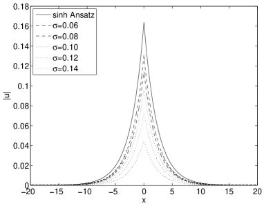
Figure 1: The exact solution for the pinned soliton given by Eqs. (27)-(31), and a set of approximations generated by the regularized delta-function defined as per Eq. (53). All the profiles represent stable solutions. Other parameters are $\beta=0,~{}$ $\gamma=0.25,$ $\Gamma_{1}=0.6155$, and $\Gamma_{2}=\Gamma_{1}/\sqrt{2}$, as per Eq. (28).

The minimum (threshold) value of the local-gain strength, $\Gamma_{1}$, which is necessary for the existence of stable pinned solitons is an important characteristic of the setting, see Eq. (34). Figure 2 displays the dependence of the $\left(\Gamma_{1}\right)_{\mathrm{thr}}$ on the strength of the background loss, characterized by $\sqrt{\gamma}$, for $\beta=0$ and three fixed values of the local-potential’s strength, $\Gamma_{2}=+1,0,-1$ (in fact, the solutions corresponding to $\Gamma_{2}=-1$ are unstable, as they are repelled by the HS). In addition, $\left(\Gamma_{1}\right)_{\mathrm{thr}}$ is also shown as a function of $\sqrt{\gamma}$ under constraint (28), which amounts $\Gamma_{2}=\Gamma_{1}/\sqrt{2}$, in the case of $\beta=0$. The corresponding analytical prediction, as given by Eq. (34), is virtually identical to its numerical counterpart, despite the difference of approximation (53) from the ideal delta-function.

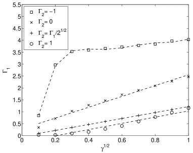
Figure 2: Chains of symbols show the minimum value of the local gain, $\Gamma_{1}$, which is necessary for the creation of stationary pinned solitons in the framework of Eq. (17), as a function of the background loss ($\gamma$), with $\beta=0,$ $\varepsilon=1$, and $\delta(x)$ approximated as per Eq. (53) with $\sigma=0.1$. The strength of the local potential, $\Gamma_{2}$, is fixed as indicated in the box. For $\Gamma_{2}=\pm 1$ and $0,$ the lines are guides for the eye, while the straight line for the case of $\Gamma_{2}=\Gamma_{1}/\sqrt{2}$, which corresponds to Eq. (28) with $\beta=0$, is the analytical prediction given by Eq. (34).

Figure 2 corroborates that, as said above, the analytical solutions represent only a particular case of the family of generic dissipative solitons that can be found in the numerical form. In particular, the solution produces narrow and tall stable pinned solitons at large values of $\Gamma_{1}$. All the pinned solitons, including weakly localized ones predicted by analytical solution (35) for $\gamma=0$, are stable at $\Gamma_{1}>\left(\Gamma_{1}\right)_{\mathrm{thr}}$ and $\Gamma_{2}>0$.

The situation is essentially different for large $\sigma$ in Eq. (53), i.e., when the local gain is supplied in a broad region. In that case, simulations do not demonstrate self-trapping into stationary solitons; instead, a generic outcome is the formation of stable breathers featuring regular intrinsic oscillations, the breather’s width being on the same order of magnitude as $\sigma$, see a typical example in Fig. 3. It seems plausible that, with the increase of $\sigma$, the static pinned soliton is destabilized via the Hopf bifurcation bif which gives rise to the stable breather.

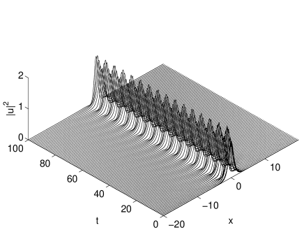
Figure 3: A typical example of a robust breather produced by simulations of Eq. (17) with $\delta(x)$ replaced by approximation $\tilde{\delta}(x)$ as per Eq. (53) with $\sigma=2$, the other parameters being $\beta=\epsilon=\Gamma_{2}=1$, $\Gamma_{1}=4$, and $\gamma=0.1$.

II.3 The model with the double hot spot

The extension of Eq. (17) for two mutually symmetric HSs separated by distance $2L$ was introduced in spotsExact1 :

$$\frac{\partial u}{\partial z}=\frac{i}{2}\frac{\partial^{2}u}{\partial x^{2}}-\gamma u-\left(\epsilon-i\beta\right)|u|^{2}u$$

$$+\left(\Gamma_{1}+i\Gamma_{2}\right)\left[\delta\left(x+L\right)+\delta\left(x-L\right)\right]u.$$ (54)

Numerical analysis has demonstrated that stationary symmetric solutions of this equation (they are not available in an analytical form) are stable, see a typical example in Fig. 4, while all antisymmetric states are unstable, spontaneously transforming into their symmetric counterparts.

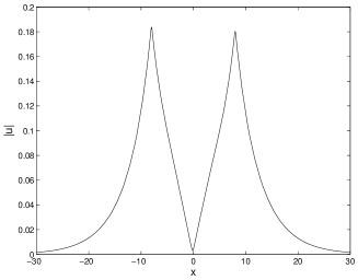
Figure 4: A stable symmetric mode generated by Eq. (54) with the delta-functions approximated as per Eq. (53) with $\sigma=0.1$. Other parameters are $\beta=0,\epsilon=1,\gamma=0.057,\Gamma_{1}=0.334$, $\Gamma_{2}=0.236$, and $L=8$.

As shown above in Fig. 3, Eq. (17) with the single HS described by expression (53), where $\sigma$ is large enough, supports breathers, instead of stationary pinned modes. Simulations of Eq. (54) demonstrate that a pair of such broad HSs support unsynchronized breathers pinned by each HS, if the distance between them is large enough, hence the breathers virtually do not interact. A completely different effect is displayed in Fig. 5, for two broad HSs which are set closer to each other: the interaction between the breathers pinned to each HS transforms them into a stationary stable symmetric mode. It is relevant to stress that the transformation of the breather pinned by the isolated HS into a stationary pinned state does not occur for the same parameters. This outcome is a generic result of the interaction between the breathers, provided that the distance between them is not too large.

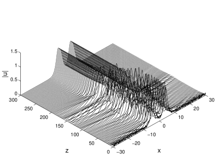
Figure 5: Spontaneous transformation of a pair of breathers pinned to two hot spots, described by Eq. (54), into a stationary symmetric mode. Parameters are $\beta=0$, $\epsilon=1$, $\gamma=1$, $\Gamma_{1}=4$, $\Gamma_{2}=1$, and $L=4$.

II.4 Related models

In addition to the HSs embedded into the medium with the uniform nonlinearity, more specific models, in which the nonlinearity is also concentrated at the HSs, were introduced in spotsExact1 and spotsExact2 . In particular, the respective system with the double HS is described by the following equation:

$$\frac{\partial u}{\partial z}=\frac{i}{2}\frac{\partial^{2}u}{\partial x^{2}}-\gamma u$$

$$+\left[\left(\Gamma_{1}+i\Gamma_{2}\right)-\left(E-iB\right)\left|u\right|^{2}\right]\left[\delta\left(x+L\right)+\delta\left(x-L\right)\right]u,$$ (55)

where $B$ and $E$ are coefficients of the localized Kerr nonlinearity and cubic loss, respectively. These settings may be realized if the nonlinear properties of the waveguides are dominated by narrow doped segments.

Although model (55) seems somewhat artificial, its advantage is a possibility to find both symmetric and antisymmetric pinned modes in an exact analytical form. Those include both fundamental modes, with exactly two local power peaks, tacked to the HSs, and higher-order states, which feature additional peaks between the HSs. An essential finding pertains to the stability of such states, for which the sign of the cubic nonlinearity plays a crucial role: in the SF case [$B>0$ in Eq. (55)], only the fundamental symmetric and antisymmetric modes, with two local peaks tacked to the HSs, may be stable. In this case, all the higher-order multi-peak modes, being unstable, evolve into the fundamental ones. In the case of the SDF cubic nonlinearity [$B<0$ in Eq. (55)], the HS pair gives rise to multistability, with up to eight coexisting stable multi-peak patterns, both symmetric and antisymmetric ones. The system without the Kerr term ($B=0$), the nonlinearity in Eq. (55) being represented solely by the local cubic loss ($\sim E$) is similar to one with the self-focusing or defocusing nonlinearity, if the linear potential of the HS is, respectively, attractive or repulsive, i.e., $\Gamma_{2}>0$ or $\Gamma_{2}<0$ (note that a set of two local repulsive potentials may stably trap solitons in an effective cavity between them Mak ). An additional noteworthy feature of the former setting is the coexistence of the stable fundamental modes with robust breathers.

III Solitons pinned to the $\mathcal{PT}$-symmetric dipole

III.1 Analytical results

The nonlinear Schrödinger equation (NLSE) in the form of Eq. (20) is a unique example of a $\mathcal{PT}$-symmetric system in which a full family of solitons can be found in an exact analytical form Thawatchai . Indeed, looking for stationary solutions with real propagation constant $k$ as $u\left(x,z\right)=e^{ikz}U(x)$, where the $\mathcal{PT}$ symmetry is provided by condition $U^{\ast}(x)=U(-x)$, one can readily find, for the SF and SDF signs of the nonlinearity, respectively,

$$U(x) = \sqrt{2k}\frac{\cos\theta+i~{}\mathrm{sgn}(x)\sin\theta}{\cosh\left(\sqrt{2k}\left(|x|+\xi\right)\right)},\mathrm{~{}for}~{}~{}\sigma=+1,$$ (56)

$$U(x) = \sqrt{2k}\frac{\cos\theta+i~{}\mathrm{sgn}(x)\sin\theta}{\sinh\left(\sqrt{2k}\left(|x|+\xi\right)\right)},~{}\mathrm{for}~{}~{}\sigma=-1,$$ (57)

with real constants $\theta$ and $\xi$, cf. Eq. (27). The form of this solution implies that $\mathrm{Im}\left(U(x=0)\right)=0,$ while jumps ($\Delta$) of the imaginary part and first derivative of the real part at $x=0$ are determined by the b.c. produced the integration of the $\delta$- and $\delta^{\prime}$- functions in an infinitesimal vicinity of $x=0$, cf. Eq. (26):

$$\Delta\left\{\mathrm{Im}\left(U\right)\right\}|_{x=0} = 2\gamma\mathrm{Re}\left(U\right)|_{x=0},$$ (58)

$$\Delta\left\{\left(\frac{d}{dx}\mathrm{Re}\left(U\right)\right)\right\}|_{x=0} = -2\varepsilon_{0}~{}\mathrm{Re}\left(U\right)|_{x=0}.$$ (59)

The substitution of expressions (56) and (57) into these b.c. yields

$$\theta=\arctan\left(\gamma\right),$$ (60)

which does not depend on $k$ and is the same for $\sigma=\pm 1$, and

$$\xi=\frac{1}{2\sqrt{2k}}\ln\left(\sigma\frac{\sqrt{2k}+\varepsilon_{0}}{\sqrt{2k}-\varepsilon_{0}}\right),$$ (61)

which does not depend on the $\mathcal{PT}$ coefficient, $\gamma$.

The total power (32) of the localized mode is

$$P_{\sigma}=2\sigma\left(\sqrt{2k}-\varepsilon_{0}\right).$$ (62)

As seen from Eq. (61), the solutions exist at

$$\left\{\begin{array}[]{cc}\sqrt{2k}>\varepsilon_{0}&\mathrm{for}~{}~{}\sigma=+1,\\ \sqrt{2k}<\varepsilon_{0}&\mathrm{for~{}~{}}\sigma=-1.\end{array}\right.~{}~{}$$ (63)

As concerns stability of the solutions, it is relevant to mention that expression (62) with $\sigma=+1$ and $-1$ satisfy, respectively, the Vakhitov-Kolokolov (VK) VK ; Berge and “anti-VK” anti criteria, i.e.,

$$dP_{+1}/dk>0,~{}dP_{-1}/dk<0,$$ (64)

which are necessary conditions for the stability of localized modes supported, severally, by the SF and SDF nonlinearities, hence both solutions have a chance to be stable.

III.2 Numerical findings

As above [see Eq. (53)], the numerical analysis of the model needs to replace the exact $\delta$-function by its finite-width regularization, $\tilde{\delta}(x)$. In the present context, the use of the Gaussian approximation is not convenient, as, replacing the exact solutions in the form of Eqs. (56) and (57) by their regularized counterparts, it is necessary, inter alia, to replace $\mathrm{sgn}(x)\equiv-1+2\int_{-\infty}^{x}\delta(x^{\prime})dx^{\prime}$ by a continuous function realized as $-1+2\int_{-\infty}^{x}\tilde{\delta}(x^{\prime})dx^{\prime}$, which would be a non-elementary function. Therefore, the regularization was used in the form of the Lorentzian,

$$\delta(x)\rightarrow\frac{a}{\pi}\frac{1}{x^{2}+a^{2}},~{}\delta^{\prime}(x)\rightarrow-\frac{2a}{\pi}\frac{x}{\left(x^{2}+a^{2}\right)^{2}},~{}$$

$$\mathrm{sgn}(x)\rightarrow\frac{2}{\pi}\arctan\left(\frac{x}{a}\right),$$ (65)

with $0<a\ll k^{-1/2}$ Thawatchai .

The first result for the SF nonlinearity, with $\sigma=+1$ (in this case, $\varepsilon_{0}=+1$ is also fixed by scaling) is that, for given $a$ in Eq. (65), there is a critical value, $\gamma_{\mathrm{cr}}$, of the $\mathcal{PT}$ coefficient, such that at $\gamma<\gamma_{\mathrm{cr}}$ the numerical solution features a shape very close to that of the analytical solution (56), while at $\gamma>\gamma_{\mathrm{cr}}$ the single-peak shape of the solution transforms into a double-peak one, as shown in Fig. 6(a). In particular, $\gamma_{\mathrm{cr}}\left(a=0.02\right)\approx 0.24$.

$\begin{array}[]{c}\includegraphics[width=180.67499pt]{Fig6a.pdf}\\ (\mathrm{a})\\ \includegraphics[width=180.67499pt]{Fig6b.pdf}\\ (\mathrm{b})\end{array}$

Figure 6: (Color online) Comparison between the analytical solutions (solid and dotted blue curves show their real and imaginary parts, respectively), given by Eqs. (56), (60), and (61) with $\sigma=+1$ and $\varepsilon_{0}=1$, and their numerically found counterparts, obtained by means of regularization (65) with $a=0.02$ (magenta curves). The $\mathcal{PT}$ parameter is $\gamma=0.20$ in (a) and $0.32$ in (b). In both panels, the solutions are produced for propagation constant $k=3$.

The difference between the single- and double-peak modes is that the former ones are completely stable, as was verified by simulations of Eq. (20) with regularization (65), while all the double-peak solutions are unstable. This correlation between the shape and (in)stability of the pinned modes is not surprising: the single- and double-peak structures imply that the pinned mode is feeling, respectively, effective attraction to or repulsion from the local defect. Accordingly, in the latter case the pinned soliton is unstable against spontaneous escape, transforming itself into an ordinary freely moving NLSE soliton, as shown in Fig. 7.

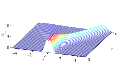
Figure 7: (Color online) The unstable evolution (spontaneous escape) of the double-peak soliton whose stationary form is shown in Fig. 6(b).

Figure 8 summarizes the findings in the plane of $\left(a,\gamma\right)$ for a fixed propagation constant, $k=3.0$. The region of the unstable double-peak solitons is a relatively narrow boundary layer between broad areas in which the stable single-peak solitons exist, as predicted by the analytical solution, or no solitons exist at all, at large values of $\gamma$. Note also that the stability area strongly expands to larger values of $\gamma$ as the regularized profile (65) becomes smoother, with the increase of $a$. On the other hand, the stability region does not vanish even for very small $a$.

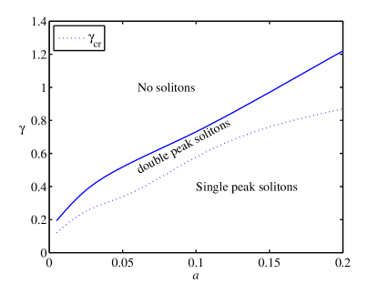
Figure 8: (Color online) Regions of the existence of stable single-peak and unstable double-peak $\mathcal{PT}$-symmetric solitons, separated by $\gamma=\gamma_{\mathrm{cr}}(a)$, in the plane of the regularization scale, $a$, and the gain-loss parameter, $\gamma,$ for fixed $k=3.0$, in the system described by Eqs. (20) and (65) with $\sigma=+1$ (the SF nonlinearity) and $\varepsilon_{0}=1$.

For the same model but with the SDF nonlinearity, $\sigma=-1$, the results are simpler: all the numerically found pinned solitons are close to the analytical solution (57), featuring a single-peak form, and are completely stable.

A generalization of model (20), including a nonlinear part of the trapping potential, was studied in Thawatchai too:

$$i\frac{\partial u}{\partial z}=-\frac{1}{2}\frac{\partial^{2}u}{\partial x^{2}}-\sigma|u|^{2}u-\left(\varepsilon_{0}+\varepsilon_{2}|u|^{2}\right)u\delta\left(x\right)+i\gamma u\delta^{\prime}\left(x\right).$$ (66)

Equation (66) also admits an analytical solution for pinned solitons, which is rather cumbersome. It takes a simpler form in the case when the trapping potential at $x=0$ is purely nonlinear, with $\varepsilon_{0}=0$, $\varepsilon_{2}>0$, Eq. (61) being replaced by

$$\xi=\frac{1}{2\sqrt{2k}}\ln\left[\frac{2\varepsilon_{2}\sqrt{2k}}{1+\gamma^{2}}+\sqrt{1+\frac{8\varepsilon_{2}^{2}k}{\left(1+\gamma^{2}\right)^{2}}}\right]$$ (67)

[it is the same for both signs of the bulk nonlinearity, $\sigma=+1$ and $-1$, while the solution at $x\neq 0$ keeps the form of Eqs. (56) or (57), respectively], with total power

$$P_{\sigma}(k)=2\left[\frac{1+\gamma^{2}}{2\varepsilon_{2}}+\sigma\sqrt{2k}-\sigma\sqrt{2k+\frac{\left(1+\gamma^{2}\right)^{2}}{4\varepsilon_{2}^{2}}}\right].$$ (68)

Note that expressions (67) and (68) depend on the $\mathcal{PT}$ strength $\gamma$, unlike their counterparts (61) (62). Furthermore, solution (67) exists for all values of $k>0$, unlike the one given by Eq. (61), whose existence region is limited by condition (63). The numerical analysis demonstrates that these solutions have a narrow stability area (at small $\gamma$) for the SF bulk medium, $\sigma=+1$, and are completely unstable for $\sigma=-1$.

IV Gap solitons supported by a hot spot in the Bragg grating

As mentioned above, the first example of SDSs supported by an HS in lossy media was predicted in the framework of the CMEs (15) and (16) for the BG in a nonlinear waveguide Mak . It is relevant to outline this original result in the present review. Unlike the basic models considered above, the CME system does not admit exact solutions for pinned solitons, because Eqs. (15) and (16) do not have analytical solutions in the bulk in the presence of the loss terms, $\gamma>0$, therefore analytical consideration (verified by numerical solutions) is only possible in the framework of the perturbation theory, which treats $\gamma$ and $\Gamma_{1}$ as small parameters, while the strength of the local potential, $\Gamma_{2}$, does not need to be small. This example of the application of the perturbation theory is important, as it provided a paradigm for the analysis of other models, where exact solutions are not available either Valery ; Ye .

IV.1 The zero-order approximation

A stationary solution to Eqs. (15) and (16) with $\gamma=\Gamma_{1}=0$ and $\Gamma_{2}>0$ is sought for in the form which is common for quiescent BG solitons Christo -Sterke :

$$u\left(x,z\right)=U(x)\exp\left(-iz\cos\theta\right),$$

$$v(x,z)=-V^{\ast}(x)\exp\left(-iz\,\cos\theta\right),$$ (69)

where $\ast$ stands for the complex conjugate, $\theta$ is a parameter of the soliton family, and function $U(x)$ satisfies equation

$$\left[i\frac{d}{dx}U+\cos\theta+\Gamma_{2}\delta(x)\right]U+3|U|^{2}U-U^{\ast}=0.$$ (70)

The integration of Eq. (70) around $x=0$ yields the respective b.c., $U(x=+0)=U(x=-0)\exp(i\Gamma_{2})$, cf. Eq. (26) . As shown in Mak-earlier , an exact soliton-like solution to Eq. (70), supplemented by the b.c., can be found, following the pattern of the exact solution for the ordinary gap solitons Aceves -Sterke :

$$U(x)=\frac{1}{\sqrt{3}}\frac{\sin\theta}{\cosh\left[\left(|x|+\xi\right)\sin\theta-\frac{i}{2}\theta\right]}\,,$$ (71)

where offset $\xi$, cf. Eqs. (27), (56), (57), is determined by the relation

$$\tanh\left(\xi\sin\theta\right)=\frac{\tan\left(\Gamma_{2}/2\right)}{\tan\left(\theta/2\right)}\,.$$ (72)

Accordingly, the soliton’s squared amplitude (peak power) is

$$\left|U(x=0)\right|^{2}=\left(2/3\right)\left(\cos\Gamma_{2}-\cos\theta\right)\,.$$ (73)

From Eq. (72) it follows that the solution exists not in the whole interval $0<\theta<\pi$, where the ordinary gap solitons are found, but in a region determined by constraint $\tanh\left(\xi\sin\theta\right)<1$, i.e.,

$$\Gamma_{2}<\theta<\pi.$$ (74)

In turn, Eq. (74) implies that the solutions exist only for $0\leq\Gamma_{2}<\pi$ ($\Gamma_{2}<0$ corresponds to the repulsive HS, hence the soliton pinned to it will be unstable).

IV.2 The first-order approximation

In the case of $\gamma=\Gamma_{1}=0$, Eqs. (15) and (16) conserve the total power,

$$P=\int_{-\infty}^{+\infty}\left[\left|u(x)\right|^{2}+\left|v(x)\right|\right]^{2}dx\,.$$ (75)

In the presence of the loss and gain, the exact evolution equation for the total power is

$$\frac{dP}{dz}=-2\gamma P+2\Gamma_{1}\left[\left|u(x)\right|^{2}+\left|v(x)\right|^{2}\right]|_{x=0}\,.$$ (76)

If $\gamma$ and $\Gamma_{1}$ are treated as small perturbations, the balance condition for the power, $dP/dz=0$, should select a particular solution, from the family of exact solutions (71) of the conservative model, which remains, to the first approximation, a stationary pinned soliton, cf. Eq. (41).

The balance condition following from Eq. (76) demands $\gamma P=\Gamma_{1}\left[\left|U(x=0)\right|^{2}+\left|V(x=0)\right|^{2}\right]\,.$ Substituting, in the first approximation, the unperturbed solution (71) and (72) into this condition, it can be cast in the form of

$$\frac{\theta-\Gamma_{2}}{\cos\Gamma_{2}-\cos\theta}=\frac{\Gamma_{1}}{\gamma}\,.$$ (77)

The pinned soliton selected by Eq. (77) appears, with the increase of the relative gain strength $\Gamma_{1}/\gamma$, as a result of a bifurcation. The inspection of Fig. 9, which displays $(\theta-\Gamma_{2})$ vs. $\Gamma_{1}/\gamma$, as per Eq. (77), shows that the situation is qualitatively different for $\Gamma_{2}<\pi/2$ and $\Gamma_{2}>\pi/2$.

In the former case, a tangent (saddle-node) bifurcation bif occurs at a minimum value $\left(\Gamma_{1}/\gamma\right)_{\min}$ of the relative gain, with two solutions existing at $\Gamma_{1}/\gamma>$ $\left(\Gamma_{1}/\gamma\right)_{\min}$. Analysis of Eq. (77) demonstrates that, with the variation of $\Gamma_{2}$, the value $\left(\Gamma_{1}/\gamma\right)_{\min}$ attains an absolute minimum, $\Gamma_{1}/\gamma=1$, at $\Gamma_{2}=\pi/2$. With the increase of $\Gamma_{1}/\gamma$, the lower unstable solution branch, that starts at the bifurcation point [see Fig. 9(a)] hits the limit point $\theta=\Gamma_{2}$ at $\Gamma_{1}/\gamma=1/\sin\Gamma_{2}$, where it degenerates into the zero solution, according to Eq. (73). The upper branch generated, as a stable one, by the bifurcation in Fig. 9(a) continues until it attains the maximum possible value, $\theta=\pi$, which happens at

$$\frac{\Gamma_{1}}{\gamma}=\left(\frac{\Gamma_{1}}{\gamma}\right)_{\max}\equiv\frac{\pi-\Gamma_{2}}{1+\cos\Gamma_{2}}\,.$$ (78)

In the course of its evolution, this branch may acquire an instability unrelated to the bifurcation, see below.

In the case $\Gamma_{2}>\pi/2$, the situation is different, as the saddle-node bifurcation is imaginable in this case, occurring in the unphysical region $\theta<\Gamma_{2}$, see Fig. 9(b). The only physical branch of the solutions appears as a stable one at point $\Gamma_{1}/\gamma=1/\sin\Gamma_{2}$, where it crosses the zero solution, making it the unstable. However, as well as the above-mentioned branch, the present one may be subject to an instability of another type. This branch ceases to be a physical one at point (78). At the boundary between the two generic cases considered above, i.e., at $\Gamma_{2}=\pi/2$, the bifurcation occurs exactly at $\theta=\pi/2$, see Fig. 9(c).

The situation is different too in the case $\Gamma_{2}=0$ [see Fig. 1(d)], when the HS has no local-potential component, and Eq. (77) takes the form of

$$\frac{\theta}{2\sin^{2}\left(\theta/2\right)}=\frac{\Gamma_{1}}{\gamma}\,.$$ (79)

In this case, the solution branches do not cross axis $\theta=0$ in Fig. 9(d). The lower branch, which asymptotically approaches the $\theta=0$ axis, is unstable, while the upper one might be stable within the framework of the present analysis. However, numerical results demonstrate that, in the case of $\Gamma_{2}=0$, the soliton is always unstable against displacement from $x=0$.

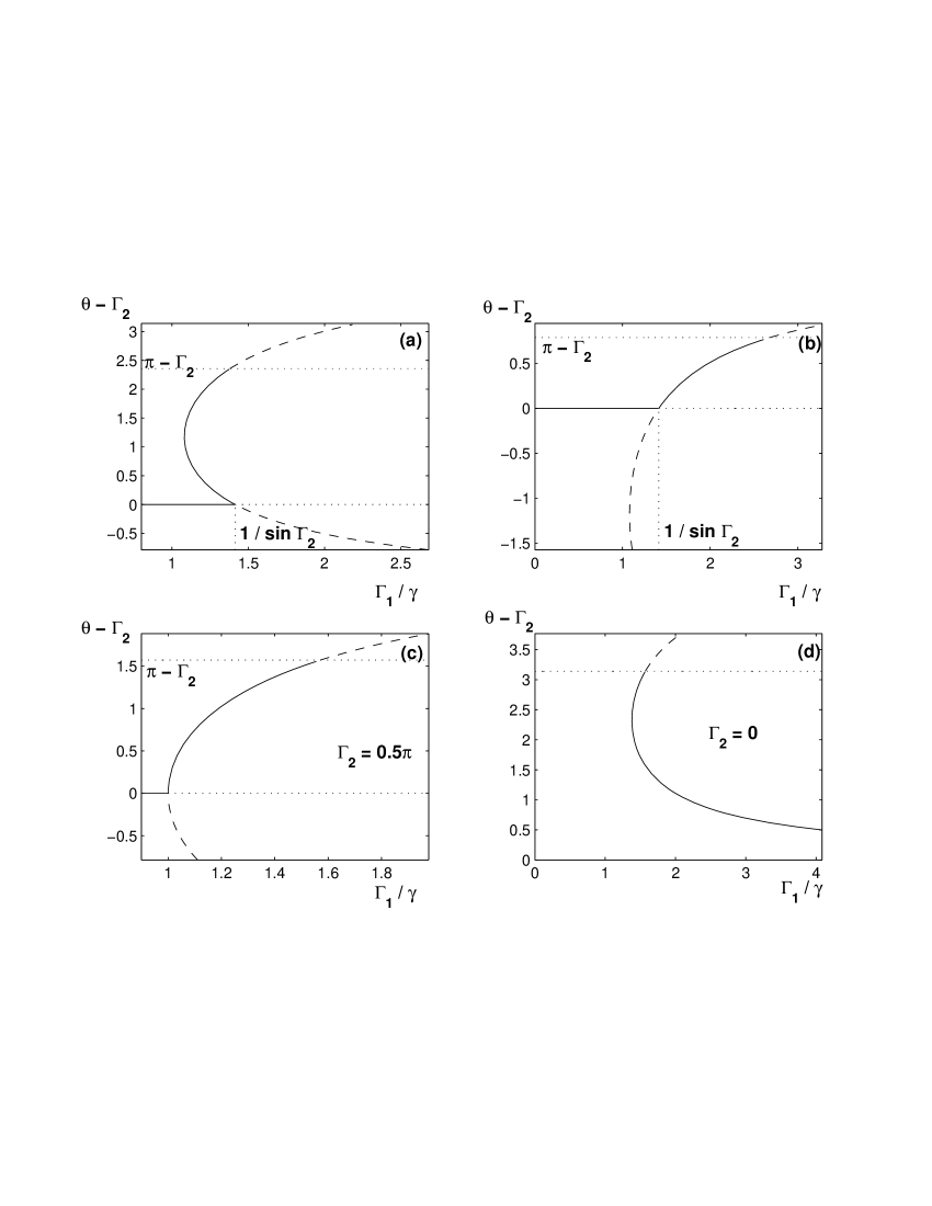
Figure 9: Analytically predicted solution branches for the pinned gap soliton in the BG with weak uniform loss and local gain. Shown is $\theta-\Gamma_{2}$ vs. the gain strength, $\Gamma_{1}/\gamma$. (a) $\Gamma_{2}=\pi/4$; (b) $\Gamma_{2}=3\pi/4$; (c) $\Gamma_{2}=\pi/2$; (d) $\Gamma_{2}=0$. In the last case, nontrivial solutions appear at point $\theta=0.7442\pi,\,\Gamma_{1}/\gamma=1.3801$, and at large values of $\Gamma_{1}/\gamma$ the continuous curve asymptotically approaches the horizontal axis. In all the panels, the dashed lines show a formal continuation of the solutions in the unphysical regions, $\theta<\Gamma_{2}$, and $\theta>\pi$. In panels (a), (b), and (c), the trivial solution, $\theta-\Gamma_{2}=0$, is shown by the solid line where it is stable; in the case corresponding to the panel (d), all the axis $\theta=0$ corresponds to the stable trivial solution.

IV.3 Stability of the zero solution

As done above for the CGLE model with the HS, see Eqs. (50) - (52), it is relevant to analyze the stability of the zero background, and the relation between the onset of the localized instability, driven by the HS, and the emergence of the stable pinned mode, in the framework of the CMEs. To this end, a solution to the linearized version of the CMEs is looked for as

$$\left\{u(x,z),v(x,z)\right\}=\left\{A_{+},B_{+}\right\}e^{\Lambda z-Kx}\,\;\mathrm{at}\;x>0,$$

$$\left\{u(x,z),v(x,z)\right\}=\left\{A_{-},B_{-}\right\}\,e^{\Lambda z+Kx},\;\mathrm{at}\;x<0,$$

with Re$\{K\}>0$. A straightforward analysis makes it possible to eliminate constant $K$ and find the instability growth rate Mak :

$$\mathrm{Re}\,\Lambda=-\gamma+\left(\sinh\,\Gamma_{1}\right)\,|\sin\,\Gamma_{2}|\,.$$ (80)

Thus, the zero solution is subject to the HS-induced instability, provided that the local gain is strong enough:

$$\sinh\,\Gamma_{1}>\sinh\left(\left(\Gamma_{1}\right)_{\mathrm{cr}}\right)\equiv\gamma/|\sin\,\Gamma_{2}|\,.$$ (81)

Note that the instability is impossible in the absence of the local potential $\sim\Gamma_{2}$. The instability-onset condition (81) simplifies in the limit when both the loss and gain parameters are small (while $\Gamma_{2}$ is not necessarily small):

$$\Gamma_{1}>\left(\Gamma_{1}\right)_{\mathrm{cr}}\approx\gamma/|\sin\,\Gamma_{2}|\,\,.$$ (82)

As seen in Fig. 9, the pinned mode emerges at critical point (82), for $\Gamma_{2}\geq\pi/2$, while at $\Gamma_{2}<\pi/2$ it emerges at $\Gamma_{1}<$ $\left(\Gamma_{1}\right)_{\mathrm{cr}}$.

IV.4 Numerical results

First, direct simulations of the conservative version of CMEs (15), (16), with $\gamma=\Gamma_{1}=0$ (and $\Gamma_{2}>0$) and an appropriate approximation for the delta-function, have demonstrated that there is a very narrow stability interval in terms of parameter $\theta$ [see Eqs. (70)-(74), close to (slightly larger than) $\theta_{\mathrm{stab}}\approx\pi/2$, such that the solitons with $\theta<\theta_{\mathrm{\ stab}}$ decay into radiation, while initially created solitons with $\theta>\theta_{\mathrm{stab}}$ spontaneously evolve, through emission of radiation waves, into a stable one with $\theta\approx\theta_{\mathrm{stab}}$ Mak-earlier ; Mak . This value weakly depends on $\Gamma_{2}$. For instance, at $\Gamma_{2}=0.1$, the stability interval is limited to $0.49\pi<\theta<0.52\pi$, while at a much larger value of the local-potential strength, $\Gamma_{2}=1.1$, the interval is located between boundaries $0.51\pi<\theta<0.55\pi$. In this connection, it is relevant to mention that in the usual BG model, based on Eqs. (15), (16) with $\Gamma_{2}=0$, the quiescent solitons are stable at $\theta<\theta_{\mathrm{cr}}^{(0)}\approx 1.011\cdot\left(\pi/2\right)$ Barash ; Trillo .

Direct simulations of the full CME system (15), (16), which includes weak loss and local gain, which may be considered as perturbations, produce stable dissipative gap solitons with small but persistent internal oscillations, i.e., these are, strictly speaking, breathers, rather than stationary solitons Mak . An essential finding is that the average value of $\theta$ in such robust states may be essentially larger than the above-mentioned $\theta_{\mathrm{stab}}\approx\pi/2$ selected by the conservative counterpart of the system, see particular examples in Table 1. With the increase of the gain strength $\Gamma_{1}$, the amplitude of the residual oscillations increases, and, eventually, the oscillatory state becomes chaotic, permanently emitting radiation waves, which increases the effective loss rate that must be compensated by the local gain.

Taking values of $\gamma$ and $\Gamma_{1}$ small enough, it was checked if the numerically found solutions are close to those predicted by the perturbation theory in the form of Eqs. (71) and (72), with $\theta$ related to $\gamma$ and $\Gamma_{1}$ as per Eq. (77). It has been found that the quasi-stationary solitons (with the above-mentioned small-amplitude intrinsic oscillations) are indeed close to the analytical prediction. The corresponding values of $\theta$ were identified by means of the best fit to expression (71). Then, for the so found values of $\theta$ and given loss coefficient $\gamma$, the equilibrium gain strength $\Gamma_{1}$ was calculated as predicted by the analytical formula (77), see a summary of the results in Table 1. It is seen in the Table that the numerically found equilibrium values of $\Gamma_{1}$ exceeds the analytically predicted counterparts by $\sim 10\%-15\%$, which may be explained by the additional gain which is necessary to compensate the permanent power loss due to the emission of radiation.

$\gamma$	$\theta$	$\left(\Gamma_{1}\right)_{\mathrm{num}}$	$\left(\Gamma_{1}\right)_{\mathrm{anal}}$	$\frac{\left(\Gamma_{1}\right)_{\mathrm{num}}-\left(\Gamma_{1}\right)_{\mathrm{anal}}}{\left(\Gamma_{1}\right)_{\mathrm{anal}}}$
$0.000316$	$0.5\pi$	$0.000422$	$0.000386$	$0.0944$
$0.00316$	$0.595\pi$	$0.0042$	$0.00369$	$0.1373$
$0.01$	$0.608\pi$	$0.01333$	$0.01165$	$0.1442$
$0.1$	$0.826\pi$	$0.1327$	$0.121$	$0.0967$

Table 1. Values of the loss parameter $\gamma$ at which quasi-stationary stable pinned solitons were found in simulations of the CME system, (15), (16), by adjusting gain $\Gamma_{1}$, for fixed $\Gamma_{2}=0.5$. Values of the soliton parameter, $\theta$, which provide for the best fit of the quasi-stationary solitons to the analytical solution (71) are displayed too. $\left(\Gamma_{1}\right)_{\mathrm{anal}}$ is the gain coefficient predicted, for given $\gamma$, $\theta$, and $\Gamma_{2}$, by the energy-balance equation (77), which does not take the radiation loss into account. The rightmost column shows the relative difference between the numerically found and analytically predicted gain strength, which is explained by the necessity to compensate additional radiation loss.

It has also been checked that the presence of nonzero attractive potential with $\Gamma_{2}>0$ is necessary for the stability of the gap solitons pinned to the HS in the BG model. In addition to the analysis of stationary pinned modes, collisions between a gap soliton, freely moving in the weakly lossy medium, with the HS were also studied by means of direct simulations Mak . The collision splits the incident soliton into the transmitted and trapped components.

V Discrete solitons pinned to the hot spot in the lossy lattice

The 1D version of the discrete model based on Eq. (21), i.e.,

$$\frac{du_{n}}{dz}=\frac{i}{2}\left(u_{n-1}+u_{n+1}+u_{n-1}-2u_{m,n}\right)$$

$$-\gamma u_{n}+\left[\left(\Gamma_{1}+i\Gamma_{2}\right)+\left(iB-E\right)|u_{n}|^{2}\right]\delta_{n,0}u_{n},$$ (83)

makes it possible to gain insight into the structure of lattice solitons supported by the “hot site”, at which both the gain and nonlinearity are applied, as in that case an analytical solution is available we . It is relevant to stress that the present model admits stable localized states even in the case of the unsaturated cubic gain, $E<0$, see details below.

V.1 Analytical results

The known staggering transformation review ; PGK , $u_{m}(t)\equiv\left(-1\right)^{m}e^{-2it}\tilde{u}_{m}^{\ast}$, where the asterisk stands for the complex conjugate, reverses the signs of $\Gamma_{2}$ and $B$ in Eq. (83). Using this option, the signs are fixed by setting $\Gamma_{2}>0$ (the linear discrete potential is attractive), while $B=+1$ or $B=-1$ corresponds to the SF and SDF nonlinearity, respectively. Separately considered is the case of $B=0$, when the nonlinearity is represented solely by the cubic dissipation localized at the HS.

Dissipative solitons with real propagation constant $k$ are looked for by the substitution of $u_{m}=U_{m}e^{ikz}\$in Eq. (83). Outside of the HS site, $m=0$, the linear lattice gives rise to the exact solution with real amplitude $A$,

$$U_{m}=A\exp(-\lambda|m|),\;|m|~{}\geq 1,$$ (84)

and complex $\lambda\equiv\lambda_{1}+i\lambda_{2}$, localized modes corresponding to $\lambda_{1}>0$. The analysis demonstrates that the amplitude at the HS coincides with $A$, i.e., $U_{0}=A$. Then, the remaining equations at $n=0$ and $n=1$ yield a system of four equations for four unknowns, $A$, $\lambda_{1}$, $\lambda_{2}$, and $k$:

$$-1+\cosh\lambda_{1}\cos\lambda_{2}=k,~{}-\gamma-\sinh\lambda_{1}\sin\lambda_{2}=0,$$

$$e^{-\lambda_{1}}\sin\lambda_{2}-\gamma+\Gamma_{1}-EA^{2}=0,$$

$$e^{-\lambda_{1}}\cos\lambda_{2}-1+\Gamma_{2}+BA^{2}=k.$$ (85)

This system was solved numerically. The stability of the discrete SDSs was analyzed by the computation of eigenvalues for modes of small perturbations PGK ; Yang and verified by means of simulations of the perturbed evolution. Examples of stable discrete solitons can be seen below in Fig. 12.

In the linear version of the model, with $B=E=0$ in Eq. (83), amplitude $A$ is arbitrary, dropping out from Eqs. (85). In this case, $\Gamma_{1}$ may be considered as another unknown, determined by the balance between the background loss and localized gain, which implies structural instability of the stationary trapped modes in the linear model against small variations of $\Gamma_{1}$. In the presence of the nonlinearity, the power balance is adjusted through the value of the amplitude at given $\Gamma_{1}$, therefore solutions can be found in a range of values of $\Gamma_{1}$. Thus, families of pinned modes can be studied, using linear gain $\Gamma_{1}$ and cubic gain/loss $E$ as control parameters (in the underlying photonic lattice, their values may be adjusted by varying the intensity of the external pump).

V.2 Numerical results

V.2.1 The self-defocusing regime ($B=-1$)

The most interesting results were obtained for the unsaturated nonlinear gain, i.e., $E<0$ in Eq. (83). Figure 10 shows amplitude $A$ of the stable (solid) and unstable (dashed) pinned modes as a function of linear gain $\Gamma_{1}>0$ and cubic gain. The existence of stable subfamilies in this case is a noteworthy finding. In particular, at $E=0$ there exists a family of stable pinned modes in the region of $0.73\leq\Gamma_{1}\leq 1.11$, with the amplitude ranging from $A=0.08$ to $A=0.89$. Outside this region, solutions decay to zero if the linear gain is too weak ($\Gamma_{1}<0.73$), or blow up at $\Gamma_{1}>1.11$. Figure 10 shows that the bifurcation of the zero solution $A=0$ into the pinned mode takes place at a particular value $\Gamma_{1}=0.7286$, which is selected by the above-mentioned power-balance condition in the linear system.

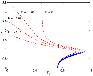
Figure 10: (Color online) Amplitude $A$ of the pinned 1D discrete soliton as a function of linear ($\Gamma_{1}$) and cubic ($E\leq 0$) gain. Other parameters in Eq. (83) are $\gamma=0.5$, $\Gamma_{2}=0.8$, and $B=-1$ (the SDF nonlinearity). Here and in Figs. 11 and 13 below, continuous and dashed curves denote stable and unstable solutions, respectively.

The existence of the stable pinned modes in the absence of the gain saturation being a remarkable feature, the stability region is, naturally, much broader in the case of the cubic loss, $E>0$. Figure 11 shows the respective solution branches obtained with the SDF nonlinearity. When the cubic loss is small, e.g., $E=0.01$, there are two distinct families of stable modes, representing broad small-amplitude ($A\leq 0.89$) and narrow large-amplitude ($A\geq 2.11$) ones. These two stable families are linked by an unstable branch with the amplitudes in the interval of $0.89<A<2.11$. The two stable branches coexist in the interval of values of the linear gain $0.73\leq\Gamma_{1}\leq 1.13$, where the system is bistable. Figure 12 shows an example of the coexisting stable modes in the bistability region. In simulations, a localized input evolves into either of these two stable solutions, depending on the initial amplitude.

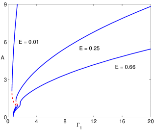
Figure 11: (Color online) Solution branches for the discrete solitons in the case of the cubic loss ($E>0$) and SDF nonlinearity ($B=-1$). The other parameters are same as those in Fig. 10.

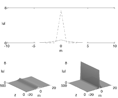
Figure 12: The coexistence of stable small- and large-amplitude pinned discrete modes (top), and the corresponding evolution of nonstationary solutions (bottom) at $E=0.01$, in the bistability region. Inputs with amplitudes $A=0.3$ and $A=2$ evolve into the small-amplitude and large-amplitude stationary modes, respectively. The other parameters are $\gamma=0.5$, $\Gamma_{1}=1$, $\Gamma_{2}=0.8$, and $B=-1$ (the SDF nonlinearity).

While the pinned modes may be stable against small perturbations under the combined action of the self-defocusing nonlinearity ($B=-1$) and unsaturated nonlinear gain ($E\leq 0$), one may expect fragility of these states against finite-amplitude perturbations. It was found indeed that sufficiently strong perturbations destroy those modes we .

V.2.2 The self-focusing regime ($B=+1$)

In the case of the SF nonlinearity, $B=+1$, the pinned-mode branches are shown in Fig. 13, all of them being unstable without the cubic loss, i.e., at $E\leq 0$. For the present parameters, all the solutions originate, in the linear limit, from the power-balance point $\Gamma_{1}=0.73$. The localized modes remain stable even at very large values of $\Gamma_{1}$. Lastly, in the case of $B=0$, when the nonlinearity is represented solely by the cubic gain or loss, all the localized states are unstable under the cubic gain, $E<0$, and stable under the cubic loss, $E>0$.

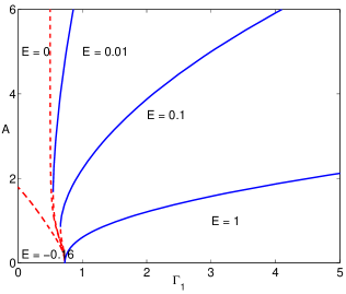
Figure 13: (Color online) Amplitude $A$ of the discrete pinned mode as a function of the linear gain ($\Gamma_{1}$) and cubic loss ($E$) in the case of the SF nonlinearity, $B=+1$. The other parameters are $\gamma=0.5$ and $\Gamma_{2}=0.8$.

VI Conclusion

This article presents a limited review of theoretical results obtained in recently studied 1D and 2D models, which predict a generic method for supporting stable spatial solitons in dissipative optical media, based on the use of the linear gain applied in narrow active segments (HSs, “hot spots”) implanted into the lossy waveguide. In some cases, the unsaturated cubic localized gain may also support stable spatial solitons, which is a counter-intuitive finding. In view of the limited length of the article, it combined a review of the broad class of such models with a more detailed consideration of selected 1D models where exact or approximate analytical solutions for the dissipative solitons are available. Naturally, the analytical solutions, in the combination with their numerical counterparts, provide a deeper understanding of the underlying physical models.

A relevant issue for the further development of the topic is a possibility of the existence of asymmetric modes supported by symmetric double HSs, i.e., the analysis of the spontaneous symmetry breaking in this setting book . Thus far, such a result was not demonstrated in a clear form. Another challenging extension may be a possibility of dragging a pinned 1D or 2D soliton by a HS moving across a lossy medium.

VII Acknowledgement

I appreciate the invitation from Prof. G. Swartzlander, the Editor-in-Chief of J. Opt. Soc. Am. B, to draft and submit this mini-review. My work on the present topic has greatly benefited from collaborations with many colleagues, including P. L. Chu (deceased), N. B. Aleksić, J. Atai, O. V. Borovkova, K. W. Chow, P. Colet, M. C. Cross, E. Ding, R. Driben, W. J. Firth, D. Gomila, Y.-J. He, Y. V. Kartashov, E. Kenig, S. K. Lai, C. K. Lam, H. Leblond, Y. Li, R. Lifshitz, V. E. Lobanov, W. C. K. Mak, A. Marini, T. Mayteevarunyoo, D. Mihalache, A. A. Nepomnyashchy, P. V. Paulau, H. Sakaguchi, V. Skarka, D. V. Skryabin, A. Y. S. Tang, L. Torner, C. H. Tsang, V. A. Vysloukh, P. K. A. Wai, H. G. Winful, F. Ye, and X. Zhang.

References

- (1) N. N. Rosanov, Spatial Hysteresis and Optical Patterns (Springer: Berlin, 2002).
- (2) M. Tlidi and P. Mandel, “Transverse dynamics in cavity nonlinear optics (2000-2003)”, J. Opt. B 6, R60-R75 (2004).
- (3) N. Akhmediev and A. Ankiewicz (Eds.), Dissipative Solitons, Lect. Notes Phys. 661 (Springer, Berlin, 2005).
- (4) N. Lazarides and G. P. Tsironis, “Coupled nonlinear Schrödinger field equations for electromagnetic wave propagation in nonlinear left-handed materials”, Phys. Rev. E 71, 036614 (2005).
- (5) Y. M. Liu, G. Bartal, D. A. Genov, and X. Zhang, “Subwavelength discrete solitons in nonlinear metamaterials”, Phys. Rev. Lett. 99, 153901 (2007).
- (6) E. Feigenbaum and M. Orenstein, “Plasmon-soliton”, Opt. Lett. 32, 674-676 (2007).
- (7) I. R. Gabitov, A. O. Korotkevich, A. I. Maimistov, and J. B. Mcmahon, “Solitary waves in plasmonic Bragg gratings”, Appl. Phys. A 89, 277-281 (2007).
- (8) K. Y. Bliokh, Y. P. Bliokh, and A. Ferrando, “Resonant plasmon-soliton interaction”, Phys. Rev. A 79, 041803 (2009).
- (9) Y.-Y. Lin, R.-K. Lee, and Y. S. Kivshar, “Transverse instability of transverse-magnetic solitons and nonlinear surface plasmons”, Opt. Lett. 34, 2982-2984 (2009).
- (10) A. Marini, D. V. Skryabin, and B. A. Malomed, “Stable spatial plasmon solitons in a dielectric-metal-dielectric geometry with gain and loss”, Opt. Exp. 19, 6616-6622 (2011).
- (11) A. V. Gorbach and D. V. Skryabin, “Spatial solitons in periodic nanostructures”, Phys. Rev. A 79, 053812 (2009).
- (12) F. Ye, D. Mihalache, B. Hu, and N. C. Panoiu, “Subwavelength plasmonic lattice solitons in arrays of metallic nanowires”, Phys. Rev. Lett. 104, 106802 (2010)
- (13) M. C. Cross and P. C. Hohenberg, “Pattern formation outside of equilibrium”, Rev. Mod. Phys. 65, 851-1112 (1993).
- (14) I. S. Aranson and L. Kramer, “The world of the complex Ginzburg-Landau equation”, Rev. Mod. Phys. 74, 99 (2002).
- (15) B. A. Malomed, in: Encyclopedia of Nonlinear Science, p. 157 (ed. by A. Scott; New York, Routledge, 2005).
- (16) P. Kolodner, J. A. Glazier, H. Williams, “Dispersive chaos in one-dimensional traveling-wave convection”, Phys. Rev. Lett. 65, 1579-1582 (1990).
- (17) S. K. Das, S. Puri, and M. C. Cross, “Nonequilibrium dynamics of the complex Ginzburg-Landau equation: Analytical results”, Phys. Rev. E 64, 046206 (2001).
- (18) L. M. Hocking and K. Stewartson, “Nonlinear response of a marginally unstable plane parallel flow to a 2-dimensional disturbance”, Proc. R. Soc. London Ser. A 326, 289-313 (1972).
- (19) N. R. Pereira, L. Stenflo, “Nonlinear Schrödinger equation including growth and damping”, Phys. Fluids 20,1733-1734 (1977).
- (20) B. A. Malomed and H. G. Winful, “Stable solitons in two-component active systems”, Phys. Rev. E 53, 5365-5368 (1996).
- (21) J. Atai and B. A. Malomed, “Stability and interactions of solitons in two-component active systems”, Phys. Rev. E 54, 4371-4374 (1996).
- (22) J. Atai and B. A. Malomed, “Exact stable pulses in asymmetric linearly coupled Ginzburg–Landau equations”, Phys. Lett. A 246, 412-422 (1998).
- (23) H. Sakaguchi and B. A. Malomed, “Breathing and randomly walking pulses in a semilinear Ginzburg-Landau system” Physica D 147, 273-282 (2000).
- (24) B. A. Malomed, “Solitary pulses in linearly coupled Ginzburg-Landau equations”, Chaos 17, 037117 (2007).
- (25) P. V. Paulau, D. Gomila, P. Colet, N. A. Loiko, N. N. Rosanov, T. Ackemann, and W. J. Firth, “Vortex solitons in lasers with feedback”, Optics Express 18, 8859-8866 (2010).
- (26) P. V. Paulau, D. Gomila, P. Colet, B. A. Malomed, and W. J. Firth, “From one- to two-dimensional solitons in the Ginzburg-Landau model of lasers with frequency-selective feedback”, Phys. Rev. E 84, 036213 (2011).
- (27) R. Driben and B. A. Malomed, “Stability of solitons in parity-time- symmetric couplers”, Opt. Lett. 36, 4323-4325 (2011).
- (28) N. V. Alexeeva, I. V. Barashenkov, A. A. Sukhorukov, and Y. S. Kivshar, “Optical solitons in -symmetric nonlinear couplers with gain and loss”, Phys. Rev. A 85, 063837 (2012).
- (29) V. I. Petviashvili and A. M. Sergeev, “Spiral solitons in active media with excitation thresholds”, Doklady AN SSSR (Sov. Phys. Doklady) 276, 1380-1384 (1984).
- (30) B. A. Malomed, “Evolution of nonsoliton and “quasi-classical” wavetrains in nonlinear Schrödinger and Korteweg-de Vries equations with dissipative perturbations”, Physica D 29, 155-172 (1987).
- (31) W. van Saarloos, and P. Hohenberg, “Pulses and fronts in the complex Ginzburg-Landau equation near a subcritical bifurcation”, Phys. Rev. Lett. 64, 749-752 (1990).
- (32) V. Hakim, P. Jakobsen, and Y. Pomeau, “Fronts vs. solitary waves in nonequilibrium systems. Europhys. Lett. 11, 19 (1990).
- (33) B. A. Malomed, and A. A. Nepomnyashchy, “Kinks and solitons in the generalized Ginzburg-Landau equation”, Phys. Rev. A 42, 6009-6014 (1990).
- (34) P. Marcq, H. Chaté, and R. Conte, “Exact solutions of the one-dimensional quintic complex Ginzburg-Landau equation”, Physica D 73, 305-317 (1994).
- (35) T. Kapitula and B. Sandstede, “Instability mechanism for bright solitary-wave solutions to the cubic-quintic Ginzburg-Landau equation”, J. Opt. Soc. Am. B 15, 2757-2762 (1998).
- (36) A. Komarov, H. Leblond, and F. Sanchez, “Quintic complex Ginzburg-Landau model for ring fiber lasers”, Phys. Rev. E 72, 025604(R) (2005).
- (37) W. Renninger, A. Chong, and E. Wise, “Dissipative solitons in normal-dispersion fiber lasers”, Phys. Rev. A 77, 023814 (2008).
- (38) E. Ding and J. N. Kutz, “Operating regimes, split-step modeling, and the Haus master mode-locking model”, J. Opt. Soc. Am. B 26, 2290-2300 (2009).
- (39) J. Hukriede, D. Runde, and D. Kip, “Fabrication and application of holographic Bragg gratings in lithium niobate channel waveguides,” J. Phys. D 36, R1 (2003).
- (40) W. C. K. Mak, B. A. Malomed, and P. L. Chu, “Interaction of a soliton with a localized gain in a fiber Bragg grating”, Phys. Rev. E 67, 026608 (2003).
- (41) C. K. Lam, B. A. Malomed, K. W. Chow, and P. K. A. Wai, “Spatial solitons supported by localized gain in nonlinear optical waveguides”, Eur. Phys. J. Special Topics 173, 233-243 (2009).
- (42) O. V. Borovkova, V. E. Lobanov, and B. A. Malomed, “Stable nonlinear amplification of solitons without gain saturation”, EPL 97, 44003 (2012).
- (43) W. Schöpf and L. Kramer, “Small-amplitude periodic and chaotic solutions of the complex Ginzburg-Landau equation for a subcritical bifurcation”, Phys. Rev. Lett. 66, 2316-2319 (2003).
- (44) D. K. Serkland, G. D. Bartolini, A. Agarwal, P. Kumar, and W. L. Kath, ”Pulsed degenerate optical parametric oscillator based on a nonlinear-fiber Sagnac interferometer”, Opt. Lett. 23, 795-797 (1998).
- (45) M. A. Foster, A. C. Turner, J. E. Sharping, B. S. Schmidt, M. Lipson, A. L. Gaeta, “Broad-band optical parametric gain on a silicon photonic chip,” Nature 441, 960-963 (2006).
- (46) F. Ye, C. Huang, Y. V. Kartashov, and B. A. Malomed, “Solitons supported by localized parametric gain”, Opt. Lett. 38, 480-482 (2013).
- (47) C. H. Tsang, B. A. Malomed, C. K. Lam, and K. W. Chow, “Solitons pinned to hot spots. Eur. Phys. J. D 59, 81-89 (2010).
- (48) D. A. Zezyulin, Y. V. Kartashov, and V. V. Konotop, “Solitons in a medium with linear dissipation and localized gain”, Opt. Lett. 36, 1200-1202 (2011).
- (49) Y. V. Kartashov, Y. V., V. V. Konotop, and V. V. Vysloukh, “Symmetry breaking and multipeaked solitons in inhomogeneous gain landscapes, Phys. Rev. A 83, 041806(R) (2011).
- (50) D. A. Zezyulin, V. V. Konotop, and G. L. Alfimov, “Dissipative double-well potential: Nonlinear stationary and pulsating modes”, Phys. Rev. E 82, 056213 (2010).
- (51) C. H. Tsang, B. A. Malomed, and K. W. Chow, “Multistable dissipative structures pinned to dual hot spots”, Phys. Rev. E 84, 066609 (2011).
- (52) Y. V. Kartashov, V. V. Konotop, and V. V. Vysloukh, “Dissipative surface solitons in periodic structures”, EPL 91, 340003 (2010).
- (53) W. Zhu, Y. He, B. A. Malomed, and D. Mihalache, “Two-dimensional solitons and clusters in dissipative lattices”, J. Opt. Soc. Am. B 31, A1-A5 (2014).
- (54) D. A. Zezyulin, G. L. Alfimov, and V. V. Konotop, “Nonlinear modes in a complex parabolic potential”, Phys. Rev. A 81, 013606 (2010).
- (55) F. K. Abdullaev, V. V. Konotop, M. Salerno,and A. V. Yulin, “Dissipative periodic waves, solitons, and breathers of the nonlinear Schrödinger equation with complex potentials”, Phys. Rev. E 82, 056606 (2010).
- (56) V. Skarka, N. B. Aleksić, H. Leblond, B. A. Malomed, and D. Mihalache, “Varieties of Stable Vortical Solitons in Ginzburg-Landau Media with Radially Inhomogeneous Losses”, Phys. Rev. Lett. 105, 213901 (2010).
- (57) V. E. Lobanov, Y. V. Kartashov, V. A. Vysloukh, and L. Torner, “Stable radially symmetric and azimuthally modulated vortex solitons supported by localized gain”, Opt. Lett. 36, 85-87 (2011).
- (58) O. V. Borovkova, V. E. Lobanov, Y. V. Kartashov, and L. Torner, “Rotating vortex solitons supported by localized gain”, Opt. Lett. 36, 1936-1938 (2011).
- (59) O. V. Borovkova, Y. V. Kartashov, V. E. Lobanov, V. A. Vysloukh, and L. Torner, “Vortex twins and anti-twins supported by multiring gain landscapes”, Opt. Lett. 36, 3783-3785 (2011).
- (60) C. Huang, F. Ye, B. A. Malomed, Y. V. Kartashov, and X. Chen, “Solitary vortices supported by localized parametric gain”, Opt. Lett. 38, 2177-2180 (2013).
- (61) C. Huang, F. Ye, B. A. Malomed, Y. V. Kartashov, and X. Chen, “Solitary vortices supported by localized parametric gain”, Opt. Lett. 38, No. 3, 2177-2179 (2013).
- (62) A. Ruschhaupt, F. Delgado, and J. G. Muga, “Physical realization of -symmetric potential scattering in a planar slab waveguide”, J. Phys. A: Math. Gen. 38, L171-L175 (2005).
- (63) C. E. Rüter,K. G. Makris, R. El-Ganainy, D. N. Christodoulides, M. Segev, and D. Kip, “Observation of parity-time symmetry in optics”, Nat. Phys. 6, 192-195 (2010).
- (64) K. G. Makris, R. El-Ganainy, D. N. Christodoulides, and Z. H. Musslimani, “Beam dynamics in - symmetric optical lattices”, Phys. Rev. Lett. 100, 103904 (2008).
- (65) S. Longhi, “Spectral singularities and Bragg scattering in complex crystals”, Phys. Rev. A 81, 022102 (2010).
- (66) Z. H. Musslimani, K. G. Makris, R. El-Ganainy, and D. N. Christodoulides, “Optical solitons in -periodic potentials”, Phys. Rev. Lett. 100, 030402 (2008).
- (67) Z. Lin, H. Ramezani, T. Eichelkraut, T. Kottos, H. Cao, and D. N. Christodoulides, “Unidirectional invisibility induced by -symmetric periodic structures”, Phys. Rev. Lett. 106, 213901 (2011).
- (68) X. Zhu, H. Wang, L.-X. Zheng, H. Li, and Y.-J. He, Opt. Lett. 36, 2680 (2011).
- (69) S. Nixon, L. Ge, and J. Yang, “Stability analysis for solitons in -symmetric optical lattices”, Phys. Rev. A 85, 023822 (2012).
- (70) H. Cartarius, D. Haag, D. Dast, and G. Wunner, “Nonlinear Schrödinger equation for a -symmetric delta-function double well”, J. Phys. A: Math. Theor. 45, 444008 (2012).
- (71) T. Mayteevarunyoo, B. A. Malomed, and A. Reoksabutr, “Solvable model for solitons pinned to a parity-time-symmetric dipole”, Phys. Rev. E 88, 022919 (2013).
- (72) B. A. Malomed, E. Ding, K. W. Chow, and S. K. Lai, “Pinned modes in lossy lattices with local gain and nonlinearity”, Phys. Rev. E 86, 036608 (2012).
- (73) N. K. Efremidis and D. N. Christodoulides, “Discrete Ginzburg-Landau solitons”, Phys. Rev. E 67, 026606 (2003).
- (74) K. Maruno, A. Ankiewicz, and N. Akhmediev, “Dissipative solitons of the discrete complex cubic-quintic Ginzburg-Landau equation”, Phys. Lett. A 347, 231-240.
- (75) N. K. Efremidis, D. N. Christodoulides,and K. Hizanidis, Two-dimensional discrete Ginzburg-Landau solitons. Phys. Rev. A 76, 043839 (2007).
- (76) N. I. Karachalios, H. E. Nistazakis, and A. N. Yannacopoulos, “Asymptotic behavior of solutions of complex discrete evolution equations: The discrete Ginzburg-Landau equation”, Discrete Contin. Dyn. Syst. 19, 711-736 (2007).
- (77) E. Kenig, B. A. Malomed, M. C. Cross, and R. Lifshitz, “Intrinsic localized modes in parametrically driven arrays of nonlinear resonators”, Phys. Rev. E 80, 046202 (2009).
- (78) C. Mejía-Cortés, J. M. Soto-Crespo, M. I. Molina, and R. A. Vicencio, R. A. “Dissipative vortex solitons in two-dimensional lattices”, Phys. Rev. A 82, 063818 (2010).
- (79) A. Christ, T. Zentgraf, J. Kuhl, S. G. Tikhodeev, N. A. Gippius, and H. Giessen, “Optical properties of planar metallic photonic crystal structures: Experiment and theory, Phys. Rev. B 70, 125113 (2004).
- (80) Y. S. Bian, Z. Zheng, X. Zhao, Y. L. Su, L. Liu, J. S. Liu, J. S. Zhu, and T. Zhou, “Guiding of Long-range hybrid plasmon polariton in a coupled nanowire array at deep-subwavelength scale”, IEEE Phot. Tech. Lett. 24, 1279-1281 (2012).
- (81) B. A. Malomed, E. Ding, K. W. Chow and S. K. Lai, “Pinned modes in lossy lattices with local gain and nonlinearity”, Phys. Rev. E 86, 036608 (2012).
- (82) K. W. Chow, E. Ding, B. A. Malomed, and A. Y. S. Tang, “Symmetric and antisymmetric nonlinear modes supported by dual local gain in lossy lattices”, Eur. Phys. J. Special Topics 223, 63-77 (2014).
- (83) E. Ding, A. Y. S. Tang, K. W. Chow, and B. A. Malomed, “Pinned modes in two-dimensional lossy lattices with local gain and nonlinearity”, Phil. Trans. Roy. Soc. A (in press).
- (84) X. Zhang, J. Chai, J. Huang, Z. Chen, Y. Li, and B. A Malomed, “Discrete solitons and scattering of lattice waves in guiding arrays with a nonlinear -symmetric defect”, Opt. Exp. 22, 13927-13939 (2014).
- (85) V. Skarka, N. B. Aleksić, H. Leblond, B. A. Malomed, and D. Mihalache, “Varieties of stable vortical solitons in Ginzburg-Landau media with radially inhomogeneous losses”, Phys. Rev. Lett. 105, 213901 (2010).
- (86) O. V. Borovkova, Y. V. Kartashov, V. A. Vysloukh, V. E. Lobanov, B. A. Malomed, and L. Torner, “Solitons supported by spatially inhomogeneous nonlinear losses”, Opt. Exp. 20, 2657-2667 (2012).
- (87) G. Iooss and D. D. Joseph, Elementary Stability and Bifurcation Theory (Springer: New York, 1980).
- (88) M. Vakhitov and A. Kolokolov, Radiophys. Quantum. Electron. 16, 783 (1973).
- (89) L. Bergé, Phys. Rep. 303, 259 (1998).
- (90) H. Sakaguchi and B. A. Malomed, “Solitons in combined linear and nonlinear lattice potentials”, Phys. Rev. A 81, 013624 (2010).
- (91) C. M. de Sterke and J. E. Sipe, “Gap solitons”, Progr. Opt. 33, 203-260 (1994).
- (92) D. N. Christodoulides and R. I. Joseph, “Slow Bragg solitons in nonlinear periodic structures” , Phys. Rev. Lett. 62, 1746-1749 (1989).
- (93) A. B. Aceves and S. Wabnitz, “Self-induced transparency solitons in nonlinear refractive periodic media” , Phys. Lett. A 141, 37-42 (1989).
- (94) W. C. K. Mak, B. A. Malomed, and P. L. Chu, “Interaction of a soliton with a local defect in a fiber Bragg grating”, J. Opt. Soc. Am. B 20, 725-735 (2003).
- (95) I. V. Barashenkov, D. E. Pelinovsky, and E. V. Zemlyanaya, “Vibrations and Oscillatory Instabilities of Gap Solitons” , Phys. Rev. Lett. 80, 5117-5120 (1998).
- (96) A. De Rossi, C. Conti, and S. Trillo, “Stability, multistability, and wobbling of optical gap solitons”, Phys. Rev. Lett. 81, 85-88 (1998).
- (97) F. Lederer, G. I. Stegeman, D. N. Christodoulides, G. Assanto, M. Segev, and Y. Silberberg, “Discrete solitons in optics”, Phys. Rep. 463, 1-126 (2008).
- (98) P. G. Kevrekidis, The Discrete Nonlinear Schrödinger Equation: Mathematical Analysis, Numerical Computations, and Physical Perspectives (Springer: Berlin and Heidelberg, 2009).
- (99) J. Yang, Nonlinear Waves in Integrable and Nonintegrable Systems (SIAM: Philadelphia, 2010).
- (100) B. A. Malomed, editor: Spontaneous Symmetry Breaking, Self-Trapping, and Josephson Oscillations (Springer-Verlag: Berlin and Heidelberg, 2013).