Gradient Distribution Priors for Biomedical Image Processing

Abstract

Ill-posed inverse problems are commonplace in biomedical image processing. Their solution typically requires imposing prior knowledge about the latent ground truth. While this regularizes the problem to an extent where it can be solved, it also biases the result toward the expected. With inappropriate priors harming more than they use, it remains unclear what prior to use for a given practical problem. Priors are hence mostly chosen in an ad hoc or empirical fashion. We argue here that the gradient distribution of natural-scene images may provide a versatile and well-founded prior for biomedical images. We provide motivation for this choice from different points of view, and we fully validate the resulting prior for use on biomedical images by showing its stability and correlation with image quality. We then provide a set of simple parametric models for the resulting prior, leading to straightforward (quasi-)convex optimization problems for which we provide efficient solver algorithms. We illustrate the use of the present models and solvers in a variety of common image-processing tasks, including contrast enhancement, noise level estimation, denoising, blind deconvolution, zooming/up-sampling, and dehazing. In all cases we show that the present method leads to results that are comparable to or better than the state of the art; always using the same, simple prior. We conclude by discussing the limitations and possible interpretations of the prior.

1 Introduction

Image processing has become a central element of many workflows in biology and medicine. While the type and source of images varies greatly from light microscopy to magnetic resonance imaging to electron microscopy, the image-processing tasks are often similar. Frequent tasks include image denoising, image deconvolution (beblurring), image zooming (super-resolution), scatter light removal (dehazing), noise level estimation, image quality assessment, and contrast enhancement for image visualization. All of these are inverse problems, as one attempts to reconstruct an unknown “perfect image” from the given imperfect (noisy, blurry, hazy, etc.) observation. Inverse problems are almost always ill-posed or at least ill-conditioned, especially if the transformation that is to be undone is non-linear or unknown.

In order to be able to solve such problems, additional knowledge about the unknown perfect image has to be assumed. Conceptually, there are two approaches to estimating the perfect image: interpolation (smoothing or filtering) and model fitting (Bayesian inference). In the former approach, the additionally assumed knowledge is encoded in the choice of the interpolation method, or in the filter kernels used. These choices typically impose certain geometric properties of the perfect image, such as connectivity, smoothness, sparsity, or curvature. In the Bayesian approach, one attempts to reconstruct a perfect image such that it resembles as much as possible the observed image when run though the (blurring, noise, etc.) transformation. Bayesian inference requires prior knowledge in the form of a prior that sufficiently constrains the reconstruction problem to render it well-posed. Frequently used priors in biomedical image processing include sparsity in the spatial and/or frequency domain [Pustelnik et al., 2011], total variation (TV) [Rudin et al., 1992; Chan et al., 2000; Chantas et al., 2010], mean curvature (MC) [El-Fallah and Ford, 1997; Zhu et al., 2007; Liu et al., 2011], Gaussian curvature (GC) [Lee and Seo, 2005; Zhu et al., 2007; Lu et al., 2011; Gong and Sbalzarini, 2013], and hybrid priors [Kim, 2006; Bredies et al., 2010].

While the prior knowledge regularizes the inverse problem to an extent where it can be solved, it also biases the result toward the expected. It has repeatedly been shown that inappropriate priors may obscure features in the image, or lead to wrong results altogether. Choosing the “right” prior, however, is as hard as solving the original problem, since the underlying perfect image is unknown. The main drawback of frequently used priors is that they bear no relation to the image contents. They merely postulate certain geometric or spectral properties of the image signal, which may mean little. The very popular TV prior [Rudin et al., 1992; Chan et al., 2000; Chantas et al., 2010], for example, presupposes that the unknown perfect image be a collection of uniformly colored or uniformly bright regions, i.e., be piece-wise constant. Imposing this prior leads to removal of image detail and processing artifacts if this presumption is not justified.

Spectral priors have been introduced in order to relax some of the constraints. They do not directly impose knowledge about a property of the perfect image, but only about the histogram (or probability distribution) of that property. As such, they are weaker priors and bias the result less. A particularly popular spectral prior is the Gradient Distribution Prior (GDP), which presupposes a certain statistical distribution of the gradients in the image, i.e., a certain gradient histogram. It has been shown to lead to better results than the TV prior in many image-processing tasks [Zhu and Mumford, 1997; Weiss and Freeman, 2007; Shan et al., 2008; Cho and Lee, 2009; Chen et al., 2010; Krishnan and Fergus, 2009; Cho et al., 2012]. In Section 3, we provide some reasoning about why and when GDP should be preferred. Conceptually, GDPs are related to histogram equalization. However, while the latter presupposes a uniform distribution in the intensity domain, the former operates in the gradient domain, and the presupposed distribution is not uniform, but learned from examples.

Despite their success in signal processing, GDPs learned from natural-scene images have to the best of our knowledge never been adopted in biomedical image processing, nor have they been validated on biomedical images. Validation as a prior entails showing the following two properties:

• Stability: The prior should be independent of the image content. It should be stable against variations in the imaged objects (organs, cells, tissues, etc.) and against different imaging modalities (fluorescence microscopy, electron microscopy, X-ray imaging, etc.). Here, we validate this property for the GDP in Section 5.

• Correlation with image quality: The prior should be correlated with subjectively perceived image quality. Only then, imposing the prior is expected to improve image quality. We show this here for the GDP prior in Section 7.

We provide here a complete validation of the natural-scene GDP for biomedical images. The concept is illustrated in Fig. 1: The GDP is constructed from natural-scene images and is validated on biomedical images. Then, this prior can be used for biomedical image-processing tasks.

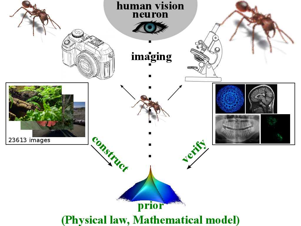
Figure 1: Concept of using natural-scene GDPs in biomedical imaging. The prior is learned from natural-scene images. Since they obey the same physical laws or mathematical model as biomedical images, we propose to use this prior also in that case. We hence learn the GDP from natural-scene images and then validate it on biomedical images, enabling its later application. The human vision system provides the unifying link between the two, as it has evolved to detect and process natural-scene images, but is also used to look at biomedical images.

The second contribution made here is the generalization of GDPs to two (and higher) dimensions, and the introduction of novel parametric models for gradient distributions, which includes the correlation between $x$ and $y$ component. So far, gradient distributions have been modeled under the assumption that the gradient components along $x$ and $y$ are statistically independent in log scale. This, for example, leads to the well-known hyper-Laplacian model Krishnan and Fergus [2009]; Cho et al. [2012]. As we show here, this assumption is not always justified. Often, the gradient components in an image are correlated. Ignoring these correlations may not only lead to artifacts in the result, but also complicates solving the resulting inference problem, frequently requiring alternating optimization over the gradient components. Here, we propose new parametric models for GDP in two dimensions, hence accounting for all correlations. We show that these models not only lead to more accurate results, but also allow simpler and more efficient computational solution of the resulting inference problem. We also highlight the commonalities and differences between the popular TV prior, the hyper Laplace model, and our novel models. In particular, we shown that the popular TV prior can be interpreted as a linear approximation of a GDP in log scale (Section 3.2).

Before presenting our results, however, we formalize the problem in a mathematical framework in Section 2 and provide a detailed motivation of our method in Sections 3 and 4. Stability of the GDP on biomedical images is studied in Section 5. In Section 6 we provide novel parametric models for the GDP in one and two dimensions. Correlation with image quality is shown in Section 7. In Section 8, we demonstrate how to impose the present GDP in a variational framework. In Section 9, we illustrate several applications from biomedical image processing. We conclude and discuss this work in the closing Section 10.

2 Mathematical Framework

We aim at computing an estimate $\hat{U}$ of the unknown, latent perfect image $U(\vec{x})$ from the observed discrete samples $S=\{s_{i}(\vec{x}):i=1\dots N\}$ ($\vec{x}$ is the spatial coordinate), which are the pixels of the data image, or more generally a cloud of data points. The data $S$ have been generated from the underlying truth $U$ by imaging the latter, introducing blur, noise, scattering, down-sampling, etc. This lossy image-formation process is generally modeled as a non-linear map $S=F(U)$. The reconstruction problem can then be expressed in variational form as:

$$\hat{U}=\arg\min_{U^{\prime}\in F_{s}}\left\{\int_{\vec{x}\in\Omega}\!\!\!\Phi_{1}(U^{\prime},S)\,\mathrm{d}\vec{x}+\lambda\!\!\int_{\vec{x}\in\Omega}\!\!\!\Phi_{2}(U^{\prime})\,\mathrm{d}\vec{x}\right\}\,,$$ (1)

where $\Phi_{1}$ is a data-fitting cost function, measuring how well the estimated image approximates the observed image when run through the transformation considered. $\Phi_{1}$ hence models the (generally unknown) imaging transformation $F$. $\Phi_{2}$ constitutes the prior, i.e., a regularization function on $U$. It is common to include a scalar weighting coefficient $\lambda$, called the regularization coefficient, which tunes the trade-off between the data and the prior. The optimal value of $\lambda$ is only known for certain special models (Section 3.2). $\Omega$ is the image domain, and $F_{s}$ is the postulated function space in which $U$ lives.

The choice of function space $F_{s}$ (e.g., $C^{2}(\Omega)$, $C^{4}(\Omega)$, or Bounded Variation space over $\Omega$) defines the image model. All solutions of the reconstruction problem are members of this space. A popular choice is the space $L^{q}(\Omega)$ ($0\leq q\leq\infty$). When $\frac{1}{q}+\frac{1}{q^{*}}=1$, $L^{q}(\Omega)$ and $L^{q^{*}}(\Omega)$ are dual spaces. From the Hölder inequality, one concludes that $L^{q_{+}}(\Omega)\subseteq L^{q}(\Omega)$, for $\forall q_{+}\geq q\geq 1$. This implies that $L^{1}(\Omega)$ is the most general (least restrictive) space among all $L^{q}(\Omega)$.

$\Phi_{1}$ measures how well a certain hypothetical reconstruction $U^{\prime}$ fits the data $S$. This generally involves a model $\hat{F}$ of the unknown image-formation process $F$. This model is typically built from prior knowledge about the optics of the imaging equipment. In order to quantify the distance between $\hat{F}(U^{\prime})$ and $S$, $\Phi_{1}$ uses any metric or semi-metric, such as the Euclidean distance, the Hausdorff distance, an $\ell_{p}$ distance, tangent distance, or a Bregman divergence [Paul et al., 2013]. The choice of the data-fitting function $\Phi_{1}$ depends on how the data were obtained, on the noise type and magnitude, on the tolerated reconstruction error, and on considerations of computational efficiency. The $\ell_{2}$ norm is commonly used because it filters Gaussian noise on the data. Another frequent choice is the $\ell_{1}$ norm, because it filters outliers.

In most of models, $\Phi_{2}$ is a regularization term, such as Tikhonov, the $\ell_{2}$ norm of the gradient, TV, MC, or GC. This term imposes prior knowledge (sparsity, smoothness, etc.) about the unknown perfect image $U$.

2.1 Spectrally Regularized Models

When using a spectrally regularized model, the regularization term does not directly act on $U^{\prime}$, but on a distribution or histogram $p(U^{\prime})$:

$$\begin{split}\hat{U}=\arg\min_{U^{\prime}\in F_{s}}&\left\{\int_{\vec{x}\in\Omega}\!\!\!\Phi_{1}(U^{\prime},S)\,\mathrm{d}\vec{x}\right\}\\ &s.t.~{}~{}p(\mathcal{J}(U^{\prime}))=p^{\mathrm{pr}}_{\mathcal{J}}\,,\end{split}$$ (2)

where $\mathcal{J}$ is a filter (map, feature, differential operator, etc.) and $p^{\mathrm{pr}}_{\mathcal{J}}$ is the corresponding spectral prior. In GDPs, the filter $\mathcal{J}=\nabla$, and $p(\cdot)$ is the gradient distribution.

The spectral constraint can be relaxed by introducing an auxiliary variable $\tilde{U}$ for decoupling:

$$\begin{split}\hat{U}=\arg\min_{U^{\prime}\in F_{s}}&\left\{\int_{\vec{x}\in\Omega}\!\!\!\,\left[\Phi_{1}(U^{\prime},S)+\lambda\Phi_{2}(U^{\prime},\tilde{U})\right]\,\mathrm{d}\vec{x}\right\},\\ &s.t.~{}~{}p(J(\tilde{U}))=p^{\mathrm{pr}}_{J}\,.\end{split}$$ (3)

The type of decoupling is generic to all variational models with hard constraints. It has previously been used, for example, in split-Bregman [Paul et al., 2013], TGV [Bredies et al., 2010], and Hyper-Laplacian [Krishnan and Fergus, 2009] models. From an optimization point of view, Eq. 2 and Eq. 3 are problems with hard and soft constraint, respectively (details see Section 8).

3 Motivation: Why the Gradient Distribution?

Rather than postulating ad hoc properties of the perfect image to be reconstructed, spectral priors are typically learned or identified from large image collections. Given a sufficiently diverse collection of images, the histogram or probability distribution of a spectral prior is estimated by computing some features over all images. There are many features that can be computed, including color and texture features, but the image gradient is particularly interesting. This is first because it is remarkably stable (invariant) across images. Second, it is easy to compute and can hence be learned from large image collections. Third, the gradient has a simple intuitive meaning as the first-order approximation to the perfect image. Furthermore, reconstructing an image from a given gradient field is computationally simple and efficient. In the following, we use the term gradient field whenever we mean the gradient image, i.e., an image that has the same size as the original data image, but where each pixel stores two values that are the two components of the gradient of the original image at that location. The gradient distribution is the histogram or probability distribution of these values across all pixels, and/or across multiple images. We restrict our discussion to two-dimensional images where the gradient has two components. Extensions to higher-dimensional images are readily possible by adding additional gradient vector components.

GDP have been exploited in Bayesian frameworks for image denoising [Zhu and Mumford, 1997], deblurring [Shan et al., 2008], restoration [Cho et al., 2012], super resolution [Zhang et al., 2012], and others [Weiss and Freeman, 2007; Shan et al., 2008; Cho and Lee, 2009; Chen et al., 2010; Krishnan and Fergus, 2009; Cho et al., 2012]. As shown in Ref. [Cho and Lee, 2009], deblurring in the gradient domain is more efficient than working with the original pixel values [Shan et al., 2008]. This can be explained by the reduced correlation in the gradient domain (cf. Fig. 4), which is favorable for blurring kernel estimation.

It is well known by now that the gradient distribution of any image has a heavy tail in log scale. In previous works, however, the 2D gradient distribution is assumed to be the product of two independent 1D distributions along $x$ and $y$ [Shan et al., 2008; Cho and Lee, 2009; Chen et al., 2010; Krishnan and Fergus, 2009; Cho et al., 2012]. As we show below, this is not necessarily the case and there can be significant correlations between the $x$ and $y$ components of the gradient. The full joint 2D gradient distribution can be estimated from image databases and we provide parametric models for it that enable us to use it similarly to the 1D case.

The gradient distribution has a number of different interpretations that provide additional arguments for its use.

3.1 A statistical argument

Statistical interpretations of images have led to a wealth of powerful reconstruction methods based on Bayesian estimation theory. A very famous example are Markov Random Fields (MRF), as used for example in Fields of Experts models [Roth and Black, 2009; Xu and Wang, 2009; Dong et al., 2012]. They are based on assuming a Gibbs distribution for the pixel intensities $I$:

$$p(I(\vec{x}))=\frac{1}{Z}\prod_{r}\prod_{i=1}^{N}\Psi_{i}((J_{i}*I)_{r};\alpha_{i})\,.$$ (4)

$Z$ is a normalization constant, $J_{i}$ is a linear filter, $*$ is the convolution operator, $r$ a local window size, and $\Psi_{i}$ is modeled as a heavy-tailed (often Student-T) distribution with parameter $\alpha_{i}$ (the number of degrees of freedom). The perfect image is then estimated by a Bayesian Maximum A Posteriori (MAP) estimator. These models are powerful and can learn structural information, but there are several crucial parameters to be tuned: the image filter $J$, the shape of the potential function $\Psi$, the local window size $r$, etc. Of these, the window size $r$ is particularly hard to choose for training and inference.

While MRFs estimate the intensity in each pixel (hence taking a microscopic view of the image), spectral priors describe a global property of the whole image (macroscopic view), ignoring local geometry variations. This leads to more stable estimators from a statistical point of view.

According to Boltzmann, the microscopic and the macroscopic view are connected through the concept of entropy. Interpreting each pixel as a random variable, an image can be seen as a state of a high-dimensional random process (pixels). This corresponds to an Ising model in statistical mechanics. Assuming that of all possible combinations of pixel values one could form, meaningful images are equilibrium states, i.e., states (pixel value combinations) of largest probability, the entropy of the image should also be largest. This is the basis of well-known maximum-entropy estimators, which have proven powerful in machine learning and image processing Gull and Daniell [1978]; Gull and Skilling [1984]; Hu and Li [1991]. Conversely, minimizing the entropy leads to a more structured system, which is also useful in image processing [Awate and Whitaker, 2006]. However, it is clear that simply maximizing the entropy does not only enhance the signal, but also the noise, while simply minimizing the entropy does not only reduce the noise, but also removes image detail. Therefore, a prior is again needed to trade this off. The entropy distribution of natural-scene images is shown in Fig. 2, which suggests that entropy should be kept on a certain level. GDPs achieve exactly this, as shown in Section 6.4.

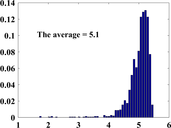
Figure 2: Entropy distribution of natural-scene images.

A simple comparison of point-wise MRFs, Fields-Of-Experts, and GDP is shown in Fig. 3. The figure shows images that were directly sampled from the different prior models. It is worth noticing the unique texture and structure of each model. The main difference comes from the gradient distribution being a macroscopic image description, whereas the other two are microscopic models.

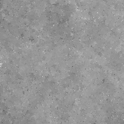
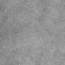
(a) Images generated by a point-wise Markov Random Field.

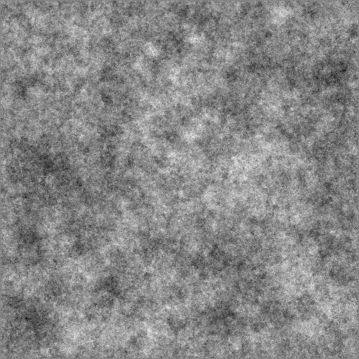
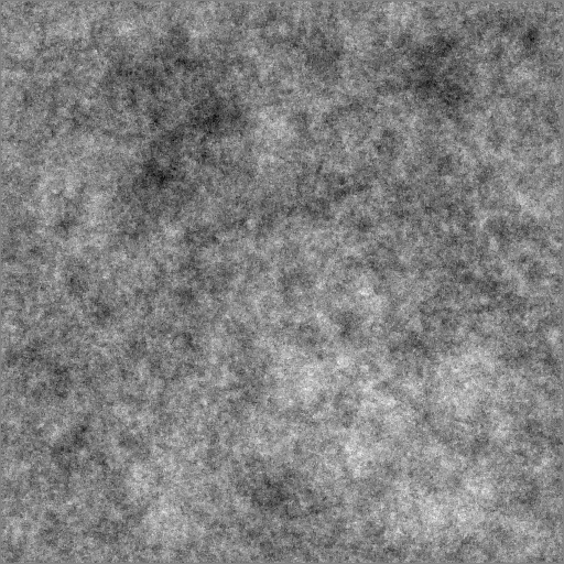
(b) Images generated by a gradient distribution prior.

(c) Images generated by a 3x3 Fields-Of-Experts.

Figure 3: Comparing images sampled from different prior models.

3.2 A variational calculus argument

MAP estimation using Bayes’ rule is equivalent minimizing the negative log-likelihood:

$$\begin{split}\hat{U}=&\arg\max_{U^{\prime}}\ \{\ p(U^{\prime}|S)\propto p(S|U^{\prime})p(U^{\prime})\ \}\\ \Leftrightarrow&\arg\min_{U^{\prime}}\ \{\ -\log(p(S|U^{\prime}))-\lambda\log(p(U^{\prime}))\ \},\end{split}$$ (5)

where the scalar regularization parameter $\lambda$ is introduced to balance the likelihood $p(S|U^{\prime})$ and the prior $p(U^{\prime})$. Assuming a Gaussian distribution for the likelihood naturally leads to an $\ell_{2}$ norm in the data fitting term and to an optimal $\lambda\propto\sigma^{2}$, where $\sigma$ is the standard deviation of the Gaussian.

When using GDP, the prior $p(U^{\prime})$ is not over the hypothetical image $U^{\prime}$, but over its gradient $\nabla U^{\prime}$. A frequent assumption for this term is a Generalized Gaussian distribution, hence $p(\nabla U^{\prime})=\exp^{-\alpha\|\nabla U^{\prime}\|_{*}}$, where $\|\cdot\|_{*}$ is any proper norm. In the negative logarithm, this then leads to the TV regularization $-\log(p(\nabla U^{\prime}))=\alpha\|\nabla U^{\prime}\|_{1}$ for the $\ell_{1}$ norm, corresponding to a Laplace distribution model. The TV regularizer, or the Laplacian model, can hence be interpreted as a linear approximation in log-space to the GDP. This is also visually shown in Fig. 15(h,k). A hyper-Laplacian prior can be imposed in the same way for the $\ell_{q}$ norm ($0<q<1$) [Krishnan and Fergus, 2009].

While MAP uses the posterior as an objective function, other choices are possible. When using the Minimum Mean-Squared Error (MMSE)

$$\hat{U}=\arg\min_{U^{\prime}}\int_{U}^{\prime}p(U^{\prime}|S)U^{\prime}\mathrm{d}U^{\prime}\,.$$ (6)

as a cost function, for example, the prior is imposed analogously. This has been successfully used in conjunction with a TV prior to reduce staircasing artifacts [Louchet and Moisan, 2013]. As shown here in Section 9.3, our GDP model achieves similar results without making the objective function more complex.

3.3 A functional analysis argument

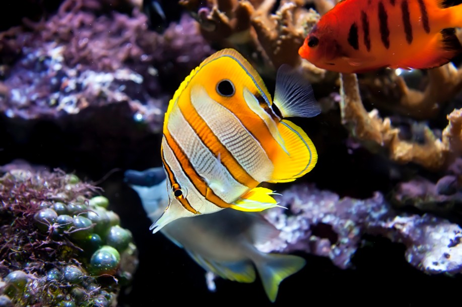
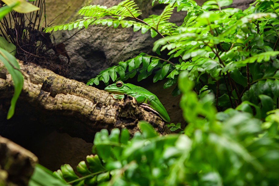
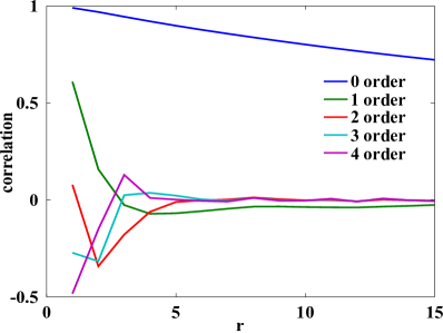
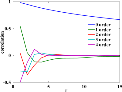
Figure 4: Two example images and their auto-correlation $AC(d,r)$.

According to Taylor’s theorem, the gradient is the first-order approximation to the perfect image. Higher-order approximations, however, do not necessarily improve the accuracy in image processing. The first reason for this is that the discrete image might not be high-order differentiable. A second reason is that the image auto-correlation decreases rapidly with increasing order of derivative. In Fig. 4, the auto-correlation between $I(\vec{x})$ and $I(\vec{x}+\vec{r})$ is shown for different orders $d$ of derivatives:

$$AC(d,r)=\text{correlation}(\nabla^{d}I(\vec{x}),\nabla^{d}I(\vec{x}+\vec{r}))\,,$$ (7)

where $\vec{r}=(r,0)$. The correlation reduces significantly for $d>0$. This explains why gradient and curvature priors are so powerful for image processing, but higher-oder derivatives don’t improve the result anymore. As seen in Fig. 4, the correlation reduces to zero more rapidly for higher $d$. For image-processing tasks, second order has repeatedly been shown to be enough [Zhu et al., 2007; Gong and Sbalzarini, 2013].

An alternative to using image derivatives could be to use Sobolev norms, which implicitly contain gradient information [Sundaramoorthi et al., 2007]. This would mean that $F_{s}$ is a Sobolev space instead of $L^{p}(\Omega)$. When using Sobolev norms, however, there is no way to trade off the weight of the gradient information versus the data. This is why we prefer using GDPs instead of Sobolev norms, because the relative weight is an important parameters allowing us to control the noise level.

3.4 A psychophysical argument

The human vision system mainly detects gradient information [Chichilnisky, 2001; Pillow et al., 2005; Cao et al., 2011; Gollisch and Meister, ]. As shown in Fig. 5, light entering the retina first arrives at the retinal ganglion cells. These cells are sensitive to gradient information, rather than to intensity, with a response that is described well by the error function [Chichilnisky, 2001; Miller and Troyer, 2002]. Neighboring cells also interact with each other to amplify the gradient information, which explains the famous Mach band effect.

During evolution, the neurons have adapted to the environment they were exposed to, and to process what is expected [Chichilnisky, 2001; Simoncelli and Olshausen, 2001; Miller and Troyer, 2002]. This is the gradient distribution found in natural-scene images. The human vision systems is hence particularly well adapted to detect and process images that satisfy this distribution.

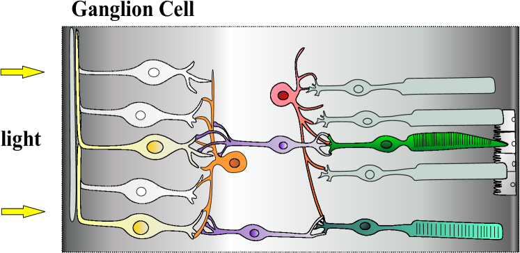
Figure 5: Structure of the human retina. Light first hits the gradient detectors.

The fact that different people have almost the same visual perception is a consequence of the stability of the neuronal response to the gradient distribution. The vision system also suggests that coding an image by its gradient is an efficient way (sparse representation). We show coding efficiency and sparsity for the GDP in Section 6.4.

3.5 Gradient field and original image

Regardless of the stability of the gradient distribution, reconstructing an image from its gradient field is accurate and simple, as it constitutes an integration task with one point constraint [Fattal et al., 2002; Pérez et al., 2003; Agrawal and Raskar, 2007; Bhat et al., 2010; Kazhdan et al., 2006; Xu et al., 2011; Gong et al., 2012; Guillemot et al., 2012]. An excellent review about signal processing in the gradient domain can be found in Ref. [Agrawal and Raskar, 2007]. Some recent advances in this area are described in Refs. [Xu et al., 2011, 2012; Fattal, 2009; Farbman et al., 2008; McCann and Pollard, 2008].

Reconstructing an image from its gradient field can be done by solving a Poisson equation. With proper boundary conditions, the solution is unique, and there exists a wealth of stable, efficient, and accurate numerical solvers for this equation (details in Section. 8.1.2).

4 Why not directly learn GDP from biomedical images?

Why are we proposing to learn the GDP from natural-scene images and then apply it to biomedical images (see Fig. 1)? Would it not be better to directly learn the GDP on biomedical images, for which its use is intended? The reason is two-fold: (1) biomedical images contain a variety of disturbances, such as noise, blur, and scattering. If the GDP is later to be used for denoising, deblurring, or dehazing, it must be estimated from images that do not already contain these disturbances. (2) Even if the disturbances should be part of the prior, it is not easy to learn a GDP directly from biomedical images. The main reason is that biomedical images are usually quite noisy, hampering gradient estimation (derivatives amplify noise). Therefore, it is important that the GDP is estimated from “clean” images. We here propose to learn the GDP from natural-scene images. The motivations have been given above. In the following, we fully validate the use of this prior for biomedical images. The few examples in Fig. 6 are to illustrate that natural-scene and biomedical images have at least qualitatively similar gradient distributions.

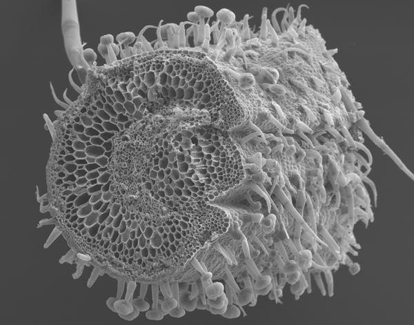
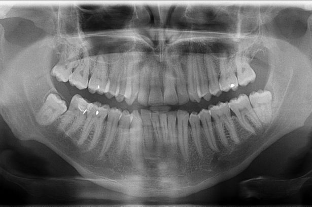
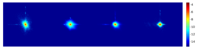
Figure 6: Natural-scene and biomedical images have qualitatively similar gradient distributions and can hence be fitted with the same model. First row: natural-scene image (left) and biomedical images. Second row: corresponding gradient distributions in log scale.

5 The Gradient Distribution Prior (GDP)

In order to build the GDP, we learn the gradient distribution from a database of 23 613 images of natural scenes. We analyze the resulting distributions and compute the variability of images around the mean distribution. We then validate the stability of the GDP on biomedical images.

5.1 Datasets

We collected seven datasets of natural-scene images as shown in Table 1. Each image $I(x,y)$ was converted to 8-bit gray-scale. The gradient field is defined as:

$$\vec{G}(x,y)=\nabla I(x,y),$$ (8)

where here we use the first-order finite difference approximations $\nabla I\approx(I(x+1,y)-I(x,y),I(x,y+1)-I(x,y))$. We use homogeneous Dirichlet boundary conditions at the image borders. Due to the use of 8-bit gray-scale images, possible gradients are in the discrete domain $[-255,255]\times[-255,255]$, where we can easily construct the 2D histogram of $\vec{G}$. We use $G^{x}$ and $G^{y}$ to denote respective components of $\vec{G}$.

In order to turn the histogram into a probability distribution, we divide all bins by the total number of pixels in the image, i.e., by $mn$ where $m$ and $n$ are the number of pixels along the $x$ and $y$ edges of the image. After aggregating data from all images in the database, we further normalize by the total number of images in the dataset. The resulting empirical distribution $p^{\mathrm{pr}}$ is shown in Fig. 7.

Footnote								all
#images	1005	1000	5063	832	1491	6033	8189	23613

Table 1: Natural-scene image datasets used to learn the prior. Source URLs are given in the footnotes.

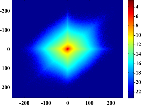
Figure 7: Average gradient distribution of natural-scene images shown in log scale.

5.2 Stability of the prior for natural-scene images

We analyze how closely the natural-scene images in the training dataset match the average gradient distribution learned from them. Fig. 8 shows the histograms of several distances between the average prior and each image’s individual gradient distribution. More than $95\%$ of the images have distributions that are closer to the prior than an RMS of $2\times 10^{-4}$. Also when using other distance metrics, such as the Hellinger or KL distance, the training data are clustered around the prior (Fig. 8b,c).

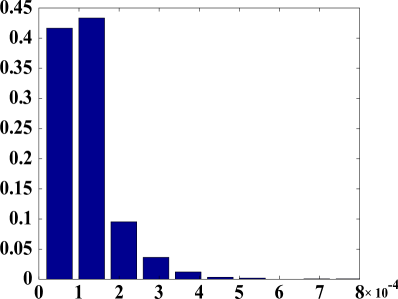
(a) RMS distance

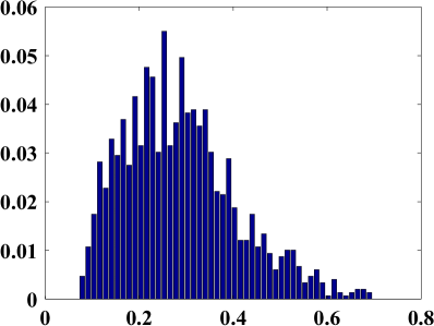
(b) Hellinger distance

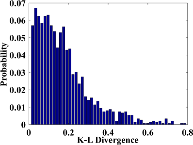
(c) KL distance

Figure 8: The prior is stable across natural-scene images. The distances (different metrics shown) between individual images and the average prior are mostly small, indicating that all images are clustered around the prior.

5.3 Scale stability of the prior

In order for the GDP to be stable across images, it in particular has to be stable with respect to image scaling. We confirm this by down-sampling (down-scaling) all images in the training database by factors up to 0.5, and re-learning the average GDP from each scaled dataset. The scaling is applied to the whole image, rather than cropping a sub-image. The resulting average gradient distributions are shown in Fig 9. They are stable with scaling down to a scale factor of 0.5. Below 0.5, the average gradient distribution starts changing.

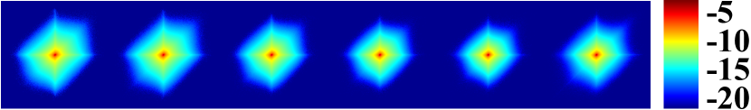
Figure 9: The prior is stable with respect to image scaling. Shown is the average (across the entire training dataset) gradient distribution in log scale for images scaled by factors of (from left to right) 0.5, 0.6, 0.7, 0.8, 0.9, and 1 (i.e., the original, unscaled images).

5.4 Stability of the prior on biomedical images

As mentioned above, it is hard (any potentially undesirable) to directly build a GDP from biomedical images. We hence learned the prior from natural-scene images, but validate it here on biomedical images. We first show stability of the present GDP for biomedical images. For this, we collected a small dataset of biomedical images, including X-ray, MRI, electron microscopy, and fluorescence microscopy images. Some examples are shown in Figs. 10 and 24.

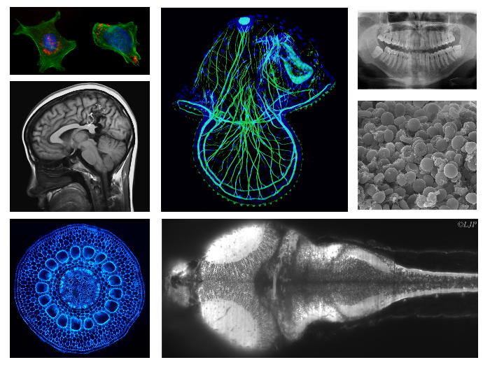
Figure 10: Samples from our biomedical image collection.

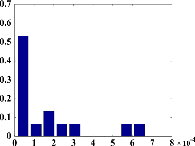
Figure 11: RMS distance from the prior for biomedical images.

We compute the RMS distance from the GDP for each image’s gradient distribution. The distance histogram is shown in Fig. 11. This confirms that most gradient distributions are close to the GDP learned from natural-scene images. As expected, the range of RMS for this test set of biomedical images is larger than the range of RMS for the training set of natural-scene images.

6 Parametric Models for Gradient Distribution Priors

In order to efficiently use the GDP as a regularization term, and to formulate optimization schemed over it, a parametric model is desirable. We here provide two parametric models for the marginal and joint 2D distributions of our GDP, and we assess their approximation accuracy. We compare these new models with traditional gradient distribution models, such as Hyper Laplacian models, and with TV in 1D and 2D. We further propose a new model to approximate the cumulative distribution function (CDF) of the gradient instead of the PDF. This new model only has a single scale parameter, leading to effectively 1D problems in parameter inference. We further discuss the convexity, sparsity, and entropy of these models.

6.1 1D Marginal Model

Traditionally, image gradient distributions are modeled as Generalized Gaussian (Hyper Laplacian) Distributions:

$$\log(P(G^{x}))=-a_{0}|G^{x}|^{b_{0}}+c_{0}\,,$$ (9)

where $a_{0}$, $b_{0}$, and $c_{0}$ are the model parameters. This model includes Gaussian ($b_{0}=2$), Laplacian ($b_{0}=1$), and hyper-Laplacian distributions ($b_{0}=0.6$) [Krishnan and Fergus, 2009] and bears a close relationship with $\ell_{q}$ norms ($0<q<1$).

We instead propose to use the following models for the 1D marginal gradient distribution:

Model 1:

$$\log(P(G^{x}))=2a_{1}\left(\exp\!{\left\{-\frac{|G^{x}|^{b_{1}}}{a_{1}}\right\}}-1\right)+c_{1}(G^{x})^{2}\,,$$ (10)

where $a_{1}$, $b_{1}$, and $c_{1}$ are the parameters. The results of fitting this model (i.e., its parameters) to the average gradient distributions of our image sets are shown in Table 2. To the best of our knowledge, this Model 1 is the best-fitting model known so far (Fig. 14 and Table 3).

Image set		1	2	3	4	5	6	7
$G^{x}$	$a_{1}$	3.66	3.89	3.93	6.51	7.83	5.85	6.34
	$b_{1}$	0.58	0.55	0.58	0.44	0.44	0.45	0.50
	$c_{1}\times 10^{4}$	-2.4	-1.2	-1.5	-0.48	-1.9	-0.57	-1.3
	SSE	40.5	43.0	67.7	23.8	34.1	37.9	25.4
	$R^{2}$	0.99	0.99	0.99	0.99	0.99	0.99	0.99
$G^{y}$	$a_{1}$	3.68	3.87	3.84	7.29	7.29	5.55	6.09
	$b_{1}$	0.60	0.55	0.60	0.42	0.46	0.47	0.51
	$c_{1}\times 10^{4}$	-2.2	-1.2	-1.5	-0.42	-1.9	-0.64	-1.3
	SSE	56.8	41.4	90.8	19.9	29.4	32.6	18.5
	$R^{2}$	0.99	0.99	0.99	0.99	0.99	0.99	0.99
correlation		-0.12	-0.23	-0.19	-0.22	-0.12	-0.25	-0.11
(log scale)		0.37	0.31	0.28	0.37	0.17	0.39	0.18

Table 2: Results for fitting the marginal with Model 1 to the average gradient distributions of all image datasets.

Model 2:

$$\log(P(G^{x}))=-a_{2}(G^{x})^{2}-\log(b_{2}+|G^{x}|^{2})+c_{2},$$ (11)

where $a_{2}$, $b_{2}$, and $c_{2}$ are the parameters. The results of fitting this model to the data are shown in Table 3, compared with other models. Model 2 fits the data less well than the above Model 1, but has several advantages:

• Integrability: Model 2 is integrable, which is convenient for use in optimization algorithms and for analytically computing the CDF. Let $T=\sqrt{a_{2}}$, $b_{2}=0$, and $c_{2}=0$, then the CDF of Model 2 is:

  $$\widetilde{C}(G^{x})=-\frac{e^{-(TG^{x})^{2}}}{G^{x}}-T\sqrt{\pi}\,\text{erf}(TG^{x})+H(G^{x}),$$ (12)

  where $H$ is the Heaviside distribution and erf is the error function. As shown in Fig. 14, the CDF version of this model still works when other models become invalid (Gaussian, Laplacian) or hard to integrate (Hyper-Laplacian, Model 1).

• Computational efficiency: Model 2 has a simple mathematical form that can efficiently be evaluated on a computer. The effect is substantial, as shown in Fig 12(a) for the model evaluation, and in Fig 12(b) for evaluating the gradient of the model (e.g., in an optimization loop).

• Optimization efficiency: Model 2 can be written as the difference of two convex functions. Optimization problems involving Model 2 can hence efficiently be solved using D.C. programming, as shown in Section 8.2.

For these properties, we mainly consider Model 2 as a regularization term in Section 9.

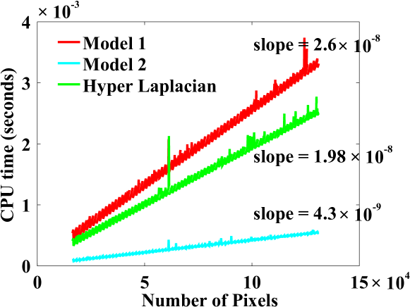
(a) CPU time for evaluating the models.

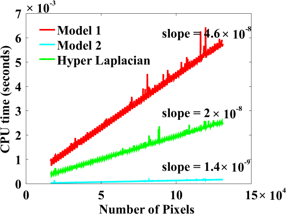
(b) CPU time for evaluating the gradients of the models.

Figure 12: CPU time comparison for model and model gradient evaluations.

We compare our two marginal models with other models in Fig. 14 and Table. 3. In all cases, they outperform the previously used Laplacian, Gaussian, and Hyper-Laplacian models. In Fig. 13, we and analyze the sensitivity of Model 2 as compared with the Hyper-Laplacian model. Model 2 fits the data better and shows good sensitivity (identifiability) with respect to parameter $a_{2}$.

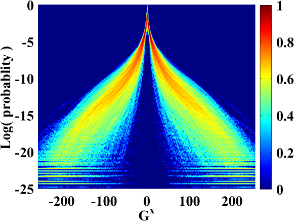
(a) Marginal gradient distribution in log scale for each image. The color indicates scaled density.

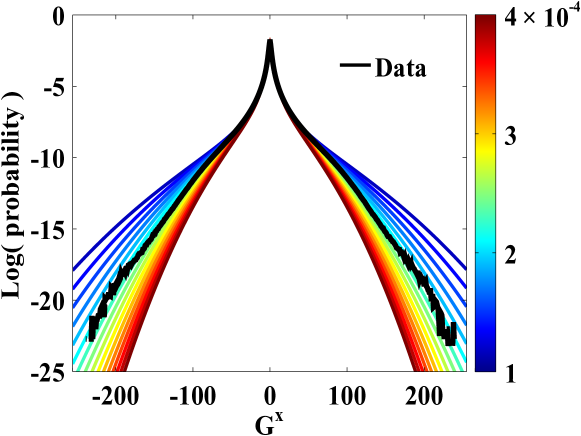
(b) Model 2 with changing parameter $a_{2}$ (coded by color) and other parameters fixed at their best fit: $b_{2}=5.4$, $c_{2}=-0.266$.

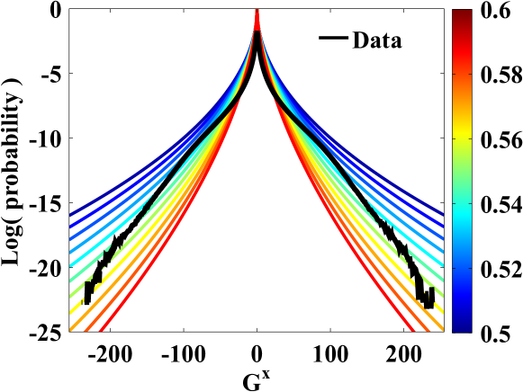
(c) Hyper-Laplacian model with changing parameter $b_{0}$ (color) and all other parameters fixed at their best fit.

Figure 13: Sensitivity analysis of Model 2 compared with the Hyper-Laplacian model. Parameter $a_{2}$ varies from $1\times 10^{-4}$ to $4\times 10^{-4}$ with step size $2\times 10^{-5}$. For the Hyper-Laplacian model, $b_{0}$ varies from 0.5 to 0.6 with step size 0.01.

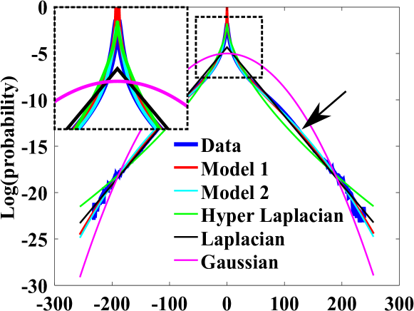
(a) Log scale

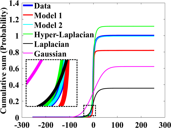
(b) cumulative sum in linear scale

Figure 14: Comparison of marginal models (log scale) and their cumulative sums (linear scale). Optimal parameters are used for each model. The quantitative differences are shown in Table 3; sensitivity analysis of the model fits is shown in Fig. 13.

Image set	1	2	3	4	5	6	7
SSE	40.5	43.0	67.7	23.8	34.1	37.9	25.4
$R^{2}$	0.99	0.99	0.99	0.99	0.99	0.99	0.99
SSE	271	324	266	44.4	38.2	62.8	30.7
$R^{2}$	0.96	0.93	0.96	0.99	0.99	0.98	0.99
SSE	576	301	537	45.4	389	70.5	250
$R^{2}$	0.92	0.93	0.91	0.98	0.96	0.98	0.97
SSE$\times 10^{-3}$	1.86	3.01	3.02	3.95	2.34	3.90	3.95
$R^{2}$	0.74	0.30	0.52	0.13	0.81	0.10	0.57
SSE$\times 10^{-4}$	0.83	1.02	1.10	1.24	1.32	1.23	1.64
$R^{2}$	-0.12	-1.3	-0.72	-2.6	-0.046	-2.5	-0.75

Table 3: Goodness of fit comparison for all models (from top to bottom): Model 1 (Eq. 10), Model 2 (Eq. 11), Hyper-Laplacian, Laplacian, Gaussian.

6.2 2D Joint Model

While the 1D marginal models approximate well the marginal distributions of the gradient, they are not statistically independent. As shown in the last two rows of Table 2, the two gradient components are weakly negatively correlated. This weak correlation between the gradient components explains why alternating optimization had to be used in all previous works that considered the marginal models independently, and why the results were still good even though the prior is not strictly correct.

The traditional model (Eq. 9) can easily be extended to 2D:

$$\log(P(\vec{G}))=-a_{0}(|G^{x}|^{b_{0}}+|G^{y}|^{b_{0}})+c_{0}\,,$$ (13)

where $a_{0}$, $b_{0}$, and $c_{0}$ are the parameters. Such a model, including the Hyper Laplacian as a special case, however, treats the $x$ and $y$ components of the gradient as independent.

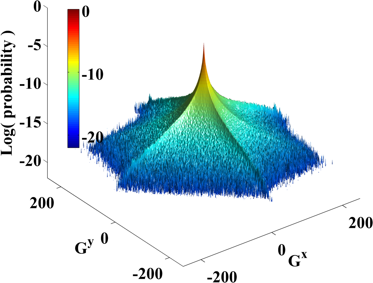
(a) data

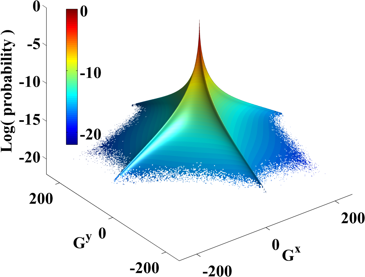
(b) Model 1

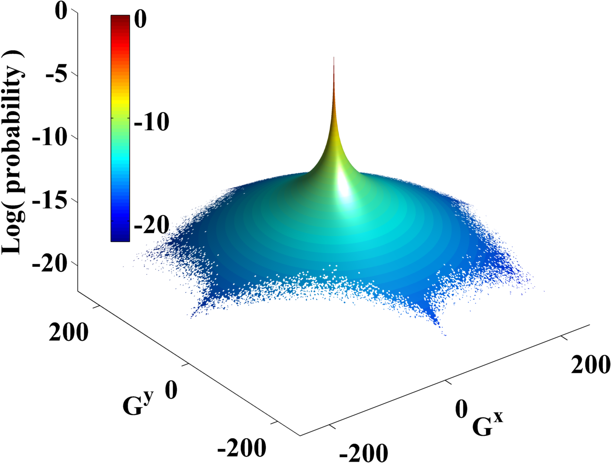
(c) Model 2

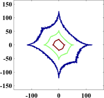
(d) data iso lines

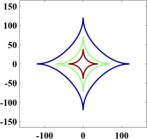
(e) Model 1 iso lines

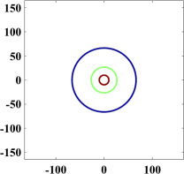
(f) Model 2 iso lines

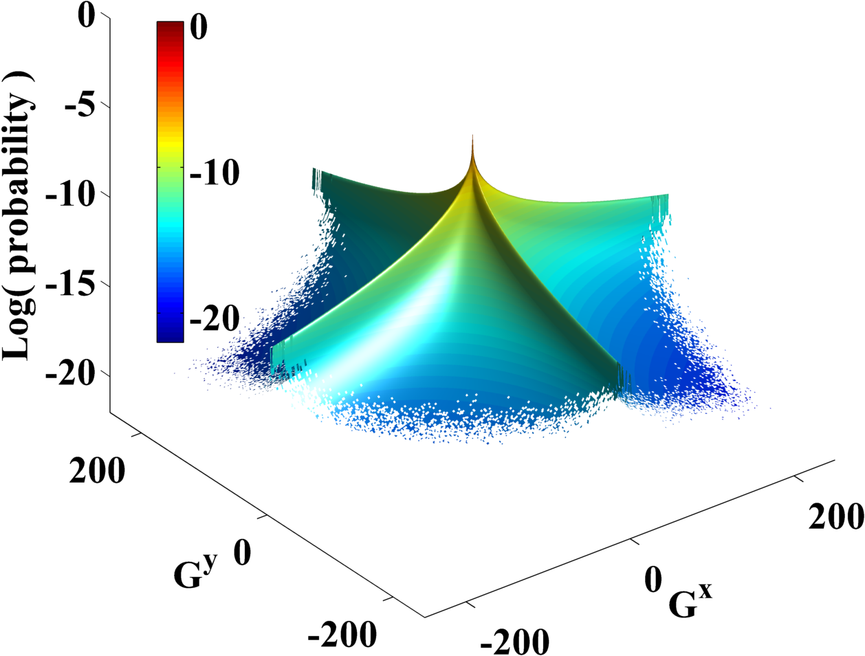
(g) Hyper Laplacian

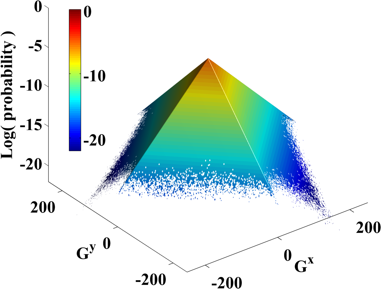
(h) Laplacian

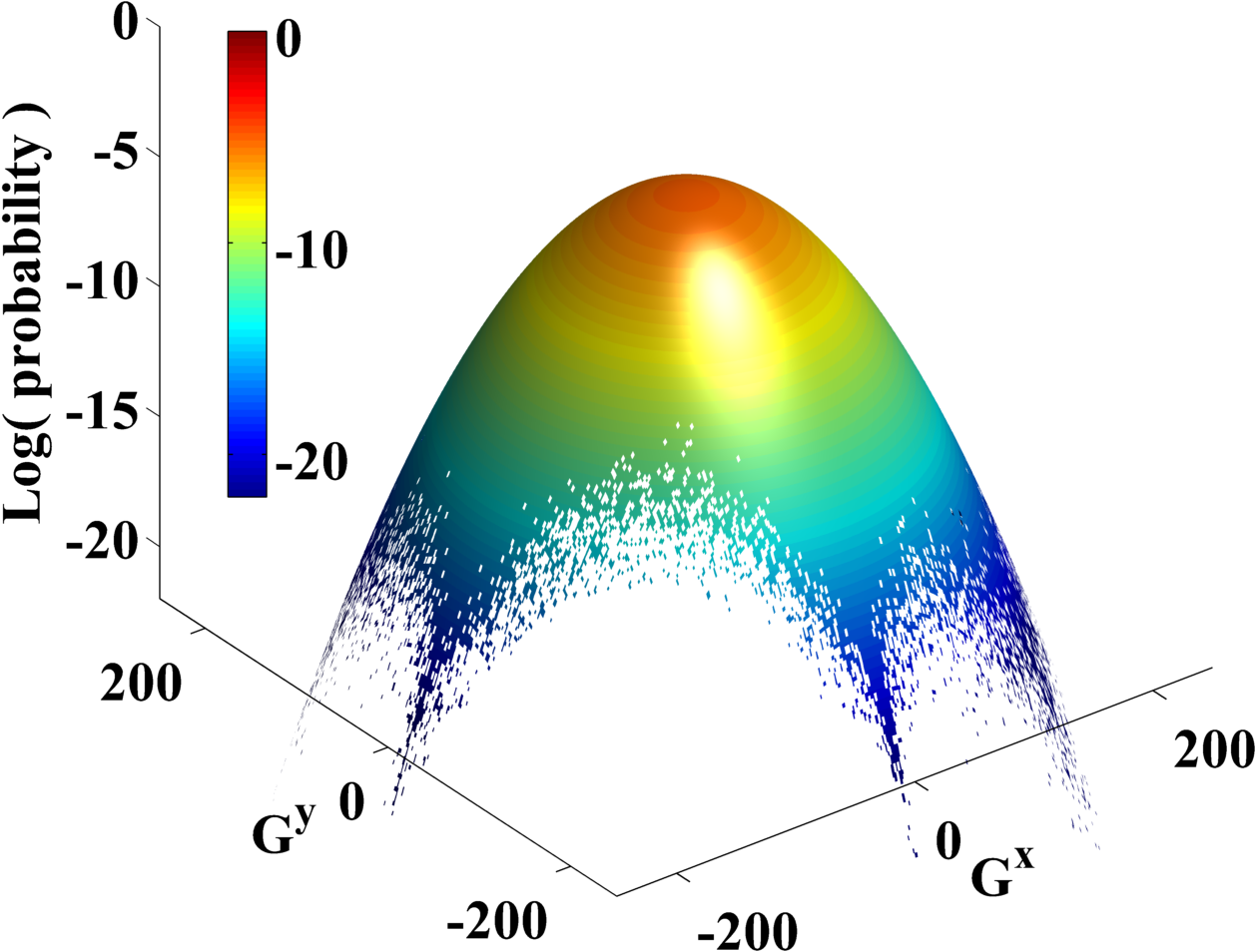
(i) Gaussian

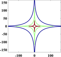
(j) HypLap iso lines

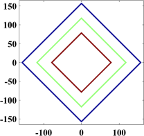
(k) Laplace iso lines

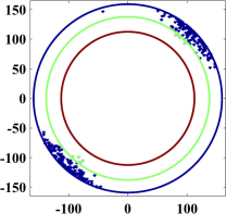
(l) Gaussian iso lines

Figure 15: Visual comparison of model fits for 2D joint gradient distribution models in log scale. First row: 2D gradient distribution of the data followed by plots of the best-fitting 2D models. Second row: iso contours of values -13, -11, and -9. The area included by isoline -13 of Model 2 is only $3\%$ of the whole domain, but the total probability mass in that area is $99\%$. More details about model sparsity are given in Section 6.4.

Considering that a correlation between the gradient components may exist, we instead propose the following two models (corresponding to Model 1 and Model 2 above) for the 2D joint gradient distribution:

$$\log(P)=2a_{1}(\exp\!\left\{{-\frac{|G^{x}|^{b_{1}}+|G^{y}|^{b_{1}}}{a_{1}}}\right\}-1)+c_{1}\lVert\vec{G}\rVert_{2}^{2}\,.$$ (14)

$$\log(P)=-a_{2}(|G^{x}|^{2}+|G^{y}|^{2})-\log(b_{2}+|G^{x}|^{2}+|G^{y}|^{2})+c_{2}\,.$$ (15)

The fitted parameters and are shown in Table 4. Figure 15 compares the model fits with previous models. The data histogram is shown in the left panel of Fig. 15, whereas the best-fit parametric models are plotted in the remaining panels. The area included by isoline -13 of Model 2 is only $3\%$ of the whole domain, but the total probability mass in that area is $99\%$. More details about model sparsity are given in Section 6.4. From Table. 4, it is clear that Eq. 15 fits the data almost as good as Eq. 14, and both models fits much better than any previous model.

(a) original image

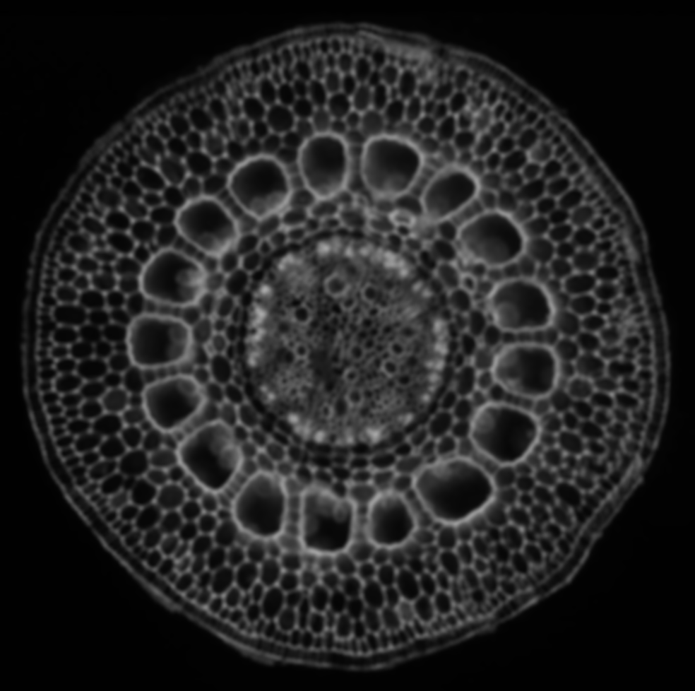
(b) blurred

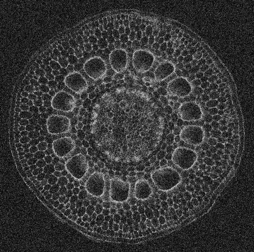
(c) with noise

(d) SR(nearest)

(e) SR(bicubic)

(f) bilateral filter

(g) guided filter

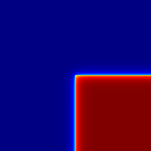
(h) CDF($T$=0.40)

(i) CDF($T$=0.72)

(j) CDF($T$=0.03)

(k) CDF($T$=0.84)

(l) CDF($T$=0.80)

(m) CDF($T$=0.60)

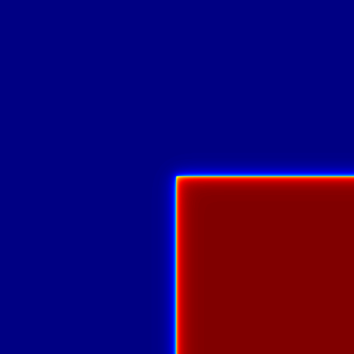
(n) CDF($T$=0.58)

Figure 16: Different images and their gradient CDFs (original image is from: beyondthehumaneye.blogspot.de).

Image set	1	2	3	4	5	6	7	all
$a_{1}$	8.62	7.88	7.76	8.34	9.13	8.07	8.89	8.37
$b_{1}$	0.51	0.52	0.54	0.52	0.54	0.53	0.55	0.53
$c_{1}\times 10^{5}$	-8.9	-5.0	-9.0	-4.3	-14	-5.6	-10	-6.3
SSE$\times 10^{-5}$	71	69	1.1	1.3	1.3	1.1	8.7	1.2
$R^{2}$	0.89	0.88	0.92	0.84	0.89	0.90	0.92	0.91
$a_{2}\times 10^{5}$	10.9	4.81	8.27	4.42	16.5	5.21	11.0	6.21
$b_{2}\times 10^{2}$	4.56	6.67	4.22	2.60	1.85	3.62	1.01	2.39
$c_{2}$	-4.74	-4.38	-4.60	-4.99	-5.79	-4.91	-6.03	-5.24
SSE$\times 10^{-5}$	1.13	0.892	1.32	1.47	1.72	1.26	1.17	1.48
$R^{2}$	0.83	0.85	0.90	0.82	0.86	0.89	0.89	0.90

Table 4: Parameters and goodness of fit of the two-dimensional models: Model 1 (top) and Model 2 (bottom).

As in the 1D case, we can use the model CDF alternatively to the PDF:

$$C(\vec{G})=\int\limits^{G^{y}}_{-\infty}\int\limits^{G^{x}}_{-\infty}P((u,v))\,\mathrm{d}u\mathrm{d}v\,.$$ (16)

We approximate the 2D joint CDF by the parametric model:

$$\widetilde{C}(\vec{G})=\widetilde{C}(G^{x})\widetilde{C}(G^{y})\,,$$ (17)

where $\widetilde{C}$ is defined in Eq. 12. The fitting results are shown in Table 5.

Image set	1	2	3	4	5	6	7	all
T	0.37	0.26	0.38	0.35	0.56	0.37	0.7	0.46
SSE	20.7	23.1	19.1	23.7	22.9	19.6	23.0	18.8
$R^{2}$	0.99	0.99	0.99	0.99	0.99	0.99	0.99	0.99

Table 5: Fits of the parametric 2D CDF model.

The 2D gradient CDF is sensitive to image transformations and potentially provides a powerful prior for the corresponding inverse problem. This is shown in Fig. 16, where an image is treated by different transformations and the corresponding CDFs are shown below. For the blurred image (Gaussian blur, $\sigma=3$), the frequency of small gradients is increased. For the noisy image ($10\%$ Gaussian noise), the frequency of large gradients is increased. For the super-resolution (SR) image (upsampling factor 9), the frequency of small gradients is increased. For the bilateral filter ($w=5$, $\sigma_{s}=3$, $\sigma_{c}=0.1$) and the guided filter ($r=10$, $\epsilon=0.01$), the frequency of small gradients is increased.

The model in Eq. 17 has only a single scalar parameter: $T$. This parameter can easily be determined by solving the following convex minimization problem:

$$\min_{T}\int(\log(p)+T^{2}(G^{x})^{2}+2\log(|G^{x}|))^{2}\mathrm{d}G^{x},$$ (18)

which has the unique analytical solution:

$$T=\left(\frac{-\int(2\log(|G^{x}|)+\log(p))(G^{x})^{2}\mathrm{d}{G^{x}}}{\int(G^{x})^{4}\mathrm{d}G^{x}}\right)^{\frac{1}{2}}.$$ (19)

Therefore, the parameter $T$ can directly be computed. The parameter $T$ leads to a linear gradient field remapping and guarantees an integrable gradient field. There is also an explicit relationship between parameter $a_{2}$ of the 1D marginal Model 2, and parameter $T$ of the 2D CFD model: $a_{2}=T^{2}$. This explains the good sensitivity of 1D Model 2 with respect to this parameter (see Fig. 13), and inspires the use of this parameter to define an image quality metric, as done next.

6.3 The Naturalness Factor

Comparing any image’s parameter $T$ with the expected value $T_{\text{pr}}$ from natural-scene images, i.e. from the GDP, we define:

Definition: For any image $I$, the naturalness factor $N_{\!f}$ is defined as $N_{\!f}=\frac{T}{T_{\text{pr}}}$ and the image $I_{n}$ generated from $I$ such that $T_{n}\approx T_{\text{pr}}$ is called the naturalized image.

Since $T_{\text{pr}}$ is obtained from the average gradient distribution of natural-scene images, the $N_{f}$ for a natural-scene image is expected to be one, as confirmed in Fig. 17. The range of possible values is $N_{f}\in[0.2,2.7]$, and the naturalness factor of natural-scene images satisfies a Log-Normally distribution (Fig. 17).

Figure 17: Naturalness Factor ($N_{f}$) distribution for the natural-scene images of the training set. Blue bars indicate $N_{f}<1$, red bars $N_{f}>1$. The black line is a Log-Normal distribution with parameters $\mu=0.039$ and $\sigma=0.613$.

6.4 Convexity, Sparsity, and Entropy of the GDP

The TV (Laplacian) prior is so popular because it leads to convex variational models. Even though the Hyper-Laplacian fits the data better, it leads to a non-convex model, which is harder to solve. We show here that our Model 2 (Eq. 11) and its 2D variant (Eq. 15) are quasi-concave, which means that all iso-sets are convex, hence simplifying optimization.

Lemma 6.1.

Eq. 11 and Eq. 15 are quasi-concave.

Proof.

For Eq. 11, we have:

$$\log(P(G_{1}^{x}))<\log(P(G_{2}^{x}))~{}~{}\mathrm{when}~{}~{}G_{1}^{x}>G_{2}^{x}>0$$ (20)

$$\log(P(G_{1}^{x}))<\log(P(G_{2}^{x}))~{}~{}\mathrm{when}~{}~{}G_{1}^{x}<G_{2}^{x}<0.$$ (21)

This monotonicity property with respect to 0 ensures that Eq. 11 is quasi-concave. Eq. 15 is a rotation of Eq. 11 with respect to the $y$ axis. Therefore, the set $\left\{\vec{G}\,:\,\log(P(\vec{G}))\geq h\right\}$ is convex $\forall h$. ∎

The overall energy function with Model 2 used as a prior, however, is not quasi-concave, but can be written as the difference of two convex functions. Such optimization problems are known as D.C. problems (short for: different of convex), and efficient solvers are available for them. The present model hence leads to efficiently solvable variational problems while still fitting the data better than previous models. Table 6 qualitatively compares different models.

Model	convexity	accuracy	computation cost
Eq. 10	quasi	high	medium
Eq. 11	quasi	high	low
Hyper-Laplacian	quasi	medium	low
Laplacian	yes	low	low
Gaussian	yes	very low	low
Eq. 14	no	high	medium
Eq. 15	quasi	high	low
2D Hyper-Lap	no	medium	low
2D Laplacian	yes	low	low
2D Gaussian	yes	very low	low
Eq. 17	no	medium	low

Table 6: Comparison of different models.

The gradient distribution balances sparsity and signal encoding. We define the sparsity of $p(\vec{G})$ as:

$$s_{p}(h)=\frac{\iint\chi_{p(\vec{G})>h}\mathrm{d}G^{x}\mathrm{d}G^{y}}{\iint\mathrm{d}G^{x}\mathrm{d}G^{y}},$$ (22)

where $\chi:R\rightarrow\{0,1\}$ is an indicator function. We further define:

$$C_{h}(h)=\iint\chi_{p(\vec{G})>h}p(\vec{G})\,\mathrm{d}G^{x}\mathrm{d}G^{y}\,,$$ (23)

which is the total probability mass on levels larger than $h$. The sparsity $s_{p}(h)$ measures how many words (of some dictionary) are needed to encode the information in $C_{h}(h)$ with an accuracy or tolerance $h$. The relationship between $s_{p}$ and $C_{h}$ is shown in Fig. 18 for the image data from the training set. We observe that the gradient signal is sparse already at a low cutoff $h$. Figure 19 shows the sparsity information curves for different parametric models of the GDP. Our Models 1 and 2 are about as sparse as the data, whereas all other models are less sparse and hence thrown away more information. This suggests that GDP could also be potentially interesting for compressed sensing [Donoho, 2006].

Figure 18: Sparsity of the gradient distribution. $98.2\%$ of the information can be encoded with only $2.5\%$ of the dictionary at a cutoff level of $h=3.6\times 10^{-6}$.

Figure 19: Sparsity comparison for different models.

The information of a signal is closely related to its entropy, describing the macroscopic behavior of the system as discussed above. The entropy of a 2D gradient distribution is defined as:

$$E(p)=-\iint p(\vec{G})\log(p(\vec{G}))\,\mathrm{d}G^{x}\mathrm{d}G^{y}\,.$$ (24)

Since the entropy is entirely determined by the gradient distribution, imposing a gradient prior implies imposing an entropy prior. The entropy distribution of the natural-scene images from the training dataset is show in Fig. 20. It is normally distributed. The average entropy and the entropies of different parametric models are given in Table 7.

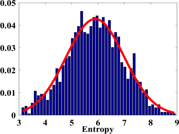
Figure 20: Entropy distribution of the natural-scene images from the training set. The average is 5.88. The red line is the Gaussian $0.043\exp\left[{-(\frac{E-5.89}{1.56})^{2}}\right]$.

	data	Eq. 14	Eq. 15	HyperLap	Laplace	Gaussian
Entropy	5.88	9.05	2.05	2.94	31.2	223

Table 7: Entropy of the training data and of different parametric models.

7 Correlation with Image Quality

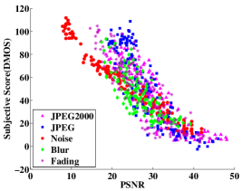
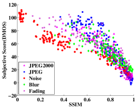
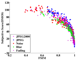
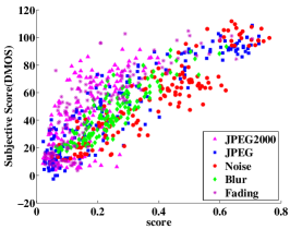
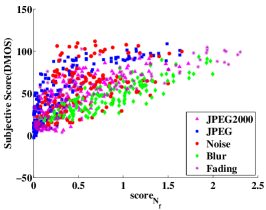
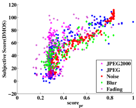
Figure 21: Image quality assessment results on the LIVE benchmark. We show the scatter plots of different objective image-quality measures (from left to right: PSNR, SSIM, FSIM; $score$, $score_{pr}$, $N_{\!f}$) with subjectively perceived image quality as quantified by the DMOS score. The different colors correspond to the different distortion in the LIVE benchmark, as given in the inset legends.

As a second key requirement for an image-processing prior, besides stability, we show next that the GDP is highly correlated with subjectively perceived image quality. We show that the distance between the gradient distribution of any given image and the GDP correlates with image quality. We use the standard LIVE benchmark dataset for image quality assessment [Wang et al., 2004]. In order to measure the distance between two gradient distributions, we test the $\ell_{2}$ norm, $\ell_{1}$ norm, cosine distance, the Earth Mover Distance (EMD), $\chi^{2}$ distance, and the Hellinger distance. Using this distance, we form the objective image-quality score:

$$score=Distance(p(\nabla I^{\mathrm{true}}),p(\nabla I^{\mathrm{distorted}})).$$ (25)

This can be further simplified to only use $N_{\!f}$:

$$score_{N_{\!f}}=|N_{\!f}^{\mathrm{true}}-N_{\!f}^{\mathrm{distorted}}|.$$ (26)

If the ground-truth image is unknown (i.e., in a real-world application rather than a benchmark setting), the score is defined with respect to the GDP:

$$score_{pr}=Distance(p^{\mathrm{pr}},p(\nabla I^{\mathrm{distorted}}))\,.$$ (27)

A measure of subjectively perceived image quality is provided by the LIVE benchmark’s DMOS (difference mean opinion score). Different correlations between DMOS and our objective score are reported in Tab. 8.

	$\ell_{2}$	$\ell_{1}$	cos	EMD	$\chi^{2}$	Hellinger
PCC	0.6193	0.7926	0.6277	0.5172	0.7662	0.8687
SCC	0.6434	0.7773	0.6114	0.7576	0.7977	0.8630
KCC	0.4588	0.5822	0.4355	0.5639	0.6027	0.6745

Table 8: Correlations between subjectively perceived image quality (DMOS from LIVE benchmark [Wang et al., 2004]) and our objective score using different distance metrics. The following correlations are reported: Pearson’s linear correlation coefficient (PCC), Spearman’s rank-order correlation coefficient (SCC), and Kendall’s rank-order correlation coefficient (KCC). In all cases, the Hellinger distance between the gradient distributions shows the best correlation.

In all cases, the Hellinger distance between the gradient distributions shows the best correlation. This suggests that using this distance metric, the GDP can directly be used to construct a novel image-quality measure. We compare this new measure (i.e., the score of Eq. 27) with other stat-of-art image quality assessment methods, such as PSNR (peak signal-to-noise ratio), SSIM [Wang et al., 2004], and FSIM [Zhang et al., 2011]. The results are shown in Fig. 21 and Table 9. The Hellinger distance between the gradient distribution of an image and the ground-truth GDP shows high linearity with DMOS, rendering the GDP a favorable prior for image processing. When used as an image-quality metric, however, the score without knowing ground truth ($score_{pr}$) is less good than specialized metrics like SSIM [Wang et al., 2004] and FSIM [Zhang et al., 2011] (Table 9). This is entirely expected, and it is not out aim to propose a new image-quality metric. However, since differences in the gradient distribution correlate with image quality, imposing the GDP is expected to improve an image’s quality. Together with its stability, this renders the GDP a good prior for practical applications, as illustrated in Sec. 9.

	PSNR	SSIM	FSIM	$score$	$score_{N_{f}}$	$score_{pr}$
PCC	-0.8585	-0.8252	-0.8586	0.8687	0.669	0.761
SCC	-0.8756	-0.9104	-0.9634	0.8630	0.712	0.706
KCC	-0.6865	-0.7311	-0.8337	0.6745	0.512	0.522

Table 9: Image quality assessment results on the LIVE benchmark.

8 Imposing the GDP in Variational Problems

In a variational framework, there are two ways to impose a prior: as a hard constraint or as a soft constraint. Both are possible for the GDP. For a hard constraint, the GDP is imposed by gradient remapping. The mapped gradient field is then used to reconstruct the output image by solving a Poisson equation with proper boundary conditions. For a soft constraint, the GDP can be imposed as a regularization term, leading to a minimization problem. As shown in Sec. 9, the decision between using a soft or hard constraint depends on the specific application.

8.1 As a hard constraint

We impose the GDP prior as a hard constraint by gradient-field remapping. The idea is to map the original gradient field, using a linear or nonlinear mapping function, into a new gradient field that exactly satisfies the prior. From this remapped gradient field, the output image is then reconstructed by solving a Poisson equation. In the special case of a linear mapping function, the reconstruction simplifies to rescaling the image pixel values.

While it is possible to directly map the input gradient field to the desired distribution [Coltuc et al., 2006b; Nikolova et al., 2013], such non-parametric mappings lead to numerical ambiguity due to discretization of the distribution into bins. This approach also does not guarantee the output gradient field to be integrable. We hence instead propose the use of parametric mapping functions. At the expense of some accuracy, they guarantee integrability of the result and lead to well-posed reconstruction problems.

8.1.1 Gradient field remapping

Let $Map$ remap the gradient field to a new field $\vec{G}_{n}$, which satisfies the GDP:

$$\vec{G}_{n}=Map(\vec{G}),\ \ s.t.\ \ p(\vec{G}_{n})=p^{\mathrm{pr}}.$$ (28)

In general, $Map$ can be non-parametric, parametric, nonlinear, or linear. A parametric nonlinear mapping leads to an integrable field, and the final image can be obtained by solving Poisson equation (Eq. 30), as outlined below. A linear parametric mapping leads to a simple rescaling of the pixel intensities and no Poisson equation needs to be solved. Fig. 22 illustrates the effects of different types of remapping. Linear remapping amounts to a simple rescaling of the intensities such that the gradient distribution fits the GDP in average. However, the fit obtained by nonlinear remapping is much better, but requires solving a Poisson equation. The gradient field entropies after remapping are 6.03 (original), 5.86 (reconstruction without remapping), 6.25 (linear remapping), and 5.79 (non-linear remapping), respectively. As expected, remapping makes the entropy of $\vec{G}_{n}$ closer to 5.88, the average entropy of natural-scene images.

8.1.2 Image reconstruction

Reconstructing the output image from the remapped gradient field amounts to minimizing the following $q\mbox{-}Dirichlet$ energy:

$$\begin{split}&\arg\min_{I_{n}}\left\{\|\nabla I_{n}-\vec{G}_{n}\|_{q}\right\}\\ &s.\,t.~{}~{}I_{n}\in Lip(\Omega)\,,\end{split}$$ (29)

where $q>1$, $\|\cdot\|_{q}$ is the standard $\ell_{q}$ norm, and $Lip(\Omega)$ is the space of Lipschitz-continuous functions on domain $\Omega$.

(a) Original

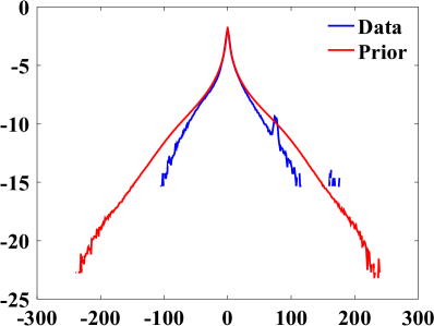
(b) Original

(c) Reconstruction w/o map

(d) Reconstruction w/o map

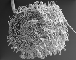
(e) Result with linear map

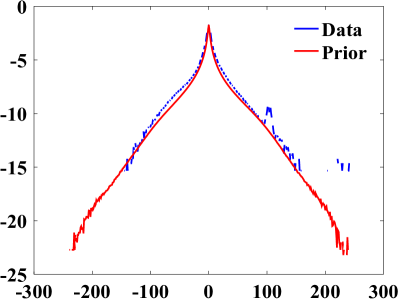
(f) Result with linear map

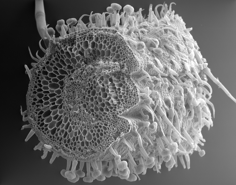
(g) Result with nonlinear map

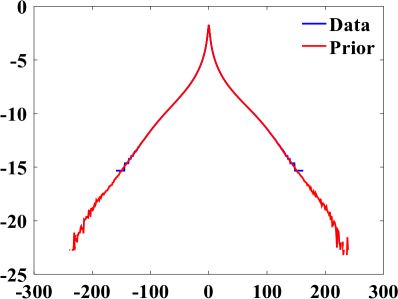
(h) Result with nonlinear map

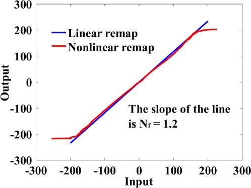
(i) Linear and nonlinear mapping functions used

Figure 22: Comparison of different gradient field remapping methods: original image and its gradient distribution (a,b), image reconstructed from original gradient field without any remapping (c,d), with linear remapping (e,f), and with nonlinear remapping (g,h) [Coltuc et al., 2006b]. The absolute RMS of the reconstructions are 0, 2.0, 23, and 33, respectively, with respect to the original image. The corresponding gradient distributions after remapping are shown to the right of the images. The linear and nonlinear remapping functions used are shown in (i).

Existence and uniqueness of the solution of Eq. 29 have been proven [Boccardo et al., 1996]. Commonly used norms are $\ell_{2}$ ($q=2$) and $\ell_{1}$ ($q=1$), which correspond to reducing measurement errors (unspecific) and gross errors (outliers), respectively.

Taking the $\ell_{2}$ norm in Eq. 29, we recover the output image $I_{n}$ from the remapped gradient field $\vec{G}_{n}$ by solving the Poisson equation:

$$\Delta I_{n}=\nabla\cdot\vec{G}_{n}\,.$$ (30)

This equation can be solved efficiently, e.g., by FFT-based algorithms or wavelet solvers. A short summary of available Poisson solvers is given in Table 10.

Reconstructing an image from its gradient field is accurate. An example is shown in Fig. 22(c). The original image (a) is an 8-bit grayscale image. The absolute RMS of the reconstruction without remapping (b) is 2.032 with an average intensity value of 104.9. The size of the image is $1881\times 2400$ pixels. Reconstruction using the wavelet solver in Matlab takes about 3.5 seconds on an Apple MacBook Pro (early 2011).

Solver	Cholesky	Jacobi	Gauss-Seidel	SOR
Type	direct	iterative	iterative	iterative
Complexity	$(mn)^{3}$	$(mn)^{2}$	$(mn)^{2}$	$(mn)^{3/2}$
Solver	Cholesky	FFT	Multigrid	Wavelet
Type	direct	direct	iterative	direct
Complexity	$(mn)^{3/2}$	$(mn)log(mn)$	$(mn)$	$(mn)$

Table 10: Summary of Poisson solvers. The FFT and Wavelet-based solvers are implemented in our software package.

8.2 As a soft constraint

Imposing the GDP as a soft constraint is done by using the GDP as a regularization term. For a variational function $\mathcal{E}(\hat{U})$ this can be done by evolving the PDE

$$\frac{\partial\hat{U}}{\partial t}=-\frac{\partial\mathcal{E}(\hat{U})}{\partial\hat{U}}$$ (31)

over pseudo-time $t$ (i.e., the iterations of the algorithm). Since the energy is $\mathcal{E}$ non-convex in general, minimization should be performed in a multi-scale space in order to avoid local minima and accelerate the computation. This can for example be done using multi-scale anisotropic diffusion, similar to the Perona-Malik model [Perona and Malik, 1990]. More details about this procedure are given in Sec. 9.3.

When using our parametric Model 2 for the GDP, the minimization problem further simplifies. In this case, the variational energy is the difference of two convex functions, and the minimization problem can efficiently be solved using algorithms based on D.C. programming [Hamdi, 2006]. Then, the following decomposition holds:

$$\mathcal{E}(U)=\mathcal{E}_{1}(U)-\mathcal{E}_{2}(U)\,,$$ (32)

where $\mathcal{E}_{1}(U)=\int_{\vec{x}\in\Omega}(\frac{1}{2}\|U-I\|_{*}+\frac{\lambda}{2}T_{\mathrm{pr}}^{2}\|\nabla U\|_{2}^{2})\mathrm{d}\vec{x}$ and $\mathcal{E}_{2}(U)=-\frac{\lambda}{2}\int_{\vec{x}\in\Omega}\log(b_{\mathrm{pr}}+\|\nabla U\|_{2}^{2})\mathrm{d}\vec{x}$ are differentiable convex functions, and $b_{\mathrm{pr}}$ is the GDP value of parameter $b_{2}$ of Model 2.

One way to solve such problems is to use Bregman splitting techniques [Hamdi, 2006]. In this case, one needs to choose a Bregman function $\phi$, the choice of which however does not matter much to the algorithm performance [Hamdi, 2006]. Then, Eq. 32 can be minimized using Algorithm 1. The convergence proof can be found in [Hamdi, 2006; Gasso et al., 2009]. In the special case when $\phi$ is chosen to be a quadratic function, Algorithm 1 reduces to the standard proximal point algorithm.

Algorithm 1 Minimization using D.C. programming

0:  $\mathcal{E}_{1}$, $\mathcal{E}_{2}$, $\phi$, step size $\delta t>0$, $\epsilon>0$

1:  while $\|(U_{i}-U_{i-1})\|_{\infty}>\epsilon$ do

2:     $U_{i+1}=(\nabla\phi+\delta t\nabla\mathcal{E}_{1})^{-1}(\nabla\phi(U_{i})+\delta t\nabla\mathcal{E}_{2}(U_{i}))$

3:  end while

8.3 Implementation details

For hard GDP constraints, we implemented nonparametric remapping based on exact histogram specification [Coltuc et al., 2006a] and remapping based on our parametric Model 2. For image reconstruction, we implemented FFT(DST, DCT)-based and wavelet-based Poisson solvers.

For soft GDP constraints, we implemented the multi-scale diffusion (Perona-Malik model [Perona and Malik, 1990]), which is valid for all priors. Specifically for our Model 2, we also implemented the D.C. programming of Algorithm 1.

The source code is available from our website as Matlab code, C++ code included in the OpenCV library, and Java code as an ImageJ/Fiji plugin.

9 Example Applications

Priors play a central role in many image processing tasks. We exemplify this here by showing the use of the present GDP, the parametric models, and the solvers in a wide variety of image-processing tasks, ranging from contrast enhancement, to noise level estimation, denoising, deconvolution, zooming (super resolution), and dehazing.

9.1 Image naturalization

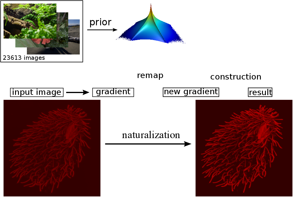
Figure 23: Naturalization.

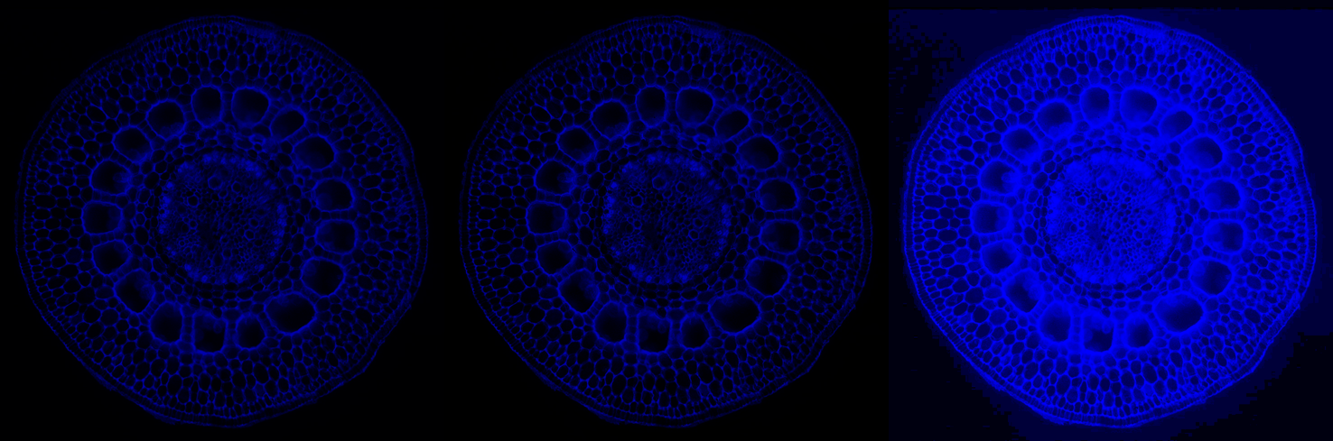
(a) $N_{\!f}=1.07$ (beyondthehumaneye.blogspot.de)

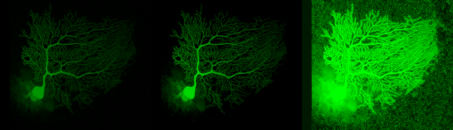
(b) $N_{\!f}=1.51$ (Maryann Martone, CCDB)

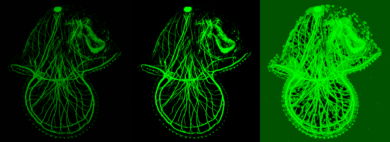
(c) $N_{\!f}=1.81$ (Lee & Matus, U Hawaii, amicros.org)

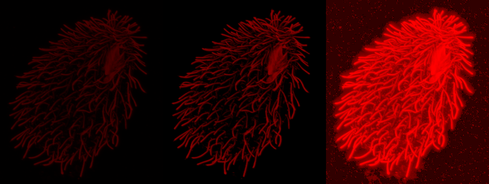
(d) $N_{\!f}=2.00$ (Gaertig lab, U Georgia, bmc.uga.edu)

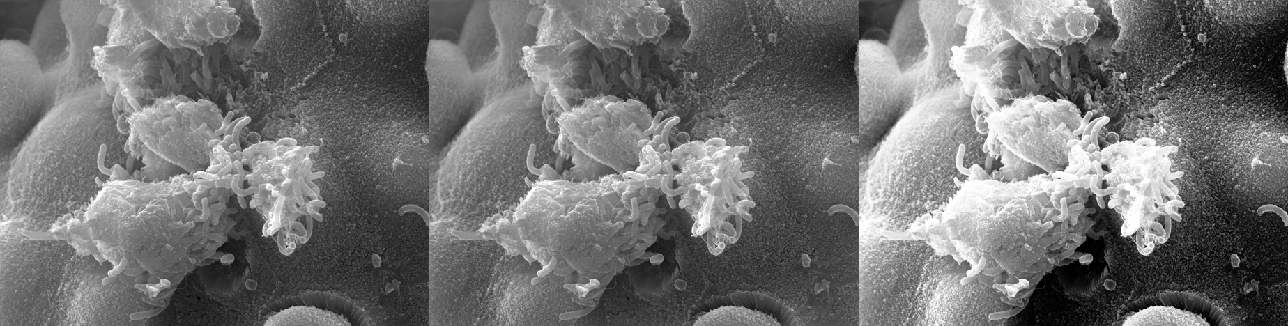
(e) $N_{f}=1.03$ (Dartmouth EM Gallery)

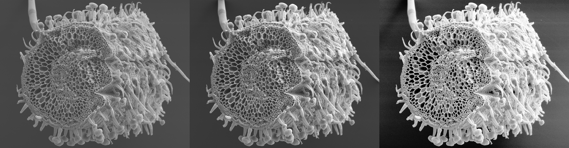
(f) $N_{\!f}=1.27$ (Dartmouth EM Gallery)

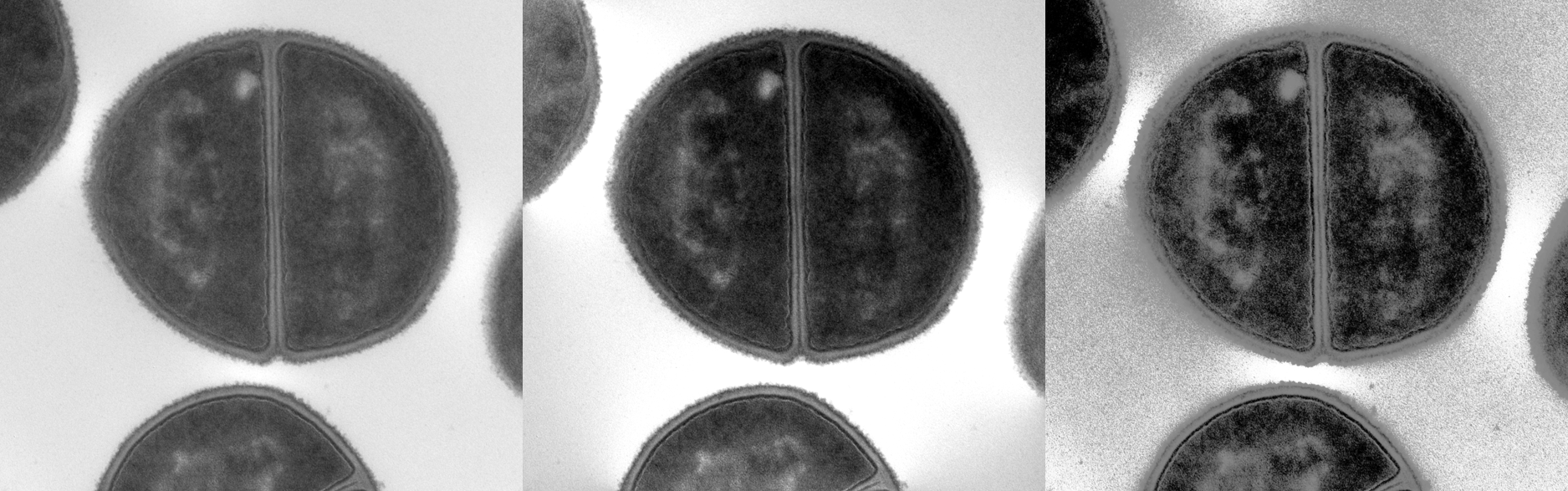
(g) $N_{\!f}=1.45$ (Dartmouth EM Gallery)

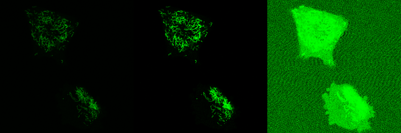
(h) $N_{\!f}=2.29$ (K. Ushakov, U Geneva)

Figure 24: Examples of original (left), naturalized (middle) and histogram equalized (right) microscopy images.

Remapping the gradient field of any image to match the GDP of natural-scene images, and then reconstructing the output image is called image naturalization, because the output image will have a gradient distribution that matches the one of natural-scene images. The naturalized output image hence looks more “natural”. The workflow is shown in Fig. 23. Since the GDP correlates with image quality, this makes the image look more appealing. We hence propose to use image naturalization as an alternative to histogram equalization when displaying images to a human observer. Image naturalization enhances contrast by solving Eq. 2 with hard GDP constraint. Some examples of microscopy images (left tile of each panel) and their naturalized versions (middle tiles) are shown in Fig. 24 along with the naturalness factor of the original image. The histogram-equalized images are shown in right tiles for comparison. The first row shows four fluorescence-microscopy images. The second row shows three electron-microscopy images and one fluorescence image. All images were collected from publicly accessible web pages; credits are in parentheses. Here we use the simple linear $Map$ function, amounting to a straightforward rescaling of the image, albeit with a good, “natural” scale factor as determined by the GDP. In all cases. the naturalized image looks more appealing than the histogram-equalized image, and suffers from less background artifacts.

9.2 Noise level estimation

Traditional denoising methods heavily rely on having an estimate of the noise level to adjust their parameters. In practical applications, however, the true noise level is unknown. We show how the GDP can be used to robustly estimate the noise level of an image. As shown by the noise case in Fig. 16, the parameter $T$ of Model 2 is sensitive to noise. This can be exploited to estimate the noise level by relating the fitted parameter $T$ of any given image to noise level through a calibration curve. We construct such a calibration curve ($T$ vs. true noise level) by randomly choosing seven images from our natural-scene training dataset and adding to them Gaussian noise of varying $\sigma=[0.02:0.02:0.8]$. The dependence of $T$ on $\sigma$ shows a distinct characteristic, which is almost independent of image content (left panel of Fig. 25, 7 curves with different symbols). We fit this dependence using the mixture of exponentials:

$$\widetilde{\sigma}=\sum_{i=0}^{i=N}q_{i}\exp\!{\left\{s_{i}T\right\}},$$ (33)

where $q_{i}>0$ and $s_{i}<0$ are parameters to be determined. For our dataset, we find the best fit $N=2$, $q_{\{1,2\}}=\{772.6,0.9538\}$, $s_{\{1,2\}}=\{-5321,-931.2\}$. The goodness of fit is: SSE=0.2741, RMSE=0.034, $R^{2}$=0.979. The model is shown by the solid blue line in the left panel of Fig. 25.

We test the model by adding Gaussian noise of different, known $\sigma$ to a disjoint randomly selected set of seven image (the test set for cross validation). The differences between the noise levels $\widetilde{\sigma}$ estimated by our model and the ground truth are shown in the right panel of Fig. 25. 87% of the predictions have an accuracy $|\widetilde{\sigma}-\sigma|<0.04$. We find similar results also for other random image sets tested.

This suggests that the parameter $T$ can provide accurate and robust noise-level estimation. A particularly favorable property of this estimator is its high sensitivity to changes in $\sigma$ for low noise levels ($\sigma<0.2$). Correctly estimating low noise levels is particularly hard for traditional, pixel-based estimators.

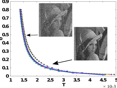
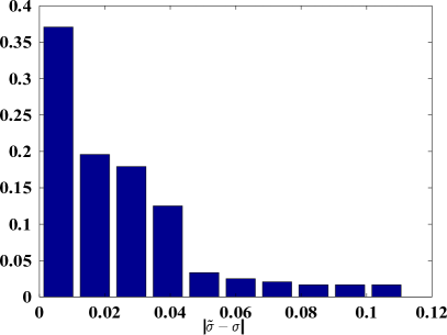
Figure 25: Noise-level model and its prediction-error distribution.

9.3 Denoising

The high sensitivity of the cumulative gradient distribution to small levels of noise makes the GDP a good prior for image denoising. Small non-zero gradients play a key role to recover image details. Traditional denoising methods with spatial regularization (such as TV and its variants, GC, etc.) remove both noise and small signal gradients. In contrast, the GDP can be used to distinguish between noise and small signal gradients. This is compatible with many researchers’ observation that split-Bregman solvers for TV-$\ell_{1}$ models achieve better results in the sense of PSNR [Goldstein and Osher, 2009; Paul et al., 2013]. This is because the auxiliary variable introduced in Bregman splitting changes the model to allow small gradients. These small gradients improve the result. Another example is non-local TV, using spatially repeated patterns to allow for small signal gradients [Liu and Huang, 2014]. A third example is stochastic (Monte Carlo) denoising [Wong et al., 2011]. While all of these methods allow for small image gradients, distinguishing them from noise is mostly ad hoc and arbitrary. Here, the GDP can provide additional information. This has recently been demonstrated in a MAP Bayesian framework [Cho et al., 2012], which also has the capability of recovering image details. Using our novel parametric GDP model, we introduce:

$$\begin{split}\mathcal{E}(U)=&\int_{\vec{x}\in\Omega}\frac{1}{2}\|U-I\|_{2}^{2}+\\ &\frac{\lambda}{2}(T_{\mathrm{pr}}^{2}\|\nabla U\|_{2}^{2}+\log(b_{\mathrm{pr}}+\|\nabla U\|_{2}^{2}))\mathrm{d}\vec{x}.\end{split}$$ (34)

This denoising model is differentiable with respect to $U$ and can be efficiently solved by gradient descent (Algorithm 2). Using the Gâteaux derivative, this model can be interpreted as an anisotropic diffusion and inverse diffusion process:

$$\begin{split}\frac{\partial U}{\partial t}&=-\frac{\partial\mathcal{E}}{\partial U}\\ &=I-U+\lambda\left(T^{2}_{\mathrm{pr}}+\frac{b_{\mathrm{pr}}-\|\nabla U\|_{2}^{2}}{(b_{\mathrm{pr}}+\|\nabla U\|_{2}^{2})^{2}}\right)\Delta U.\end{split}$$ (35)

This equation can also be derived from the Euler-Lagrange equation of the variational form.

The regularization term is a hybrid of diffusion and inverse diffusion, which is fundamentally different from traditional approaches that only depend on one of them. For example, the traditional anisotropic diffusion $(1+\|\nabla U\|_{2}^{2})^{-1}$ (Perona Malik model [Perona and Malik, 1990]) only tries to smooth the image, while inverse diffusion only enhances the image [Calder and Mansouri, 2011]. The behavior of the diffusion coefficient $W$ in Algorithm 2 is illustrated in Fig. 26. It is clear that $U$ gets enhanced (inverse diffusion, $W<0$) or smoothed (diffusion, $W>0$) depending on the gradient magnitude. Even though this behavior is similar to forward-backward diffusion [Gilboa et al., 2002], the fundamental difference is that our model is derived from a distribution prior, rather than from the gradient itself. As a result, the parameters $T_{\mathrm{pr}}$ and $b_{\mathrm{pr}}$ are learned from datasets and do not need to be manually adjusted, as in forward-backward diffusion [Gilboa et al., 2002].

An example of using this model for denoising as given in Algorithm 2 is shown in Fig. 27 and Table 11. The present model achieves state-of-the-art PSNR with significantly better image quality, quantified by the SSIM quality measure in Table 11.

0:  $I$, $\lambda$, step size $\delta t$, $T_{\mathrm{pr}}$, $b_{\mathrm{pr}}$, $\epsilon$

1:  while $\|(U_{i}-U_{i-1})\|_{\infty}>\epsilon$ do

2:     $W=T_{\text{pr}}^{2}+\frac{b_{\mathrm{pr}}-\|\nabla U\|_{2}^{2}}{(b_{\mathrm{pr}}+\|\nabla U\|_{2}^{2})^{2}}$

3:     $U_{i+1}=\frac{U_{i}}{1+\delta t}+\frac{\delta t}{1+\delta t}I+\frac{\delta t}{1+\delta t}\lambda W\Delta U_{i}$

4:  end while

Algorithm 2 Denoising with GDP

Lemma 9.2.

In Algorithm 2, let $v=\|\nabla U\|_{2}^{2}$, if $T^{2}_{\mathrm{pr}}b_{\mathrm{pr}}\geq\frac{1}{8}$, then $W\geq 0$. If  $T^{2}_{\mathrm{pr}}b_{\mathrm{pr}}<\frac{1}{8}$, then there are two fixed points $v_{L}$ and $v_{U}$ ($v_{L}<v_{U}$) such that

$$\begin{cases}W\leq 0&if~{}~{}v_{L}\leq v\leq v_{U}\\ W>0&else.\\ \end{cases}$$ (36)

This is illustrated in Fig. 26. The proof is given in Appendix A.

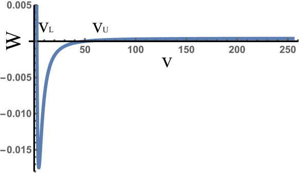
Figure 26: Behavior of the diffusion coefficient $W$ versus the square gradient magnitude $v=\|\nabla U\|_{2}^{2}$ for the $T^{2}_{\mathrm{pr}}$ and $b_{\mathrm{pr}}$ values of the GDP.

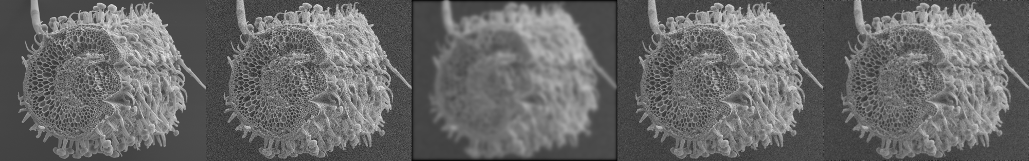
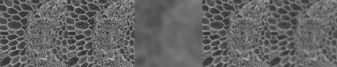
Figure 27: Denoising example. From left to right: original image, noisy image, solution of the Perona-Malik model [Perona and Malik, 1990], solution of the TV model, solution of our GDP model. A magnified patch is shown under each image.

	noisy	Perona-Malik	TV	Present
PSNR	17.12	20.72	26.39	26.39
SSIM	0.2087	0.5534	0.6441	0.7196

Table 11: Quality comparison of denoising results from different models.

9.4 Blind Deconvolution

Biomedical images are often blurred, e.g., due to object motion during exposure, or due to light diffraction in the detector optics. The latter is particularly common in microscopy, where the imaged objects are of similar length scale as the wavelength of the light used. The image is then significantly blurred by the point-spread function (PSF, or impulse-response function) of the optics, the Fourier transform of which is the optical transfer function of the imaging equipment. Since this blurring is an artifact of the imaging method, one often seeks to undo it to the extent possible. In fluorescence microscopy, the imaging process is linear, and the blurring is accurately described by a convolution of the original image with the PSF of the microscope. The task of deconvolution is to estimate the perfect latent image $U$ from the observed blurred image $I$. If the PSF (blur kernel) $K$ is unknown and to be estimated along, the problem is referred to as blind deconvolution. This is a typical ill-posed inverse problem. Imposing a prior can render the problem well posed.

$K$ and $U$ can be estimated either in the spatial and/or the gradient domain. We provide here an algorithm for blind deconvolution using GDP. The algorithm is inspired by Fig. 4, showing that auto-correlation is significantly reduced in the gradient domain, which is a favorable property for (blur-)kernel estimation. The latent image, however, is better estimated in the spatial domain, where the auto-correlation signal can be exploited. Different combinations of spatial/gradient-domain deconvolution have already been priorly presented (see Table 12). The present algorithm, however, is the first one to combine gradient-domain kernel estimation with spatial-domain image estimation, which we believe to be a particularly good combination.

	Kernel $K$	Image $U$	Typical Method
domain	spatial	spatial	[Levin et al., 2007]
	spatial	gradient	[Fergus et al., 2006]
	gradient	gradient	[Chen et al., 2010]
	gradient	spatial	present

Table 12: Summary of blind deconvolution algorithms.

Besides the working domain, the prior (or regularizer) used is of key importance. In general, sparsity of the kernel and TV of the latent image are imposed for deconvolution [Chan and Wong, 1998; Marquina, 2009; Krishnan et al., 2011; Li et al., 2012]. However, it is known that a GDP on the latent image provides a better choice, removing less image detail than TV [Fergus et al., 2006; Krishnan and Fergus, 2009; Cho and Lee, 2009; Chen et al., 2010; Shan et al., 2008]. Here, we use the present parametric GDP model as a prior for the latent image, but impose no prior on the kernel. This renders our methods generic to a wide variety of different blur kernels that do not have to be priorly known.

We use alternating minimization to estimate the kernel $K$ and the latent image $U$ by minimizing:

$$\begin{split}\mathcal{E}_{k}(K)&=\|\nabla U_{i}\otimes K-\nabla I\|_{2}^{2}\ \\ &s.t.~{}~{}\|K\|_{2}=1\,,K\geq 0\,.\end{split}$$ (37)

$$\begin{split}&\mathcal{E}_{u}(U)=\frac{1}{2}\|U\otimes K_{i+1}-I\|_{2}^{2}\\ &+\frac{\lambda}{2}\left(T_{\mathrm{pr}}^{2}\|\nabla U\|_{2}^{2}+\log(b_{\mathrm{pr}}+\|\nabla U\|_{2}^{2})\right)\,,\end{split}$$ (38)

where $i$ is the iteration number of the alternating minimization scheme. Equation 37 is a convex function with convex constraints, guaranteeing a globally optimal solution. In Algorithm 3 we hence solve this part of the problem analytically by projection. Equation 38 is not convex, but can be solved by a diffusion process. Algorithm 3 summaries the resulting overall blind deconvolution process, which is performed in a multi-scale fashion to avoid local minima and accelerate computation. A notable implementation detail is that we only compute on the interior pixels in order to avoid the boundary issue, instead of padding the image as done in previous methods.

An example with a complicated blur kernel is shown in Fig. 28 and Table 13. The ground-truth image (Fig. 28(a)) is blurred with a known kernel (Fig. 28(b)). Figure 28(c,d) show the reconstructed images using two different non-blind deconvolution methods with the ground-truth kernel provided to them. Figure 28(e,f) show the results of two blind deconvolution methods along with the estimated kernels (insets). Figure 28(g) shows the estimated $\hat{K}$ at different scales of the multi-scale process used in the present method. As evident from Table 13, the result from the present GDP method achieves higher image quality (as measured by SSIM) than the comparison algorithms.

Algorithm 3 Blind Deconvolution with GDP

0:  $I$, $\lambda$, $T_{\mathrm{pr}}$, $b_{\mathrm{pr}}$,$\epsilon$

1:  ${\bf F}_{I}=FFT(\nabla I)$

2:  while $\|\nabla(U_{i}-U_{i-1})\|>\epsilon$ do

3:     ${\bf F}_{U}=FFT(\nabla U_{i})$

4:     $\hat{K}_{i+1}=FFT^{-1}\left(\frac{\overline{{\bf F}_{U}}^{T}\circ{\bf F}_{I}}{\overline{{\bf F}_{U}}^{T}\circ{\bf F}_{U}}\right)$

5:     $K_{i+1}\leftarrow\hat{K}_{i+1}>0,\int_{\vec{x}\in W_{K}}\hat{K}_{i+1}\mathrm{d}\vec{x}=1$

6:     $U_{i+1}\leftarrow$ Anisotropic Diffusion $U_{i}$ with $K_{i+1}$ (Eq. 35)

7:  end while

(a) ground truth image

(b) blurred image with $K$

(c) Lucy-Richardson result

(d) Hyper Laplace Prior result

(e) normalized sparsity result

(f) present GDP result

(g) estimated $\hat{K}$ at different scales of our method

Figure 28: Image deconvolution example. (a) Ground truth image. (b) Input image to the deconvolution methods, obtained by blurring the image in (a) with the kernel shown in the inset. (c,d) Results from two non-blind deconvolution methods with the ground truth blur kernel given; the classical Lucy-Richardson algorithm [Biggs and Andrews, 1997] and the hyper-Laplace method [Krishnan and Fergus, 2009]. (e,f) Results from two blind deconvolution methods ([Krishnan et al., 2011] and our GDP) along with the estimated blur kernels (insets). (g) Blur kernel estimated by our method on different levels of the multi-scale process.

	PSRN	SSIM
Blurred input image (Fig. 28(b))	23.85	0.58
Lucy-Richardson (Fig. 28(c))	27.44	0.72
Hyper-Laplacian (Fig. 28(d))	23.87	0.68
Normalized sparsity (Fig. 28(e))	27.34	0.73
Present method (Fig. 28(f))	33.69	0.92

Table 13: Quality comparison of deconvolution results.

A recent development in deconvolution is to use image patches instead of the whole image to accelerate kernel estimation [Hu and Yang, 2012; Bae et al., 2012]. This can easily be adopted also in our framework, provided the patches are large enough for the GDP to be valid within them (see Section 10).

9.5 Zooming and Super Resolution

Zooming or super-resolution (SR) is the process of resampling an image (or a part of an image) onto a larger grid of pixels. Increasing the number of pixels in the image while keeping the field of view the same hence increases the image resolution. The interesting question is then how to interpolate the image information onto the finer pixel grid where no information is available on the course input grid. We show here how the same algorithm as for deconvolution can also be used for zooming. The only change is that we use an up-sampled $U$ (i.e., $U$ has more pixels than $I$) and a known Gaussian kernel $K(\vec{x})=\frac{1}{\sqrt{2\pi}\sigma}e^{-\|\vec{x}\|^{2}/\sigma^{2}}$ in Eq. 38. We do not need to iterate Eq. 37, because the kernel is known in this application. An example is shown in Fig. 29. For fun, we compare the resulting zoomed image with an image of the same sample acquired by a true super-resolution microscopy technique (here: PALM microscopy). While zooming with the present algorithm renders the image crisper (due to the deconvolution kernel) and better resolved (due to the finer pixel grid), it does not actually improve the optical resolution of the microscope. This can nicely be observed when two filaments cross. In the zoomed image there is a gap at the crossing point, whereas the PALM microscopy image properly resolves both filaments crossing.

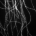
(a) original $128\times 128$

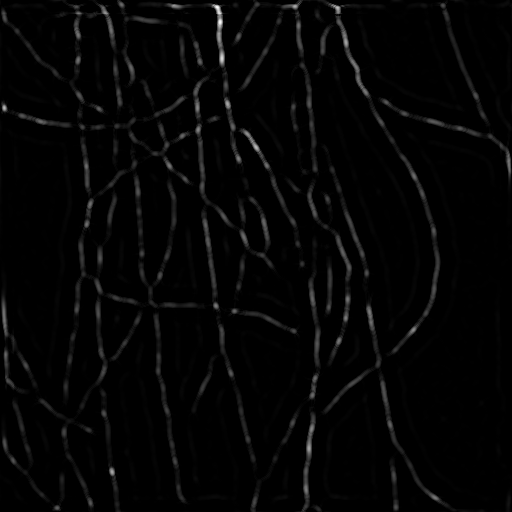
(b) zoomed $512\times 512$

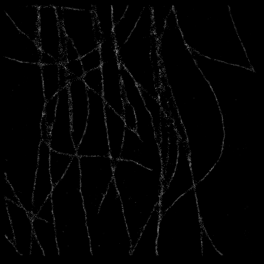
(c) PALM $512\times 512$

Figure 29: Zooming using the GDP. Panel (b) shows the zoomed version (up-sampling factor 4) of the fluorescently labeled microtubules in (a) as computed using the present method. Panel (c) shows a real super-resolution PALM image of the same scene for comparison. ((a)&(c) from: EPFL Collection of Reference Datasets, bigwww.epfl.ch/smlm/datasets/index.html?p=real-hd)

9.6 Scatter Light Removal and Dehazing

Scatter light is a common nuisance in light microscopy when imaging thick samples. The light propagating though the sample is scattered (Rayleigh and Mie scattering), similarly to how fog or haze scatters light in a natural-scene photograph. The resulting image is the superposition of the scatter light and the latent image. In classical dehazing methods, the observed image $I$ is modeled as [He et al., 2011]:

$$I(\vec{x})=U(\vec{x})t(\vec{x})+A(1-t(\vec{x}))\,,$$ (39)

where $U$ is the latent image, $t(\vec{x})=e^{-\beta d(\vec{x})}$ is the unknown transmission map, and $A$ is the environment light constant. The unknown parameter $\beta$ is a material constant (scattering coefficient), and $d(\vec{x})$ is the distance from the scene to the camera. Solving this model for $U$ is ill-posed. A popular prior to regularize the problem in the spatial domain is the dark-channel prior [He et al., 2011]. Alternatively, the problem can be regularized in a Bayesian framework [Nishino et al., 2012]. Here, we impose the GDP for the latent image and TV for the transmission map as hard constraints:

$$\begin{split}\mathcal{E}(U,t)=&\frac{1}{2}\left\|U(\vec{x})t(\vec{x})+A(1-t(\vec{x}))-I(\vec{x})\right\|_{2}^{2}\\ &s.t.~{}~{}p(U(\vec{x}))=p^{\mathrm{pr}},~{}p(t(\vec{x}))=p^{\mathrm{pr}}.\end{split}$$ (40)

Unlike previous works, Eq. 39 does not hold anymore in our model. Instead, our model can be written as:

$$\begin{split}&\mathcal{E}(U,t)=\frac{1}{2}\left\|U(\vec{x})t(\vec{x})+A(1-t(\vec{x}))-I(\vec{x})\right\|_{2}^{2}+\frac{\lambda}{2}\\ &\left[T^{2}\|\nabla U(\vec{x})\|_{2}^{2}+\log(b+\|\nabla U(\vec{x})\|^{2}_{2})+\alpha\left\|\frac{\nabla t(\vec{x})}{t(\vec{x})}\right\|_{1}\right].\end{split}$$ (41)

We use alternating minimization over $U$ and $t$ to obtain the final result. An example is shown in Fig. 30. Using simple Otsu thresholding on the original image does not allow detecting any objects in the image. Instead, they are fused to one large blob by the scatter light. After dehazing using the present method, the same simple Otsu thresholding allows object segmentation.

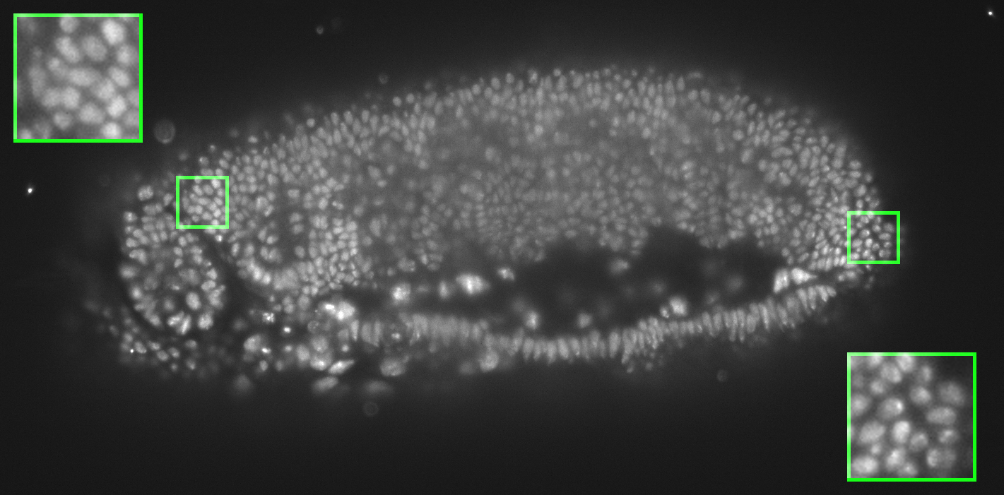
(a) Original

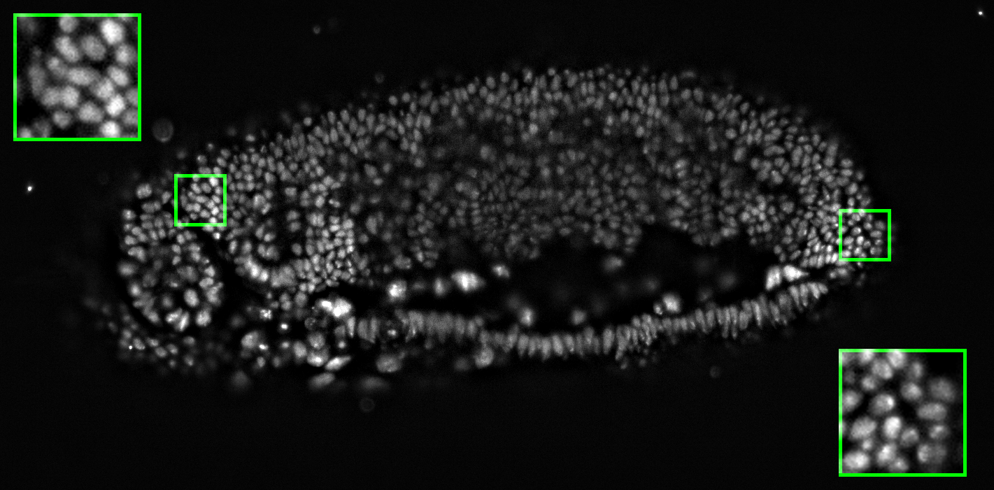
(b) Present dehazing result

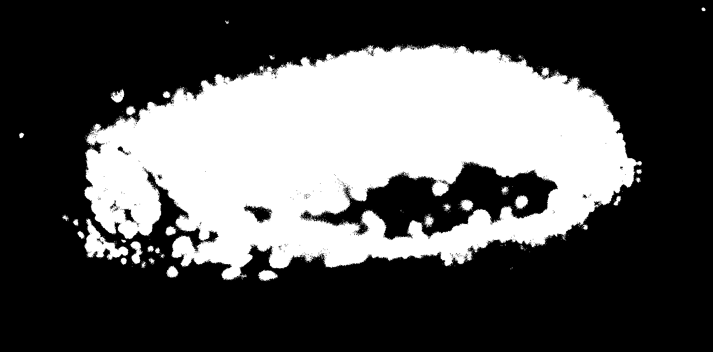
(c) Otsu thresholding of (a)

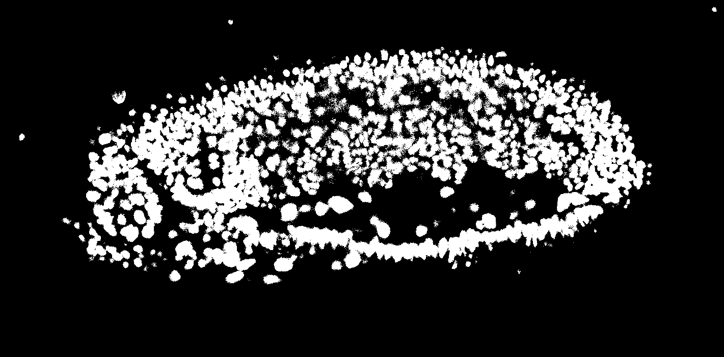
(d) Otsu thresholding of (b)

Figure 30: Scattering light removal in a SPIM microscopy image of a whole Drosophila embryo with the Nuclei labeled by fluorescence. (a) Original image as recorded by SPIM microscopy (source: Tomancak lab, MPI-CBG). Due to the thickness of the sample, there is significant scatter light, prohibiting object segmentation using thresholding (c). (b) Result from the present dehazing method, enabling object thresholding (d). Insets show zoomed details as indicated by the green boxes.

9.7 The Naturalness Factor as an Image Feature

The naturalness factor $N_{\!f}$ is a scalar number that is easy to compute. It can hence provide an interesting image feature, for example in classification or machine-learning frameworks when the naturalness of an image is to be quantified. We illustrate this by classifying transmitted light microscopy images of marine phytoplankton from natural-scene images. We collected a dataset of 1322 images of 45 different species of phytoplankton. Some example images are shown in Fig. 31(a). Figure 31(b) shows the histogram of $N_{\!f}$ of all images. Despite the fact that the images look visually diverse, they mostly have similar $N_{\!f}$, which moreover is clearly different from that of natural-scene images (see Fig. 17). The naturalness factor could hence be used as an important feature to classify these images.

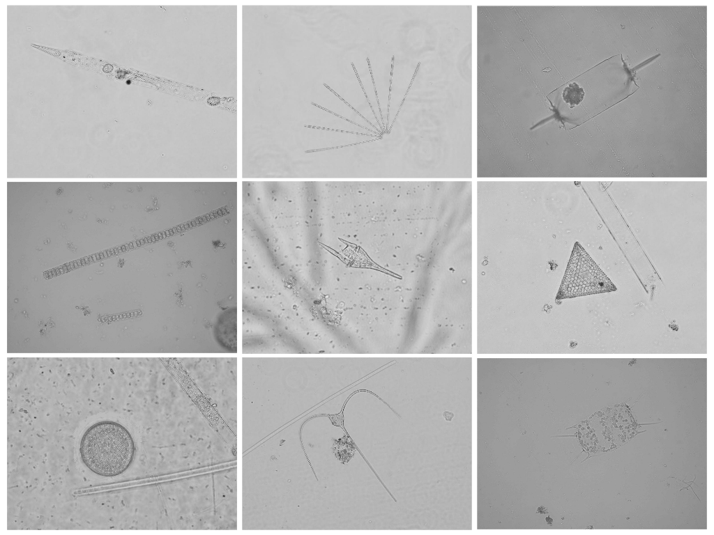
(a) sample images

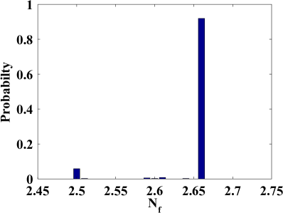
(b) $N_{\!f}$ histogram

Figure 31: $N_{\!f}$ distribution of light-microscopy images of marine phytoplankton. Even though the images show plankton of very different morphologies, their $N_{\!f}$ is mostly the same, hence providing a classification feature for these images.

10 Conclusion and Discussion

We proposed learning a gradient distribution prior (GDP) for biomedical images from natural-scene images. We provided different lines of argument why we believe this is worthwhile doing, and we have established that the resulting prior is stable and correlated with image quality. We have provided novel parametric models for GDP. Our models are of different accuracy and complexity, some of them leading to very simple convex problems. We have illustrated this in various applications, ranging from image enhancement to denoising, deconvolution, and dehazing. In all cases, the present GDP models led to results that were comparable or better than the existing state of the art in the respective field of application. We have further established a relationship between our GDP, traditional TV regularization, and anisotropic diffusion.

While we have exclusively focused on the image gradient here, the same work could also be done for higher-order derivatives, like the Laplacian. Spectral statistics of higher-order differential operators could provide additional regularization in the same framework. Of special interest could also be the mean or Gaussian curvature (GC) distributions Gong and Sbalzarini [2013], as it directly relates to the geometry of cell membrane through the Willmore energy. As shown in Fig. 32, all of these second-order derivatives satisfy similar distributions as the gradient. Using GC as a prior is well known to better preserve edges in the image than mean curvature or the Laplacian. Figure 32, however, suggests the opposite. This needs more research. An interesting observation is that the naturalness factor derived from the distribution of the Laplacian is highly correlated with that derived from the gradient distribution (Fig. 33). This suggests that the naturalness factor is a universal image feature that does not depend on the order of the statistic over which it is defined. Confirming this, however, is still outstanding.

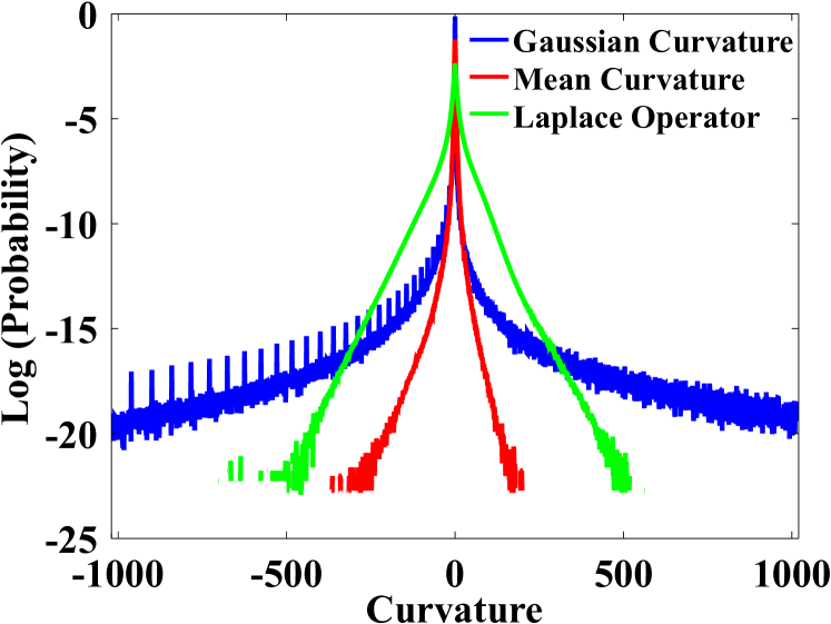
Figure 32: Average distribution of Gaussian curvature, mean curvature, and Laplace operator response across all training images of our natural-scene image dataset.

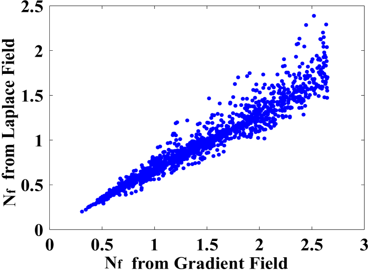
Figure 33: the naturalness factors computed from the gradient and the Laplacian distributions are highly correlated.

The present work can also be extended to higher-dimensional images. Constructing and using, for example, a GDP for 3D biomedical images is straightforward. The parametric models presented here are simple sums or products of 1D models and can hence trivially be extended to higher dimensions. As an example, Fig. 34 shows the predicted gradient distribution in 3D using our Model 1. However, it is not easy to verify this result, because there are (almost) no 3D natural-scene images, and 3D biomedical images are corrupted by noise and blur.

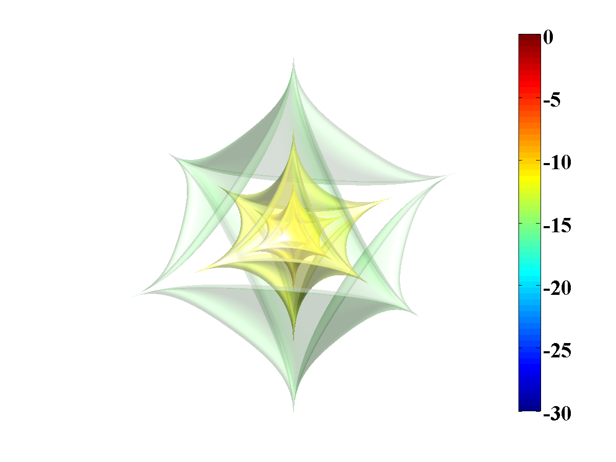
Figure 34: Predicted 3D gradient PDF in log-scale from our Model 1. Isosurfaces are shown for -14, -12, -10, and -8.

Since the GDP is stable with image contents, it is also valid on sub-images and image regions. As shown in Fig. 35(a,b), the gradient distribution is insensitive to the position, size, and shape of the patch. This is confirmed for an electron-microscopy image in Fig. 35(c,d). The image shows a transmission electron micrograph (ssTEM) of the Drosophila first instar larva ventral nerve cord (VNC) with a resolution of $4\times 4\times 50$ nm/pixel [Cardona et al., 2010]. The gradient distributions within manually segmented mitochondria and synapses (all regions pooled) are almost identical, as shown in Fig. 35(d). This suggests that the characteristic gradient distribution is maybe more of a function of the imaging process than of the imaged objects. It also shows how the GDP can be straightforwardly extended to multi-region methods.

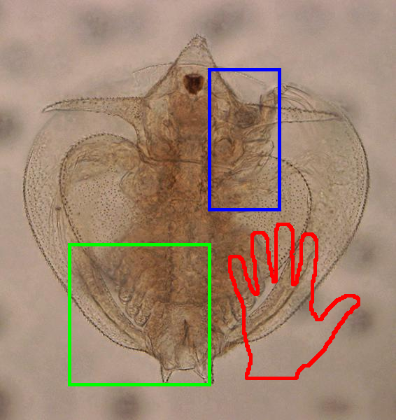
(a) Different local image patches.

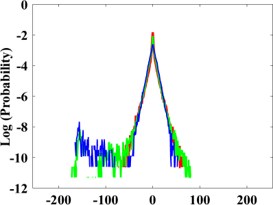
(b) Gradient distributions in these patches.

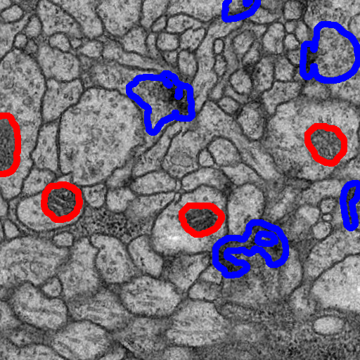
(c) Mitochondria (red) and synapses (blue) imaged by electron microscopy.

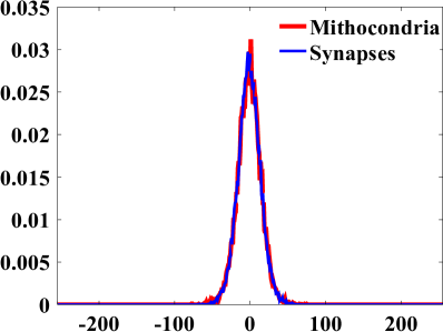
(d) Average gradient distributions.

Figure 35: Gradient distributions in local image regions are invariant, provided the regions are large enough.

Clearly, the GDP loses its validity when applied to small image patches that contain little or no internal structure. As the size of a local window decreases, we transition from a macroscopic view (entropy) to a microscopic view (pixel histogram). Since the GDP is a macroscopic quantity, it is only valid for large-enough image patches. But how large is large enough? Unfortunately, there is no sharp transition. To quantitatively see this, we define the naturalness map for a local window of edge length $w$ as:

$$N_{w}(x,y)=\iint p(\vec{G})\log\left(\frac{p(\vec{G})}{p^{\mathrm{pr}}}\right)\mathrm{d}G^{\hat{x}}\mathrm{d}G^{\hat{y}},$$ (42)

where $\hat{x}\in[x-w,x+w],\hat{y}\in[y-w,y+w]$. This quantifies the distance (KL-divergence) between the GDP and the gradient distribution in each local window. Computed for every image patch, this provides a map of how the image naturalness varies across patches. Two examples are shown in Fig. 36. When the window size decreases from 60 to 8, the average and median value of $N_{w}$ across all patches are plotted in Fig. 36(h,p). These plots show how the gradient distribution gradually diverges from the macroscopic GDP as the window size decreases. It seems that this behavior of prior invalidation is independent of image contents, as shown in Fig. 37. This is unexpected and requires further investigation.

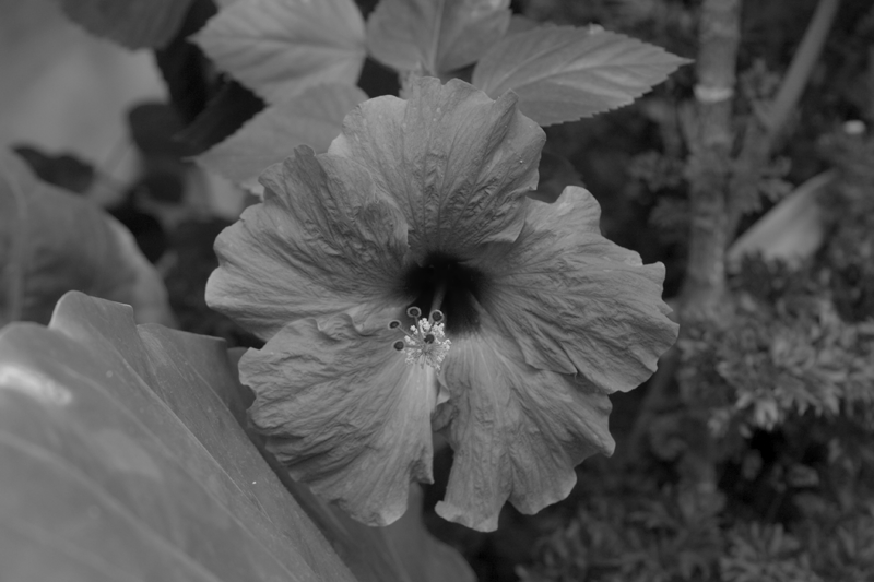
(a) original

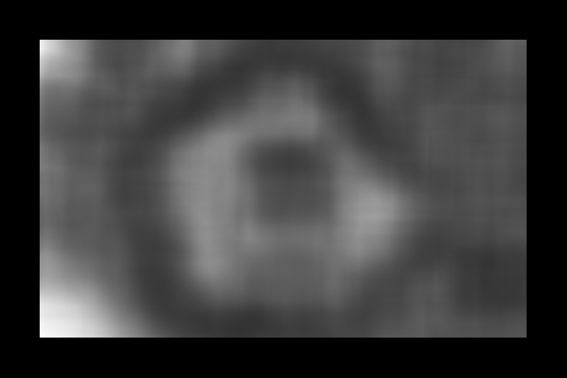
(b) $w=56$

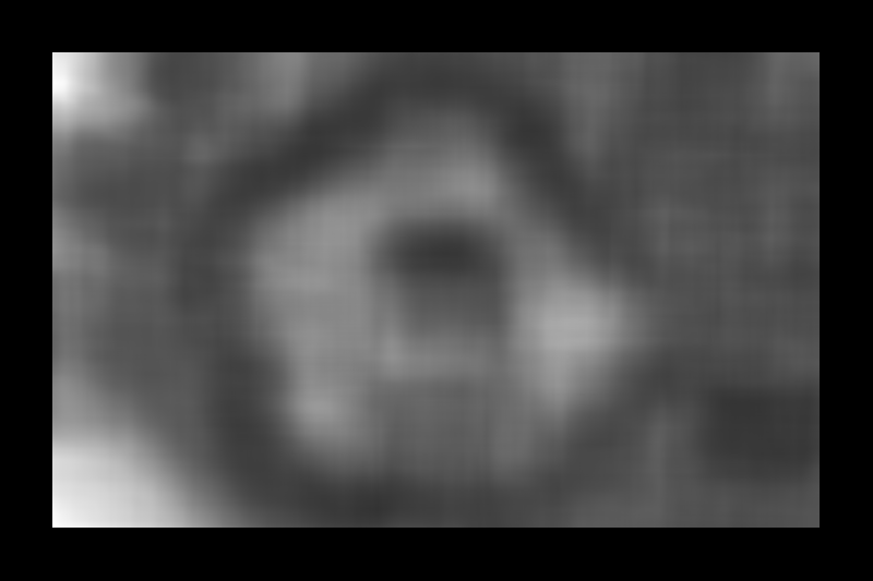
(c) $w=48$

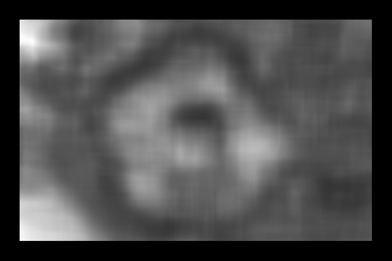
(d) $w=40$

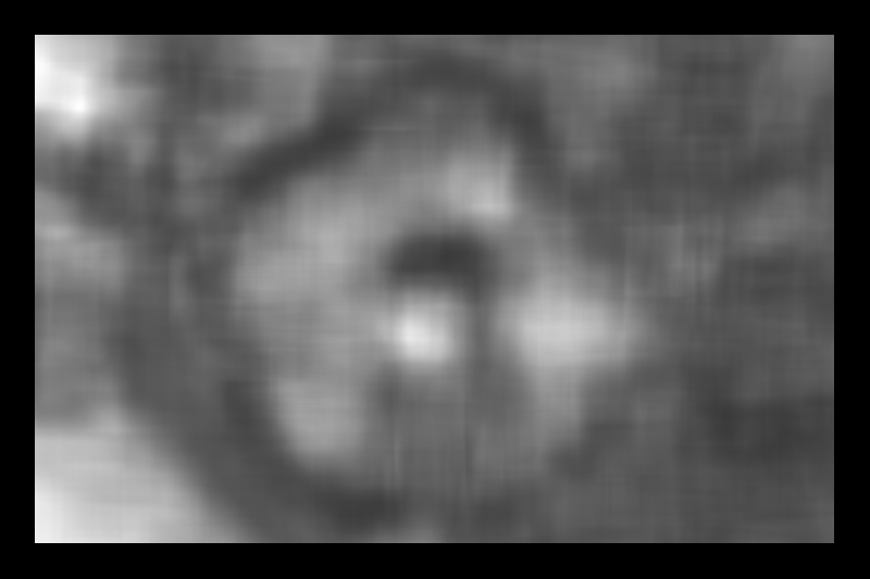
(e) $w=32$

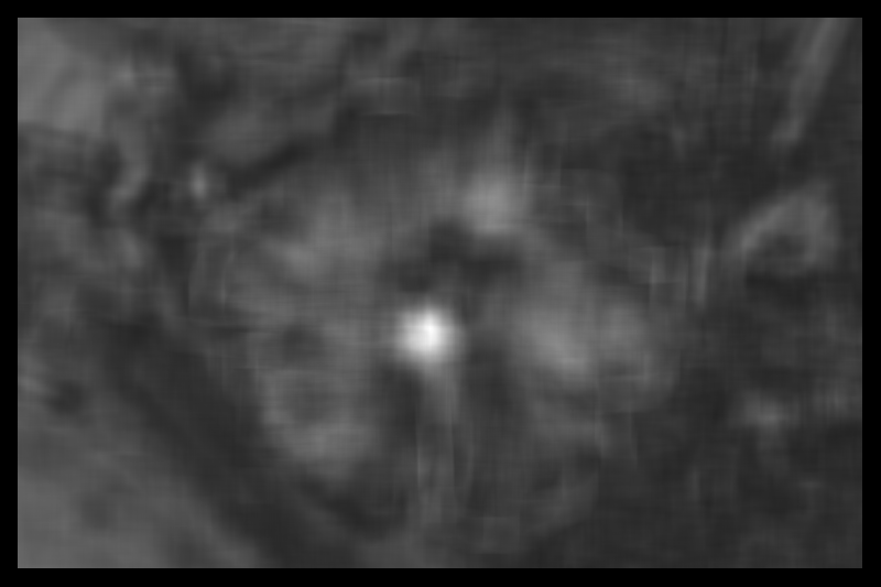
(f) $w=16$

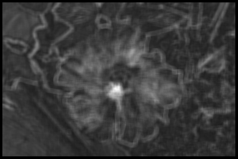
(g) $w=8$

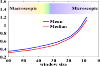
(h) $N_{w}$ average and median

(i) original

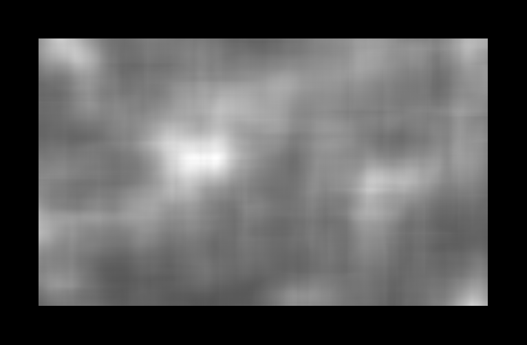
(j) $w=56$

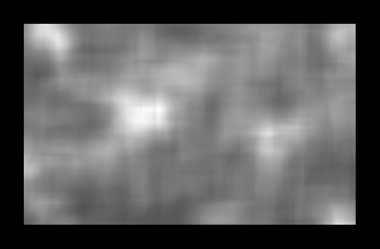
(k) $w=48$

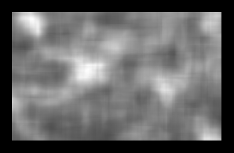
(l) $w=40$

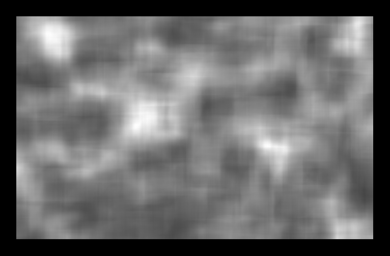
(m) $w=32$

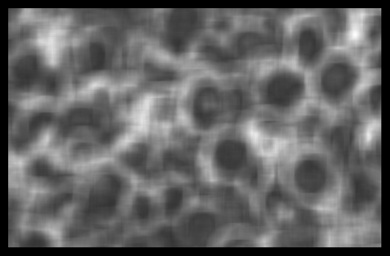
(n) $w=16$

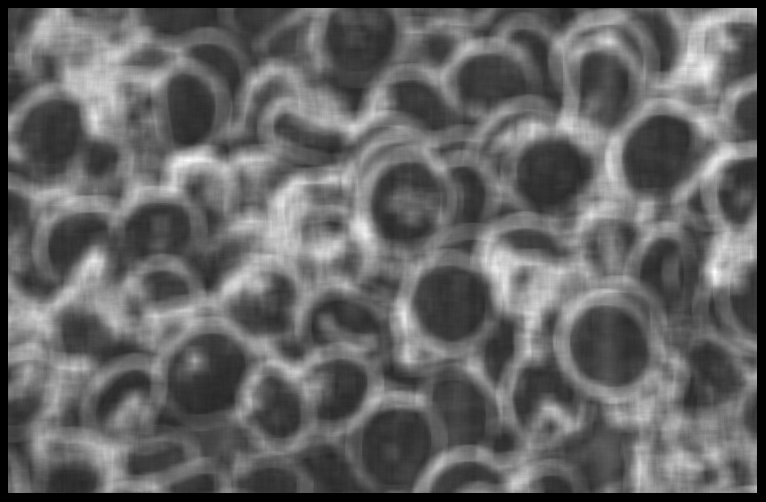
(o) $w=8$

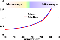
(p) $N_{w}$ average and median

Figure 36: Decreasing the local window size $w$, the gradient distribution prior increasingly differs from the empirical distribution within the windows. The original image is shown followed by naturalness maps computed in increasingly smaller moving window sizes $w$. The last panel shows how both the mean and the median distance $N_{w}$ between the GDP and all local windows gradually grow with decreasing window size $w$.

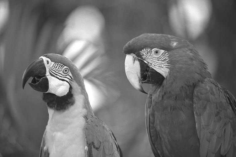
(a) parrots

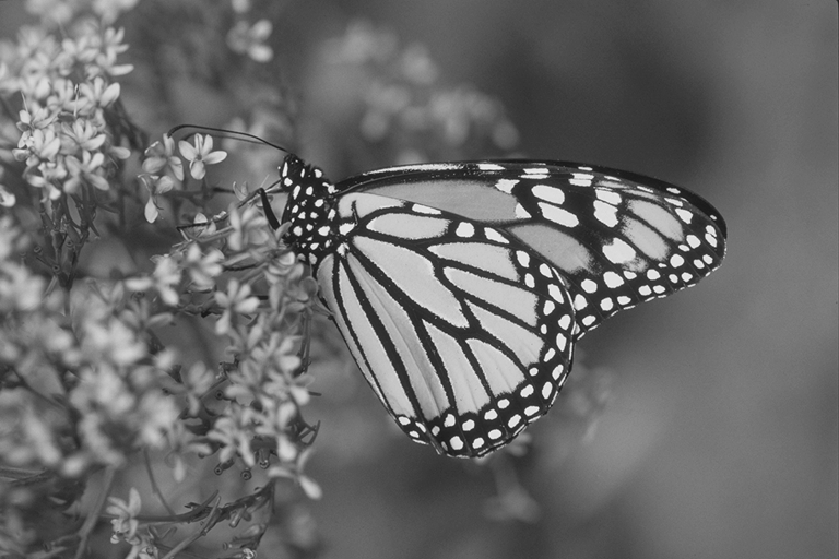
(b) monarch

(c) Lena

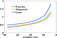
(d) $N_{w}$ average

Figure 37: Three examples suggesting that the behavior of $N_{w}$ with patch size is independent of image contents.

Notwithstanding the many open questions and limitations of gradient distribution priors, they have repeatedly proven extremely useful and competitive in image processing. The results presented here add to this. We believe, for the arguments set out here, that efficient parametric models of GDP learned from natural-scene images are a powerful and well-founded tool for biomedical image processing. In order to make this available to the community, we provide open-source code of all models presented here on our MOSAIC Group web page. We provide implementations in Matlab, C++ (included in the OpenCV library), and Java (as an ImageJ/Fiji plugin).

Appendix A Proof of Lemma 9.2

Proof.

Let $v=\|\nabla U\|_{2}^{2}$ and $W=T^{2}_{\mathrm{pr}}+\frac{b_{\mathrm{pr}}-v}{(b_{\mathrm{pr}}+v)^{2}}=0$. Then we have quadratic equation $T^{2}_{\mathrm{pr}}(b_{\mathrm{pr}}+v)^{2}+b_{\mathrm{pr}}-v=0$.

If $T^{2}_{\mathrm{pr}}b_{\mathrm{pr}}\geq\frac{1}{8}$, then $W\geq 0$.

If  $T^{2}_{\mathrm{pr}}b_{\mathrm{pr}}<\frac{1}{8}$, then $v_{L}=\frac{1-2T^{2}_{\mathrm{pr}}b_{\mathrm{pr}}-\sqrt{1-8T^{2}_{\mathrm{pr}}b_{\mathrm{pr}}}}{2T^{2}_{\mathrm{pr}}}$ and $v_{U}=\frac{1-2T^{2}_{\mathrm{pr}}b_{\mathrm{pr}}+\sqrt{1-8T^{2}_{\mathrm{pr}}b_{\mathrm{pr}}}}{2T^{2}_{\mathrm{pr}}}$ such that

$$\begin{cases}W<0&when~{}~{}v_{L}\leq v\leq v_{U}\\ W>0&otherwise\\ \end{cases}$$ (43)

∎

References

- Agrawal and Raskar [2007] Agrawal, A., Raskar, R., 2007. Gradient domain manipulation techniques in vision and graphics. ICCV short course .
- Awate and Whitaker [2006] Awate, S.P., Whitaker, R.T., 2006. Unsupervised, information-theoretic, adaptive image filtering for image restoration. IEEE Trans. Pattern Anal. Mach. Intell. 28, 364–376.
- Bae et al. [2012] Bae, H., Fowlkes, C.C., Chou, P.H., 2012. Patch mosaic for fast motion deblurring, in: in ACCV.
- Bhat et al. [2010] Bhat, P., Zitnick, C.L., Cohen, M., Curless, B., 2010. Gradientshop: A gradient-domain optimization framework for image and video filtering. ACM Trans. Graphics 29, 10.
- Biggs and Andrews [1997] Biggs, D.S.C., Andrews, M., 1997. Acceleration of iterative image restoration algorithms. Applied optics 36, 1766–1775.
- Boccardo et al. [1996] Boccardo, L., Gallouët, T., Orsina, L., 1996. Existence and uniqueness of entropy solutions for nonlinear elliptic equations with measure data. Annales de l’Institut Henri Poincare-Nonlinear Analysis 13, 539–552.
- Bredies et al. [2010] Bredies, K., Kunisch, K., Pock, T., 2010. Total generalized variation. SIAM Journal on Imaging Sciences 3, 492–526.
- Calder and Mansouri [2011] Calder, J., Mansouri, A.R., 2011. Anisotropic image sharpening via well-posed sobolev gradient flows. SIAM J. Math. Analysis 43, 1536–1556.
- Cao et al. [2011] Cao, X., Merwine, D.K., Grzywacz, N.M., 2011. Dependence of the retinal ganglion cell’s responses on local textures of natural scenes. J Vis 11. doi:10.1167/11.6.11.
- Cardona et al. [2010] Cardona, A., Saalfeld, S., Preibisch, S., Schmid, B., Cheng, A., Pulokas, J., Tomancak, P., Hartenstein, V., 2010. An integrated micro- and macroarchitectural analysis of the drosophila brain by computer-assisted serial section electron microscopy. PLoS Biol 8. doi:10.1371/journal.pbio.1000502.
- Chan et al. [2000] Chan, T., Marquina, A., Mulet, P., 2000. High-order total variation-based image restoration. SIAM J. Sci. Comput. 22, 503–516.
- Chan and Wong [1998] Chan, T.F., Wong, C.K., 1998. Total variation blind deconvolution. IEEE Transactions on Image Processing 7, 370–375.
- Chantas et al. [2010] Chantas, G., Galatsanos, N.P., Molina, R., Katsaggelos, A.K., 2010. Variational Bayesian image restoration with a product of spatially weighted total variation image priors. IEEE Trans. Image Proc. 19, 351–362.
- Chen et al. [2010] Chen, X., Yang, J., Wu, Q., 2010. Image deblur in gradient domain. Optical Engineering 49, 117003. doi:DOI10.1117/1.3505868.
- Chichilnisky [2001] Chichilnisky, E.J., 2001. A simple white noise analysis of neuronal light responses. Network 12, 199–213.
- Cho and Lee [2009] Cho, S., Lee, S., 2009. Fast motion deblurring. ACM Trans. Graphics 28, 145. doi:DOI10.1145/1618452.1618491.
- Cho et al. [2012] Cho, T.S., Zitnick, C.L., Joshi, N., Kang, S.B., Szeliski, R., Freeman, W.T., 2012. Image restoration by matching gradient distributions. IEEE Trans. Pattern Anal. & Machine Intell. (PAMI) 34, 683–694. doi:DOI10.1109/TPAMI.2011.166.
- Coltuc et al. [2006a] Coltuc, D., Bolon, P., Chassery, J., 2006a. Exact histogram specification. Ieee Transactions On Image Processing 15, 1143–1152. doi:DOI10.1109/TIP.2005.864170.
- Coltuc et al. [2006b] Coltuc, D., Bolon, P., Chassery, J.M., 2006b. Exact histogram specification. IEEE Transactions on Image Processing 15, 1143–1152.
- Dong et al. [2012] Dong, W., Feng, H., Xu, Z., Li, Q., 2012. Blind image deconvolution using the fields of experts prior. Optics Communications 285, 5051–5061. doi:DOI10.1016/j.optcom.2012.08.041.
- Donoho [2006] Donoho, D.L., 2006. Compressed sensing. Information Theory, IEEE Transactions on 52, 1289–1306.
- El-Fallah and Ford [1997] El-Fallah, A.I., Ford, G.E., 1997. Mean curvature evolution and surface area scaling in image filtering. IEEE Trans. Image Proc. 6, 750–753.
- Farbman et al. [2008] Farbman, Z., Fattal, R., Lischinski, D., Szeliski, R., 2008. Edge-preserving decompositions for multi-scale tone and detail manipulation. ACM Trans. Graph. 27, 67:1–67:10. doi:10.1145/1360612.1360666.
- Fattal [2009] Fattal, R., 2009. Edge-avoiding wavelets and their applications. ACM Trans. Graph. 28, 1–10. doi:http://doi.acm.org/10.1145/1531326.1531328.
- Fattal et al. [2002] Fattal, R., Lischinski, D., Werman, M., 2002. Gradient domain high dynamic range compression. ACM Trans. Graph. 21, 249–256.
- Fergus et al. [2006] Fergus, R., Singh, B., Hertzmann, A., Roweis, S.T., Freeman, W.T., 2006. Removing camera shake from a single photograph. ACM Trans. Graph. 25, 787–794.
- Gasso et al. [2009] Gasso, G., Rakotomamonjy, A., Canu, S., 2009. Recovering sparse signals with a certain family of nonconvex penalties and dc programming. Signal Processing, IEEE Transactions on 57, 4686–4698. doi:10.1109/TSP.2009.2026004.
- Gilboa et al. [2002] Gilboa, G., Sochen, N.A., Zeevi, Y.Y., 2002. Forward-and-backward diffusion processes for adaptive image enhancement and denoising. IEEE Transactions on Image Processing 11, 689–703.
- Goldstein and Osher [2009] Goldstein, T., Osher, S., 2009. The split Bregman method for L1-regularized problems. SIAM J. Imaging Sci. 2, 323–343.
- [30] Gollisch, T., Meister, M., . Eye smarter than scientists believed: Neural computations in circuits of the retina. Neuron 65, 150–164. URL: http://www.cell.com/neuron/abstract/S0896-6273(09)00999-4, doi:10.1016/j.neuron.2009.12.009.
- Gong et al. [2012] Gong, Y., Paul, G., Sbalzarini, I.F., 2012. Coupled signed-distance functions for implicit surface reconstruction, in: IEEE Intl. Symp. Biomed. Imaging (ISBI), pp. 1000–1003. doi:10.1109/ISBI.2012.6235726.
- Gong and Sbalzarini [2013] Gong, Y., Sbalzarini, I.F., 2013. Local weighted Gaussian curvature for image processing. Intl. Conf. Image Proc. (ICIP) , 534–538.
- Guillemot et al. [2012] Guillemot, T., Almansa, A., Boubekeur, T., 2012. Non local point set surfaces, in: 3D Imaging, Modeling, Processing, Visualization and Transmission (3DIMPVT), 2012 Second International Conference on, pp. 324 –331. doi:10.1109/3DIMPVT.2012.71.
- Gull and Skilling [1984] Gull, S., Skilling, J., 1984. Maximum entropy method in image processing. Communications, Radar and Signal Processing, IEE Proceedings F 131, 646–659.
- Gull and Daniell [1978] Gull, S.F., Daniell, G.J., 1978. Image reconstruction from incomplete and noisy data. Nature 272, 686–690. URL: http://dx.doi.org/10.1038/272686a0.
- Hamdi [2006] Hamdi, A., 2006. A modified bregman proximal scheme to minimize the difference of two convex functions. Applied Mathematics E-Notes [electronic only] 6, 132–140. URL: http://eudml.org/doc/55428.
- He et al. [2011] He, K., Sun, J., Tang, X., 2011. Single image haze removal using dark channel prior. Pattern Analysis and Machine Intelligence, IEEE Transactions on 33, 2341–2353. doi:10.1109/TPAMI.2010.168.
- Hu and Li [1991] Hu, J., Li, F., 1991. Maximum entropy image deconvolution in high resolution electron microscopy. Ultramicroscopy 35, 339 – 350.
- Hu and Yang [2012] Hu, Z., Yang, M.H., 2012. Good regions to deblur.
- Kazhdan et al. [2006] Kazhdan, M., Bolitho, M., Hoppe, H., 2006. Poisson surface reconstruction, in: Proc. 4th Eurographics Symp. Geometry Process., Eurographics Association. pp. 61–70.
- Kim [2006] Kim, S., 2006. PDE-based image restoration: A hybrid model and color image denoising. IEEE Trans. Image Proc. 15, 1163–1170.
- Krishnan and Fergus [2009] Krishnan, D., Fergus, R., 2009. Fast image deconvolution using hyper-Laplacian priors. Adv. Neural Inform. Proc. Sys. 22, 1–9.
- Krishnan et al. [2011] Krishnan, D., Tay, T., Fergus, R., 2011. Blind deconvolution using a normalized sparsity measure, in: CVPR, pp. 233–240.
- Lee and Seo [2005] Lee, S.H., Seo, J.K., 2005. Noise removal with Gauss curvature-driven diffusion. IEEE Trans. Image Proc. 14, 904–909.
- Levin et al. [2007] Levin, A., Fergus, R., Durand, F., Freeman, W.T., 2007. Deconvolution using natural image priors. Massachusetts Institute of Technology, Computer Science and Artificial Intelligence Laboratory .
- Li et al. [2012] Li, W., Li, Q., Gong, W., Tang, S., 2012. Total variation blind deconvolution employing split bregman iteration. J. Visual Communication and Image Representation 23, 409–417.
- Liu and Huang [2014] Liu, X., Huang, L., 2014. A new nonlocal total variation regularization algorithm for image denoising. Mathematics and Computers in Simulation 97, 224 – 233.
- Liu et al. [2011] Liu, X., Ying, Z., Qiu, S., 2011. A fourth-order partial differential equations method of noise removal, in: Image and Signal Processing (CISP), 2011 4th International Congress on, pp. 641–645. doi:10.1109/CISP.2011.6100378.
- Louchet and Moisan [2013] Louchet, C., Moisan, L., 2013. Posterior expectation of the total variation model: Properties and experiments. SIAM Journal on Imaging Sciences 6, 2640–2684.
- Lu et al. [2011] Lu, B., Wang, H., Lin, Z., 2011. High order Gaussian curvature flow for image smoothing, in: Multimedia Technology (ICMT), 2011 International Conference on, pp. 5888–5891. doi:10.1109/ICMT.2011.6001827.
- Marquina [2009] Marquina, A., 2009. Nonlinear inverse scale space methods for total variation blind deconvolution. SIAM J. Imaging Sciences 2, 64–83.
- McCann and Pollard [2008] McCann, J., Pollard, N.S., 2008. Real-time gradient-domain painting. ACM Trans. Graph. 27.
- Miller and Troyer [2002] Miller, K.D., Troyer, T.W., 2002. Neural noise can explain expansive, power-law nonlinearities in neural response functions. J Neurophysiol 87, 653–9.
- Nikolova et al. [2013] Nikolova, M., Wen, Y.W., Chan, R.H., 2013. Exact histogram specification for digital images using a variational approach. Journal of Mathematical Imaging and Vision 46, 309–325.
- Nishino et al. [2012] Nishino, K., Kratz, L., Lombardi, S., 2012. Bayesian defogging. International Journal of Computer Vision 98, 263–278. doi:DOI10.1007/s11263-011-0508-1.
- Paul et al. [2013] Paul, G., Cardinale, J., Sbalzarini, I.F., 2013. Coupling image restoration and segmentation: A generalized linear model/Bregman perspective. Int. J. Comput. Vis. .
- Pérez et al. [2003] Pérez, P., Gangnet, M., Blake, A., 2003. Poisson image editing, in: ACM Trans. Graph., ACM. pp. 313–318.
- Perona and Malik [1990] Perona, P., Malik, J., 1990. Scale-space and edge detection using anisotropic diffusion. IEEE Trans. Pattern Anal. & Machine Intell. (PAMI) 12, 629–639.
- Pillow et al. [2005] Pillow, J.W., Paninski, L., Uzzell, V.J., Simoncelli, E.P., Chichilnisky, E.J., 2005. Prediction and decoding of retinal ganglion cell responses with a probabilistic spiking model. J Neurosci 25, 11003–13. doi:10.1523/JNEUROSCI.3305-05.2005.
- Pustelnik et al. [2011] Pustelnik, N., Chaux, C., Pesquet, J., 2011. Parallel proximal algorithm for image restoration using hybrid regularization. IEEE Trans. Image Proc. 20, 2450–2462.
- Roth and Black [2009] Roth, S., Black, M.J., 2009. Fields of experts. IJCV 82, 205–229. doi:DOI10.1007/s11263-008-0197-6.
- Rudin et al. [1992] Rudin, L.I., Osher, S., Fatemi, E., 1992. Nonlinear total variation based noise removal algorithms. Physica D 60, 259–268.
- Shan et al. [2008] Shan, Q., Jia, J., Agarwala, A., 2008. High-quality motion deblurring from a single image. Acm Transactions On Graphics 27, 73. doi:DOI10.1145/1360612.1360672.
- Simoncelli and Olshausen [2001] Simoncelli, E.P., Olshausen, B.A., 2001. Natural image statistics and neural representation. Annual review of neuroscience 24, 1193–1216.
- Sundaramoorthi et al. [2007] Sundaramoorthi, G., Yezzi, A., Mennucci, A.C., 2007. Sobolev active contours. International Journal of Computer Vision 73, 345–366.
- Wang et al. [2004] Wang, Z., Bovik, A., Sheikh, H., Simoncelli, E., 2004. Image quality assessment: from error visibility to structural similarity. Image Processing, IEEE Transactions on 13, 600–612. doi:10.1109/TIP.2003.819861.
- Weiss and Freeman [2007] Weiss, Y., Freeman, W.T., 2007. What makes a good model of natural images?, in: CVPR, pp. 1–8. doi:10.1109/CVPR.2007.383092.
- Wong et al. [2011] Wong, A., Mishra, A., Zhang, W., Fieguth, P., Clausi, D.A., 2011. Stochastic image denoising based on markov-chain monte carlo sampling. Signal Processing 91, 2112–2120. doi:DOI10.1016/j.sigpro.2011.03.021.
- Xu and Wang [2009] Xu, D., Wang, R., 2009. An improved foe model for image deblurring. International Journal of Computer Vision 81, 167–171. doi:DOI10.1007/s11263-008-0155-3.
- Xu et al. [2011] Xu, L., Lu, C., Xu, Y., Jia, J., 2011. Image smoothing via L0 gradient minimization. ACM Trans. Graph. .
- Xu et al. [2012] Xu, L., Yan, Q., Xia, Y., Jia, J., 2012. Structure extraction from texture via relative total variation. ACM Trans. Graph. 31, 139:1–139:10. doi:10.1145/2366145.2366158.
- Zhang et al. [2012] Zhang, H., Zhang, Y., Li, H., Huang, T.S., 2012. Generative bayesian image super resolution with natural image prior. Ieee Transactions On Image Processing 21, 4054–4067. doi:DOI10.1109/TIP.2012.2199330.
- Zhang et al. [2011] Zhang, L., Zhang, L., Mou, X., Zhang, D., 2011. Fsim: A feature similarity index for image quality assessment. Ieee Transactions On Image Processing 20, 2378–2386. doi:DOI10.1109/TIP.2011.2109730.
- Zhu et al. [2007] Zhu, H., Shu, H., Zhou, J., Bao, X., Luo, L., 2007. Bayesian algorithms for PET image reconstruction with mean curvature and Gauss curvature diffusion regularizations. Computers in Biology and Medicine 37, 793–804.
- Zhu and Mumford [1997] Zhu, S., Mumford, D., 1997. Prior learning and Gibbs reaction-diffusion. IEEE Trans. Pattern Anal. & Machine Intell. (PAMI) 19, 1236–1250.