Algorithm xxx: RIDC Methods – A Family of Parallel Time-Integrators

Abstract

Revisionist integral deferred correction (RIDC) methods are a family of parallel–in–time methods to solve systems of initial values problems. The approach is able to bootstrap lower order time integrators to provide high order approximations in approximately the same wall clock time, hence providing a multiplicative increase in the number of compute cores utilized. Here we provide a library which automatically produces a parallel–in–time solution of a system of initial value problems given user supplied code for the right hand side of the system and a sequential code for a first-order time step. The user supplied time step routine may be explicit or implicit and may make use of any auxiliary libraries which take care of the solution of any nonlinear algebraic systems which may arise or the numerical linear algebra required.

Benjamin W. Ong, Ronald D. Haynes and Kyle Ladd, 2014. RIDC Algorithms: A Family of Parallel Time-Integrators

This work is supported by AFOSR Grant FA9550-12-1-0455, and NSERC Discovery grant (Canada).

Author’s addresses: R.  D. Haynes, Department of Mathematics and Statistics, Memorial University of Newfoundland; B. W. Ong, Mathematical Sciences, Michigan Technological University; K. Ladd, Barracuda Networks

1 Introduction

The fast, accurate solution of an initial-value problem (IVP) of the form

$${\bf y}^{\prime}(t)=f(t,{\bf y}),\quad{\bf y}(0)={\bf y}_{0},\quad t\in[0,T],$$ (1)

where ${\bf y}(t)\in\mathbb{C}^{N}$, $f:[\mathbb{R}\times C^{N}]\to\mathbb{C}^{N}$, is of practical interest in scientific computing. IVP (1) often arises from the spatial discretization of partial differential equations, and may require either an explicit or implicit time-integrator. The purpose of this software is to “wrap” a user-implemented first-order explicit or implicit solver for IVP (1) into a high-order parallel solver; that is, given $(t_{n},y_{n},f_{n})$, a user specifies a function that returns $(t_{n+1},y_{n+1},f_{n+1})$ using either a forward Euler or backward Euler integrator. This work differs from existing ODE integration software or libraries, where a user typically only needs to specify the system of ODEs and relevant problem parameters. The upside is that our software provides a parallel–in–time solution while giving the user complete control of the first-order time step routine. For example, the user may chose their own quality libraries for the solution of systems of nonlinear algebraic equations or efficient linear system solvers particularly tuned to the structure of their problems.

There are three general approaches for a time-parallel solution of IVPs [Burrage (1997)]. One approach is “parallelism-across-the-problem”, where a problem is decomposed into sub-problems that can be computed in parallel, and an iterative procedure is used to couple the sub-problems. Examples of this class of methods include parallel wave-form relaxation methods [Vandewalle and Roose (1989)]. The second approach is “parallel-across-the-step” methods, where the time domain is partitioned into smaller temporal subdomains which are solved simultaneously. Examples of this class of methods include parareal methods [Lions et al. (2001), Gander and Vandewalle (2007)], where the method alternates between applying a coarse sequential solver and a fine parallel solver. The third approach is “parallelism-across-the-method”, where one exploits concurrent function evaluations within a step to generate a parallel time integrator. This approach typically allows for small-scale parallelism, constrained by the number of function evaluations that can evaluated in parallel. This is often related to the order of the approximation. Examples of Runge–Kutta methods where stages can be evaluated in parallel include [Miranker and Liniger (1967), Enenkel and Jackson (1997), Ketcheson and bin Waheed (2014)]. Alternatively, one can use a predictor–corrector framework to generate parallel-across-the-method time integrators. This includes parallel extrapolation methods [Kappeller et al. (1996)], and RIDC integrators [Christlieb et al. (2010), Christlieb and Ong (2011)], which are the focus of this paper. A survey of parallel time integration methods has recently appeared [Gander (2015)].

1.1 Related Software

There are several well established software packages for solving differential algebraic equations, however not many of them are able to solve IVPs (1) in parallel. For sequential integrators, probably the most well known are MATLAB routines ode45, ode23, ode15s [Shampine et al. (1999)] to solve their systems of differential equations. These schemes use embedded RK pairs or numerical differentiation formulas (of the specified order) to approximate solutions to the differential equations using adaptive time-stepping. Readers might also be familiar with DASSL [Petzold (1983)], which implements backward differentiation formulas of order one through five. The nonlinear system at each time-step is solved by Newton’s method, and the resulting linear systems are solved using routines from LINPACK. DASSL leverages the SLATEC Common Mathematical Library [Vandevender and Haskell (1982)] for step-size adaptivity. Also popular are ODEPACK [Hindmarsh (1983)] and VODE [Brown et al. (1989)], a collection of fortran solvers for IVPs, SUNDIALS, a suite of robust time integrators and nonlinear solvers [Hindmarsh et al. (2005)], and there are a variety of ODE and DAE time steppers implemented in PETSc [Balay et al. (2014)] and GSL [Gough (2009)].

The selection of parallel solvers for IVPs is fairly sparse. EPPEER [Schmitt (2013)] is a Fortran95/OpenMP implementation of explicit parallel two-step peer methods [Weiner et al. (2008)] for the solution of ODEs on multicore architectures. PyPFASST [Emmett (2013)] is a python implementation of a modified parareal solver for ODEs and PDEs [Emmett and Minion (2012)]. XBRAID [Schroder et al. (2015)] is a C library that implements a multigrid-reduction-in-time algorithm [Falgout et al. (2014)], where multiple time-grids of different granularity are distributed across processors using MPI. PFASST++ [Emmett et al. (2015)] is a C++ implementation of the “ parallel full approximation scheme in space and time (PFASST) algorithm [Emmett and Minion (2014)]. There are other implementations (such as the dependency-driven parareal framework developed at Oakridge National Laboratory [Elwasif et al. (2011)]) that do not appear to be available for download at present.

2 Review of RIDC Methods

Spectral deferred correction (SDC) [Dutt et al. (2000)] provides an iterative correction of an approximate solution by solving an integral formulation of an error equation. This integral form stabilizes the classical differential deferred correction approach. RIDC is a re–formulation of SDC, pipelining successive calculations so that corrections can be obtained in parallel with an appropriate time lag. SDC, in contrast, is a sequential algorithm. Unlike the spectral deferred correction, which uses Gauss–Lobatto nodes, RIDC uses uniformly spaced nodes to minimize the memory footprint and to allow one to embed high order integrators [Christlieb et al. (2009), Christlieb et al. (2010)].

The basic idea of the IDC and RIDC approaches is to formulate associated error IVPs which correct numerical errors from the solutions to IVP (1); the parallelism arises from the ability to simultaneously compute solutions to both IVP (1) and solutions to the associated error IVPs. In this section, we review the formulation of the error equations, discretizations, and parallel properties of the RIDC algorithm. Please refer to [Christlieb et al. (2010), Christlieb and Ong (2011)] for accuracy and stability properties of the RIDC approach.

2.1 Error IVPs

Denote the (unknown) exact solution of IVP (1) as $y(t)$, and the approximate solution as $u(t)$, with $u(0)=y(0)$. The error in the approximate solution is $e(t)=y(t)-u(t)$. Define the residual (sometimes known as the defect) as $r(t)=u^{\prime}(t)-f(t,u)$. Then, the time derivative of the error satisfies

$$e^{\prime}(t)=y^{\prime}(t)-u^{\prime}(t)=f(t,u+e)-f(t,u)-r(t).$$

Since $e(0)=u(0)-y(0)=0$, we have just derived the associated error IVP. For stability, the integral form of the error IVP is preferred [Dutt et al. (2000)],

$$\left(e+\int_{0}^{t}r(\tau)\,d\tau\right)^{\prime}=f(t,u+e)-f(t,u).$$ (2)

Observing that the corrected approximation $u+e$ is still an approximation if the error equation (2) is solved numerically, we adopt a more general notation which will allow us to iteratively correct the solution until a desired accuracy is reached. Denote the initial approximation as $u^{[0]}$, the $p$th approximation as $u^{[p]}$, and the error to $u^{[p]}$ as $e^{[p]}$. Then, the error equation can be rewritten as

$$\left(e^{[p]}+\int_{0}^{t}r^{[p]}(\tau)\,d\tau\right)^{\prime}=f(t,u^{[p]}+e^{[p]})-f(t,u^{[p]}),$$ (3)

where $r^{[p]}=u^{[p]}(t)^{\prime}-f(t,u^{[p]})$.

2.2 Discretization

With some algebra, a first-order explicit discretization of (3), written in terms of the solution, gives

$$u_{n+1}^{[p+1]}=u_{n}^{[p+1]}+\Delta tf(t_{n},u_{n}^{[p+1]})-\Delta tf(t_{n},u_{n}^{[p]})+\int_{t_{n}}^{t_{n+1}}f(\tau,u^{[p]})\,d\tau.$$ (4)

Likewise a first-order implicit discretization of (3) gives

$$u_{n+1}^{[p+1]}=u_{n}^{[p+1]}+\Delta tf(t_{n+1},u_{n+1}^{[p+1]})-\Delta tf(t_{n+1},u_{n+1}^{[p]})+\int_{t_{n}}^{t_{n+1}}f(\tau,u^{[p]})\,d\tau.$$ (5)

In both semi-descretizations (4) and (5), a sufficiently accurate quadrature is needed to approximate the integrals present [Dutt et al. (2000)]. If a first order predictor was applied to obtain an approximate solution to (1), and first order correctors such as (4) and (5) are used, approximating the quadrature using

$$\int_{t_{n}}^{t_{n+1}}f(\tau,u^{[p]})\,d\tau\approx\begin{cases}\displaystyle\sum_{\nu=0}^{p+1}\alpha_{p\nu}f(t_{n+1-\nu},u_{n+1-\nu}^{[p]}),&\mbox{ if }n\geq p,\\ \displaystyle\sum_{\nu=0}^{p+1}\alpha_{p\nu}f(t_{\nu},u_{\nu}^{[p]}),&\mbox{ if }n<p,\end{cases},$$

where $\alpha_{p\nu}$ are quadrature weights,

$$\alpha_{p\nu}=\begin{cases}\displaystyle\int_{t_{n}}^{t_{n+1}}\prod_{i=0,i\neq\nu}^{p+1}\frac{(t-t_{n+1-i})}{(t_{n+1-\nu}-t_{n+1-i})}\,dt,&\mbox{ if }n\geq p,\\ \displaystyle\int_{t_{n}}^{t_{n+1}}\prod_{i=0,i\neq\nu}^{p+1}\frac{(t-t_{i})}{(t_{\nu}-t_{i})}\,dt,&\mbox{ if }n<p\end{cases}$$

results in a $P$th order method, if $(P-1)$ such corrections are applied.

2.3 Stability

A study of the (linear) stability of explicit RIDC methods is provided in [Christlieb et al. (2010)] and for implicit RIDC methods in [Christlieb and Ong (2011)]. The results indicate that the region of absolute stability of RIDC methods approach the region of absolute stability of the underlying predictor as the number of time steps increases. Moreoever, for the implicit RIDC4-BE method preserves the $A$–stability property of backward Euler.

2.4 Parallelization

As mentioned earlier, the parallelism arises from the ability to simultaneously compute solutions to both IVP (1) and solutions to the associated error IVPs (3). This is possible if there is some staggering to decouple solutions of IVP (1) and the error equations. As shown in Figure 1, staggering of one timestep is required to compute solutions in a pipeline parallel fashion. For example, while the predictor computes a solution at time $t_{10}$, the first corrector computes the correction at time $t_{9}$, the second corrector the second correction at time $t_{8}$, and so on.

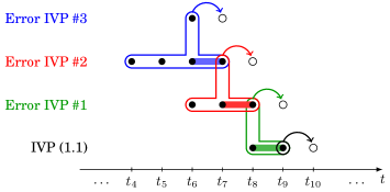
Figure 1: In a RIDC method, solution values and correction terms are computed in a pipeline fashion. For example, while a processor is computing a solution to IVP (1) at $t_{10}$, a second processor computes corrections to the numerical error at time $t_{9}$, a third processor computes additional corrections at time $t_{8}$, and so forth. (i.e., the open circles denote solutions that are simultaneously computed). The solid circles denote stored solution values that are needed for the quadrature approximation.

We discuss the “memory footprint” and the startup routine required by the RIDC method in Section 2.5 before presenting a pseudo algorithm for the RIDC methods on page 2.

2.5 Memory Footprint, Efficiency, Start-up and Shut-down

Figure 1 also shows the “memory footprint” required to execute the RIDC method in a pipeline-parallel fashion. The memory footprint are copies of the solution vector evaluated at earlier correction/prediction levels and time steps; one can also think of the memory footprint as the discretization stencil across the different correction and prediction levels. For a $P$th order RIDC method, the $(P-1)$st correction update (i.e. solving error IVP #(P-1)) requires a stencil of size $(P+1)$, the $(P-2)$nd correction requires an additional $(P-2)$ size stencil, the $(P-2)$nd correction requires an additional $(P-3)$ size stencil, and so on. The total memory footprint required for a $P$th order RIDC method is

$$\left(\sum_{i=1}^{P-1}(i+1)\right)+1=\frac{(P-1)(P)}{2}+(P-1)+1=\frac{P(P+1)}{2}.$$

In [Christlieb et al. (2010)] it is shown that the ratio of time steps taken by $P$th-order RIDC–Euler method, using $K$ steps before a restart, to the number of steps taken by the forward Euler method is

$$\gamma=1+\frac{(P-1)^{2}}{K}.$$

This shows that the method becomes more efficient (in terms of wall-clock time) as $K$ increases. One does have to balance a large value of $K$ with the possible increase in error this may cause. A study of this balance is provided in [Christlieb et al. (2010)].

Because of the staggering, start-up steps are needed to fill the memory footprint. As discussed in [Christlieb et al. (2010)], one should control the start-up steps to minimize the size of the memory footprint; that is, it is more desirable to stall the predictors and lower-level correctors initially (as appropriate) until all predictors and correctors can be marched in a pipeline fashion with the minimal memory footprint. For example, Figure 2 shows the start-up routine for a fourth-order RIDC method. Initially, only the predictor advances the solution from $t_{0}$ to $t_{1}$ in step one. In steps two and three, both the predictor and first corrector are advanced to populate the memory stencil in preparation for the second corrector. In step four, only the second corrector is advanced; the predictor and first corrector are stalled because the memory stencil needed to advance the second corrector from $t_{1}$ to $t_{2}$ is the same memory stencil needed to advance the corrector from $t_{0}$ to $t_{1}$.

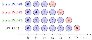
Figure 2: Start-up routine for a fourth-order RIDC method. Observe that the predictor and lower order correctors are occasionally stalled to ensure that a minimal memory footprint is used for the RIDC method. The fourth-order RIDC startup takes eight steps; from step nine on, the RIDC method can be marched in a pipeline fashion.

Although this concept is easy to grasp, the startup algorithm looks non-intuitive at first glance. Algorithm 1 specifies the nuts-and-bolts of the start-up routine. The RIDC method can be run in a pipe-line fashion (with the minimal memory footprint) after $startnum-1$ initialization steps, where $startnum=min(1,\frac{p(p+1)}{2}-1)$. For example, no initialization is required if $p=1$. If $p=4$, eight initialization steps are required – the RIDC method starts marching in a pipeline fashion at step nine.

$startnum=min(1,\frac{p(p+1)}{2}-1)$;

for $p=1$ to $(P-1)$ do

       march previous levels (i.e. $0,\ldots,(p-1)$) in a pipe for one step;

       march current level $(p-1)$ steps;

       march levels $0,\ldots,p$, in a pipe for one step;

      

end for

ALGORITHM 1 RIDC Startup-Routine

In the RIDC software, this startup routine is implemented using the $filter$ variable.

The shut-down routine for the RIDC method is straightforward; each predictor and corrector only advances the solution until the final time, $t_{F}$, is reached. The parallel RIDC pseudo-code is summarized in Algorithm 2.

fill memory stencil, compute $startnum$ ;

for $nt=startnum$ to $NT$ do

       for $p=0$ to $(P-1)$ do in parallel

             if $p=0$ then

                   use step to advance solution on prediction level (if $t_{F}$ not reached on prediction level);

                  

            else

                   use corr_fe or corr_be to advance solution on correction level $p$ (if $t_{F}$ not reached on correction level $p$);

                  

             end if

            

       end forpar

      update memory stencil ;

      

end for

ALGORITHM 2 RIDC Pseudo Code

3 RIDC Software

To utilize popular sequential integrators as described in Section 1.1, a user often specifies $f(t,y)$, the range of integration $[0,T]$, the initial condition $y_{0}=y(0)$ (and for DASSL, the derivative $y^{\prime}_{0}=y^{\prime}(0)$), and integrator parameters (such as parameters for controlling step-size adaptivity). While these general purpose time integration routines are convenient and easy to use, this “black-box” approach (for example, a user does not have to deal with the nonlinear solves arising from the backward differentiation formulas) sometimes precludes the use of additional information, such as the use of a problem-specific preconditioner, sparsity of the matrices, or multigrid iterative solvers.

The RIDC software presented here differs from the type of time-integration software mentioned above in that a first-order, user-specified, advance for $t\to t+\Delta t$ is bootstrapped to generate a high-order, parallel integrator using the integral deferred correction framework described in Section 2.

3.1 Installation Instructions for Users

The RIDC software is hosted at http://mathgeek.us/software.html. Users should download the latest libridc-x.x.tar.gz, and uncompress that file using the command tar -zxvf libridc-x.x.tar.gz.

There are no prerequisites for building the base RIDC software and examples in explicit/ and implicit/. To build the example in brusselator_gsl/, the GNU Scientific Library [Gough (2009)] and headers need to be installed. To build examples in implicit_mkl/, brusselator_mkl/ and brusselator_radau_mkl/, the Intel Math Kernel Library needs to be installed, and appropriate environment variables initialized.

In the top level directory ./configure --help gives the possible configuration options. To configure using standard build options type ./configure --prefix=/home/user/opt/libridc. The library is built by typing make && make check && make install. In this instance the library and required header files would be installed in home/user/opt/libridc/lib and home/user/opt/libridc/include respectively. By default, only the explicit and implicit examples are part of make check. Users can compile and check the MKL and GSL examples by typing --with-intel-mkl or --with-gsl in the configure step.

3.2 Installation Instructions for Developers

The development branch is hosted on GitHub, and can be obtained by issuing the instructions: git clone https://github.com/ongbw/ridc. The git commit correlating to this paper is f6c707e.

The RIDC software is managed by the GNU build system. As such, the developer release requires GNU autoconf, automake, libtool, m4, make and their respective prerequisites. If there are version mismatches between the RIDC software and the local system, issuing the commands autoreconf -f and automake -a -c should resolve version errors and warning. To build the documentation, Doxygen must be installed, as well as appropriate Doxygen pre-requisites. For example, to build a PDF manual documenting the source code, Doxygen requires a LaTeXcompiler.

3.3 Running the Examples

The directory examples/ includes five examples of utilizing the RIDC library, and one example, examples/brusselator_radau_mkl that implements a three stage, fifth-order Radau method to provide a basis of comparison with the RIDC integrators. Depending on the options selected in the ./configure step, some or all of these examples are built and run during during the make check process. Alternatively, a user can compile and run an example seperately after the ./configure step. For example, the subdirectory examples/explicit/ contains the code to solve

$$y_{i}^{\prime}=-(i+1)ty_{i},\,\,y_{i}(0)=1,\quad i=1,2,$$

using RIDC with an explicit Euler step function. To compile this specific example, move into the examples/explicit subdirectory and type make explicit. The executable explicit takes as input the order required and the number of time steps. For example ./explicit_ode1.exe 4 100 solves the system of ODEs using fourth order RIDC with 100 time steps. A shell script run.sh is provided to run the RIDC integrator with different numbers of time steps for a convergence study. A simple matlab or octave script convergence.m is included to test the order of convergence. octave convergence.m gives the slope and intercept for the linear fit of log of the error versus log of the time step. In this example we obtain a slope of $-4.0630$ indicating the we indeed have an order 4 method.

3.4 Using the RIDC library

To utilize the RIDC library, a main program should specify problem parameters (using the PARAMETER structure), initial values and the order of the RIDC integrator desired. The solution is integrated using a call to the ridc_fe or ridc_be functions The user also needs to specify template functions for the right hand side of the ODE $y^{\prime}=f(t,y)$ and a step function which advances the function from $t_{n}$ to $t_{n+1}$. This step routine may be complicated requiring large scale linear algebra provided by external external libraries or possibly a nonlinear solve. The examples/brusselator_gsl directory contains such an example. This example uses a backward Euler step for a nonlinear system of ODEs. The step function uses a Newton iteration (see the functions newt and jac) and the GNU scientific library (GSL) [Gough (2009)] to solve for the Newton step. The functions newt and jac required by step are defined and declared in brusselator.cpp. To link against the RIDC library, include the following arguments to the compilation command:

-L/home/user/opt/libridc/lib -I/home/user/opt/libridc/include -lridc

For information about the RIDC functions, please refer to the documentation located in doxygen-doc/ or online at http://mathgeek.us/software.html.

3.5 Under the hood

The RIDC software and examples are coded in C++; task parallelism is achieved using OpenMP threads to solve the predictors and the correctors in parallel. This mode of parallelism was chosen to accommodate the data movement/communication required by the RIDC algorithm when solving equations (4) and (5). We assume that the user-defined step routine to advance the solution is a first-order sequential integrator, although with some minor modifications to the RIDC software provided, bootstrapping higher order integrators is possible. The RIDC software can also be modified to leverage a thread-safe user-defined step routine, for example a CUDA-accelerated step routine [Ong et al. (2012)] or an MPI-parallelized step routine [Christlieb et al. (2012)] can be utilized, see Section 3.7. If the step routine uses an explicit Euler integrator, the RIDC software assumes that $u_{n+1}$ satisfies

$$u_{n+1}-u_{n}=\Delta tf(t_{n},u_{n}).$$

If the step routine uses an implicit Euler integrator, the RIDC software assumes that $u_{n+1}$ satisfies

$$u_{n+1}-u_{n}=\Delta tf(t_{n+1},u_{n+1}).$$

The RIDC software treats this step routine as a black box, as depicted in Figure 3.

Figure 3: User-defined step routine that advances a solution from $t_{n}$ to $t_{n+1}$.

The RIDC functions solve equations (4) and (5) by creating the necessary data structures to store copies of the solution vector described in Section 2.5, and then performing the appropriate algebraic computations on these stored solution values. First, consider the explicit Euler discretization of the error equation (4). Observe that $u_{n+1}^{[p+1]}$ can be constructed by applying the user-defined step routine to $u_{n}^{[p+1]}$ to obtain $\tilde{v}_{n+1}^{[p+1]}$, and then adding $-\Delta tf(t_{n},u_{n}^{[p]})+\int_{t_{n}}^{t_{n+1}}f(\tau,u^{[p]})\,d\tau$ to $\tilde{v}_{n+1}^{[p+1]}$ to finally obtain $u_{n+1}^{[p+1]}$. The explicit RIDC wrapper is displayed in Figure 4.

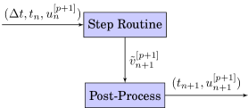
Figure 4: A visualization of the RIDC wrapper to obtain a solution to equation (4). The post process takes an input $\tilde{v}_{n+1}^{[p+1]}$ and returns $\tilde{v}_{n+1}^{[p+1]}-\Delta tf(t_{n},u_{n}^{[p]})+\int_{t_{n}}^{t_{n+1}}f(\tau,u^{[p]})\,d\tau$.

A similar observation can be made about the implicit Euler discretization of the error equation (5), however, one first constructs the intermediate value $\tilde{v}_{n}^{[p+1]}=u_{n}^{[p+1]}-\Delta tf(t_{n},u_{n}^{[p]})+\int_{t_{n}}^{t_{n+1}}f(\tau,u^{[p]})\,d\tau$, and then applies the user-defined step function to $\tilde{v}_{n}^{[p+1]}$. The implicit RIDC wrapper is displayed in Figure 5.

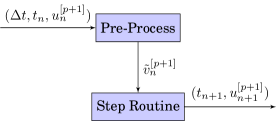
Figure 5: A visualization of the RIDC wrapper to obtain a solution to equation (5). The pre-process takes an input $u_{n}^{[p+1]}$ and returns $\tilde{u}_{n}^{[p+1]}-\Delta tf(t_{n},u_{n}^{[p+1]})+\int_{t_{n}}^{t_{n+1}}f(\tau,u^{[p]})\,d\tau$.

3.6 Discussion

The computational overhead of RIDC methods resides mainly in the quadrature approximation, and the subsequent linear combinations used to compute the corrected solutions. Provided this computational overhead is small compared to an evaluation of the step routine, good parallel speedup is achieved. In practice, this is almost always the case for implicit RIDC methods where solutions to linear equations, and/or Newton iterations are required. For explicit RIDC methods, good parallel speedup is only observed when the step routine is sufficiently expensive, such as in the computation of self-consistent forces for an $n$-body problem [Christlieb et al. (2010)].

As mentioned in Section 2.5, the RIDC method has to store copies of the solution vector evaluated at ealier correction/prediction levels. Although this memory requirement might appear restrictive, the memory footprint for high order single-step, multi-step or general linear methods are similar. Implicit RIDC methods also benefit from the loose coupling between the prediciton and corection equations; whereas a general implicit $s$-stage implicit RK method neccessitates the solution of a system of (potentially nonlinear) $sN$ equations, where $N$ are the number of differential algebraic equations. A $p$th-order RIDC method constructed using backward Euler integrators requires the solution of $p$ decoupled systems of $N$ (potentially nonlinear) algebraic equations.

3.7 Possible Generalizations

For clarity, only the simplest variant of the RIDC method (constructed using first order Euler integrators, uniform time-stepping, serial computation of the step routine) has been presented, and released as part of the base software version. Here, we make some remarks on how the base version of the software can be modified by the user to accommodate several generalizations discussed in this secton; indeed, the authors will release (when possible) modified versions of the software within the source repository that illustrate how to generate generalized RIDC integrators.

Step-size adaptivity for error control: In [Christlieb et al. (2014)], various variants of adaptive RIDC methods were presented. In the simplest variant, one uses standard error control stratagies to adaptively select step-sizes while solving IVP (1). These adaptively selected step-sizes are used for solving the error equations (2). To build step-size adaptivity into the provided RIDC software, the following modifications will be needed: (i) modify the time-loop appropriately to allow for non-uniform steps, (ii) modify the driver file appropriately to take a user-defined tolerance (as opposed to the number of time steps), (iii) recompute the integration matrix containing the quadrature weights at every time step. The user will presumably provide an additional adapt_step function, which takes as inputs the solution at time $t$, the previous time step used, $\Delta t_{old}$, a tolerance $tol$, and returns the time step selected, $\Delta t$, and the solution at the new time step, $t+\Delta t$.

Restarts: As discussed in [Christlieb et al. (2010)], the RIDC method accumulates error while running in a pipeline fashion – the most accurate solution does not propagate to the earlier prediction/correction levels. In some cases, it might be advantageous to stop the RIDC method, and use the most accurate solution to “restart” the computation. This requires only a simple modification to the main RIDC loop in ridc.cpp.

Constructing RIDC methods using higher-order integrators: With a few modifications, it is possible to use higher-order single step integrators within the RIDC software. The memory stencil, integration matrix and quadrature approximations will need to be modified in ridc.cpp.

Semi-implicit RIDC methods: Although semi-implicit RIDC methods have been constructed and studied in [Ong et al. (2012)], it is in general not possible to wrap a user-defined semi-implicit step function to solve the error equation (2). Consider the IVP

$${\bf y}^{\prime}(t)=f_{N}(t,{\bf y})+f_{S}(t,{\bf y}),$$

where $f_{S}$ contains stiff terms and $f_{N}$ contains the nonstiff terms. A first-order user-defined step function to solve this IVP would look like

$$u_{n+1}-u_{n}=\Delta tf_{N}(t_{n},u_{n})+\Delta tf_{S}(t_{n+1},u_{n+1}),$$

whereas the first-order IMEX discretization of the error equation (2) is

$$u_{n+1}^{[p+1]}=u_{n}^{[p+1]}+\Delta t\left[f_{N}(t_{n},u_{n}^{[p+1]})+f_{S}(t_{n+1},u_{n+1}^{[p+1]})\right]-\Delta t\left[f_{N}(t_{n},u_{n}^{[p]})+f_{S}(t_{n+1},u_{n+1}^{[p]})\right]$$

$$+\int_{t_{n}}^{t_{n+1}}\left[f_{N}(\tau,u^{[p]})+f_{S}(\tau,u^{[p]})\right]\,d\tau.$$

Althought it is not obvious how to automaticaly bootstrap a semi–implicit step function, a user can leverage the data structures and quadrature approximations in ridc.cpp to construct a new corr_fbe function, which should look similar in structure to the users’ step function.

Using accelerators for the step routine: Many computing clusters feature nodes with multiple accelerators, e.g. Nvidia GPGPUs or Intel Xeon Phis. If the user wishes to provide a step routine that is accelerated using these emerging architectures, the RIDC code can be modified to leverage multiple accelerators in a computational node. Modifications that are required include: adding an input variable “level” (an integer from 0 to $p-1$, where $p$ is the desired order / number of accelerators in the system) into the step routine, a function call within the step function to specify the appropriate accelerator, e.g. cudaSetDevice for the NVIDIA GPGPUs, and a modification of ridc.cpp so that the prediction/correction level is fed into the step function, ensuring that the linear algebra is performed on the appropriate accelerator.

Using distributed MPI for the step routine: Although the RIDC software can be modified to allow for an MPI-distributed step routine (provided this step-routine is thread safe), we showed in [Haynes and Ong (2014)] that a tighter coupling of the hybrid MPI-OpenMP formulation to reduce the number of messages is necessary for performance.

4 Numerical Experiment

The software includes several examples verifying that the RIDC methods attain their designed orders of accuracy. As mentioned, these examples also serve as templates for the user to bootstrap their own first order time integration methods to give a parallel–in–time approximation. Good parallel speedup is observed when the computational overhead for the RIDC methods (namely, the quadrature approximation and the linear combinations to compute the corrected solutions) is small compared to an evaluation of the step routine. Here, we present the numerical results for the Brusselator in $\mathbb{R}^{1}$.

$$u_{t} =A+u^{2}v-(B+1)u+\alpha u_{xx},$$ (6)

$$v_{t} =Bu-u^{2}v+\alpha v_{xx},$$

with $A=1$, $B=3$ and $\alpha=0.02$, initial conditions

$$u(0,x)=1+\sin(2\pi x),\qquad v(0,x)=3,$$

and boundary conditions

$$u(t,0)=u(t,1)=1,\qquad v(t,0)=v(t,1)=3.$$

A central finite difference approximation is used to discretize equation (6). The resulting nonlinear system of equations is solved using a Newton iteration. In the timing results, the Intel Math Kernel Library (MKL) is used to solve the linear system arising in each Newton iteration. The code for this example can be found in the examples/brusselator_mkl directory. Figure 6 shows a standard convergence study of error versus number of timesteps to demonstrate that the RIDC software bootstraps the first order integrator to generate a high-order method of the desired accuracy.

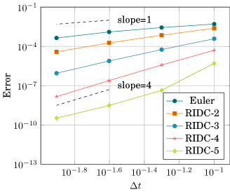
Figure 6: Standard convergence study of error versus time step, $\Delta t$, showing that RIDC methods achieve their designed orders of accuracy.

In Figure 7, the walltime used to compute each ridc method is plotted to show the “weak scaling” capability of RIDC methods. For example, the fourth-order RIDC method computes a solution using four computing cores that is 3-5 orders of magnitude more accurate than the first order Euler solution in approximately the same wallclock time. Tming results using a serial three-stage, fifth-order RADAU IIA integrator is also presented. A fifth order RIDC method (with five computing cores) provides a solution with comparable accuracy in 10% of the walltime. The scaling studies were performed on a single computational node consisting of a dual socket Intel E5-2670v2 chipset.

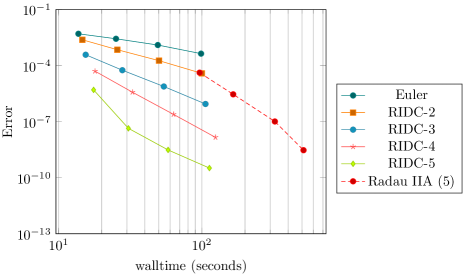
Figure 7: The error as a function of walltime is plotted for various RIDC methods. Here, two computing cores (set via OMP_NUM_THREADS=2) is used to compute the second order RIDC method (RIDC-2), three computing cores are used to compute RIDC-3, four computing cores are used to compute RIDC-4, and give compute cores are used to compute RIDC-5. A single computing core was used to compute Radau IIA. The RIDC software computes a $p$th order solution in approximately the same wall clock time as an Euler solution, provided $p$ computing cores are available. The parallel RIDC methods also provide good speedup over a serial Radau IIA integrator.

5 Conclusions

In this paper, we presented the revisionist integral deferred correction (RIDC) software for solving systems of initial values problems. The approach bootstraps lower order time integrators to provide high order approximations in approximately the same wall clock time, providing a multiplicative increase in the number of compute cores utilized. The C++ framework produces a parallel–in–time solution of a system of initial value problems given user supplied code for the right hand side of the system and the sequential code for a first-order time step. The user supplied time step routine may be explicit or implicit and may make use of any auxiliary libraries which take care of the solution of the nonlinear algebraic systems which arise or the numerical linear algebra required.

References

- [1]
- Balay et al. (2014) S Balay, S Abhyankar, M Adams, J Brown, P Brune, K Buschelman, V Eijkhout, W Gropp, D Kaushik, M Knepley, and others. 2014. PETSc Users Manual Revision 3.5. (2014).
- Brown et al. (1989) Peter N Brown, George D Byrne, and Alan C Hindmarsh. 1989. VODE: A variable-coefficient ODE solver. SIAM journal on scientific and statistical computing 10, 5 (1989), 1038–1051.
- Burrage (1997) Kevin Burrage. 1997. Parallel methods for ODEs. Advances in Computational Mathematics 7, 1 (1997), 1–3.
- Christlieb et al. (2012) Andrew Christlieb, Ronald Haynes, and Benjamin Ong. 2012. A Parallel Space-Time Algorithm. SIAM J. Sci. Comput. 34, 5 (2012), 233–248.
- Christlieb et al. (2010) Andrew Christlieb, Colin Macdonald, and Benjamin Ong. 2010. Parallel High-Order Integrators. SIAM J. Sci. Comput. 32, 2 (2010), 818–835.
- Christlieb et al. (2014) Andrew Christlieb, Colin Macdonald, Benjamin Ong, and Spiteri Raymond. in press, 2014. Revisionist Integral Deferred Correction with Adaptive Step-Size Control. (in press, 2014).
- Christlieb and Ong (2011) Andrew Christlieb and Benjamin Ong. 2011. Implicit parallel time integrators. J. Sci. Comput. 49, 2 (2011), 167–179. DOI:http://dx.doi.org/10.1007/s10915-010-9452-4
- Christlieb et al. (2009) Andrew Christlieb, Benjamin Ong, and Jing-Mei Qiu. 2009. Comments on High Order Integrators embedded within Integral Deferred Correction Methods. Comm. Appl. Math. Comput. Sci. 4, 1 (2009), 27–56.
- Christlieb et al. (2010) Andrew Christlieb, Benjamin Ong, and Jing-Mei Qiu. 2010. Integral Deferred Correction Methods constructed with high order Runge-Kutta integrators. Math. Comput. 79 (2010), 761–783.
- Dutt et al. (2000) Alok Dutt, Leslie Greengard, and Vladimir Rokhlin. 2000. Spectral deferred correction methods for ordinary differential equations. BIT 40, 2 (2000), 241–266.
- Elwasif et al. (2011) Wael Elwasif, Samantha Foley, David Bernholdt, Lee Berry, Debasmita Samaddar, David Newman, and Raul Sanchez. 2011. A dependency-driven formulation of parareal: parallel-in-time solution of PDEs as a many-task application. In Proceedings of the 2011 ACM international workshop on Many task computing on grids and supercomputers (MTAGS ’11). ACM, New York, NY, USA, 15–24. DOI:http://dx.doi.org/10.1145/2132876.2132883
- Emmett (2013) Matthew Emmett. 2013. PyPFASST: Parallel Full Approximation Scheme in Space and Time. (April 2013). http://pypfasst.readthedocs.org/en/latest
- Emmett et al. (2015) Matthew Emmett, Torbjorn Klatt, Robert Speck, and Daniel Ruprecht. 2015. parallel full approximation scheme in space and time. https://github.com/Parallel-in-Time/PFASST. (2015).
- Emmett and Minion (2012) Matthew Emmett and Michael Minion. 2012. Toward an efficient parallel in time method for partial differential equations. Comm. App. Math. and Comp. Sci 7, 1 (2012), 105–132.
- Emmett and Minion (2014) Matthew Emmett and Michael L Minion. 2014. Efficient implementation of a multi-level parallel in time algorithm. In Domain Decomposition Methods in Science and Engineering XXI. Springer, 359–366.
- Enenkel and Jackson (1997) Robert Enenkel and Kenneth Jackson. 1997. DIMSEMs - diagonally implicit single-eigenvalue methods for the numerical solution of stiff ODEs on parallel computers. Advances in Computational Mathematics 7, 1-2 (1997), 97–133. DOI:http://dx.doi.org/10.1023/A:1018986500842
- Falgout et al. (2014) RD Falgout, Stephanie Friedhoff, Tz V Kolev, SP MacLachlan, and Jacob B Schroder. 2014. Parallel time integration with multigrid. SIAM Journal on Scientific Computing 36, 6 (2014), C635–C661.
- Gander and Vandewalle (2007) Martin Gander and Stefan Vandewalle. 2007. On the superlinear and linear convergence of the parareal algorithm. Lecture Notes in Computational Science and Engineering 55 (2007), 291.
- Gander (2015) Martin J Gander. 2015. 50 Years of Time Parallel Time Integration. (2015).
- Gough (2009) Brian Gough. 2009. GNU scientific library reference manual. Network Theory Ltd., sales@network-theory.co.uk.
- Haynes and Ong (2014) Ronald Haynes and Benjamin Ong. 2014. A Hybrid MPI-OpenMP algorithm for the parallel space-time solution of Time Dependent PDEs. In Methods in Science and Engineering XXI, Lecture Notes in Computational Science and Engineering. Springer–Verlag, New York, 157–164.
- Hindmarsh (1983) Alan C Hindmarsh. 1983. ODEPACK, A Systematized Collection of ODE Solvers, RS Stepleman et al.(eds.), North-Holland, Amsterdam,(vol. 1 of), pp. 55-64. IMACS transactions on scientific computation 1 (1983), 55–64.
- Hindmarsh et al. (2005) Alan C Hindmarsh, Peter N Brown, Keith E Grant, Steven L Lee, Radu Serban, Dan E Shumaker, and Carol S Woodward. 2005. SUNDIALS: Suite of nonlinear and differential/algebraic equation solvers. ACM Transactions on Mathematical Software (TOMS) 31, 3 (2005), 363–396.
- Kappeller et al. (1996) M. Kappeller, M. Kiehl, M. Perzl, and M. Lenke. 1996. Optimized extrapolation methods for parallel solution of IVPs on different computer architectures. Appl. Math. Comput. 77, 2–3 (1996), 301 – 315. DOI:http://dx.doi.org/10.1016/S0096-3003(95)00219-7
- Ketcheson and bin Waheed (2014) David Ketcheson and Umair bin Waheed. 2014. A comparison of high-order explicit Runge–Kutta, extrapolation, and deferred correction methods in serial and parallel. Communications in Applied Mathematics and Computational Science 9, 2 (2014), 175–200.
- Lions et al. (2001) Jacques-Louis Lions, Yvon Maday, and Gabriel Turinici. 2001. A “parareal” in time discretization of PDEs. Comptes Rendus de l’Academie des Sciences Series I Mathematics 332, 7 (2001), 661–668.
- Miranker and Liniger (1967) Willard Miranker and Werner Liniger. 1967. Parallel methods for the numerical integration of ordinary differential equations. Math. Comp. 21 (1967), 303–320.
- Ong et al. (2012) Benjamin Ong, Andrew Christlieb, and Andrew Melfi. 2012. Parallel Semi-Implicit Time Integrators. Technical Report. Michigan State University. http://arxiv.org/pdf/1209.4297.pdf.
- Petzold (1983) Linda Petzold. 1983. A description of DASSL: a differential/algebraic system solver. In Scientific computing (Montreal, Que., 1982). IMACS, New Brunswick, NJ, 65–68.
- Schmitt (2013) Bernhard Schmitt. 2013. Peer methods for ordinary differential equations. (April 2013). http://www.mathematik.uni-marburg.de/~schmitt/peer/
- Schroder et al. (2015) Jacob Schroder, Robert Falgout, Tzanio Kolev, Ulrike Yang, Anders Petersson, Veselin Dobrev, Scott MacLachlan, Stephanie Friedhoff, and Ben O’Neil. 2015. XBraid: Parallel multigrid in time. http://llnl.gov/casc/xbraid. (2015).
- Shampine et al. (1999) Lawrence Shampine, Mark Reichelt, and Jacek Kierzenka. 1999. Solving index- DAEs in MATLAB and Simulink. SIAM Rev. 41, 3 (1999), 538–552 (electronic). DOI:http://dx.doi.org/10.1137/S003614459933425X
- Vandevender and Haskell (1982) Walter Vandevender and Karen Haskell. 1982. The SLATEC mathematical subroutine library. ACM SIGNUM Newsletter 17, 3 (1982), 16–21.
- Vandewalle and Roose (1989) Stefan Vandewalle and Dirk Roose. 1989. The parallel waveform relaxation multigrid method. In Parallel Processing for Scientific Computing, Proceedings of the Third SIAM Conference on Parallel Processing for Scientific Computing,. Soc. Indust. Appl. Math., Soc. Indust. Appl. Math., Philadelphia, PA, 152–156.
- Weiner et al. (2008) Rudiger Weiner, Katja Biermann, Bernhard A. Schmitt, and Helmut Podhaisky. 2008. Explicit two-step peer methods. Computers & Mathematics with Applications 55, 4 (2008), 609 – 619. DOI:http://dx.doi.org/10.1016/j.camwa.2007.04.026