Human Activity Learning and Segmentation using Partially Hidden Discriminative Models

Abstract

Learning and understanding the typical patterns in the daily activities and routines of people from low-level sensory data is an important problem in many application domains such as building smart environments, or providing intelligent assistance. Traditional approaches to this problem typically rely on supervised learning and generative models such as the hidden Markov models and its extensions. While activity data can be readily acquired from pervasive sensors, e.g. in smart environments, providing manual labels to support supervised training is often extremely expensive. In this paper, we propose a new approach based on semi-supervised training of partially hidden discriminative models such as the conditional random field (CRF) and the maximum entropy Markov model (MEMM). We show that these models allow us to incorporate both labeled and unlabeled data for learning, and at the same time, provide us with the flexibility and accuracy of the discriminative framework. Our experimental results in the video surveillance domain illustrate that these models can perform better than their generative counterpart, the partially hidden Markov model, even when a substantial amount of labels are unavailable.

1 Introduction

An important task in human activity recognition from low-level sensory data is segmenting the data streams and labeling them with meaningful sub-activities. The labels can then be used to facilitate data indexing and organisation, to recognise higher levels of semantics, and to provide useful context for intelligent assistive agents. The segmentation modules are often built on top of low-level sensor components which produce primitive and often noisy streams of events (e.g. see [7]). To handle the uncertainty inherent in the data, current approaches to activity recognition typically employ probabilistic models such as the hidden Markov models (HMMs) [14] and more expressive models, such as stochastic context-free grammars (SCFGs) [7], hierarchical HMMs (HHMMs) [6], abstract HMMs (AHMMs) [2], and dynamic Bayesian networks (DBNs).

All of these models are essentially generative, i.e. they model the relation between the activity sequence $y$ and the observable data stream $x$ via the joint distribution $p(y,x)$. Maximum likelihood learning with these models is then performed by finding a parameter that optimises the joint probability $p(y,x)$. This modeling approach has two drawbacks in general. Firstly, it is often difficult to capture complex dependencies in the observation sequence $x$, as typically, simplifying assumptions need to be made so that the conditional distribution $p(x|y)$ is tractable. This limits the choice of features that one can use to encode multiple data streams. Secondly, it is often advantageous to optimise the conditional distribution $p(y|x)$ as we do not have to learn the data generative process. Thirdly, as we are only interested in finding the most probable activity sequence $y^{*}=\arg\max_{y}p(y|x)$, it is more natural to model $p(y|x)$ directly.

Thus the discriminative model $p(y|x)$ is more suitable to specify how an activity $y$ would evolve given that we already observe a sequence of observations $x$. In other words, the activity nodes, rather than being the parents, become the children of the observation nodes. With appropriate use of contextual information, the discriminative models can represent arbitrary, dynamic long-range interdependencies which are highly desirable for segmentation tasks.

Moreover, whilst capturing unlabeled sensor data for training is cheap, obtaining labels in a supervised setting often requires expert knowledge and is time consuming. In many cases we are certain about some particular labels, for example, in surveillance data, when a person enters a room or steps on a pressure mat. Other labels (e.g. other activities that occur inside the room) are left unknown. Therefore, it is more desirable to employ the semi-supervised approach. Specifically, we consider two recent discriminative models, namely, the undirected Conditional Random Fields (CRFs) [9], (Figure 1(b)) and the directed Maximum Entropy Markov Models (MEMMs) [11] (Figure 1(a)). As the original models are fully observed, we provide a treatment of incomplete data for the CRFs and the MEMMs. The EM algorithm [5] is presented for both the models although it is not strictly required for the CRFs.

We provide experimental results in the video surveillance domain where we compare the performance of the proposed models and the equivalent generative HMMs [15] (Figure 1(c)) in learning and segmenting human indoor movement patterns. Out of three data sets studied, a common behaviour is that the HMM is outperformed by the discriminative counterparts even when a large portion of labels are missing. Providing contextual features for the models increases the performance significantly.

The novelty of this paper lies in the first work on modeling human activity using partially hidden discriminative models. Although semi-supervised learning has been investigated for a while, much work has concentrated on unstructured data and classification. There has been little work on structured data and segmentation and how much labeling effort are needed.

The remainder of the paper is organised as follows. Section 2 reviews related work in human activity segmentation and background in CRFs and MEMMs and in semi-supervision. Section 3 describes the partially hidden discriminative models. The paper then describes implementation and experiments and presents results in Section 4. The final section summarises major findings and further work.

2 Related work

Hidden Markov models (HMMs) have been used to model simple human activities and human motion patterns [3, 1, 18]. More recent approaches have used more sophisticated generative models to capture the hierarchical structure of complex activities. The abstract hidden Markov model (AHMM) [2] is used in [10] to model human transportation patterns from outdoor GPS sensors, and in [12] to model human indoor motion patterns from sensors placed in mobile robots. Using the AHMM, multiple levels of semantics can be built on top of the HMMs allowing flexibility in modeling the evolution of activities across multiple levels of abstraction. To learn the parameters, the expectation maximisation (EM) algorithm can be used. However, these models are generative, and are not suitable to work with arbitrary or overlapping features in the data streams.

Discriminative models specify the conditional probability $p(y|x)$ without modeling the data $x$. Let $y=\{y_{i:n}\}$ and assume that the probability $p(y|x)$ is specified with respect to a graph $\mathcal{G}=(\mathcal{E},\mathcal{V})$, where each vertex $i\in\mathcal{V}$ represents a random variable $y_{i}$ and the edges $e\in\mathcal{E}$ encode the correlation between variables. The graph $\mathcal{G}$ can be undirected, as in the Conditional Random Fields (CRFs) [9] (Figure 1(b)) or directed as in the Maximum Entropy Markov Models (MEMMs) [11] (Figure 1(a)). The CRFs define the model as follows

$$p(y|x;\lambda)=\frac{1}{Z(x;\lambda)}\prod_{c}\Psi_{c}(y_{c},x;\lambda)$$ (1)

where $c$ is the clique defined by the structure of $\mathcal{G}$, $\Psi_{c}(y_{c},x;\lambda)$ is the potential function defined over the clique $c$, $\lambda$ are model parameters, and $Z(x;\lambda)=\sum_{y}\prod_{c}\Psi_{c}(y_{c},x;\lambda)$ is the normalisation factor.

We consider the chain structure CRFs for our labeling tasks (Figure 1(b)), that is $y=\{y_{1:T}\}$. The potential function becomes $\Psi_{t}(y_{t-1},y_{t},x;\lambda)$, which is then typically parameterised using the log-linear model $\Psi_{t}(y_{t-1},y_{t},x;\lambda)=\exp(\sum_{k}\lambda_{k}f_{k}(y_{t-1},y_{t},x)$. The functions $\{f_{k}(y_{t-1},y_{t},x)\}$ are the features that capture the statistics of the data and the semantics at time $t$. The parameters $\lambda$ are the weight associated with the features and are estimated through training.

The MEMM is a directed, local version of the CRFs (Figure 1(a)), in which each source state $j$ has a conditional distribution

$$p_{j}(y_{t}|x_{t};\lambda)=p(y_{t}|y_{t-1}=j,x_{t};\lambda)=\frac{1}{Z(x_{t},j)}\exp(\sum_{k}\lambda_{jk}f_{k}(x_{t},y_{t}))$$ (2)

where $\lambda_{jk}$ are parameters of the source state $y_{t-1}=j$. The MEMMs can also be considered as conditionally trained HMMs (e.g. see the difference between Figures 1(a,c)). Although CRFs solve the label bias problem associated with the local normalised MEMMs [9], we believe that the MEMMs are useful in learning and understanding activity patterns because they directly encode the temporal state evolution through the transition model $p(y_{t}|y_{t-1}=j,x_{t};\lambda)$.

Supervised learning in the CRFs and MEMMs typically maximises the conditional log-likelihood $\mathcal{L}(\lambda)=\log p(y|x;\lambda)$. Gradient-based methods [16] are considered the fastest up to now.

Partially hidden models have received significant attention recently. The partially hidden Markov model (PHMM) proposed in [15] (Figure 1(c)) addresses the similar partial labeling problem as ours and we will use this model to compare with our discriminative models. In [13], CRFs with a hidden layer are introduced but labels are never given for this layer, thus they are not concerned with how robust the model is with respect to amount of missing data. The idea of constrained inference is introduced in [8] but they do not address the learning problem as we do. The more recent work in [4] extends the work of [8] to learning and addresses the interactive labeling effort by users. The results, however, are difficult to generalise to non-interactive applications in a non-active learning fashion.

3 Partially hidden discriminative models

3.1 The models

(a) MEMM		(b) CRF		(c) PHMM

Figure 1: (a,b): The partially hidden discriminative models, and (c): partially hidden Markov models. Filled circles and bars are data observations, empty circles are hidden labels, shaded circles are the visible labels

In our partially hidden discriminative models, the label sequence $y$ consists of a visible component $v$ (e.g. labels that are provided manually, or are acquired automatically by reliable sensors) and a hidden part $h$ (labels that are left unspecified or those we are unsure). The joint distribution of all visible variables $v$ is therefore given as

$$p(v|x;\lambda)=\sum_{h}p(v,h|x;\lambda)=\sum_{h}p(y|x;\lambda)$$ (3)

CRFs. For the log-linear CRFs, we have

$$p(y|x;\lambda)=\frac{1}{Z(x)}\prod_{t}\exp(\sum_{k}\lambda_{k}f_{k}(y_{t-1},y_{t},x))$$ (4)

where $Z(x)=\sum_{y}\prod_{t}\exp(\sum_{k}\lambda_{k}f_{k}(y_{t-1},y_{t},x))$. In this case, the complexity of computing $p(v|x;\lambda)$ is the same as that of computing the partition function $Z(x)$ up to a constant. Note that $Z(x)$ has the sum-product form, which can be computed efficiently using a single forward pass.

MEMMs. As stated in Section 2, directed models like the MEMMs are important in activity modeling because they naturally encode the state transitions given the observations. Here we offer a slightly more general view of the MEMMs in that we define a single model for all source states rather than separate models for each source state as in (2). In addition, as the model is discriminative, we do not have to model the observation sequence $x$. Thus we are free to encode arbitrary information exacted from the whole sequence $x$ to the local distribution. In our implementation, this is realised by using a sliding window of size $s$ centred at the current time $t$ to capture the local context of the observation. The local distribution reads

$$p(y_{t}|\Omega_{t},y_{t-1};\lambda)=\frac{1}{Z(\Omega_{t},y_{t-1})}\exp(\sum_{k}\lambda_{k}f_{k}(\Omega_{t},y_{t-1},y_{t}))$$ (5)

where $\Omega_{t}=\{x_{(t-s_{1}):(t+s_{2})}\}$ is the context of size $s=s_{1}+s_{2}+1$, and the parameter set $\{\lambda_{k}\}$ is now shared across the states. This view of MEMMs reduces to the original model if the feature set $\{f_{k}(\Omega_{t},y_{t-1},y_{t})\}$ consists of only indicator functions of states. The new view thus enjoys the same probabilistic inference properties but the learning is slightly different from the MEMM as it incorporates the structural constraint via the shared parameters while the MEMMs learns each local classifiers independently. The use of contextual features reflects the fact that the the current activity $y_{t}$ is generally correlated with the past and the future of sensor data.

As the graphical model of the MEMMs forms a Markov chain conditioned on the observation $x$, the joint incomplete distribution is therefore

$$p(v|x;\lambda)=\sum_{h}\prod_{t}p(y_{t}|\Omega_{t},y_{t-1};\lambda)$$ (6)

Again, this is a sum-product case, which can be computed by a single forward pass.

3.2 Parameters learning

To learn the model parameters that are best explained by the data, we maximise the penalised log-likelihood

$$\Lambda(\lambda)=\mathcal{L}(\lambda)-\frac{1}{2\sigma^{2}}||\lambda||^{2}$$ (7)

where $\mathcal{L}(\lambda)=\log p(v|x;\lambda)$. The regularisation term is needed to avoid over-fitting when only limited data is available for training. For simplicity, the parameter $\sigma$ is shared among all dimensions and is selected experimentally.

As with incomplete data, an alternative to maximise the log-likelihood is using the EM algorithm [5] whose Expectation (E-step) is to calculate the quantity

$$Q(\lambda^{j},\lambda)=\sum_{h}p(h|v,x;\lambda^{j})\log p(h,v|x)$$ (8)

and the Maximisation (M-step) maximises the concave lower bound of the log-likelihood $Q(\lambda^{j},\lambda)-\frac{1}{2\sigma^{2}}||\lambda||^{2}$ with respect to $\lambda$. Unlike Bayesian networks, the log-linear models do not yield closed form solutions in the the M-step. However, as the function $Q(\lambda^{j},\lambda)$ is concave, it is still advantageous to optimise with efficient Newton-like algorithms.

CRFs. For the partially hidden CRFs, the gradient of incomplete likelihood reads

$$\frac{\partial\mathcal{L}(\lambda)}{\partial\lambda_{k}}=\sum_{t}\sum_{h_{t-1},h_{t}}p(h_{t-1},h_{t}|v,x;\lambda)f_{k}(h_{t-1},h_{t},v,x)-\sum_{t}\sum_{y_{t-1},y_{t}}p(y_{t-1},y_{t}|x;\lambda)f_{k}(y_{t-1},y_{t},x)$$ (9)

Zeroing the gradient does not yield an analytical solution, so typically iterative numerical methods such as conjugate gradient and Newton methods are needed. The gradient of the lower bound in the EM framework of (8) is similar to (9), except that the pairwise marginals $p(h_{t-1},h_{t}|v,x;\lambda)$ are now replaced by the marginals of the previous EM iteration $p(h_{t-1},h_{t}|v,x;\lambda^{j})$. The pairwise marginals $p(y_{t-1},y_{t}|x)$ can be computed easily using a forward pass and a backward pass in the standard message passing scheme on the chain. Details are omitted for space constraint.

MEMMs. In learning of MEMMs, the E-step is to calculate

$$Q(\lambda^{j},\lambda)=\sum_{t}\sum_{h_{t-1}}p(h_{t-1}|v,\Omega_{t};\lambda^{j})\sum_{h_{t}}p(h_{t}|h_{t-1},\Omega_{t};\lambda^{j})\log p(h_{t}|h_{t-1},\Omega_{t};\lambda)$$ (10)

and the M-step is to solve the zeroing gradient equation

$$\frac{\partial Q(\lambda^{j},\lambda)}{\partial\lambda_{k}}\left\{\right\} = \sum_{t}\sum_{h_{t-1}}p(h_{t-1}|v,\Omega_{t};\lambda^{j})A_{t}(h_{t-1})\,\,\mbox{where}$$

$$A_{t}(h_{t-1}) = \sum_{h_{t}}p(h_{t}|h_{t-1},\Omega_{t};\lambda^{j})f_{k}(h_{t-1},h_{t},\Omega_{t})-\sum_{y_{t}}p(y_{t}|h_{t-1},\Omega_{t};\lambda)f_{k}(h_{t-1},y_{t},\Omega_{t})$$

Computation of the EM reduces to that of marginals and state transition probabilities, which can be carried out efficiently in the Markov chain framework using dynamic programming.

3.3 Segmentation

For segmentation, we use the MAP assignment $y^{*}=\arg\max_{y}p(y|x,\lambda)$ to infer the most probable label sequence $y^{*}$ for a given data sequence $x$. For both the CRFs and MEMMs, the Viterbi algorithm [14] can be naturally adapted. If some labels are provided (e.g. by some reliable sensors, or by users in interactive applications) we have the so-called constrained inference [8], but this is a trivial adaptation of the Viterbi decoding [14].

3.4 Comparison with the PHMMs

The main difference between the models described in this section (Figure 1(a,b)) and the PHMMs [15] (Figure 1(c)) is the conditional distribution $p(y|x)$ in discriminative models compared to the joint distribution $p(y,x)$ in the PHMMs. The data distribution of $p(x)$ and how $x$ is generated are not of concern in the discriminative models. In the PHMMs, on the contrary, the observation point $x_{t}$ is presumably generated by the parent label node $y_{t}$, so care must be taken to ensure proper conditional independence among $\{x_{t}\}_{t=1}^{T}$. This difference has an implication that, while the discriminative models may be good to encode the output labels directly with arbitrary information extracted from the whole observation sequence $x$, the PHMMs better represent $x$ when little information is associated with $y$. For example, when $y$ is totally missing, $p(x)=\sum_{y}p(y,x)$ is still modeled in the PHMMs and provides useful information. Our experiments in the next section show this difference more clearly.

Moreover, whilst we employ the log-linear models with unconstrained parameters, the PHMMs use the constrained transition and emission probabilities as parameters. In terms of modeling label ‘visibility’, the PHMMs are more general as they allow a subset of labels to be associated with certain nodes, and not only a full set as in hidden nodes or a single label as in visible nodes. However, it is quite straightforward to extend our partially hidden discriminative models to incorporate the same representation.

4 Experiments and results

Our task is to infer the activity patterns of a person (the actor) in a video surveillance scene. The observation data is provided by static cameras while the labels, which are activities such as ‘go-from-A-to-B’ during the time interval $[t_{a},t_{b}]$ (see Table 1), are recognised by the trained models.

4.1 Setup and data

The surveillance environment is a $4\times 6m^{2}$ dining room and kitchen (Figure 2). Two static cameras are installed to capture the video of the actor making some meals. There are six landmarks which the person can visit during the meals: door, TV chair, fridge, stove, cupboard, and dining chair. Figure 2 shows the room and the special landmarks viewed from the two cameras.

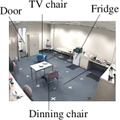
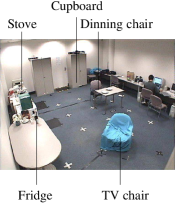
Figure 2: The environment and scene viewed from the two cameras.

Table 1: The primitive activities (the labels).

Activity	Landmarks	Activity	Landmarks
1	Door$\rightarrow$Cupboard	7	Fridge$\rightarrow$TV chair
2	Cupboard$\rightarrow$Fridge	8	TV chair$\rightarrow$Door
3	Fridge$\rightarrow$Dining chair	9	Fridge$\rightarrow$Stove
4	Dining chair$\rightarrow$Door	10	Stove$\rightarrow$Dining chair
5	Door$\rightarrow$TV chair	11	Fridge$\rightarrow$Door
6	TV chair$\rightarrow$Cupboard	12	Dining chair$\rightarrow$Fridge

We study three scenarios corresponding to the person making a short meal (denoted by SHORT_MEAL), having a snack (HAVE_SNACK), and making a normal meal (NORMAL_MEAL). Each scenario comprises of a number of primitive activities as listed in Table 1. Figure 3 shows the association between scenarios and their primitive activities. The SHORT_MEAL data set has 12 training and 22 testing video sequences; and each of the HAVE_SNACK and NORMAL_MEAL data sets consists of 15 training and 11 testing video sequences. For each raw video sequence captured, we use a background subtraction algorithm to extract a corresponding discrete sequence of coordinates of the person based on the person’s bounding box. The training sequences are partially labeled, indicated by the portion of missing labels $\rho$. The testing sequences provide the ground-truth for the algorithms. The sequence length ranges from $T=20-60$ and the number of labels per sequence is allowed to vary as $T*(1-\rho)$ where $\rho\in[0,100\%]$.

Figure 3: Associated primitive activities.

We apply standard evaluation metrics such as precision $P$, recall $R$, and the $F1$ score given as $F1=2*P*R/(P+R)$ on a per-token basis.

4.2 Feature design and contextual extraction

Features are crucial components of the model as they tie raw observation data with semantic outputs (i.e. the labels). The features need to be discriminative enough to be useful, and at the same time, they should be as simple and intuitive as possible to reduce manual labour. The current raw data extracted from the video contains only $(X,Y)$ coordinates. From each coordinate sequences, at each time slice $t$, we extract a vector of five elements from the observation sequence $g(x,t)=(X_{t},Y_{t},u_{X_{t}},u_{Y_{t}},s_{t}=\sqrt{u_{X_{t}}^{2}+u_{Y_{t}}^{2}})$, which correspond to the $(X,Y)$ coordinates, the $X$ & $Y$ velocities, and the speed, respectively. Since the extracted coordinates are fairly noisy, we use the average velocity measurement within a time interval of small width $w$, i.e. $u_{X_{t}}=(X_{t+w/2}-X_{t-w/2})/w$. Typically, these observation-based features are real numbers and are normalised so that they have a similar scale.

We decompose the feature set $\{f_{k}(y_{t-1},y_{t},x)\}$ into two subsets: the state-observation features

$$f_{l,m,\epsilon}(x,y_{t}):=\mathbb{I}[y_{t}=l]h_{m}(x,t,\epsilon)$$ (11)

and the state-transition features

$$f_{l_{1},l_{2}}(y_{t-1},y_{t}):=\mathbb{I}[y_{t-1}=l_{1}]\mathbb{I}[y_{t}=l_{2}]$$ (12)

where $m=1..5$ and $h_{m}(x,t,\epsilon)=g_{m}(x,t+\epsilon)$ with $\epsilon=-s_{1},..0,..s_{2}$ for some positive integers $s_{1}$, $s_{2}$. The state-observation features in (11) thus incorporate neighbouring observation points within a sliding window of width $s=s_{1}+s_{2}+1$. This is intended to capture the correlation of the current activity with past and future observations, and is a realisation of the temporal context $\Omega_{t}$ of the observations in (5). Thus the feature set has $K=5s|Y|+|Y|^{2}$ features, where $|Y|$ is the number of distinct label symbols.

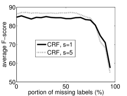
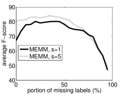
(a)		(b)

Figure 4: The role of context (SHORT_MEAL), $s$: the window size to extract observation data. (a) CRFs, (b) MEMMs. In all figures, the x-axis: the portion of missing labels (%) and the y-axis: the averaged F-score (%) over all states and over 10 repetitions.

To have a rough idea of how the observation context influences the performance of the models, we try different window sizes $s$ (see Equation (2)). The experiments show that incorporating the context of observation sequences does help to improve the performance significantly (see Figure 4). We did not try exhaustive searches for the best context size, nor did we implement any feature selection mechanisms. As the number of features scales linearly with the context size as $K=5s|Y|+|Y|^{2}$, where $s$ can be any integer between 1 and $T$, where $T$ is the sequence length, clearly a feature selection algorithm is needed when we want to capture long range correlation. For the practical purposes of this paper, we choose $s=5$ for both CRFs and MEMMs. Thus in our experiments, CRFs and MEMMs share the same feature set, making the comparison between the two models consistent.

4.3 Performance of models

To evaluate the performance of discriminative models against the equivalent generative counterparts, we implement the PHMMs (Figure 1(c)). The features extracted from the sensor data for the PHMMs include the discretised position and velocity. These features are different from those used in discriminative models in that discriminative features can be continuous.

To train discriminative models, we implement the non-linear conjugate gradient (CG) of Polak-Ribière and the limited memory quasi-Newton L-BFGS. After several pilot runs, we select the L-BFGS to optimise the objective function in Eq. (7) directly. In the case of MEMMs, the regularised EM algorithm is chosen together with the CG. The algorithms stop when the rate of convergence is less than $10^{-5}$. The regularisation constants are empirically selected as $\sigma=5$ in the case of CRFs, and $\sigma=20$ in the case of MEMMs.

For the PHMMs, it is observed that the initial parameter initialisation is critical to learn the correct model. Random initialisations often result in very poor performance. This is unlike the discriminative counterparts in which all initial parameters can be trivially set to zeros (equally important).

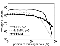
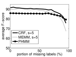
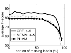
(a)	(b)	(c)

Figure 5: Average performance of models (a: SHORT_MEAL, b: HAVE_SNACK, c: NORMAL_MEAL). x-axis: portion of missing labels (%) and y-axis: the averaged F-score (%) over all states and 10 repetitions.

Table 2: The averaged precision ($P$) and recall ($R$) over all labels and over 10 repetitions. Top row contains missing portion $\rho$. The three scenarios: SM=SHORT_MEAL, HS=HAVE_SNACK, NM=NORMAL_MEAL.

Data	Model	Metric	0	10	20	30	40	50	60	70	80	90
SM	CRF	$P$	86.6	86.3	88.1	86.9	87.0	89.9	88.4	83.8	83.8	72.5
SM	CRF	$R$	87.4	87.1	88.1	87.7	87.4	91.3	90.1	81.6	82.5	68.5
SM	MEMM	$P$	81.7	87.8	87.0	84.2	85.2	83.1	81.2	80.5	73.2	57.0
SM	MEMM	$R$	83.4	88.4	87.5	84.2	86.1	82.7	81.5	75.8	67.8	55.2
SM	HMM	$P$	82.3	82.3	82.3	81.1	81.2	80.8	81.2	79.9	73.4	66.9
SM	HMM	$R$	83.2	83.2	83.2	83.7	84.1	83.3	84.1	83.1	75.7	70.9
HS	CRF	$P$	91.4	90.4	90.6	91.5	92.1	89.7	91.3	91.5	90.7	89.5
HS	CRF	$R$	92.4	91.5	90.1	90.6	91.7	90.0	91.9	91.5	91.1	88.8
HS	MEMM	$P$	89.9	88.9	90.8	89.2	91.5	88.7	89.6	89.4	85.1	80.0
HS	MEMM	$R$	91.2	90.3	91.4	89.5	93.7	90.4	91.3	91.0	87.7	81.4
HS	HMM	$P$	84.7	84.7	84.4	85.0	85.4	85.3	85.3	85.3	84.0	79.4
HS	HMM	$R$	88.5	88.5	88.1	87.2	87.6	87.3	87.3	87.3	87.4	83.4
NM	CRF	$P$	87.1	88.9	85.5	83.7	87.4	85.4	85.0	86.8	85.8	74.0
NM	CRF	$R$	83.5	88.5	81.8	80.7	86.6	85.7	81.5	86.3	84.9	72.8
NM	MEMM	$P$	85.4	85.0	84.6	83.5	84.8	81.9	77.9	78.3	75.0	62.0
NM	MEMM	$R$	81.7	82.1	81.3	81.0	84.9	81.4	78.4	79.7	76.9	62.6
NM	HMM	$P$	79.1	79.1	79.1	79.1	79.8	79.8	80.0	77.1	74.7	58.3
NM	HMM	$R$	80.4	80.4	80.4	80.4	81.3	81.3	81.6	79.5	78.0	63.8

Table 2 and Figure 5 show performance metrics (precision, recall and $F1$-score) of all models considered in this paper averaged over 10 repetitions. The three models have equivalent graphical structures. The CRFs and MEMMs share the same feature set but different from that of PHMMs. The generative PHMMs are outperformed by the discriminative counterparts in all cases given sufficient labels. This clearly matches the theoretical differences between these models in that when there are enough labels, richer information can be extracted in the discriminative framework, i.e. modeling $p(y|x)$ is more suitable. On the other hand, when only a few labels are available, the unlabeled data is important so it makes sense to model and optimise $p(x,y)$ as in the generative framework. On all data sets, the CRFs outperform the other models. These behaviours are consistent with the results reported in [9] in the fully observed setting. MEMMs are known to suffer from the label-bias problem [9], thus their performance does not match that of CRFs, although MEMMs are better than HMMs given enough training labels. In the HAVE_SNACK data set, the performance of MEMMs is surprisingly good.

A striking fact about the globally normalised CRFs is that the performance persists until most labels are missing. This is clearly a big time and effort saving for the labeling task.

5 Conclusions and further work

In this work, we have presented a semi-supervised framework for activity recognition on low-level noisy data from sensors using discriminative models. We illustrated the appropriateness of the discriminative models for segmentation of surveillance video into sub-activities. As more flexible information can be encoded using feature functions, the discriminative models can perform significantly better than the equivalent generative HMMs even when a large portion of the labels are missing. CRFs appear to be a promising model as the experiments show that they consistently outperform other models in all three data sets. Although less expressive than CRFs, MEMMs are still an important class of models as they enjoy the flexibility of the discriminative framework and enable online recognition as in directed graphical models.

Our study shows that primitive and intuitive features work well in the area of video surveillance. Semantically-rich and more discriminative contextual features can be realised through the technique of a sliding window. The wide context is especially suitable for the current problem because human activities are clearly correlated in time and space. However, to obtain the optimal context and to make use of the all information embedded in the whole observation sequence, a feature selection mechanism remains to be designed in conjunction with the models and training algorithms presented in this paper.

Although flat CRFs and MEMMs can represent arbitrarily high-level of activities, in many situations it may be more appropriate to structure the activity semantics into multiple layers or into a hierarchy. Future work will include models such as Dynamic Conditional Random Fields (DCRFs) [17], conditionally trained Dynamic Bayesian Networks and hierarchical model structures. A drawback of the log-linear models considered here is the slow learning curve compared to the traditional EM algorithm in Bayesian networks. It is therefore important to investigate more efficient training algorithms.

References

- [1] J. K. Aggarwal and Q. Cai. Human motion analysis: A review. Computer Vision and Image Understanding: CVIU, 73(3):428–440, 1999.
- [2] H. H. Bui, S. Venkatesh, and G. West. Policy recognition in the abstract hidden Markov model. Journal of Artificial Intelligence Research, 17:451–499, 2002.
- [3] Grzegorz Cielniak, Maren Bennewitz, and Wolfram Burgard. Where is …? Learning and utilizing motion patterns of persons with mobile robots. In Proceedings of the 18th International Joint Conference on Artificial Intelligence (IJCAI), pages 909–914, Acapulco, Mexico, August 2003.
- [4] Aron Culotta and Andrew McCallum. Reducing labeling effort for structured prediction tasks. In Proceedings of the National Conference on Artificial Intelligence (AAAI), 2005.
- [5] A. Dempster, N. Laird, and D. Rubin. Maximum likelihood from incomplete data via the EM algorithm. Journal of Royal Statistical Society, 39(1):1–38, 1977.
- [6] Shai Fine, Yoram Singer, and Naftali Tishby. The hierarchical hidden Markov model: Analysis and applications. Machine Learning, 32(1):41–62, 1998.
- [7] Y. Ivanov and A. Bobick. Recognition of visual activities and interactions by stochastic parsing. IEEE Transactions on Pattern Analysis and Machine Intelligence (PAMI), 22(8):852–872, August 2000.
- [8] Trausti Kristjannson, Aron Culotta, Paul Viola, and Andrew McCallum. Interactive information extraction with constrained conditional random fields. In Proceedings of the 19th National Conference on Artificial Intelligence (AAAI), pages 412–418, San Jose, CA, 2004.
- [9] J. Lafferty, A. McCallum, and F. Pereira. Conditional random fields: Probabilistic models for segmenting and labeling sequence data. In Proceedings of the International Conference on Machine learning (ICML), pages 282–289, 2001.
- [10] Lin Liao, Donald J Patterson, Dieter Fox, and Henry Kautz. Learning and inferring transportation routines. Artificial Intelligence, 171(5):311–331, 2007.
- [11] Andrew McCallum, Dayne Freitag, and Fernando Pereira. Maximum Entropy Markov models for information extraction and segmentation. In Proceedings of the 17th International Conference on on Machine Learning (ICML), pages 591–598. Morgan Kaufmann, San Francisco, CA, 2000.
- [12] Sarah Osentoski, Victoria Manfredi, and Sridhar Mahadevan. Learning hierarchical models of activity. In Proceedings of the IEEE/RSJ International Conference on Robots and Systems (IROS), 2004.
- [13] Ariadna Quattoni, Michael Collins, and Trevor Darrell. Conditional random fields for object recognition. In Lawrence K. Saul, Yair Weiss, and Léon Bottou, editors, Advances in Neural Information Processing Systems 17, pages 1097–1104. MIT Press, Cambridge, MA, 2005.
- [14] Lawrence R. Rabiner. A tutorial on hidden Markov models and selected applications in speech recognition. Proceedings of the IEEE, 77(2):257–286, 1989.
- [15] T. Scheffer and S. Wrobel. Active learning of partially hidden Markov models. In Active Learning, Database Sampling, Experimental Design: Views on Instance Selection, Workshop at ECML-2001/PKDD-2001, 2001.
- [16] Fei Sha and Fernando Pereira. Shallow parsing with conditional random fields. In Marti Hearst and Mari Ostendorf, editors, Proceedings of Human Language Technology (NAACL), pages 213–220, Edmonton, Alberta, Canada, May 27 - June 1 2003. Association for Computational Linguistics.
- [17] C.A. Sutton, K. Rohanimanesh, and A. McCallum. Dynamic Conditional Random Fields: factorized probabilistic models for labeling and segmenting sequence data. In Proceedings of the International Conference on Machine learning (ICML), 2004.
- [18] J. Yamato, J. Ohya, and K. Ishii. Recognizing human action in time-sequential images using hidden Markov models. In Proceedings of the IEEE Conference on Computer Vision and Pattern Recognition (CVPR), pages 379–385, 1992.