Chambers’s formula for the graphene and the Hou model with kagome periodicity and applications.

Abstract

The aim of this article is to prove that for the graphene model like for a model considered by the physicist Hou on a kagome lattice, there exists a formula which is similar to the one obtained by Chambers for the Harper model. As an application, we propose a semi-classical analysis of the spectrum of the Hou butterfly near a flat band.

1 Introduction

1.1 A brief historics

Starting from the middle of the fifties [11], solid state physicists have been interested in the flux effects created by a magnetic field (see in the sixties Azbel [4], Chambers [8]) . In 1976 a celebrated butterfly was proposed by D. Hofstadter [14] to describe as a function of the flux $\gamma$ the spectrum (at the bottom) of a Schrödinger operator with constant magnetic field and periodic electric potential. About ten years later mathematicians start to propose rigorous proofs for this approximation and to analyze the model itself. The celebrated ten martinis conjecture about the Cantor structure when $\gamma/2\pi$ is irrational was formulated by M. Kac and only solved a few years ago (see [2] and references therein). We refer also to the survey of J. Bellissard [5] for a state of the art in 1991. Once a semi-classical (or tight-binding) approximation is done, involving a tunneling analysis we arrive (modulo a controlled smaller error) in the case of a square lattice to the so-called Harper model, which is defined on $\ell^{2}(\mathbb{Z}^{2},\mathbb{C})$ by

$$(Hu)_{m,n}:=\frac{1}{2}(u_{m+1,n}+u_{m-1,n})+\frac{1}{2}e^{i\gamma m}u_{m,n+1}+\frac{1}{2}e^{-i\gamma m}u_{m,n-1}\,,$$

where $\gamma$ denotes the flux of the constant magnetic field through the fundamental cell of the lattice.
When $\frac{\gamma}{2\pi}$ is a rational, a Floquet theory permits to show that the spectrum is the union of the spectra of a family of $q\times q$ matrices depending on a parameter $\theta=(\theta_{1},\theta_{2})\in\mathbb{R}^{2}$.
More precisely, when

$$\gamma=2\pi p/q\,,$$ (1.1)

where $p\in\mathbb{Z}$ and $q\in\mathbb{N}^{*}$ are relatively prime, the two following matrices play an important role:

$$J_{p,q}={\rm diag}(e^{i(j-1)\gamma})\,,$$ (1.2)

and

$$(K_{q})_{jk}=1\;\mbox{ if }k\equiv j+1\,[q]\,,\,0\mbox{ else.}\,$$ (1.3)

In the case of Harper, the family of matrices is

$$M_{H}(\theta_{1},\theta_{2})=\frac{1}{2}(e^{i\theta_{1}}J_{p,q}+e^{-i\theta_{1}}J_{p,q}^{*}+e^{i\theta_{2}}K_{q}+e^{-i\theta_{2}}K_{q}^{*})\,.$$ (1.4)

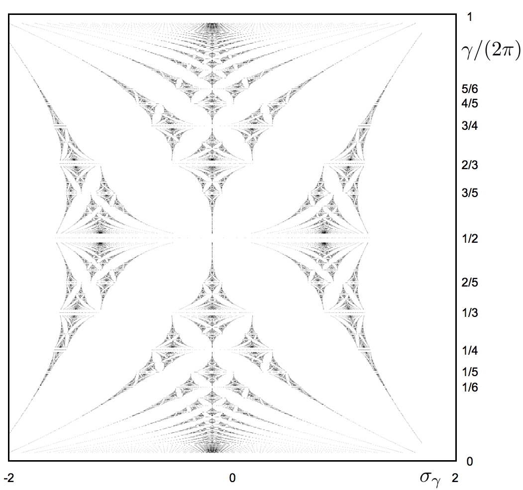
Figure 1: Square lattice.

The Hofstadter butterfly is then obtained as a picture in the rectangle $[-2,+2]\times[0,1]$ (see Figure 1). A point $(\lambda,\gamma/2\pi)$ is in the picture if there exists $\theta$ such that $\det(M_{H}(\theta_{1},\theta_{2})-\lambda)=0$ for some $\frac{p}{q}$ with $p/q\in[0,1]$ ($q\leq 50$).
The Chambers formula gives a very elegant formula for this determinant:

$$\det(M_{H}(\theta_{1},\theta_{2})-\lambda)=f^{H}_{p,q}(\lambda)+(-1)^{q}\left(\cos q\theta_{1}+\cos q\theta_{2}\right)\,,$$ (1.5)

where $f^{H}$ is a polynomial of degree $q$.

Many other models have been considered. In the case of a triangular lattice, the second model is, according to [16] (see also [3]),

$$M_{T}(\theta_{1},\theta_{2},\phi)=e^{i\theta_{1}}J_{p,q}+e^{-i\theta_{1}}J_{p,q}^{*}+e^{i\theta_{2}}K_{q}+e^{-i\theta_{2}}K_{q}^{*}+e^{i\phi}e^{i(\theta_{1}-\theta_{2})}J_{p,q}K_{q}^{*}+e^{-i\phi}e^{i(\theta_{2}-\theta_{1})}K_{q}J_{p,q}^{*}$$ (1.6)

with $\phi=-\gamma/2$.
The Chambers formula in this case takes the form

$$\det(M_{T}(\theta_{1},\theta_{2},\phi)-\lambda)=f^{T}_{p,q,\phi}(\lambda)+(-1)^{q+1}\left(\cos q\theta_{1}+\cos q\theta_{2}+\cos q(\theta_{2}-\theta_{1}-\phi)\right)\,.$$ (1.7)

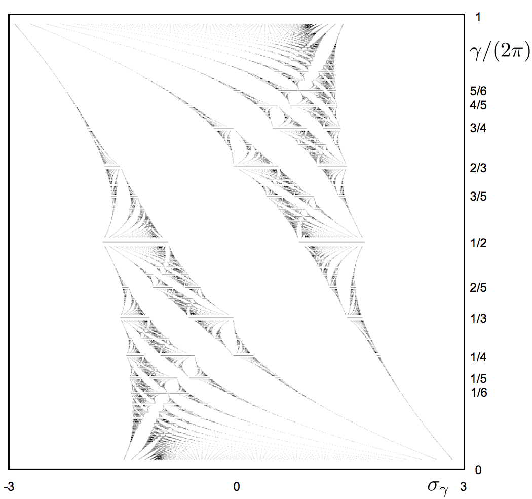
Figure 2: triangular lattice.

The resulting spectrum is given in Figure 2.

In the case of the hexagonal lattice, which appears also in the analysis of the graphene, we have to analyze

$$M_{G}(\theta_{1},\theta_{2}):=\left(\begin{array}[]{cc}0&I_{q}+e^{i\theta_{1}}J_{p,q}+e^{i\theta_{2}}K_{q}\\ I_{q}+e^{-i\theta_{1}}J_{p,q}^{*}+e^{-i\theta_{2}}K_{q}^{*}&0\end{array}\right)$$ (1.8)

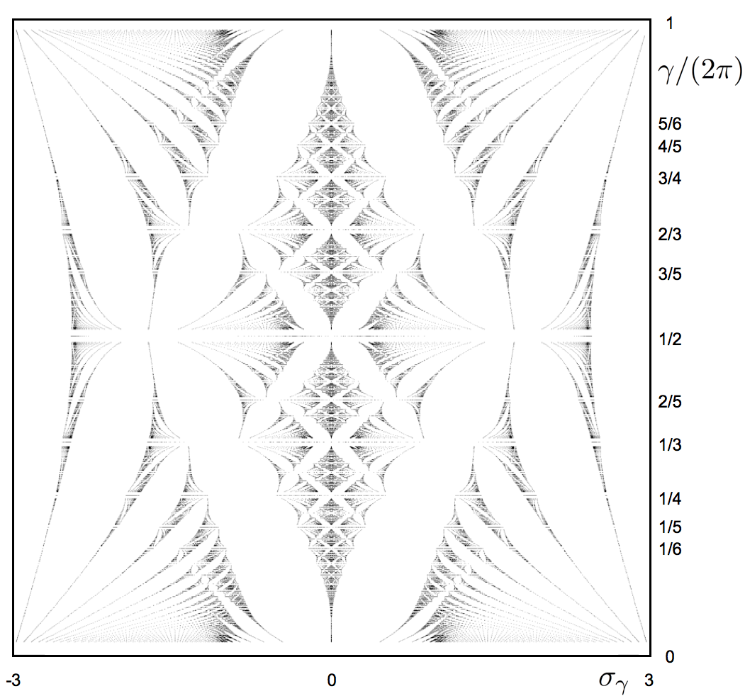
Figure 3: Hexagonal lattice.

We denote by $P_{G}$ the characteristic polynomial of $M_{G}$. The resulting spectrum is given in Figure 3.
Finally, inspired by the physicist Hou, P. Kerdelhué and J. Royo-Letelier [17] have shown that for the kagome lattice, the following approximating model is relevant: we consider the matrix

$$M_{K}(\theta_{1},\theta_{2},\omega)=\left(\begin{array}[]{ccc}0&A(\theta_{1},\theta_{2},\omega)&B(\theta_{1},\theta_{2},\omega)\\ A^{*}(\theta_{1},\theta_{2},\omega)&0&C(\theta_{1},\theta_{2},\omega)\\ B^{*}(\theta_{1},\theta_{2},\omega)&C^{*}(\theta_{1},\theta_{2},\omega)&0\end{array}\right)\,,$$ (1.9)

with

$$A(\theta_{1},\theta_{2},\omega) = e^{i(\omega+\frac{\gamma}{8})}(e^{-i\theta_{1}}J_{p,q}^{*}+e^{-i\frac{\gamma}{2}}e^{-i(\theta_{1}-\theta_{2})}J_{p,q}^{*}K_{q})$$

$$B(\theta_{1},\theta_{2},\omega) = e^{-i(\omega+\frac{\gamma}{8})}(e^{-i\theta_{1}}J_{p,q}^{*}+e^{-i\theta_{2}}K_{q}^{*})$$

$$C(\theta_{1},\theta_{2},\omega) = e^{i(\omega+\frac{\gamma}{8})}(e^{-i\frac{\gamma}{2}}e^{i(\theta_{1}-\theta_{2})}J_{p,q}K_{q}^{*}+e^{-i\theta_{2}}K_{q}^{*})\,.$$

Here $\omega$ is a parameter appearing in the model (most of the physicists consider without justification the case $\omega=0$). We refer to [17] for a discussion of this point.

The trigonometric polynomial

$$(x,\xi)\mapsto p^{\triangle}(x,\xi)=\cos x+\cos\xi+\cos(x-\xi)$$ (1.10)

which was playing an important role in the analysis of the triangular Harper model (see Claro-Wannier [9] and Kerdelhué [16]) will also appear in our analysis.
We denote by $P_{K}(\theta_{1},\theta_{2},\omega,\lambda)$ the characteristic polynomial $\det(M_{K}(\theta_{1},\theta_{2},\omega)_{\lambda})$.

1.2 Main results

The aim of this article is to prove that, for a model considered by Hou [15], there exists a formula which is similar to the one obtained by Chambers [8] for the Harper model. (see also Helffer-Sjöstrand [12], [13], Bellissard-Simon [7], C. Kreft [18], I. Avron (and coauthors) [3]). Such an existence was motivated by computations of [17]. We also consider the case of the graphene, where a huge litterature in Physics exists (see [10] and references therein) which is sometimes unaware of semi-classical mathematical results of the nineties. Note that the Chambers formula plays an important role in the semi-classical analysis of the Harper’s model (see for example [13]).

The first statement is probably well known in the physical literature.

Theorem 1.1 (Graphene).

$$P_{G}(\theta_{1},\theta_{2},\lambda)=(-1)^{q}\,{\rm det}(M_{T}(\theta_{1},\theta_{2},0)+3-\lambda^{2})\,.$$ (1.11)

The second statement was to our knowledge unobserved.

Theorem 1.2 (Kagome).

For any $\omega$, there exists a polynomial $Q_{\omega}$ of degree $3q$, with real coefficients, depending on $p,q$, such that

$$P_{K}(\theta_{1},\theta_{2},\omega,\lambda)=Q_{\omega}(\lambda)+2p^{\triangle}(q(\theta_{1}+p\pi),q(\theta_{2}+p\pi))R_{\omega}(\lambda)\,,$$ (1.12)

with

$$R_{\omega}(\lambda):=\left(\lambda+2\cos(3\omega-\frac{\gamma}{8})\right)^{q}\,.$$ (1.13)

Moreover the principal term of $Q_{\omega}(\lambda)$ is $\lambda^{3q}$.

We call $k$-th band the set described when $(\theta_{1},\theta_{2})\in\mathbb{R}^{2}$ by the $k$-th eigenvalue of the matrix $M_{K}$. We will call this band flat if this $k$-th eigenvalue is independent of $(\theta_{1},\theta_{2})$.

Corollary 1.3.

A flat band exists if and only if

$$Q_{\omega}(-2\cos(3\omega-\frac{\gamma}{8}))=0\,.$$

Remark 1.4.

• $Q_{\omega}$ is a trigonometric potential in $3\omega$.

• For $(p,q)$ given, the set of the $\omega$’s such that a flat band exists is discrete. Formula (1.9) shows indeed that the expression $P_{K}(\theta_{1},\theta_{2},\omega,-2\cos(3\omega-\gamma/8))$, which according to Theorem 1.2 is independent of $(\theta_{1},\theta_{2})$, takes the form $\Sigma_{j=-9q}^{9q}a_{j}e^{ij\omega}$ with $a_{9q}=e^{-i\frac{3\gamma q}{8}}$.

1.3 Examples

Let us illustrate by some examples mainly extracted of [17].
In the case when $q=1$ and $p=0$, one finds, for the Hou’s model:

$$P_{K}(\theta_{1},\theta_{2},\omega,\lambda)=\lambda^{3}-6\lambda-4\cos(3\omega)-2\left(\lambda+2\cos(3\omega)\right)p^{\triangle}(\theta_{1},\theta_{2})\,.$$

Hence, we have in this case:

$$Q_{\omega}(\lambda)=\lambda^{3}-6\lambda-4\cos(3\omega)\,.$$

It is then natural to ask if the two polynomial have a common zero. The condition reads:

$$Q_{\omega}(-2\cos(3\omega)\ )=0\,.$$

We get:

$$(\cos 3\omega)^{3}-\cos 3\omega=0\,,$$

hence $\cos 3\omega=0$ or $\cos 3\omega=\pm 1$. So a ”flat band” appears when $\omega=0$, which was mostly considered in the physical literature. Note that in [17], it is proved only that $\omega\rightarrow 0$ as a function of the initial semi-classical parameter. The set of $\omega$’s for which we have a flat band is $\{\omega_{k}=k\frac{\pi}{6}\,,\,k\in\mathbb{Z}\}\,.$

Another example is, as shown in [17] (Proposition 1.13), for $\omega=\pi/8$ and $p/q=3/2$. The bands are $\{-2\}$ (with multiplicity $2$), $[1-\sqrt{6},1-\sqrt{3}]$, $[1-\sqrt{3},1]$, $[1,1+\sqrt{3}]$ and $[1+\sqrt{3},1+\sqrt{6}]$.

1.4 Organization of the paper

This paper is organized as follows. In Section 2 we establish symmetry properties of the two matrices $J_{p,q}$ and $K_{q}$. In Section 3 we recall how a method due to Bellissard-Simon permits to establish the Chambers formula for a square lattice or a triangular lattice. In Section 4, we give an application to the case of the graphene. Section 5 is devoted to the proof of the main theorem for the kagome lattice. In Section 6, we establish the non overlapping of the bands in the case of the kagome lattice. Section 7 gives as an application a semi-classical analysis near a flat band and we finish with a conclusion.

2 Symmetries

We recall some basic symmetry properties of the two matrices $J_{p,q}$ and $K_{q}$. Some of them were used in the previous literature, some other are new. We first recall that

$$J_{p,q}K_{q}=\exp(-2i\pi\frac{p}{q})\,K_{q}J_{p,q}\,.$$ (2.1)

and (take the complex conjugation and the adjoint )

$$K_{q}^{*}J_{p,q}=\exp(-2i\pi\frac{p}{q})\,J_{p,q}K_{q}^{*}\,.$$ (2.2)

Lemma 2.1.

There exist unitary matrices $U$ and $V$ in $M_{q}(\mathbb{C}$) such that

$$U^{*}K_{q}^{*}U = J_{p,q}$$ (2.3)

$$U^{*}J_{p,q}U = K_{q}$$ (2.4)

$$V^{*}K_{q}^{*}V = J_{p,q}$$ (2.5)

$$V^{*}J_{p,q}V = (-1)^{p}e^{-i\frac{\gamma}{2}}J_{p,q}^{*}K_{q}$$ (2.6)

$$V^{*}((-1)^{p}e^{-i\frac{\gamma}{2}}J_{p,q}^{*}K_{q})V = K_{q}^{*}$$ (2.7)

Remark 2.2.

Note from (2.1) and (2.2) that the pairs $(J_{p,q},K_{q})$ and $(K_{q}^{*},J_{p,q})$ satisfy the same commutation relation. (2.3) et (2.4) make explicit the unitary equivalence between this representation and the one used in [17].

Proof
$U$ is actually the discrete Fourier transform:

$$U_{j,k}=q^{-1/2}e^{-i\gamma(j-1)(k-1)}\,,\,j,k=1,\cdots,q\,.$$ (2.8)

It is easy to verify (2.3) et (2.4).
For (2.5), we observe that, $J_{p,q}$ being diagonal, (2.5) is verified for any matrix $V$ in the form

$$V=UD\,,$$

where $D$ is a diagonal unitary matrix

$$D={\rm diag}(d_{j})\,,$$

with $|d_{j}|=1$.
We are looking for the $d_{j}$’s and a complex number $c$ of module $1$ such that

$$V^{*}J_{p,q}V=cJ_{p,q}^{*}K_{q}\,.$$

If we think of the indices as elements in $\mathbb{Z}/q\mathbb{Z}$, we have:

$$(V^{*}J_{p,q}V)_{j,k}=d_{j+1}\bar{d}_{j}\delta_{j+1,k}\,,$$

and

$$(J_{p,q}^{*}K_{q})_{j,k}=e^{-i(j-1)\gamma}\delta_{j+1,k}\,.$$

We want to have

$$d_{1}=1\,,\,d_{j+1}=c\,e^{-i(j-1)\gamma}\mbox{ for }j>1\,,$$

but also:

$$d_{q+1}=1\,.$$

This implies

$$e^{-i\gamma\frac{q(q-1)}{2}}c^{q}=1\,.$$

So we choose

$$c=e^{i\gamma\frac{q-1}{2}}=(-1)^{p}e^{-i\frac{\gamma}{2}}\,.$$

We then obtain

$$V^{*}(J_{p,q}^{*}K_{q})V=\bar{c}K_{q}^{*}J_{p,q}J_{p,q}^{*}=\bar{c}K_{q}^{*}\,.$$

∎

3 Harper on square and triangular lattice

We recall in this section the approach of Bellissard-Simon [7], initially introduced for the analysis of the Harper model, we apply it for the case of the triangular lattice. Note that this second situation was recently analyzed in [3] and [1].

3.1 The case of Harper

We start from the general formula

$$\det(M-\lambda I_{q})=(-\lambda)^{q}\exp{\rm Tr\,}\left(\log(I_{q}-\frac{M}{\lambda})\right)\,.$$ (3.1)

This implies

$$\det(M_{H}(\theta_{1},\theta_{2})-\lambda I_{q})=(-\lambda)^{q}\exp\left(-\sum_{k\geq 1}\lambda^{-k}\,\frac{{\rm Tr\,}M_{H}(\theta_{1},\theta_{2})^{k}}{k}\right)\,.$$ (3.2)

The next point is to observe that

$${\rm Tr\,}(J_{p,q}^{\ell_{1}}K_{q}^{\ell_{2}})=0\,,\,\mbox{ except }\ell_{1}\equiv 0\mbox{ and }\ell_{2}\equiv 0\mbox{ mod q}\,.$$ (3.3)

The only term which depends on $(\theta_{1},\theta_{2})$ in $\frac{1}{k\,\lambda^{k}}\,{\rm Tr\,}M_{H}(\theta_{1},\theta_{2})^{k}$ (for $k\leq q$) corresponds to $k=q$ and is simply: $\frac{2}{\lambda^{q}}\,\left(\cos q\theta_{1}+\cos q\theta_{2}\right)$.

The general term is indeed

$$\exp i\left(\ell_{1}\theta_{1}-\ell_{1}^{*}\theta_{1}+\ell_{2}\theta_{2}-\ell_{2}^{*}\theta_{2}\right)\;{\rm Tr\,}J_{p,q}^{\ell_{1}-\ell_{1}^{*}}K_{q}^{\ell_{2}-\ell_{2}^{*}}\,,$$

with $\ell_{1}\geq 0\,,$ $\ell_{1}^{*}\geq 0\,,$ $\ell_{2}\geq 0\,,$ $\ell_{2}^{*}\geq 0\,,$ and $\ell_{1}+\ell_{1}^{*}+\ell_{2}+\ell_{2}^{*}\leq q\,$.
But (3.3) implies that the non vanishing terms (depending effectively on $(\theta_{1},\theta_{2})$) can only correspond to

$$\ell_{1}\equiv\ell_{1}^{*}\,\mbox{ and }\ell_{2}\equiv\ell_{2}^{*}\,,\mbox{ with }|\ell_{1}-\ell_{1}^{*}|+|\ell_{2}-\ell_{2}^{*}|\neq 0\,.$$

A case by case analysis leads to only four non zero terms corresponding to $\ell_{1}=q,\ell^{*}_{1}=0,\ell_{2}=0,\ell_{2}^{*}=0$, and the three permutations of this case. Hence we have proved:

Proposition 3.1.

$$\det(M_{H}(\theta_{1},\theta_{2})-\lambda I_{q})=f^{H}_{p,q}(\lambda)+(-1)^{q+1}2\left(\cos q\theta_{1}+\cos q\theta_{2}\right)\,.$$ (3.4)

3.2 The case of Harper on a triangular lattice

We first treat the case with $\phi$ as a free parameter.
The starting point is the same but this time the general term is

$$\exp i\left(\ell_{1}\theta_{1}-\ell_{1}^{*}\theta_{1}+\ell_{2}\theta_{2}-\ell_{2}^{*}\theta_{2}+(\ell_{3}-\ell_{3}^{*})(\theta_{1}-\theta_{2})\right)\;{\rm Tr\,}J_{p,q}^{\ell_{1}-\ell_{1}^{*}+\ell_{3}-\ell_{3}^{*}}K_{q}^{\ell_{2}-\ell_{2}^{*}-\ell_{3}+\ell_{3}^{*}}\,,$$

with $\ell_{1}\geq 0\,,$ $\ell_{1}^{*}\geq 0\,,$ $\ell_{2}\geq 0\,,$ $\ell_{2}^{*}\geq 0\,,$ $\ell_{3}\geq 0\,,$ $\ell_{3}^{*}\geq 0\,,$ and

$$\ell_{1}+\ell_{1}^{*}+\ell_{2}+\ell_{2}^{*}+\ell_{3}+\ell_{3}^{*}\leq q\,.$$ (3.5)

But (3.3) implies that the non vanishing terms can only correspond to

$$\ell_{1}-\ell_{1}^{*}+\ell_{3}-\ell_{3}^{*}\equiv 0\,\mbox{ and }\ell_{2}-\ell_{2}^{*}-\ell_{3}+\ell_{3}^{*}\equiv 0\,,$$ (3.6)

with

$$\ell_{1}-\ell_{1}^{*}+\ell_{3}-\ell_{3}^{*}\neq 0\,\mbox{ or }\ell_{2}-\ell_{2}^{*}-\ell_{3}+\ell_{3}^{*}\neq 0\,.$$ (3.7)

We have six evident cases corresponding to all indices equal to $0$ except one equal to $q$. It remains to discuss if there are other cases.
We introduce the auxiliary parameters:

$$\tilde{\ell}_{1}=\ell_{1}+\ell_{3}\,,\,\tilde{\ell}_{1}^{*}=\ell_{1}^{*}+\ell_{3}^{*}\,,\,\tilde{\ell}_{2}=\ell_{1}+\ell_{3}^{*}\,,\,\tilde{\ell}_{1}^{*}=\ell_{2}^{*}+\ell_{3}\,,$$

and with these conditions we get:

$$\tilde{\ell}_{1}-\tilde{\ell}_{1}^{*}\equiv 0\,\mbox{ and }\tilde{\ell}_{2}-\tilde{\ell}_{2}^{*}\equiv 0\,,$$ (3.8)

with

$$\tilde{\ell}_{1}-\tilde{\ell}_{1}^{*}\neq 0\,\mbox{ or }\tilde{\ell}_{2}-\tilde{\ell}_{2}^{*}\neq 0$$ (3.9)

This looks rather similar to the previous situation except the bounds on the $\tilde{\ell}_{j}$.
In the case by case discussion, we first verify that for each congruence it is enough (using (3.5)) to look at $\tilde{\ell}_{j}-\tilde{\ell}_{j}^{*}=-q,0,q$ hence to nine cases but the second condition eliminates one case. One can also eliminate two cases corresponding to $(\tilde{\ell}_{1}-\tilde{\ell}_{1}^{*})(\tilde{\ell}_{2}-\tilde{\ell}_{2}^{*})>0$ using again the condition (3.5). Hence it remains six cases, each one containing one of the evident cases.
Let us look at one of these six cases:

$$\tilde{\ell}_{1}=\tilde{\ell}_{1}^{*}+q\,,\,\tilde{\ell}_{2}=\tilde{\ell}_{2}^{*}-q\,.$$

This reads

$$\ell_{1}+\ell_{3}=\ell_{1}^{*}+\ell_{3}^{*}+q\,,\,\ell_{2}+\ell_{3}^{*}=\ell_{2}^{*}+\ell_{3}-q\,.$$

The left part together with (3.5) implies $\ell_{1}^{*}=\ell_{3}^{*}=0$ and the right part implies $\ell_{2}=0$. Hence it remains:

$$\ell_{1}+\ell_{3}=q\,,\,\ell_{2}^{*}=q-\ell_{3}=\ell_{1}\,.$$

Using again the condition on the sum we get $\ell_{2}^{*}=\ell_{1}=0\,$, hence finally $\ell_{3}=0\,$. We are actually in one of the six announced trivial cases.

Proposition 3.2.

$$\det(M_{T}(\theta_{1},\theta_{2},\phi)-\lambda I_{q})=f^{T}_{p,q,\phi}(\lambda)+(-1)^{q+1}2\left(\cos q\theta_{1}+\cos q\theta_{2}+(-1)^{q+1}\cos q(\theta_{1}-\theta_{2}+\phi)\right)\,.$$ (3.10)

What remains is to compute the coefficients in the six cases (actually three cases are enough because the sum should be real). We only compute the new case. As

$$((-1)^{p}e^{-i\gamma/2}J_{p,q}K_{q}^{*})^{q}=I_{q}$$

we immediately get as coefficient $\cos(q\theta_{1})+\cos(q\theta_{2})+(-1)^{pq}\cos(q\theta_{1}-q\theta_{2}+\pi p+q\phi)$ which can be written observing that $(-1)^{(p+1)(q+1)}=1$ ($p$ and $q$ being mutually prime):

$$\cos(q\theta_{1})+\cos(q\theta_{2})+(-1)^{q+1}\cos(q\theta_{1}-q\theta_{2}+q\phi)\,.$$

Remark 3.3.

Similar formulas appear in [1].

4 The hexagonal or graphene case

Taking the square of the matrix given by (1.8), we obtain

$$\left(\begin{array}[]{cc}3I_{q}+M_{T}(\theta_{1},\theta_{2},0)&0\\ 0&3I_{q}+\hat{M}_{T}(\theta_{1},\theta_{2},0)\end{array}\right)$$ (4.1)

with

$$\hat{M}_{T}(\theta_{1},\theta_{2},0)=e^{i\theta_{1}}J_{p,q}+e^{-i\theta_{1}}J_{p,q}^{*}+e^{i\theta_{2}}K_{q}+e^{-i\theta_{2}}K_{q}^{*}\\ +e^{i(\theta_{1}-\theta_{2})}K_{q}^{*}J_{p,q}+e^{-i(\theta_{1}-\theta_{2})}J_{p,q}^{*}K_{q}\,.$$ (4.2)

For the second term we have just an exchange of $J_{p,q}$ and $K_{q}$. It is clear by supersymmetry that the two terms have the same non-zero eigenvalues. If we control the multiplicity this will give the isospectrality. If we introduce

$$\mathcal{A}=I_{q}+e^{i\theta_{1}}J_{p,q}+e^{i\theta_{2}}K_{q}\,,$$

the two operators read $\mathcal{A}\mathcal{A}^{*}$ and $\mathcal{A}^{*}\mathcal{A}\,$.
Consider indeed $u\neq 0$ such that

$$\mathcal{A}\mathcal{A}^{*}u=\lambda u\,.$$

Then we get

$$\mathcal{A}^{*}\mathcal{A}\mathcal{A}^{*}u=\lambda\mathcal{A}^{*}u\,.$$

If $\lambda\neq 0$, then $\mathcal{A}^{*}u\neq 0$ and is consequently an eigenvector of $\mathcal{A}^{*}\mathcal{A}$. The multiplicity is also easy to follow.

Hence we get easily an equation for the square of the eigenvalues. But it has been shown in [17] (by conjugation by $\left(\begin{array}[]{cc}-I_{q}&0\\ 0&I_{q}\end{array}\right)$ ), that the spectrum is invariant by $\lambda\rightarrow-\lambda$. Hence looking at the first characteristic polynomial gives us all the squares of the eigenvalues of $M_{G}+3I_{2q}$, counted with multiplicity.

So we have proved Theorem 1.1. Hence the spectrum will consists of $q$ bands in $\mathbb{R}^{+}$ and of $q$ bands in $\mathbb{R}^{-}$ obtained by symmetry. We will show in the next section that these bands are not overlapping but that possibly touching. The last (maybe standard) observation is that the two central gaps for the Graphene-model are effectively touching at $0$. We have to show that $0$ belongs to the spectrum :

Proposition 4.1.

There exists $(\theta_{1},\theta_{2})\in\mathbb{R}^{2}$ such that

$${\rm det}(M_{G}(\theta_{1},\theta_{2}))=0\,.$$

It is actually enough to show:

Lemma 4.2.

There exists $(\theta_{1},\theta_{2})\in\mathbb{R}^{2}$ such that

$$\det(I_{q}+e^{i\theta_{1}}J_{p,q}+e^{i\theta_{2}}K_{q})=0\,.$$

Proof
We consider the polynomial

$$P(\lambda)=\det(-\lambda\,I_{q}+e^{i\theta_{1}}J_{p,q}+e^{i\theta_{2}}K_{q})=\\ \det\left(\begin{array}[]{ccccc}-\lambda+e^{i\theta_{1}}&e^{i\theta_{2}}&0&\cdots&0\\ 0&-\lambda+e^{i2\pi p/q}e^{i\theta_{1}}&e^{i\theta_{2}}&\cdots&0\\ \vdots&\vdots&\vdots&\ddots&\vdots\\ e^{i\theta_{2}}&0&0&\cdots&-\lambda+e^{i2\pi p(q-1)/q}e^{i\theta_{1}}\end{array}\right)$$ (4.3)

$P$ has degree $q$, the coefficient of $\lambda^{q}$ is $(-1)^{q}$, and

$$P(\lambda)=(-1)^{q-1}e^{iq\theta_{2}}$$

if $\lambda=e^{i2\pi k/q}e^{i\theta_{1}}$ for $k\in\{0,\cdots,q-1\}$, i.e. if $\lambda^{q}=e^{iq\theta_{1}}$. Hence

$$P(\lambda)=(-1)^{q}(\lambda^{q}-e^{iq\theta_{1}}-e^{iq\theta_{2}})\,.$$

Considering $\lambda=-1$ gives

$$\det(I_{q}+e^{i\theta_{1}}J_{p,q}+e^{i\theta_{2}}K_{q})=1-e^{iq(\theta_{1}+\pi)}-e^{iq(\theta_{2}+\pi)}\,.$$

The choice of $\theta_{1}=\pi+\pi/(3q)$ and $\theta_{2}=\pi-\pi/(3q)$ achieves the proof. ∎

Remark 4.3.

Interesting new results concerning the graphene case and the computation of Chern classes have been obtained recently in [1] and [3].

5 Proof of Theorem 1.2

Although the Bellissard-Simon approach gives a partial proof of Theorem 1.2, the proof given below goes much further by implementing the symmetry considerations described in Section 2.

5.1 First a priori form

We first establish:

Lemma 5.1.

There exist polynomials $T_{j,k}$, $-1\leq j,k\leq 1$ such that, for all $(\theta_{1},\theta_{2})\in\mathbb{R}^{2}$

$$P_{K}(\theta_{1},\theta_{2},\omega,\lambda)=\sum_{j,k\in\{-1,0,1\}}e^{i(q(j\theta_{1}+k\theta_{2}))}T_{j,k}(\lambda)\,.$$ (5.1)

Proof:
We define the matrix $S(\theta_{1},\theta_{2})$, which is unitary equivalent with $M_{K}(\theta_{1},\theta_{2},\omega)$, by

$$S(\theta_{1},\theta_{2})=\left(\begin{array}[]{ccc}e^{-i\theta_{1}}J_{p,q}^{*}&0&0\\ 0&I_{q}&0\\ 0&0&e^{i\theta_{2}}K_{q}\end{array}\right)^{*}M_{K}(\theta_{1},\theta_{2},\omega)\left(\begin{array}[]{ccc}e^{-i\theta_{1}}J_{p,q}^{*}&0&0\\ 0&I_{q}&0\\ 0&0&e^{i\theta_{2}}K_{q}\end{array}\right)\,.$$ (5.2)

A computation shows that

$$S(\theta_{1},\theta_{2})=\left(\begin{array}[]{ccc}0&e^{i(\omega+\frac{\gamma}{8})}(I_{q}+e^{-i\frac{\gamma}{2}}e^{i\theta_{2}}K_{q})&e^{-i(\omega+\frac{\gamma}{8})}(e^{i\theta_{2}}K_{q}+e^{i\theta_{1}}J_{p,q})\\ e^{-i(\omega+\frac{\gamma}{8})}(I_{q}+e^{i\frac{\gamma}{2}}e^{-i\theta_{2}}K_{q}^{*})&0&e^{i(\omega+\frac{\gamma}{8})}(e^{-i\frac{\gamma}{2}}e^{i\theta_{1}}J_{p,q}+I_{q})\\ e^{i(\omega+\frac{\gamma}{8})}(e^{-i\theta_{2}}K_{q}^{*}+e^{-i\theta_{1}}J_{p,q}^{*})&e^{-i(\omega+\frac{\gamma}{8})}(e^{i\frac{\gamma}{2}}e^{-i\theta_{1}}J_{p,q}^{*}+I_{q})&0\end{array}\right)\,.$$ (5.3)

Hence $M_{K}(\theta_{1},\theta_{2},\omega)$ and $S(\theta_{1},\theta_{2})$ have the same characteristic polynomial and coming back to the definition of the determinant, we can verify that $P$ is a polynomial of degree $q$ in $(e^{-i\theta_{1}},e^{i\theta_{1}})$, and also of degree $q$ in $(e^{-i\theta_{2}},e^{i\theta_{2}})$.
Then we observe that

$$\left(\begin{array}[]{ccc}J_{p,q}&0&0\\ 0&J_{p,q}&0\\ 0&0&J_{p,q}\end{array}\right)^{*}M_{K}(\theta_{1},\theta_{2},\omega)\left(\begin{array}[]{ccc}J_{p,q}&0&0\\ 0&J_{p,q}&0\\ 0&0&J_{p,q}\end{array}\right)=M_{K}(\theta_{1},\theta_{2}+\frac{2\pi p}{q},\omega)$$

and

$$\left(\begin{array}[]{ccc}K_{q}&0&0\\ 0&K_{q}&0\\ 0&0&K_{q}\end{array}\right)^{*}M_{K}(\theta_{1},\theta_{2},\omega)\left(\begin{array}[]{ccc}K_{q}&0&0\\ 0&K_{q}&0\\ 0&0&K_{q}\end{array}\right)=M_{K}(\theta_{1}-\frac{2\pi p}{q},\theta_{2},\omega)\,.$$

As $P_{K}$ is $2\pi$-periodical in $\theta_{1}$ and $\theta_{2}$, and $p$ et $q$ are mutually prime, $P$ is $(2\pi/q)$-périodical in $\theta_{1}$ and $\theta_{2}$. One can indeed use Bézout’s theorem observing that $1=up+vq$ (with $u$ and $v$ in $\mathbb{Z}$), hence $\frac{1}{q}=u\,\frac{p}{q}+v$.

∎

5.2 Improved a priori form

Here we prove the existence of two polynomials $Q_{\omega}$ and $R_{\omega}$, with real coefficients, depending on $\gamma$ and possibly on $\omega$, but not on $(\theta_{1},\theta_{2},\omega)$, such that

$$P_{K}(\theta_{1},\theta_{2},\omega,\lambda)=Q_{\omega}(\lambda)+p^{\triangle}(q(\theta_{1}+p\pi),q(\theta_{2}+p\pi))R_{\omega}(\lambda)\,.$$ (5.4)

In view of Lemma 5.1, it remains to prove that $P(\theta_{1}+p\pi,\theta_{2}+p\pi)$ is invariant by the ”rotation of angle $-2\pi/3$” $r$ which leaves invariant $p^{\triangle}$ and is defined by

$$r(\theta_{1},\theta_{2})=(-\theta_{1}+\theta_{2},-\theta_{1})\,,$$

and by the symmetry $s$ defined by

$$s(\theta_{1},\theta_{2})=(\theta_{2},\theta_{1})\,.$$

We now introduce

$$N(\theta_{1},\theta_{2})=(-1)^{p}M_{K}(\theta_{1}+p\pi,\theta_{2}+p\pi,\omega)\,,$$ (5.5)

and

$$L_{p,q}=(-1)^{p}e^{-i\frac{\gamma}{2}}J_{p,q}^{*}K_{q}\,.$$ (5.6)

With this notation and $\omega^{\prime}=\omega+\gamma/8$, $N(\theta_{1},\theta_{2})$ reads:

$$\left(\begin{array}[]{ccc}0&e^{i\omega^{\prime}}(e^{-i\theta_{1}}J_{p,q}^{*}+e^{-i(\theta_{1}-\theta_{2})}L_{p,q})&e^{-i\omega^{\prime}}(e^{-i\theta_{1}}J_{p,q}^{*}+e^{-i\theta_{2}}K_{q}^{*})\\ e^{-i\omega^{\prime}}(e^{i\theta_{1}}J_{p,q}+e^{i(\theta_{1}-\theta_{2})}L_{p,q}^{*})&0&e^{i\omega^{\prime}}(e^{i(\theta_{1}-\theta_{2})}L_{p,q}^{*}+e^{-i\theta_{2}}K_{q}^{*})\\ e^{i\omega^{\prime}}(e^{i\theta_{1}}J_{p,q}+e^{i\theta_{2}}K_{q})&e^{-i\omega^{\prime}}(e^{-i(\theta_{1}-\theta_{2})}L_{p,q}+e^{i\theta_{2}}K_{q})&0\end{array}\right)$$ (5.7)

We will show that the characteristic polynomial of $N$ is invariant by $r$ and $s$. We have seen that

$$V^{*}K_{q}^{*}V=J_{p,q}\,,\,V^{*}J_{p,q}V=L_{p,q}\mbox{ and }V^{*}L_{p,q}V=K_{q}^{*}\,.$$

We easily see that :

Lemma 5.2.

$$\left(\begin{array}[]{ccc}0&V&0\\ 0&0&V\\ V&0&0\end{array}\right)^{*}N(r(\theta_{1},\theta_{2}))\left(\begin{array}[]{ccc}0&V&0\\ 0&0&V\\ V&0&0\end{array}\right)=N(\theta_{1},\theta_{2})\,.$$ (5.8)

Hence the characteristic polynomial is invariant by $r$.
We have already used that $\bar{K}_{q}=K_{q}$ et $\bar{J}_{p,q}=J_{p,q}^{*}$ and we have consequently :

$$U^{*}\overline{J_{p,q}}U=K_{q}^{*},~{}~{}U^{*}\overline{K_{q}}U=J_{p,q}^{*}\mbox{ and }U^{*}\overline{L_{p,q}}U=L_{p,q}$$

It is then easy to get:

Lemma 5.3.

$$\left(\begin{array}[]{ccc}0&0&U\\ 0&U&0\\ U&0&0\end{array}\right)^{*}\overline{N(\theta_{2},\theta_{1})}\left(\begin{array}[]{ccc}0&0&U\\ 0&U&0\\ U&0&0\end{array}\right)=N(\theta_{1},\theta_{2})\,.$$

Hence the characteristic polynomial is invariant by $s$.
∎

5.3 End of the proof

We now make explicit the polynomial $R_{\omega}$. (5.2) reads:

$$2\,e^{iq(\theta_{1}-\theta_{2})}(Q_{\omega}(\lambda)+(\cos(q(\theta_{1}-\theta_{2}))+(-1)^{pq}\cos(q\theta_{1})+(-1)^{pq}\cos(q\theta_{2}))R_{\omega}(\lambda))\\ =2\det\left(\begin{array}[]{ccc}-e^{-i\theta_{2}}\lambda\,I_{q}&e^{i(\omega+\frac{\gamma}{8})}(e^{-i\theta_{2}}I_{q}+e^{-i\frac{\gamma}{2}}K_{q})&e^{-i(\omega+\frac{\gamma}{8})}(K_{q}+e^{i(\theta_{1}-\theta_{2})}J_{p,q})\\ e^{-i(\omega+\frac{\gamma}{8})}(I_{q}+e^{i\frac{\gamma}{2}}e^{-i\theta_{2}}K_{q}^{*})&-\lambda\,I_{q}&e^{i(\omega+\frac{\gamma}{8})}(e^{-i\frac{\gamma}{2}}e^{i\theta_{1}}J_{p,q}+I_{q})\\ e^{i(\omega+\frac{\gamma}{8})}(e^{i(\theta_{1}-\theta_{2})}K_{q}^{*}+J_{p,q}^{*})&e^{-i(\omega+\frac{\gamma}{8})}(e^{i\frac{\gamma}{2}}J_{p,q}^{*}+e^{i\theta_{1}}I_{q})&-e^{i\theta_{1}}\lambda\,I_{q}\end{array}\right)$$ (5.9)

This equality between holomorphic functions holds for real $(\theta_{1},\theta_{2})$ and hence for complex $(\theta_{1},\theta_{2})$. Let $t$ be a real parameter and take $\theta_{1}=-\theta_{2}=it$ in (5.9). The limit $t\rightarrow+\infty$ gives:

$$R_{\omega}(\lambda) = 2\,\det\left(\begin{array}[]{ccc}0&e^{i(\omega+\frac{\gamma}{8})}e^{-i\frac{\gamma}{2}}K_{q}&e^{-i(\omega+\frac{\gamma}{8})}K_{q}\\ e^{-i(\omega+\frac{\gamma}{8})}I_{q}&-\lambda\,I_{q}&e^{i(\omega+\frac{\gamma}{8})}I_{q}\\ e^{i(\omega+\frac{\gamma}{8})}J_{p,q}^{*}&e^{-i(\omega+\frac{\gamma}{8})}e^{i\frac{\gamma}{2}}J_{p,q}^{*}&0\end{array}\right)$$

$$= 2\det\left(\begin{array}[]{ccc}K_{q}&0&0\\ 0&I_{q}&0\\ 0&0&J_{p,q}^{*}\end{array}\right)\det\left(\begin{array}[]{ccc}0&e^{i(\omega+\frac{\gamma}{8})}e^{-i\frac{\gamma}{2}}I_{q}&e^{-i(\omega+\frac{\gamma}{8})}I_{q}\\ e^{-i(\omega+\frac{\gamma}{8})}I_{q}&-\lambda\,I_{q}&e^{i(\omega+\frac{\gamma}{8})}I_{q}\\ e^{i(\omega+\frac{\gamma}{8})}I_{q}&e^{-i(\omega+\frac{\gamma}{8})}e^{i\frac{\gamma}{2}}I_{q}&0\end{array}\right)\,.$$

$J_{p,q}$ and $K_{q}$ are conjugate, hence

$$\det\left(\begin{array}[]{ccc}K_{q}&0&0\\ 0&I_{q}&0\\ 0&0&J_{p,q}^{*}\end{array}\right)=1\,,$$ (5.12)

and a straightforward computation gives

$$\det\left(\begin{array}[]{ccc}0&e^{i(\omega+\frac{\gamma}{8})}e^{-i\frac{\gamma}{2}}I_{q}&e^{-i(\omega+\frac{\gamma}{8})}I_{q}\\ e^{-i(\omega+\frac{\gamma}{8})}I_{q}&-\lambda\,I_{q}&e^{i(\omega+\frac{\gamma}{8})}I_{q}\\ e^{i(\omega+\frac{\gamma}{8})}I_{q}&e^{-i(\omega+\frac{\gamma}{8})}e^{i\frac{\gamma}{2}}I_{q}&0\end{array}\right)=\left(\lambda+2\cos(3\omega-\frac{\gamma}{8})\right)^{q}\,.$$ (5.13)

∎

6 On the non-overlapping of the bands

The non overlapping of the bands has been proved in [7] who refers for one part to a general argument to Reed-Simon [20]. The fact that except at the center for $q$ even, the bands do not touch has been proven by P. Van Mouche [21]. We show below that the non overlapping of the bands is a general property for all the considered domains but that the ”non touching” property was specific of the Harper model.

Lemma 6.1.

Let $f(\lambda)$ be a real polynomial of degree $q$, such that, for any $\mu\in I=]a,b[$, $f(\lambda)=\mu$ has $q$ real solutions. Then $f^{\prime}(\lambda)\neq 0$, for any $\lambda$ such that $f(\lambda)=\mu\in I$.

Proof
Suppose that for some $\mu_{0}$, there exists $\lambda$ such that $f(\lambda)=\mu_{0}$ and $f^{\prime}(\lambda)=0$. We should show that this leads to a contradiction.
Let $\lambda_{1},\cdots,\lambda_{\ell}$ the points with this last property. Let $k_{j}>1$ be the smallest integer such that $f^{(k_{j})}(\lambda_{j})\neq 0$. Using Rouché’s theorem, we see that when $k_{j}$ is even, necessary $k_{j}$ complex eigenvalues appear near $\lambda_{j}$ when $(\mu-\mu_{0})f^{(k_{j})}(\lambda_{j})<0$ in contradiction with the assumption. Similarly, when $k_{j}$ is odd, $(k_{j}-1)$ complex zeros appear when $(\mu-\mu_{0})f^{(k_{j})}(\lambda_{j})\neq 0$.

Lemma 6.2.

Let $f(\lambda)$ be a real polynomial of degree $q$ and $g$ a real polynomial of degree $r<q$, such that, for any $\mu\in I=]a,b[$, $f(\lambda)=\mu g(\lambda)$ has $q$ real solutions and suppose that $f$ and $g$ have no common zero, then $f^{\prime}g-fg^{\prime}\neq 0$, for any $\lambda$ such that $f(\lambda)\in I$.

Proof
We have necessarily $g\neq 0$ for these solutions. Hence we can perform the previous argument by applying it to $f/g$.

Proposition 6.3.

Except isolated values corresponding to (isolated or embedded) flat bands, the spectrum of the Hou model consists of non overlapping (possibly touching) bands.

Here are two examples of non trivial closed gaps:

• For the triangular model, for $p/q=1/6$, the spectrum is given by :

  $$\{\lambda\in\mathbb{R}\,,\,\exists(\theta_{1},\theta_{2})\in\mathbb{R}^{2},~{}\lambda^{6}-18\lambda^{4}-12\sqrt{3}\lambda^{3}+45\lambda^{2}+36\sqrt{3}\lambda+6-2p^{\triangle}(6\theta_{1},6\theta_{2})=0\}$$

  i.e. by the condition

  $$\lambda^{6}-18\lambda^{4}-12\sqrt{3}\lambda^{3}+45\lambda^{2}+36\sqrt{3}\lambda+6\in[-3,6]\,.$$

  We have

  $$Q_{T}(\lambda)=\lambda^{6}-18\lambda^{4}-12\sqrt{3}\lambda^{3}+45\lambda^{2}+36\sqrt{3}\lambda$$

  which satisfies

  $$Q_{T}(-\sqrt{3})=Q^{\prime}_{T}(-\sqrt{3})=0\,.$$

  Hence the second gap is closed. Note this is to our knowledge the only closed gap which has been observed for the triangular butterfly (see Figure 2).

• For the graphene model, for $p/q=1/2$, the spectrum is given by

  $$\{\lambda\in\mathbb{R}\,,\,\exists(\theta_{1},\theta_{2})\in\mathbb{R}^{2},~{}\lambda^{4}-6\lambda^{2}+3-2(\cos(2\theta_{1})+\cos(2\theta_{2})-\cos(2(\theta_{1}-\theta_{2})))\}$$

  i.e.

  $$\lambda^{4}-6\lambda^{2}\in[-9,0]\,.$$

  The bands are $[-\sqrt{6},-\sqrt{3}]$, $[-\sqrt{3},0]$, $[0,\sqrt{3}]$ and $[\sqrt{3},\sqrt{6}]$. We have in this case three closed gaps at $-\sqrt{3},0,+\sqrt{3}$.

7 Semi-classical analysis for Hou’s butterfly near a flat band

The general study of Hou’s butterfly near its flat bands seems difficult, but we can obtain an explicit reduction for the simplest one, which is the flat band $\{0\}$ in the case when $\omega=0$, $\gamma=4\pi$. As shown in [17], the spectrum of Hou’s operator for $\omega=0$, $\gamma=4\pi+h$ is the spectrum of the Weyl $h$-quantization of

$$M(x,\xi,h)=\left(\begin{array}[]{ccc}0&i\,e^{ih/8}(e^{-ix}+e^{-i(x-\xi)})&-i\,e^{-ih/8}(e^{-ix}+e^{-i\xi})\\ -i\,e^{-ih/8}(e^{ix}+e^{i(x-\xi)})&0&i\,e^{ih/8}(e^{i(x-\xi)}+e^{-i\xi})\\ i\,e^{ih/8}(e^{ix}+e^{i\xi})&-i\,e^{-ih/8}(e^{-i(x-\xi)}+e^{i\xi})&0\end{array}\right)$$ (7.1)

Let us first recall some rules in semi-classical analysis. The considered symbols are functions $p(x,\xi,h)$ in the class $S^{0}(\mathbb{R}^{2})$ of smooth functions of $(x,\xi)\in\mathbb{R}^{2}$ depending on a semi-classical parameter $h\in[-h_{0},h_{0}]$, $h_{0}>0$ (view as “little”) and satisfying

$$\forall(j,k)\in\mathbb{N}^{2}\,;\,\exists C_{j,k}\,;\,\forall(x,\xi)\in\mathbb{R}^{2},\,|\partial_{x}^{j}\partial_{\xi}^{k}p(x,\xi,h)|\leq C_{j,k}$$ (7.2)

The classical and Weyl quantizations of the symbol $p$ are respectively (for $h\neq 0$, $|h|\leq h_{0}$) the pseudodifferential operators acting on $L^{2}(\mathbb{R})$ by

$$p(x,hD_{x},h)u(x) = \frac{1}{2\pi h}\int\!\!\!\int e^{i(x-y)\xi/h}p(x,\xi,h)\,u(y)\,dy\,d\xi\,,$$ (7.3)

$$\text{Op}^{W}_{h}(p)u(x) = \frac{1}{2\pi h}\int\!\!\!\int e^{i(x-y)\xi/h}p(\frac{x+y}{2},\xi,h)\,u(y)\,dy\,d\xi\,.$$ (7.4)

Conversely, if $P$ is a pseudodifferential operator, we denote $\sigma(P)$ and $\sigma^{W}(P)$ its classical and Weyl symbols. If these symbols admit asymptotic expansions

$$\sigma(P)(x,\xi,h)=\sigma_{0}(P)(x,\xi)+h\,\sigma_{-1}(P)(x,\xi)+\mathcal{O}(h^{2})\,,$$

$$\sigma^{W}(P)(x,\xi,h)=\sigma_{0}^{W}(P)(x,\xi)+h\,\sigma_{-1}^{W}(P)(x,\xi)+\mathcal{O}(h^{2})\,$$

they are related by

$$\sigma_{0}^{W}(P)(x,\xi) = \sigma_{0}(P)(x,\xi)\,,$$ (7.5)

$$\sigma_{-1}^{W}(P)(x,\xi) = \sigma_{-1}(P)(x,\xi)-\frac{1}{2i}\partial_{x}\partial_{\xi}\sigma_{0}(P)(x,\xi)\,.$$ (7.6)

$\sigma_{0}^{W}(P)$ and $\sigma_{-1}^{W}(P)$ are called the principal and subprincipal symbols of $P$. If $P$ and $Q$ are pseudodifferential operators admitting such expansions, the classical composition is given by

$$\sigma_{0}(P\,Q)=\sigma_{0}(P)\,\sigma_{0}(Q)\,,~{}~{}\sigma_{-1}(P\,Q)=\sigma_{-1}(P)\,\sigma_{0}(Q)+\sigma_{0}(P)\,\sigma_{-1}(Q)+\frac{1}{i}\partial_{\xi}P\,\partial_{x}Q$$ (7.7)

Another important fact, which partially justifies the use of Weyl quantization in the study of selfadjoint operators, is

$$\sigma^{W}(P^{*})=\left(\sigma^{W}(P)\right)^{*}\,.$$ (7.8)

In our case, the principal symbol $M_{0}$ is given by

$$M_{0}(x,\xi)=\left(\begin{array}[]{ccc}0&i(e^{-ix}+e^{-i(x-\xi)})&-i(e^{-ix}+e^{-i\xi})\\ -i(e^{ix}+e^{i(x-\xi)})&0&i(e^{i(x-\xi)}+e^{-i\xi})\\ i(e^{ix}+e^{i\xi})&-i(e^{-i(x-\xi)}+e^{i\xi})&0\end{array}\right)$$ (7.9)

We first prove :

Proposition 7.1.

There exists a familly $U_{0}(x,\xi)$ of unitary $3\times 3$ matrices, depending smoothly on $(x,\xi)$, $2\pi$-periodic in each variable, and a familly $A(x,\xi)$ of selfadjoint $2\times 2$ matrices such that

$$U_{0}^{*}(x,\xi)\,M_{0}(x,\xi)\,U_{0}(x,\xi)=\left(\begin{array}[]{lc}~{}\,0&\begin{array}[]{cc}0&0\end{array}\\ \begin{array}[]{l}0\\ 0\end{array}&A(x,\xi)\end{array}\right)\,.$$ (7.10)

Moreover, for any $(x,\xi)\in\mathbb{R}^{2}$, the spectrum of $A(x,\xi)$ is contained in $[-2\sqrt{3},-\sqrt{3}]\cup[\sqrt{3},2\sqrt{3}]$.

Proof : We easily compute the characteristic polynomial

$$\det(M_{0}(x,\xi)-\lambda\,I_{3})=-\lambda^{3}+(6+2p^{\triangle}(x,\xi))\lambda\,.$$ (7.11)

The range of $p^{\triangle}$ is $[-3/2,3]$, so the kernel of $M_{0}(x,\xi)$ has dimension 1, and the spectrum of the restriction of $M_{0}$ to $(\ker(M_{0}(x,\xi))^{\perp}$ is contained in $[-2\sqrt{3},-\sqrt{3}]\cup[\sqrt{3},2\sqrt{3}]$. A unitary basis vector of $\ker(M_{0}(x,\xi))$ is $e_{0}(x,\xi)=\alpha(x,\xi)\,\tilde{e}_{0}(x,\xi)$ with

$$\tilde{e}(x,\xi)=\left(\begin{array}[]{c}1+e^{-ix}\\ 1+e^{i(x-\xi)}\\ 1+e^{i\xi}\end{array}\right)$$ (7.12)

$$\alpha(x,\xi)=\frac{1}{\sqrt{6+2p^{\triangle}(x,\xi)}}$$ (7.13)

So we choose $e_{0}(x,\xi)$ as the first column of $U_{0}(x,\xi)$. We then observe

$$\rm{Re}\left\langle\tilde{e}_{0}(x,\xi),\left(\begin{array}[]{l}1\\ 1\\ 1\end{array}\right)\right\rangle=3+p^{\triangle}(x,\xi)\geq\frac{3}{2}\,,$$ (7.14)

and thus consider a unitary $3\times 3$ matrix $B$ whose first line is $\frac{1}{\sqrt{3}}(1,1,1)$. Then

$$B\,e_{0}(x\xi)=\left(\begin{array}[]{c}a(x,\xi)\\ b(x,\xi)\\ c(x,\xi)\end{array}\right)$$ (7.15)

where $\rm{Re}(a(x,\xi))>0$. We define the unitary vector $f(x,\xi)$ by

$$f(x,\xi)=B^{*}\frac{1}{\sqrt{|a(x,\xi)|^{2}+|b(x,\xi)|^{2}}}\left(\begin{array}[]{c}-\bar{b}(x,\xi)\\ \bar{a}(x,\xi)\\ 0\end{array}\right)$$ (7.16)

$f(x,\xi)$ is orthogonal to $e_{0}(x,\xi)$ and we put

$$g(x,\xi)=\overline{e_{0}(x,\xi)\wedge f(x,\xi)}\,.$$ (7.17)

We finally take $U_{0}(x,\xi)=(e_{0}(x,\xi),f(x,\xi),g(x,\xi))$.
∎

Remark 7.2.

We have preferred to give a complete elementary proof for the triviality of the fiber bundle whose fiber at $(x,\xi)$ is the eigenspace of $M(x,\xi)$ associated with the two non vanishing eigenvalues. As observed by G. Panati, this can be obtained by general results (see in particular Proposition 4 in [19]).

Using Proposition 3.3.1 in [13] and its corollary, we get:

Proposition 7.3.

There exist a unitary $3\times 3$ pseudodifferential operator $U$ with principal symbol $U_{0}(x,\xi)$, a selfadjoint scalar operator $\mu$ with principal symbol $0$, and a selfadjoint $2\times 2$ operator $\tilde{A}$ with principal symbol $A(x,\xi)$ such that

$$U^{*}\,\rm{Op}_{h}^{W}(M(x,\xi,h))\,U=\left(\begin{array}[]{lc}\;\mu&\begin{array}[]{cc}0&0\end{array}\\ \begin{array}[]{l}0\\ 0\end{array}&\tilde{A}\end{array}\right)$$ (7.18)

Moreover, the part of the spectrum of $\rm{Op}_{h}^{W}(M(x,\xi,h))$ in any compact subset of $]-\sqrt{3},\sqrt{3}[$ is that one of $\mu$ for $|h|$ small enough.

The main result of this section is the computation of the subprincipal symbol of $\mu$.

Proposition 7.4.

:

$$\sigma^{W}(\mu)(x,\xi,h)=-h\frac{3-p^{\triangle}(x,\xi)}{4(3+p^{\triangle}(x,\xi))}+\mathcal{O}(h^{2})\,.$$ (7.19)

Proof : The computation is in the spirit of §6.2 in [13]. In this text the matrix $M(x,\xi)$ satisfies in addition $\partial_{x}\partial_{\xi}M(x,\xi)=0$ and does not depend on $h$. On the other hand, we are here helped by the relation $M_{0}(x,\xi)e_{0}(x,\xi)=0\,$.

Since $\sigma_{0}(\mu)=0$, (7.6) gives

$$\sigma_{-1}^{W}(\mu)=\sigma_{-1}(\mu)=\sigma_{-1}(U^{*}\,\rm{Op}_{h}^{W}(M(x,\xi,h))\,U)_{11}\,.$$ (7.20)

We use the classical calculus to compute this term. Let $U(x,\xi,h)$, $V(x,\xi,h)$ and

$$N(x,\xi,h)=N_{0}(x,\xi)+h\,N_{1}(x,\xi)+\mathcal{O}(h^{2})$$

be the classical symbols of $U$, $U^{*}$ and $\rm{Op}_{h}^{W}(M(x,\xi,h))$.
Using (7.5), (7.6) and (7.8) we observe :

1. The first column of $U(x,\xi,h)$ is on the form $e_{0}(x,\xi)+h\,e_{1}(x,\xi)+\mathcal{O}(h^{2})$ .

2. The first line of $V(x,\xi)$ is on the form $\bar{e}_{0}^{T}(x,\xi)+h\,f_{1}^{T}(x,\xi)+\mathcal{O}(h^{2})$.

3. $N_{0}(x,\xi)=M_{0}(x,\xi)$ .

4. $N_{1}(x,\xi)=M_{1}(x,\xi)+\frac{1}{2i}\partial_{x}\partial_{\xi}M_{0}(x,\xi)\,$.

Then the composition rules (7.7) together with

$$M_{0}(x,\xi)\,e_{0}(x,\xi)=0$$

and

$$\bar{e}_{0}^{T}(x,\xi)\,M_{0}(x,\xi)=0$$

give :

$$\sigma^{W}_{-1}(\mu)(x,\xi) = f_{1}^{T}(x,\xi)\,N_{0}(x,\xi)\,e_{0}(x,\xi)+\bar{e}_{0}^{T}(x,\xi)\,N_{1}(x,\xi)\,e_{0}(x,\xi)+\bar{e}_{0}^{T}(x,\xi)\,N_{0}(x,\xi)\,e_{1}(x,\xi)$$

$$+\frac{1}{i}\partial_{\xi}(\bar{e}_{0}^{T}(x,\xi)\,N_{0}(x,\xi))\,\partial_{x}e_{0}(x,\xi)+(\frac{1}{i}\partial_{\xi}\bar{e}_{0}^{T}(x,\xi)\partial_{x}N_{0}(x,\xi))\,e_{0}(x,\xi)$$

$$= \bar{e}_{0}^{T}(x,\xi)\,M_{1}(x,\xi)\,e_{0}(x,\xi)+\frac{1}{2i}\bar{e}_{0}^{T}(x,\xi)\,\partial_{x}\partial_{\xi}M_{0}(x,\xi)\,e_{0}(x,\xi)$$

$$+\frac{1}{i}(\partial_{\xi}\bar{e}_{0}^{T}(x,\xi)\,\partial_{x}M_{0}(x,\xi)\,e_{0}(x,\xi))\,.$$

Then differentiating the identity $M_{0}(x,\xi)e_{0}(x,\xi)=0$ successively gives:

$$\partial_{x}M_{0}(x,\xi)\,e_{0}(x,\xi) = -M_{0}(x,\xi)\,\partial_{x}e_{0}(x,\xi)\,,$$

$$\partial_{\xi}M_{0}(x,\xi)\,e_{0}(x,\xi) = -M_{0}(x,\xi)\,\partial_{\xi}e_{0}(x,\xi)\,,$$

$$\bar{\partial}_{x}\partial_{\xi}M_{0}(x,\xi)\,e_{0}(x,\xi) = -\partial_{x}M_{0}(x,\xi)\,\partial_{\xi}e_{0}(x,\xi)-\partial_{\xi}M_{0}(x,\xi)\,\partial_{x}e_{0}(x,\xi)$$

$$-M_{0}(x,\xi)\,\partial_{x}\partial_{\xi}e_{0}(x,\xi)\,,$$

$$\bar{e}_{0}^{T}(x,\xi)\,\partial_{x}\partial_{\xi}M_{0}(x,\xi)\,e_{0}(x,\xi) = \partial_{x}\bar{e}_{0}^{T}(x,\xi)\,M_{0}(x,\xi)\,\partial_{\xi}e_{0}(x,\xi)$$

$$+\partial_{\xi}\bar{e}_{0}^{T}(x,\xi)\,M_{0}(x,\xi)\,\partial_{x}e_{0}(x,\xi)\,.$$

Hence

$$\sigma^{W}_{-1}(\mu)(x,\xi)=\langle M_{1}(x,\xi)\,e_{0}(x,\xi),e_{0}(x,\xi)\rangle+\rm{Im}\langle M_{0}(x,\xi)\,\partial_{\xi}e_{0}(x,\xi),\partial_{x}e_{0}(x,\xi)\rangle\,.$$ (7.21)

A straightforward computation gives

$$\rm{Im}\langle M_{0}(x,\xi)\,\partial_{\xi}e_{0}(x,\xi),\partial_{x}e_{0}(x,\xi)\rangle=\frac{p^{\triangle}(x,\xi)}{3+p^{\triangle}(x,\xi)}\,.$$ (7.22)

On the other side, we denote by $\lambda(x,\xi,h)$ the second eigenvalue of $M(x,\xi,h)$. The computation of the characteristic polynomial $\det(M(x,\xi)-\lambda\,I_{3})$ gives

$$-\lambda^{3}(x,\xi,h)+(6+2p^{\triangle}(x,\xi))\lambda(x,\xi,h)+4\sin\frac{3h}{8}(1+p^{\triangle}(x,\xi))=0\,.$$ (7.23)

So

$$\langle M_{1}(x,\xi)\,e_{0}(x,\xi),e_{0}(x,\xi)\rangle = \langle\partial_{h}M(x,\xi,0)\,e_{0}(x,\xi),e_{0}(x,\xi)\rangle$$ (7.24)

$$= \partial_{h}\lambda(x,\xi,0)=-\frac{3(1+p^{\triangle}(x,\xi))}{4(3+p^{\triangle}(x,\xi))}\,.$$ (7.25)

Hence

$$\sigma^{W}_{-1}(\mu)(x,\xi) = -\frac{3(1+p^{\triangle}(x,\xi))}{4(3+p^{\triangle}(x,\xi))}+\frac{p^{\triangle}(x,\xi)}{3+p^{\triangle}(x,\xi)}$$

$$= -\frac{3-p^{\triangle}(x,\xi)}{4(3+p^{\triangle}(x,\xi))}\,.$$

Then $\sigma^{W}_{0}(\mu)=0$ achieves the proof.
∎

8 Conclusion

In this paper we have shown that for the model proposed by Hou relative to the kagome lattice and whose justification for the analysis of the Schrödinger magnetic operator was given in [17], a Chambers analysis is available permitting to recover most of the characteristics observed in the case of the square lattice for the Hofstadter butterfly, the triangular butterfly or the hexagonal (graphene) butterfly. This makes all the semi-classical techniques developed in [12, 13, 16] available but this leads also to new questions to analyze: the existence of flat bands. In the previous section we have shown how, when the flux is close to $4\pi$ ($\gamma=4\pi+h$) the semi-classical calculus permits via the computation of a subprincipal symbol to reduce the spectral analysis of the Hou operator in the interval $[-\sqrt{3}+\epsilon_{0},\sqrt{3}-\epsilon_{0}]$ ($\epsilon_{0}>0$) to the analysis of a $h$- pseudodifferential operator with explicit principal symbol. In particular, our analysis implies that the convex hull of the part of the spectrum contained in this interval is $[-\frac{3}{4}h+\mathcal{O}(h^{2})\,,\,\mathcal{O}(h^{2})]$ for $h>0$ and $[\mathcal{O}(h^{2})\,,\,-\frac{3}{4}h+\mathcal{O}(h^{2})]$ for $h<0$. This suggests the beginning of a renormalization involving after one step the perturbation of a function of the triangular Harper model. More precisely, this function is the function

$$\lambda\mapsto-h\frac{3-\lambda}{4(3+\lambda)}\,.$$

Acknowledgements.
B. Helffer and P. Kerdelhué are partially supported by the ANR programme NOSEVOL. B. Helffer thanks Gianluca Panati for useful discussions and Gian Michele Graf for the transmission of [1].

Figure 4: Kagome lattice, $\omega=0$.

Figure 5: Kagome lattice, $\omega=\frac{\pi}{8}$.

References

- [1] A. Agazzi, J.-P. Eckmann, and G.M. Graf. The colored Hofstadter butterfly for the Honeycomb lattice. arXiv:1403.1270v1 [math-ph] 5 Mar 2014.
- [2] A. Avila and S. Jitomirskaya. The Ten Martini Problem. Ann. of Math., 170 (2009) 303–342.
- [3] J. E. Avron, O. Kenneth and G. Yeshoshua. A numerical study of the window condition for Chern numbers of Hofstadter butterflies. arXiv:1308.3334v1 [math-ph], 15 Aug 2013.
- [4] Ya. Azbel. Energy spectrum of a conduction electron in a magnetic field. Sov. Phys. JETP 19 (3) (1964), 264.
- [5] J. Bellissard. Le papillon de Hofstadter. Astérisque 206 (1992) 7–39.
- [6] J. Bellissard, C. Kreft, and R. Seiler. Analysis of the spectrum of a particle on a triangular lattice with two magnetic fluxes by algebraic and numerical methods. J. of Physics A24 (1991), 2329-2353.
- [7] J. Bellissard and B. Simon. Cantor spectrum for the almost Mathieu equation. J. Funct. Anal. 48, 408-419 (1982).
- [8] W. Chambers. Linear network model for magnetic breakdown in two dimensions. Phys. Rev A140 (1965), 135–143.
- [9] F.H. Claro and G.H. Wannier. Magnetic subband structure of electron in hexagonal lattices. Phys. Rev. B, Volume 19, No 12 (1979), 6068–6074.
- [10] P. Delplace and G. Montambaux. WKB analysis of edge states in graphene in a strong magnetic field. arXiv:1007.2910v1 [cond-mat.mes-hall] 17 Jul 2010.
- [11] P.G. Harper. Single band motion of conduction electrons in a uniform magnetic field. Proc. Phys. Soc. London A 88 (1955), 874.
- [12] B. Helffer and J. Sjöstrand. Analyse semi-classique pour l’équation de Harper (avec application à l’équation de Schrödinger avec champ magnétique). Mém. Soc. Math. France (N.S.) 34 (1988) 1–113.
- [13] B. Helffer and J. Sjöstrand. Analyse semi-classique pour l’équation de Harper. II. Comportement semi-classique près d’un rationnel. Mém. Soc. Math. France (N.S.) 40 (1990) 1–139.
- [14] D. Hofstadter. Energy levels and wave functions of Bloch electrons in rational and irrational magnetic fields. Phys. Rev. B 14 (1976) 2239–2249.
- [15] J-M. Hou. Light-induced Hofstadter’s butterfly spectrum of ultracold atoms on the two-dimensional kagome lattice, CHN. Phys. Lett. 26, 12 (2009), 123701.
- [16] P. Kerdelhué. Spectre de l’opérateur de Schrödinger magnétique avec symétrie d’ordre 6. Mémoire de la SMF, tome 51 (1992), 1–139.
- [17] P. Kerdelhué and J. Royo-Letelier. On the low lying spectrum of the magnetic Schrödinger operator with kagome periodicity. arXiv:1404.0642v1 [math.AP] 2 April 2014. (submitted).
- [18] C. Kreft. Spectral analysis of Hofstadter-like models. Thesis Technischen Universität Berlin, Berlin (1995).
- [19] G. Panati. Triviality of Bloch and Bloch-Dirac bundles. Annales Henri Poincaré 8 (5), 995-1011.
- [20] M. Reed and B. Simon. Methods of modern mathematical physics. IV. Analysis of operators, Academic Press, New York, 1978.
- [21] P. Van Mouche. The coexistence problem for the discrete Mathieu operator. Comm. Math. Phys. 122 (1989), no. 1, 23–33.
- [22] M. Wilkinson and E. Austin. Semi-classical analysis of phase space lattices with three fold symmetry. J. Phys. A: Math. Gen. 23, 2529–2553.