The Solar Internetwork. I. Contribution to the Network Magnetic Flux

Abstract

The magnetic network observed on the solar surface harbors a sizable fraction of the total quiet Sun flux. However, its origin and maintenance are not well known. Here we investigate the contribution of internetwork magnetic fields to the network flux. Internetwork fields permeate the interior of supergranular cells and show large emergence rates. We use long-duration sequences of magnetograms acquired by Hinode and an automatic feature tracking algorithm to follow the evolution of network and internetwork flux elements. We find that 14% of the quiet Sun flux is in the form of internetwork fields, with little temporal variations. Internetwork elements interact with network patches and modify the flux budget of the network, either by adding flux (through merging processes) or by removing it (through cancellation events). Mergings appear to be dominant, so the net flux contribution of the internetwork is positive. The observed rate of flux transfer to the network is $1.5\times 10^{24}$ Mx day^-1 over the entire solar surface. Thus, the internetwork supplies as much flux as is present in the network in only 9-13 hours. Taking into account that not all the transferred flux is incorporated into the network, we find that the internetwork would be able to replace the entire network flux in approximately 18–24 hours. This renders the internetwork the most important contributor to the network, challenging the view that ephemeral regions are the main source of flux in the quiet Sun. About 40% of the total internetwork flux eventually ends up in the network.

1. Introduction

The quiet Sun (QS) consists of network (NE) and internetwork (IN) regions. The photospheric NE outline the borders of supergranular cells, while the IN represents the cell interiors. Both are permeated by magnetic fields. These fields are strong (of order 1 kG) in the NE and much weaker (of order 1 hG) in the IN (for reviews see Solanki 1993, De Wijn et al. 2009, Sánchez Almeida & Martínez González 2011, and Bellot Rubio & Orozco Suárez 2014). Because of their abundance, QS magnetic fields play a crucial role in the energy budget of the solar atmosphere. Thus, it is important to understand their nature and how they are maintained on the solar surface.

An important open question is the origin of the NE. In polarized light, NE patches are the most prominent structures of the QS. They live for hours to days and carry a total flux of $10^{23}-10^{24}$ Mx over the entire solar surface (Simon et al., 2001; Hagenaar et al., 2003, 2008; Zhou et al., 2013). This is comparable to the flux of active regions ($\sim 8\times 10^{23}$ Mx at solar maximum; Schrijver & Harvey, 1994). Despite its importance, we know little about how the NE is formed and sustained. Since the NE encloses IN regions, it is natural to expect a significant contribution of the IN to the NE flux.

IN fields were discovered by Livingston & Harvey (1975). In high-resolution magnetograms, they are observed as small, isolated features with fluxes in the range $10^{16}$ to $10^{18}$ Mx that continually appear in the interior of supergranular cells and move toward the NE (e.g., Zirin, 1985; Wang et al., 1995; Centeno et al., 2007; Lamb et al., 2008; Orozco Suárez et al., 2008; Martínez González & Bellot Rubio, 2009; Lamb et al., 2010; Zhou et al., 2013). High sensitivity is needed to detect them because they produce tiny polarization signals. For this reason their properties are not well known. However, there are indications that, at any time, the weak IN elements may carry up to half of the QS magnetic flux (Wang et al., 1995; Meunier et al., 1998; Lites, 2002; Zhou et al., 2013), which testifies to their importance. The flux appearance rates inferred in the IN vary from the $10^{24}$ Mx day^-1 of Zirin (1987) to the $3\times 10^{25}$ Mx day^-1 of Thornton & Parnell (2010) and the $3\times 10^{26}$ Mx day^-1 of Zhou et al. (2013). These values imply that small-scale IN features bring to the surface considerably more flux than active regions during the maximum of the solar cycle ($6\times 10^{21}$ Mx day^-1; Schrijver & Harvey, 1994). IN elements have mean lifetimes of less than 10 minutes (Zhou et al., 2010; Gošić, 2012) and many never leave the IN, but others survive long enough to reach the NE and deposit their flux there (Livingston & Harvey, 1975; Zirin, 1985; Wang & Zirin, 1987; Orozco Suárez et al., 2012). How exactly they contribute to the NE flux is still unknown.

The current paradigm is that ephemeral regions (ERs), and not IN fields, are the primary source of flux for the NE. Discovered by Harvey & Martin (1973), ERs are bipolar features with fluxes in the range $5-30\times 10^{18}$ Mx and lifetimes of 3–4 hours (Harvey et al., 1975; Title, 2000; Chae et al., 2001; Hagenaar, 2001; Hagenaar et al., 2003, 2008). They can be considered as the largest and strongest IN features, comparable to individual NE patches. Martin (1990) stated without proof that 90% of the NE flux concentrations come from ERs, while the weaker IN elements contribute only 10% of the NE flux.

Schrijver et al. (1997) developed a set of equations to model the distribution and evolution of the NE flux taking into account the balance between flux emergence, fragmentation, merging, and cancellation. Based on Martin (1990) claim, they neglected IN elements as a source of flux for the NE and only considered ERs, determining their flux emergence rate to be $7.2\times 10^{22}$ Mx day^-1 from data taken by the Michelson Doppler Imager (MDI) aboard the SOHO satellite (Scherrer et al., 1995). Schrijver et al. (1997) concluded that bipolar ERs alone can explain the flux of the NE, with only a small fraction of the NE originating from active regions. Indeed they found that the total NE flux could be replaced by newly emerged ERs in 1.5–3 days. The ratio of the total NE flux to the ER flux appearance rate also gave a flux replacement time of 72 hours. Using a kinematic model, Simon et al. (2001) studied the transport of ER fragments by granular and supergranular flows and verified that the injection of bipolar ERs at the observed rates would lead to a statistically stable NE. Hagenaar et al. (2003) confirmed the importance of ERs for the maintenance of the NE and inferred flux replacement times of 8–19 hours, also using MDI observations. Later, Hagenaar et al. (2008) revised this value down to only 1–2 hours based on high-resolution MDI magnetograms.

Despite the large differences in the reported flux replacement times, all authors seem to agree that ERs are the main source of flux for the NE. However, most of the analyses neglect the contribution of the weak IN elements—those with fluxes below $10^{18}$ Mx—, because the sensitivity and spatial resolution of MDI is insufficient to detect them. Thus, a potentially important source of flux is not accounted for. Lamb et al. (2008) suggested that the IN elements hidden to MDI may actually supply more flux to the NE than ERs.

In this paper we determine the contribution of the IN to the NE using very long time sequences of magnetograms recorded with the Narrowband Filter Imager (NFI; Tsuneta et al., 2008) aboard the Hinode satellite (Kosugi et al., 2007). Our observations are ideally suited to investigate the transfer of flux from the IN to the NE because they show the evolution of IN elements and their interaction with the NE on time scales from minutes to days, covering most of the lifetime of supergranular cells. Thus, we can study the flux history of individual cells and the network regions surrounding them at unprecedented sensitivity, spatial resolution, and cadence. All these ingredients are needed to determine the instantaneous flux that is transferred from the IN to the NE and how it varies with time. In Paper II of this series we will study in detail the rates of flux appearance and disapperance in the IN.

After describing the observations in Sect. 2, we present our strategy to track QS magnetic flux patches and follow their interactions, explaining the different processes through which IN elements contribute flux to the NE (Sect. 3). In Sect. 4 we determine the fraction of QS flux that is in the form of IN elements, the temporal evolution of the total IN and NE fluxes, the rates at which IN flux is transferred to the NE, the fraction of the IN contribution to the NE due to ERs, and the fraction of the total IN flux that eventually ends up in the NE.

2. Observations and data processing

The observations analyzed here were recorded on 2010 January 20–21 (data set 1) and 2010 November 2–3 (data set 2) as part of the Hinode Operation Plan 151 entitled “Flux replacement in the photospheric network and internetwork”. The Hinode NFI took shutterless Stokes I and V filtergrams of the QS at disk center in the two wings of the Na I D1 589.6 nm line, $\pm$16 pm away from its core. Eight $I\pm V$ image pairs were added to get I and V at each wavelength position. With individual exposure times of 0.2 s, this implies a total integration time of 6.4 s per line scan. Three contiguous regions were recorded consecutively and processed together to make up a total field of view (FOV) of $93\arcsec\times 123\arcsec$ (data set 1) and $93\arcsec\times 82\arcsec$ (data set 2). In both cases the pixel size was 0$\farcs$16 and the spatial resolution about 0$\farcs$3. The duration of data set 1 is 20 h, with two interruptions of 6 and 29 min caused by transmission problems and/or data recorder overflows. The second data set lasts for 38 h and has two gaps of 1 h and 31 min. The cadence of the observations is 60 and 90 s, respectively. These and other details of the measurements are given in Table 1.

Table 1HOP 151 data sets details

	Set 1	Set 2
Date	2010 Jan 20–21	2010 Nov 02–03
Starting time	13:56:34 UT	04:02:34 UT
Duration (hh:mm:ss)	20:07:00	38:25:30
Cadence (s)	60	90
Exposure time per magnetogram (s)	6.4	6.4
Noise (Mx cm-2)	4	4
Pixel size	0$\farcs$16	0$\farcs$16
Total FOV	$93\arcsec\times 123\arcsec$	$93\arcsec\times 82\arcsec$
Common FOV	$82\arcsec\times 113\arcsec$	$80\arcsec\times 74$″
Number of gaps	2	2
Duration of gaps	00:06:00	01:01:30
	00:29:11	00:31:31
Longest interval without gaps	11:11:00	24:42:00

The individual filtergrams were aligned and trimmed to their common FOV. This step reduced the area of the observed regions to $82\arcsec\times 113\arcsec$ and $80\arcsec\times 74$″, respectively. Solar rotation was compensated during the data acquisition, so as to monitor the evolution of the same quiet Sun region for as long as possible. Both sequences contain several supergranular cells and NE areas (see Figure 1).

Figure 1.— Individual magnetograms from data sets 1 (left) and 2 (right). Both images are saturated at $\pm 30$ Mx cm^-2. Pink contours outline the boundaries of supergranular cells as deduced from an LCT analysis. They separate NE and IN regions. Red contours show the NE elements identified by our method. IN elements are displayed in colors other than red.

The observations were corrected for dark current and flatfield following standard procedures. To generate gain tables we averaged all the intensity filtergrams of each sequence. From the corrected circular polarization and intensity images we calculated longitudinal magnetograms as $M=0.5\times(V_{\rm b}/I_{\rm b}-V_{\rm r}/I_{\rm r})$, where r and b denote the red and blue line wings. The magnetogram signal was converted into magnetic flux density as $\phi=CM$. We determined the calibration constant to be $C=9160$ Mx using the weak field approximation and the numerical value of $1/I(\lambda)\,{\rm d}I(\lambda)/{\rm d}\lambda$ derived from the intensity profile of the Na I 589.6 nm line in the FTS atlas (Brault & Neckel, 1987). In addition, we computed Dopplergrams as $D=(I_{\rm b}-I_{\rm r})/(I_{\rm b}+I_{\rm r})$. The Dopplergrams were transformed into line-of-sight velocities applying a linear relationship obtained by shifting the atlas profile by known amounts.

To remove systematic changes of the magnetogram signal resulting from the Hinode orbital variations, we calculated the distribution of magnetic flux densities for each frame of the sequence. The core of the distribution was fitted with a Gaussian assuming that it represents photon noise. Any deviation of the central position of the Gaussian from zero was subtracted from all the pixels of the corresponding frame. The observed offsets are periodic and show rms values of less than 1.4 G.

Five minute oscillations were removed from the magnetogram and Dopplergram time sequences by applying a subsonic filter (Title et al., 1989; Straus et al., 1992). The noise of the magnetograms was $\sigma=6$ Mx cm^-2 at that stage, as computed in a region without solar signals. To reduce the noise even further, we spatially smoothed the magnetograms using a 3$\times$3 kernel of the form

$$k=\frac{1}{16}\left(\begin{array}[]{ccc}1&2&1\\ 2&4&2\\ 1&2&1\end{array}\right).$$ (1)

This corresponds to a truncated Gaussian distribution with a full width at half maximum of 2 pixels, which is smaller than the size of the magnetic features studied in the present paper. The result is a minimal degradation of the spatial resolution but a significant improvement of the noise down to $\sigma=4$ Mx cm^-2. Such a low noise level permits a more reliable identification of the weakest IN magnetic features and their association between consecutive magnetograms.

3. Method

IN magnetic elements transfer their flux to the NE through interactions with NE features. To study how they contribute to the maintenance of the NE, we have to identify and track magnetic patches in the magnetogram time sequences, classify them as IN or NE elements, look for the IN features that interact with NE patches, and determine how much flux they add to or remove from the NE. These steps are described in detail below.

3.1. Identification and tracking of magnetic features

We use the YAFTA code (DeForest et al., 2007) to detect and track magnetic patches in the magnetogram time sequences. The detection algorithm is based on the clumping method, which groups together all contiguous like-polarity pixels with absolute flux densities above a specified threshold and marks them as a unique element (Parnell et al., 2009). We set a flux density threshold of 12 Mx cm^-2 (3$\sigma$), a minimum size of 4 pixels, and a duration of at least 2 frames to consider one such clump as a real magnetic feature.

Magnetic elements are in constant motion and often interact with other features, gaining or losing flux, until they eventually disappear from the solar surface. The following processes need to be considered to track their evolution:

1. In-situ appearance, the process by which new flux elements become visible in the magnetograms. All the elements are counted individually, regardeless of their nature. Thus, the footpoints of emerging bipoles are taken to be independent entities in the same way as other unipolar patches.

2. Merging, or the coalescence of two or more elements of the same polarity into a larger structure. In this process, only the largest element survives, in the sense that it is the one tracked in the following frame. The smaller elements are considered disappeared features. The flux they contain is incorporated into the surviving element.

3. Fragmentation, the opposite of merging, occurs when an element splits into two or more smaller features (children).

4. Cancellation, or the disappearance of a magnetic element in the vicinity of an opposite-polarity feature. Through cancellations, magnetic flux is removed from the photosphere.

5. In-situ disappearance, the process whereby magnetic elements disappear from the solar surface without an obvious interaction with any other feature.

YAFTA assigns a unique label to each feature. These labels allow us to trace back the history and origin of the elements detected in the magnetograms. However, a careful analysis is needed because individual elements may change their labels several times due to interactions. For example, features lose their labels when they merge with a stronger flux patch, cancel completely with an opposite-polarity element, or disappear in situ. Likewise, the fragments of a feature get new labels except the stronger one, which maintains the label of the parent. Our strategy is to keep track of all the interactions to avoid counting the same element more than once. We also correct the YAFTA results in special cases involving complex interactions. Such cases are described in Section 3.4.

3.2. Separation of NE and IN regions

To identify NE and IN regions, some authors use criteria based on the flux density and/or size of the magnetic elements. However, the separation is difficult because the QS flux distribution is continuous and does not show a clear boundary between the IN and NE (Hagenaar et al., 2003; Thornton & Parnell, 2010; Zhou et al., 2013). To avoid the uncertainties associated with the use of a fixed flux threshold, we define the IN as the interior of supergranular cells. The space beyond the IN is the NE.

Supergranular cells are found using the Dopplergram time sequences. We divide them in 2 h intervals and apply Local Correlation Tracking (LCT; November & Simon, 1988) to each subsequence. The LCT algorithm calculates horizontal velocities by comparing small subfields in two successive images. The subfields are defined by a Gaussian tracking window of full width at half-maximum of 60 pixels ($9\farcs 6$). With this criterion we suppress small-scale convective patterns, keeping only the large-scale supergranular flows. From the resulting horizontal velocity field we calculate divergence maps. IN regions are identified by tracking the evolution of passively advected tracers (corks) on the divergence maps. Assuming that the NE flux is located at the edges of supergranules, we manually define the IN following the cork distributions and avoiding strong magnetic flux structures. To obtain a smooth transition of the cell boundaries from one subsequence to the next we use linear interpolation.

Figure 1 shows examples of separated NE and IN regions for data sets 1 and 2, with the pink contours representing the boundaries between the IN and the NE.

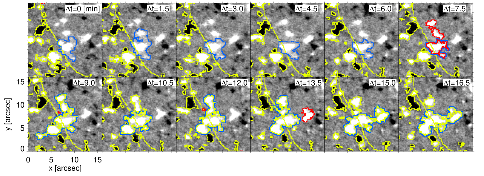
Figure 2.— Example of merging events. An IN element detected by YAFTA as a single feature (blue contours) merges with a NE patch at $\Delta t=9.0$ min and becomes a NE feature itself. NE elements are indicated with yellow contours. This specific IN patch undergoes several mergings with other IN patches during the sequence, revealing the full complexity of interactions between magnetic flux concentrations. For example, two smaller IN features to the North merge with it at $\Delta t=9.0$ min. The same happens with another IN element to the West at $\Delta t=15.0$ min. The red contours mark the boundaries of the IN patch right before merging with the NE, as well as the boundaries of the other IN elements that will become part of it. The flux they enclose is taken to be the contribution to the NE of all the IN patches participating in the process. Note that the small IN elements that merge with the main IN feature at 9 min are assimilated into it. Therefore, we mark them as NE patches from that moment on and do not change their character when they separate from their parent at 10.5 and 15.0 min.

3.3. Identification of IN and NE elements

Magnetic features that appear in the interior of supergranular cells (i.e., inside the boundaries defined above) are taken to be IN elements. Elements born by fragmentation of an IN element are also classified as IN patches. IN elements keep their character unless they merge with NE features, in which case they become part of the NE and are tagged accordingly.

The identification of NE patches is more involved. In the first frame, elements that have their flux-weighted centers (FWC) inside of a NE region are considered to be NE features. Also, only in the first frame, elements that are touching a NE region are counted as NE elements because we do not know their history.

For all $i>1$ frames, magnetic features are marked as NE elements if they overlap more than 70$\%$ with NE structures from the previous $i-1$ frame or if their FWCs are located inside any of the NE patches detected in the $i-1$ frame.

When an element appears by fragmentation, it is considered to belong to the NE if its parent is already marked as a NE structure. At any time, an element that appears in situ inside the NE is considered to be part of the NE.

3.4. Calculation of the IN contribution to the NE flux

Merging and cancellation are the only two processes through which IN elements can modify the flux of the NE. These processes involve a direct interaction between IN and NE elements. IN features that merge with NE patches add flux to the NE, while those canceling with opposite-polarity elements remove flux from the NE. Their respective contributions are determined as follows.

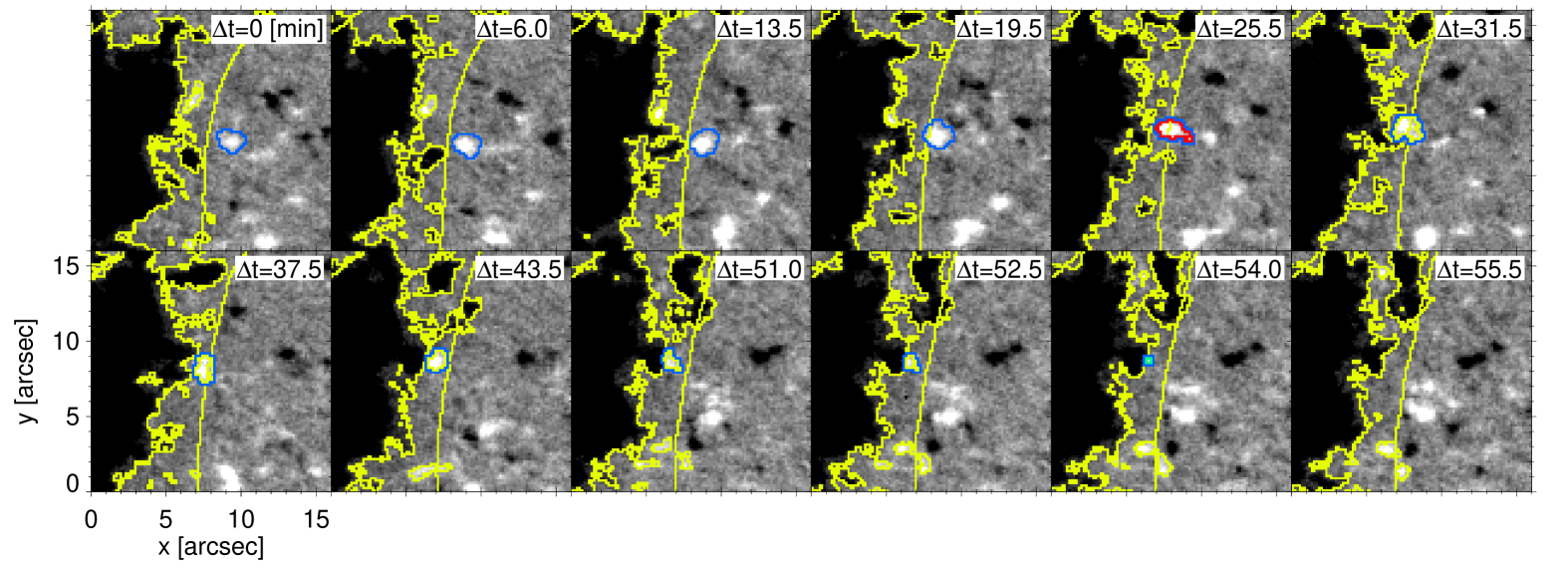
Figure 3.— Example of an IN element (blue contours) canceling with NE patches (yellow contours). The contours are those provided by YAFTA, except that the blue ones have been expanded by 1 pixel for visualization purposes. The red contours mark the flux used to compute the contribution of the IN element to the NE. The green contour at $\Delta t=54$ min outlines the canceling IN element in the last frame where it is visible.

3.4.1 Contribution through merging events

When an IN element merges with a NE patch, the flux it contributes to the NE is calculated in the frame where it is visible as an individual feature for the last time. We consider only the pixels of the IN element that do not overlap with any of the NE patches of the previous frame, to avoid including NE flux due to fragments that YAFTA may have erroneously added to the IN feature.

A detection problem arises when IN flux from the previous frame converts into NE flux in the current frame, without ever being recognized by YAFTA as a unique magnetic element. This happens when some portion of an IN element fragments from its parent and merges with a NE patch between two consecutive frames. To find and count such events, we calculate the difference between logical masks of NE elements in frame $i$ and frame $i-1$. All pixels different from zero in the difference mask are assigned the flux densities they had in frame $i$. On such “partial” magnetogram we apply the downhill method. This method finds all contiguous like-polarity pixels above a given threshold that lie on the same flux peak (Welsch & Longcope, 2003). Every flux structure larger than 16 pixels exceeding a signal threshold of 3$\sigma$ is taken to be a magnetic element. Finally, we dilate these features to the nearest neighboring pixel. If they overlap the NE mask from the current frame and their FWCs are not located inside of the NE region, they are counted as contributing IN fragments that were not detected by the code.

A similar situation occurs when an IN element merges with a NE fragment which is not detected by YAFTA as an individual feature because the fragmentation and the merging take place in the same frame. For YAFTA, the IN element continues to be an IN element of increased flux and size. If the NE fragment had more flux than the IN patch, however, their common FWC will more likely be located inside the NE feature of the previous frame from which the fragment detached, and our method will recognize the entire element as a NE patch. To evaluate the IN contribution in this case, and reject the NE portion of the flux, we apply the downhill method described above.

A complex example of an IN element merging with NE patches is shown in Figure 2. This element interacts with other IN features during the sequence (e.g., at $\Delta t=9.0$ and 15.0 min). The red contours indicate the flux contributed to the NE by each of the IN elements.

3.4.2 Contribution through cancellation events

Cancellation events are found by searching for all closely located, opposite-polarity elements that disappear in the current frame. More precisely, we take an IN element at the moment of disappearance, dilate its border by 2 pixels and, if it overlaps a NE patch of opposite polarity, count the IN element as a canceling flux feature. To determine how much flux it removes from the NE, we go back in time and take the total flux of the IN element at the moment when the cancellation started (i.e, when the IN patch touched the opposite-polarity NE element for the first time). This flux is corrected for all the changes caused by the merging and fragmentation processes that might happen during the cancellation event.

The same procedure is repeated for NE elements that disappear by cancellation with IN elements. The latter may survive the process, but they remove flux from the NE. Their contribution is taken to be the flux of the NE patch at the beginning of the cancellation.

In Fig. 3 we show an example of an IN feature canceling with NE patches and how the interaction is interpreted.

3.4.3 Practical implementation and limitations

The identification of IN elements merging or canceling with NE features is carried out in the following way. In frame $i$ we examine all the NE and IN elements that lose their labels and disappear as individual entities. We check whether they merged or canceled with another element. Only if the interaction involves an IN element and a NE patch do we count the former as contributing to the NE. In the case of mergings, the flux carried by the IN patch in frame $i-1$ is assumed to be transferred to the NE in frame $i$. In the case of cancellations, the initial flux of the element that disappears completely is taken to be the contribution of the IN to the NE in frame $i$.

This method covers the situation in which IN elements merge with weak NE fragments. Being dominant in flux they keep their labels, but they must be considered part of the NE from that moment on (as well as their children in case of fragmentation). Therefore, we tag them as NE patches, except when they are inside the IN. This is done for computational convenience—otherwise they would quickly turn all IN patches into NE features through mergings with other elements inside the supergranular cell. IN features not tagged as NE patches are considered to contribute to the NE if they enter a NE region or end their lives interacting with a NE patch.

The procedure just described determines the flux transferred to the NE taking into account only the first interaction. IN elements that cancel completely remove flux from the NE and cannot undergo further interactions, so their contribution is estimated correctly. However, in the case of mergings our calculations provide only an upper limit. The reason is that an IN element may first merge with a NE patch and later cancel with another NE patch, so that part of it would actually remove rather than add flux to the NE. Unfortunately, once the element loses its identity because of the merging there is no way to know whether this occurs at all.

Table 2Magnetic elements detected by YAFTA

	Data set 1	Data set 2
Total number of elements	265 933	316 097
IN regions
Total IN elements	160 859	215 775
Positive IN elements	80 293	108 902
Negative IN elements	80 566	106 873
Mean effective size	$1\farcs 0$	$1\farcs 0$
Mean absolute flux $[\times 10^{16}\mbox{~{}Mx}]$	12.7	13.6
Mean flux $[\times 10^{16}\mbox{~{}Mx}]$	$-1.1$	$-0.08$
NE regions
Total NE elements	105 074	100 322
Positive NE elements	50 777	43 065
Negative NE elements	54 297	57 257
Mean effective size	$1\farcs 8$	$2\farcs 0$
Mean absolute flux $[\times 10^{16}\mbox{~{}Mx}]$	71.7	123.3
Mean flux $[\times 10^{16}\mbox{~{}Mx}]$	$-7.6$	$-78.6$

4. Results

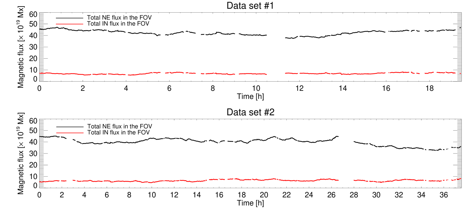
Figure 4.— Temporal evolution of the total flux of NE and IN regions (black and red curves) in data sets 1 and 2.

Using YAFTA, we followed the evolution of the magnetic flux patches visible in the entire FOV. In total we detected 265 933 elements in data set 1 and 316 097 in data set 2. Table 2 provides detailed information broken down into NE and IN regions. IN patches are noticeably more abundant than NE patches, accounting for more than 60% of all the elements. Such a result is expected from their larger appearance rates and shorter lifetimes. In the data sets used here, IN elements have a mean absolute flux of about $13\times 10^{16}$ Mx. Their mean flux is less than approximately $10^{16}$ Mx, indicating that the two polarities are nearly balanced. By contrast, NE elements are much stronger, with mean absolute fluxes of $72\times 10^{16}$ Mx in data set 1 and $123\times 10^{16}$ Mx in data set 2. Both time sequences exhibit a pronounced NE flux imbalance that may reach up to $-79\times 10^{16}$ Mx.

The figures in Table 2 do not reflect the number of unique elements in the magnetograms because many of them are counted multiple times by YAFTA. Our analysis is not affected by this behavior because we are interested only in IN features interacting with NE elements. If they survive the interaction, we label them as NE elements to avoid their contributing more than once to the NE flux.

4.1. Temporal evolution of IN and NE fluxes

Figure 4 shows the temporal evolution of the total NE and IN fluxes for the two data sets analyzed here. These values have been calculated adding the absolute fluxes of all the detected NE and IN magnetic elements, respectively. Gaps in the curves are the result of transmission problems and data recorder overflows. Other short interruptions coincide with magnetograms that contain recovered stripes.

Both the NE and IN fluxes remain stable over time, showing only small fluctuations (less than 8% and 12% rms, respectively). This indicates that the NE and IN have reached a steady state. Individual supergranular cells are appearing, evolving, and disappearing in the time sequences, but the FOV is sufficiently large as for the results not to depend on the variations of single cells.

The total NE and IN fluxes in data set 1 are on average $42.5\times 10^{19}$ Mx and $6.9\times 10^{19}$ Mx, respectively. For data set 2, the corresponding values are $39.8\times 10^{19}$ Mx and $6.5\times 10^{19}$ Mx. Thus, 14% of the total QS (NE$+$IN) flux is in the form of IN elements. The remainder is provided by the NE, with a total flux of $5.5-8.0\times 10^{23}$ Mx over the entire Sun. The minimum and maximum contributions of the IN to the QS flux observed in our data sets are 10% and 20%, respectively.

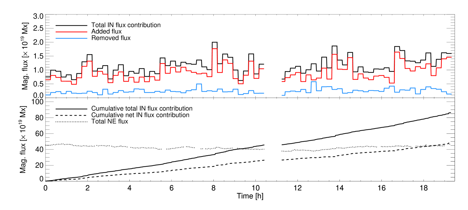
Figure 5.— Contribution of the IN to the NE in the full FOV of data set 1. We use 15 minute bins to represent the data. Top panel: total contribution (black), defined as the sum of the absolute flux that the IN adds to the NE through mergings (red) and the absolute flux that the IN removes from the NE through cancellations (blue). The average total contribution per 15 min bin is $1.15\times 10^{19}$ Mx, the average added flux is $0.91\times 10^{19}$ Mx, and the average removed flux is $0.24\times 10^{19}$ Mx. Bottom panel: Cumulative contribution of the IN to the NE flux. The solid line represents the total IN flux transferred to the NE (added plus removed absolute flux), while the dashed line gives the net contribution of the IN to the NE (added minus removed flux). The total NE flux in the entire FOV is indicated by the dotted line.

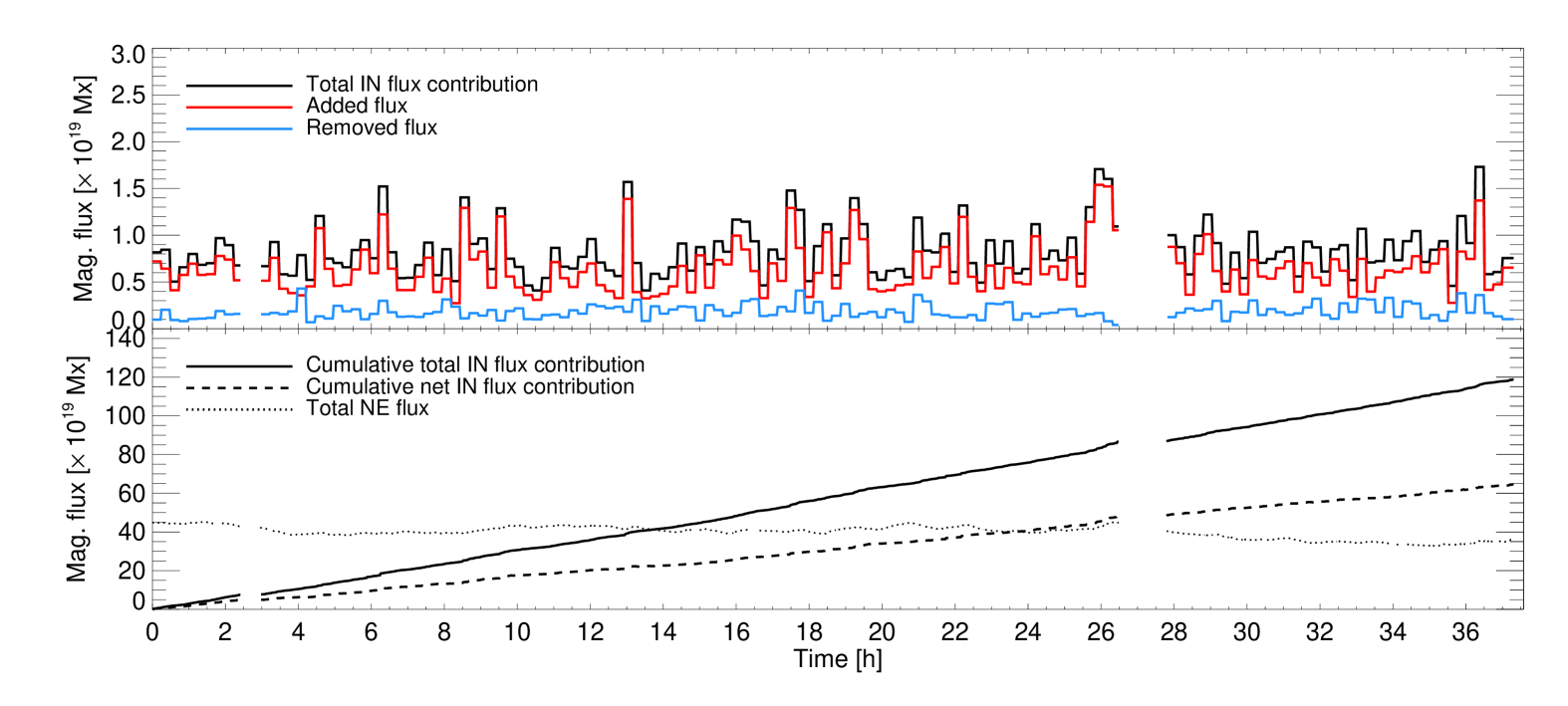
Figure 6.— Same as Figure 5, but for data set 2. The average total IN contribution per 15 min bin is $0.82\times 10^{19}$ Mx, the average added flux is $0.64\times 10^{19}$ Mx, and the average removed flux is $0.18\times 10^{19}$ Mx.

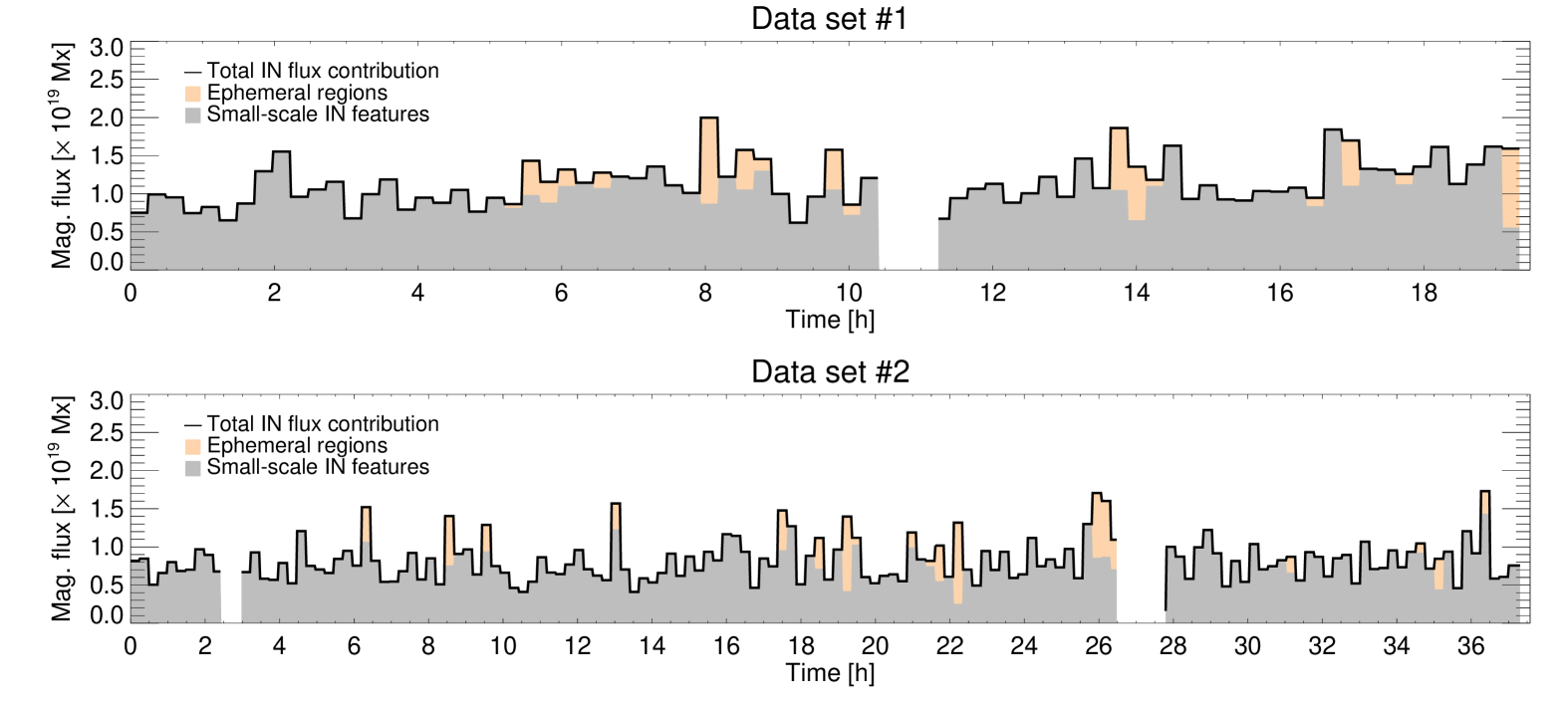
Figure 7.— IN contribution to the NE flux in the form of isolated IN elements (gray shaded areas) and ER patches (orange shaded areas). The total IN contribution is represented by the black curves.

4.2. Contribution of the IN to the NE flux

The top panel of Figure 5 shows how much flux the IN transfers to the NE as a function of time in data set 1. The two possible contributions are separated, namely flux added to the NE through mergings (red curve) and flux removed from the NE through cancellations (blue curve). Their sum is indicated by the black curve. The data have been binned over 15 minutes. Each bin represents the IN flux contributed to the NE during that period of time.

As can be seen, the total IN contribution to the NE shows some variations over the 19.5 h of observation, but it is relatively constant at about $4.6\times 10^{19}$ Mx h^-1 in the full FOV, or $1.4\times 10^{24}$ Mx day^-1 over the entire solar surface. Clearly, the IN is more efficient in injecting flux than in removing it. Merging of like-polarity patches is the dominant process and involves 3.8 times more flux than cancellations.

In the bottom panel of Figure 5 we show the cumulative IN contribution to the NE considering all the flux deposited in the NE (solid line) and the net flux gained by the NE (dashed line). The former is the total IN flux that actually interacts with NE patches, independently of the final outcome of the interaction. The latter is the net flux added to the NE (mergings minus cancellations).

The slope of the two curves does not change with time, indicating that the IN supplies flux to the NE at a nearly constant rate. Very interestingly, in only $\sim$9.5 hours the NE receives from the IN as much flux as it contains. Most—but not all—of that flux is incorporated into the NE. Considering only the net flux that remains in the NE (dashed line), the IN needs some 18 h to supply as much flux as is present in the NE at any one time.

The IN contribution to the NE flux in data set 2 is shown in Figure 6. Just like in the first data set, mergings dominate over cancellations by a factor of 3.6, the result being that the IN adds flux to the NE continually (top panel). On average, the IN contributes a total of $3.3\times 10^{19}$ Mx h^-1 to the NE in the observed FOV, or $1.6\times 10^{24}$ Mx day^-1 over the entire solar surface. The cumulative contributions are shown in the bottom panel, both for the total flux transferred to the NE (solid line) and for the net flux which is actually incorporated into the NE (dashed line). The dotted line represents the total NE flux in the FOV. According to these curves, the IN transfers as much flux as the NE contains in 13.5 h, or in some 24 h considering only the net contribution to the NE.

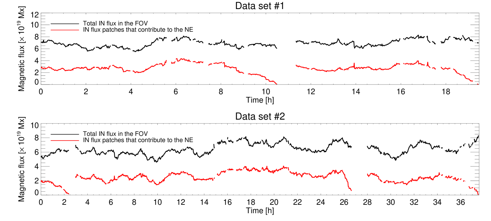
Figure 8.— Fraction of the total IN magnetic flux that converts into NE flux, for data sets 1 and 2 (top and bottom, respectively). The red curves show the instantaneous flux carried by the IN patches that will convert to the NE at any later time. For reference, the black curves represent the IN flux in the entire FOV.

Thus, the IN continually supplies flux to the NE. Since the total NE flux does not change with time, flux must be removed from the NE at a similar rate through cancellations and in-situ disappearances. However, a detailed analysis of such processes is beyond the scope of this paper, as it would require careful interpretation of the YAFTA results in the extremely crowded and dynamic regions of the NE. First attempts to quantify the interactions between magnetic elements in the NE have been presented by Iida et al. (2012).

4.3. Contribution of ERs to the NE flux

The current paradigm is that ERs provide the flux needed to maintain the network. Our very long magnetogram sequences can be used to determine the percentage of the IN flux transferred to the NE that is due to ERs. Detecting ERs in the Hinode magnetograms is difficult because YAFTA does not recognize the presence of large-scale structures. To circumvent this problem, we manually identified ERs as clusters of mixed-polarity flux patches appearing together and separating from each other with time. To qualify as an ER, at least one element in the cluster had to reach a flux content of $3\times 10^{18}$ Mx, the threshold set by Hagenaar et al. (2003). The individual ER patches were then tracked and counted as contributing to the NE if they had interactions with NE patches. We detected five ERs in data set 1 and nine in data set 2, roughly consistent with the appearance rate of 430 per hour estimated by Chae et al. (2001) over the entire solar surface.

The black curves in Figure 7 show the total IN contribution to the NE already displayed in the top panels of Figures 5 and 6. For each 15 minute bin we separate the flux transferred to the NE by isolated IN patches (gray shaded areas) and ER patches (orange shaded areas).

As can be seen, ERs play only a minor role in the flux transfer from the IN to the NE. They inject about $1.1\times 10^{23}$ Mx day^-1 into the IN, but this is less than $\sim$8% of the total IN flux that reaches the NE in the two data sets. Thus, despite the large amount of flux they carry, ERs are not the main contributors to the NE flux. More than 90% of the flux comes from weak, isolated IN patches.

4.4. Fraction of total IN flux transferred to the NE

After appearing in the interior of supergranular cells, IN elements migrate toward the cell boundaries where the NE resides. However, not all IN elements end up in the NE, since many of them disappear in situ or cancel with other IN elements before reaching the NE. Here we study what fraction of the IN flux actually makes it to the NE.

The black curves in Figure 8 show the temporal evolution of the IN flux in the entire FOV of data sets 1 and 2. The total flux carried by the IN patches that interact with the NE at any later time is indicated with the red curves. For this calculation we take into account all fragmentations and partial cancellations that the elements may undergo before interacting with the NE. Close to the end of each continuous observing periods there are artificial drops of the IN flux contributing to the NE. They reflect the lack of information about the evolution of IN elements during the data gaps. Some of the elements may interact with the NE, but they are not counted because it is not possible to identify them, producing drops in the curves.

On average, we find that 38% of the IN flux generated in the interior of supergranules eventually contribute to the NE. Both data sets show very similar percentages. The rest of elements disappear inside the IN by cancellations or in-situ fading and never reach the NE (see Paper II of this series by Gošić & Bellot Rubio, in preparation). Thus, a significant fraction of the observed IN flux is incorporated into the NE, emphasizing the importance of the IN for the maintenance—and arguably also the existence—of the magnetic NE.

5. Discussion and Conclusions

We have analyzed magnetic flux elements in NE and IN regions using long-duration, high-resolution Hinode/NFI magnetogram sequences. We carefully processed the data to facilitate the tracking of magnetic features and the identification of patches after interactions. These measurements give us the opportunity to study for the first time the evolution of QS magnetic fields in the range $10^{16}-10^{20}$ Mx on scales from minute to days. After identifying NE and IN flux concentrations, we followed them with an automatic tracking algorithm to examine how the IN contributes flux to the NE. We calculated the transfer of IN flux to the NE in a direct way, using the instantaneous flux of the IN elements that interact with NE patches.

In our observations, the total IN and NE fluxes are very stable and exhibit only small variations with time. IN regions are in nearly perfect polarity balance. By contrast, NE regions show clear polarity imbalances in both data sets. On average, 14% of the QS flux is in the form of IN elements. This value is consistent with the estimates of Wang et al. (1995). The instantaneous ratio, however, varies in the range from 10% up to 20%. Our definition of NE and IN elements is based on spatial location—derived from horizontal flow maps—rather than on flux densities or sizes. This may have resulted in lower percentages because some small-scale IN elements were probably labeled as NE features. If flux density or size criteria had been used instead, those elements would have more likely been recognized as IN elements. However, as they appear close to NE patches in supergranular downflows, it seems reasonable to mark them as NE fragments.

We have shown that IN elements continuously supply flux to the NE, confirming the prediction by Lamb et al. (2008) that it should be possible to observe interactions between NE and IN elements on spatial scales not accessible to MDI.

We estimate that up to 38% of the magnetic flux appearing inside supergranular cells moves toward the edges of supergranules and interact with the NE. IN features merge or cancel with preexisting NE patches, adding or removing flux from the NE. The first process is dominant, by a factor of 3.6–3.8. The IN contributes a total flux of $\sim 1.5\times 10^{24}$ Mx day^-1 to the NE. Thus, IN regions can generate and transfer as much magnetic flux as is present in NE regions in only 9–13 h. Taking into account that not all elements add flux to the NE, the time needed by the IN to supply a net flux equal to that present in the NE is 18-24 hours.

Our estimates of the IN contribution to the NE flux are more accurate than those based on flux emergence or disappearance rates. This is because we directly measure how much flux converts into NE flux or cancels with NE elements instantaneously, whereas flux emergence and cancellation rates include a fraction of elements that never interact with the NE and therefore should not be counted. In our data sets, the temporal scales on which the IN could supply as much flux as is contained in the NE are shorter than the 36–72 h reported by Schrijver et al. (1997), but also significantly longer than the lower limit of 1 h found by Hagenaar et al. (2008). Both analyses used SOHO/MDI data, and therefore could not see most of the IN flux.

Our observations made it possible to determine in a direct way the actual contribution of ERs to the NE flux. To estimate the flux they transfer to the NE we have considered as ERs all the clusters of mixed-polarity patches emerging in the same area with at least one of the patches reaching $3\times 10^{18}$ Mx. During the approximately 58 hours of monitoring of the quiet Sun performed with the Hinode NFI we see 14 ERs. We find that ERs transfer flux to the network at a rate of $1.1\times 10^{23}$ Mx day^-1, which is only slightly larger than the ER emergence rate of $7.2\times 10^{22}$ Mx day^-1 reported by Schrijver et al. (1997) but less than 8% of the total IN contribution to the NE found here. This entails a change of paradigm, as most of the IN flux transferred to the NE seems to come from weak, isolated IN elements and not from ERs.

The main result of this work is that NE regions receive a substantial and constant flux inflow from the solar IN. Actually, small-scale IN elements appear to be the main and most permanent source of flux for the NE. Their origin however remains poorly understood. To shed light on this issue, we will determine the flux appearance and disappearance rates in the IN in Paper II of this series, while Paper III will be devoted to study the modes of appearance of IN elements on the solar surface.

References

- Brault & Neckel (1987) Brault, J. W., & Neckel, H. 1987, Spectral Atlas of Solar Absolute Disk-averaged and Disk-Center Intensity from 3290 to 12510 Å, ftp://ftp.hs.uni-hamburg.de/pub/outgoing/FTS-Atlas
- Bellot Rubio & Orozco Suárez (2014) Bellot Rubio, L.R., & Orozco Suárez, D. 2014, Living Reviews in Solar Physics, submitted
- Centeno et al. (2007) Centeno, R., Socas-Navarro, H., & Lites, B. et al. 2007, ApJ, 666, L137
- Chae et al. (2001) Chae, J., Martin, S. F., & Yun, H. S. et al. 2001, ApJ, 548, 497
- DeForest et al. (2007) DeForest, C. E., Hagenaar, H. J., & Lamb, D. A. et al. 2007, ApJ, 666, 576
- De Wijn et al. (2009) De Wijn, A. G., Stenflo, J. O., & Solanki, S. K. et al. 2009, Space Sci. Rev., 144, 275
- Gošić (2012) Gošić, M. 2012, Master Thesis, University of Granada (Spain)
- Hagenaar (2001) Hagenaar, H. J. 2001, ApJ, 555, 448
- Hagenaar et al. (2008) Hagenaar, H. J., DeRosa, M. L., & Schrijver, C. J. 2008, ApJ, 678, 541
- Hagenaar et al. (2003) Hagenaar, H. J., Schrijver, C. J., & Title, A. M. 2003, ApJ, 584, 1107
- Harvey & Martin (1973) Harvey, K. L., & Martin, S. F. 1973, Sol. Phys., 32, 389
- Harvey et al. (1975) Harvey, K. L., Harvey, J. W., & Martin, S. F. 1975, Sol. Phys., 40, 87
- Iida et al. (2012) Iida, Y., Hagenaar, H. J., & Yokoyama, T. 2012, ApJ, 752, 149
- Kosugi et al. (2007) Kosugi, T., Matsuzaki, K., Sakao, T., et al. 2007, Sol. Phys., 243, 3
- Lamb et al. (2008) Lamb, D. A., DeForest, C. E., & Hagenaar, H., J. et al. 2008, ApJ, 674, 520
- Lamb et al. (2010) Lamb, D. A., DeForest, C. E., & Hagenaar, H., J. et al. 2010, ApJ, 720, 1405
- Lites (2002) Lites, B. W. 2002, ApJ, 573, 431
- Livingston & Harvey (1975) Livingston, W. C., & Harvey, J. 1975, BAAS, 7, 346
- Martin (1990) Martin, S. F. 1990, IAUS, 138, 129
- Martínez González & Bellot Rubio (2009) Martínez González, M. J., & Bellot Rubio, L. R. 2009, ApJ, 700, 1391
- Meunier et al. (1998) Meunier, N., Solanki, S. K., & Livingston, W. C. 1998, A&A, 331, 771
- November & Simon (1988) November, N., & Simon, W. G. 1998, ApJ, 333, 427
- Orozco Suárez et al. (2008) Orozco Suárez, D., Bellot Rubio, L. R., & del Toro Iniesta, J. C. et al. 2008, ApJ, 481, L33
- Orozco Suárez et al. (2012) Orozco Suárez, D., Katsukawa, Y., & Bellot Rubio, L. R. 2012, ApJ, 758, L38
- Parnell et al. (2009) Parnell, C. E., DeForest, C. E., & Hagenaar, H. J. et al. 2009, ApJ, 698, 75
- Sánchez Almeida & Martínez González (2011) Sánchez Almeida, J., & Martínez González, M. 2011, ASP Conf. Series, 437, 451
- Scherrer et al. (1995) Scherrer, P. H., Bogart, R. S., & Bush, R. I. et al. 1995, Sol. Phys., 162, 129
- Schrijver & Harvey (1994) Schrijver, C. J., & Harvey, K. L. 1994, Sol. Phys., 150, 1
- Schrijver et al. (1997) Schrijver, C. J., Title, A. M., & Hagenaar, H. J. et al. 1997, ApJ, 487, 424
- Simon et al. (2001) Simon, G. W., Title, A. M., & Weiss, N. O. 2001, ApJ, 561, 427
- Solanki (1993) Solanki, S. K. 1993, Space Sci. Rev., 63, 1
- Straus et al. (1992) Straus, T., Deubner, F.-L., & Fleck, B. 1992, A&A, 256, 652
- Title (2000) Title, A. M. 2000, Philos. Trans. Roy. Soc. London A, 358, 657
- Title et al. (1989) Title, A. M., Tarbell, T. D., Topka, K. P., et al. 1989, ApJ, 336, 475
- Thornton & Parnell (2010) Thornton, L. M., & Parnell, C. E. 2010, Sol. Phys., 269, 13
- Tsuneta et al. (2008) Tsuneta, S., Ichimoto, K., & Katsukawa, Y. 2008, Sol. Phys., 249, 167
- Wang & Zirin (1987) Wang, H., & Zirin, H. et al. 1987, Sol. Phys., 115, 205
- Wang et al. (1995) Wang, J., Wang, H., & Tang, F. et al. 1995, Sol. Phys., 160, 277
- Wang et al. (2012) Wang, J., Zhou, G., Jin, C., & Li, H. 2012, Sol. Phys., 278, 299
- Welsch & Longcope (2003) Welsch, B. T., & Longcope, D. W. 2003, ApJ, 588, 620
- Zhou et al. (2010) Zhou, G., Wang, J., & Jin, C. 2010, Sol. Phys., 267, 63z
- Zhou et al. (2013) Zhou, G., Wang, J., & Jin, C. 2013, Sol. Phys., 283, 273
- Zirin (1985) Zirin, H. 1985, AuJPh, 38, 961
- Zirin (1987) Zirin, H. 1987, Sol. Phys., 110, 101