Agent based models for wealth distribution with preference in interaction

Abstract

We propose a set of conservative models in which agents exchange wealth with a preference in the choice of interacting agents in different ways. The common feature in all the models is that the temporary values of financial status of agents is a deciding factor for interaction. Other factors which may play important role are past interactions and wealth possessed by individuals. Wealth distribution, network properties and activity are the main quantities which have been studied. Evidence of phase transitions and other interesting features are presented. The results show that certain observations of real economic system can be reproduced by the models.

I Introduction

One of the main objectives of several models in econophysics is to reproduce the Pareto tail or power-law tail in the wealth/income distribution in several economy Pareto:1897 . According to Pareto law, the probability that the income/wealth of an agent is equal to $m$ is given by,

$$P(m)\sim m^{-(1+\nu)},$$ (1)

where $\nu$ is called the Pareto exponent. The value of the exponent usually varies between $1$ and $3$ Mandelbrot:1960 ; EIWD ; EWD05 ; ESTP ; SCCC ; Yakovenko:RMP ; datapap .

Some of the models proposed to yield the above distribution are inspired by the kinetic theory of gases which derives the average macroscopic behaviour from the microscopic interactions between molecules. Agents can be regarded as molecules and a trading process can be regarded as an interaction between them. In a typical trading a pair of traders exchange wealth, respecting local conservation of wealth in any trading marjitIspolatov ; Dragulescu:2000 ; Chakraborti:2000 ; Chatterjee:rev ; Chakrabarti:2010 ; Chatterjee:2010 , similar to an elastic collision between molecules. Consequently, the total wealth remains conserved. These agent based models have a microcanonical description and nobody ends up with negative wealth (i.e., debt is not allowed). Thus, for two agents $i$ and $j$ with money $m_{i}(t)$ and $m_{j}(t)$ at time $t$, the general trading process is given by:

$$m_{i}(t+1)=m_{i}(t)+\Delta m;\ m_{j}(t+1)=m_{j}(t)-\Delta m;$$ (2)

time $t$ changes by one unit after each trading. The advantage of such models is that here dynamics at individual level can be studied. In a simple conservative model proposed by Dragulescu and Yakovenko (DY model) Dragulescu:2000 , $N$ agents exchange wealth or money randomly keeping the total wealth $M$ constant. The steady-state ($t\rightarrow\infty$) wealth therefore follows a Boltzmann-Gibbs distribution: $P(m)=(1/T)\exp(-m/T)$; $T=M/N$, a result which is robust and independent of the topology of the (undirected) exchange space Chatterjee:rev .

An additional concept of saving propensity was introduced first by Chakraborti and Chakrabarti Chakraborti:2000 (CC model hereafter). Here, the agents save a fixed fraction $\lambda$ of their wealth when interacting with another agent. This results in completely different types of wealth distribution curves, very close to Gamma distributions Patriarca:2004 ; Repetowicz:2005 ; Lallouache:2010 which fit well to empirical data for low and middle wealth regime datapap . The model features are basically similar to Angle’s work Angle . In a later model proposed by Chatterjee et. al. Chatterjee:2004 (CCM model hereafter) it was assumed that the saving propensity has a distribution, i.e., $\lambda$’s are now agent dependent and this immediately led to a wealth distribution curve with a Pareto-like tail. Apart from these gas-like models, there are several other models of the wealth distribution. Some of these models depend on stochastic process Garl ; Sornette which cannot be realized as a real trading process. Another model is the Lotka-Volterra model where wealth of an agent at a particular step depends on their wealth in the previous step as well as the average wealth of all agents Solomon ; Malcai . The main problem in all these models is that here wealth exchange between agents is not allowed and therefore leads to a situation far from reality.

Although wealth distribution is one of the most important feature for which the models had been proposed, there are other interesting characteristics of the market which a model should be able to reproduce. Financial institutions are seen to exhibit some interdependence and links are formed among them depending on several economic factors leading to network structure. In Allen ; Babus the problem of network formation in a financial system have been addressed. One can then study the network like features, e.g., the kind of clusters which are formed among agents and the behaviour of the degree distribution for better explanation of several economic phenomena. Some real data are available to this respect. It has been shown that within a small interval of time most clusters are of size 2 tummi ; tummi2 which can be termed as ‘dimerisation’. Another observation is regarding the activity, i.e., the distribution of the volume of individual trade that also follows a power law with an exponent $\simeq 4.3$ Gabaix . These features suggest that one needs to introduce some preference in the interaction between agents.

In almost all the wealth exchange models, the interacting agents are selected randomly and any two agents have equal probability to interact. In this paper, we incorporate preferential attachement to agents for interaction as well as in the choice of agents in some cases. Such preferences need not be limited to geographically nearby neighbours. In manna1 , a preference in the selection of agents (according to their wealth) had been considered, however, the interacting agents were uncorrelated otherwise.

To obtain an optimized kinetic exchange model for trade, several features have to be incorporated. Our basic assumption is that two agents will interact only when their wealths are “close”. So in the simplest model, only such a feature is incorporated in an otherwise DY like model. More features have been added to obtain results closer to reality. In all the models wealth distribution, network features and other properties are studied.

II Quantities Calculated

We consider kinetic exchange type models where the interactions are of DY type. The simulation is done for a maximum of $N=1024$ agents. Initially the total money $M$ is distributed among the agents randomly. The stationary state is obtained after a typical relaxation time by checking the stability of the wealth distribution in the successive Monte Carlo (MC) steps, where one MC step is equivalent to $N$ pairwise interactions. The wealth distribution is obtained by averaging over a finite but large number of time steps. Finally the configurational averaging is done over a number of realizations to obtain the wealth distribution.

Results for the following features have been presented in the paper:

1. Wealth Distribution: $P(m)$ (already introduced in sec I),

2. Degree Distribution: The number of agents with whom one particular agent interacts within one MC time step, averaged over all time step is the degree of an agent. $D(k)$ denotes the probability that an agent has degree $k$.

3. Activity Distribution: Activity distribution is defined as the number of transactions made by one individual in one MC timestep, averaged over all timesteps. We use $Q(A)$ to denote the activity distribution.

4. Average degree with wealth $m$: $d(m)$, the average degree of an agent with money $m$ is also calculated to investigate whether the degree is correlated to wealth.

In all the cases, we have taken $M=\sum_{i=1}^{N}m_{i}$ to be equal to $N$.

III Models and Results

III.1 Model A

In model A, the only criteria that an interaction between two agents will take place is that they should be financially close. The probability of interaction between agents $i$ and $j$ is taken as

$$P_{ij}\propto|m_{i}-m_{j}|^{-\alpha}.~{}~{}~{}~{}~{}\alpha>0.$$ (3)

Note that, it may happen that wealth of two agents $i$ and $j$ are equal, i.e., $m_{i}=m_{j}$. In that case, it was considered that interaction between $i$ and $j$ would occur as a sure event. However as $m$ is continuously varying such cases are extremely rare.

Wealth distribution for model A for extreme values of $\alpha$ are as follows :

1. For $\alpha=0$, we get back the DY model.

2. When $\alpha>>1$, the tail of the wealth distribution has a power law form.

The wealth distribution for different values of $\alpha$ are shown in Fig. 1.

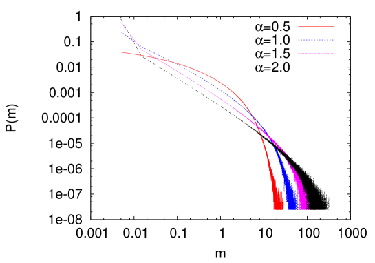
Figure 1: (Color online) Plot of $P(m)$ as a function of $m$ for model A with $N=1024$. Total money $M=N$.

It is seen from the figure that the plots have the general form $am^{-b}\exp(-cm)$. The variations of $b$ and $c$ with $\alpha$ are shown in Fig. 2 and those with $N$ are shown in the inset.

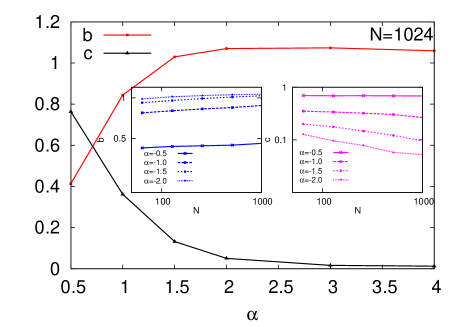
Figure 2: (Color online) Variation of $b$ and $c$ with $\alpha$ for model A for N=1024. Inset shows (left) variation of $b$ with $N$ for model A and (right) variation of $b$ with $N$ for model A.

Variation of $c$ with $N$ indicates that it vanishes at large values of $\alpha$ in the thermodynamic limit. The value of $b$ increases with increasing $\alpha$ and $N$. For $\alpha\gtrsim 2$ it is close to $1$. One can safely conclude that for $\alpha>2$, the exponential cut-off vanishes. However, the corresponding Pareto exponent is rather small ($\nu=b-1\sim 0.1$).

Degree distribution $D(k)$ for model A has an exponential form and does not change appreciably with $\alpha$ as is shown in the left panel of Fig. 3.

In the right panel of Fig. 3 the activity distribution $Q(A)$ for model A is shown. It has an exponential form that does not change with $\alpha$.

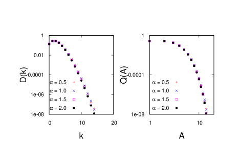
Figure 3: (Color online) Plot of D(k) and Q(A) for model A with $N=1024$.

Average degree of an agent with wealth $m$ is represented by $d(m)$ and is shown in Fig. 4.

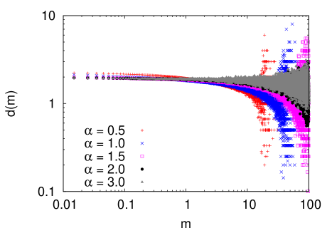
Figure 4: (Color online) Plot of $d(m)$ as a function of $m$ for model A.

It is seen that $d(m)$ is independent of the wealth possessed by an individual; more so for larger values of $\alpha$. However, for large values of $m$ ($m>10$), there is appreciable fluctuation.

III.2 Model B

In model B, in addition to the assumption that transactions are more probable for agents who are financially close to each other, it is assumed that probability of transaction increases with past number of interactions. Probability of interaction between $i$ and $j$ taken in model B is,

$$P_{ij}\propto|m_{i}-m_{j}|^{-\alpha}(c_{ij}+1)^{\gamma},$$ (4)

where $c_{ij}$ is the number of interactions which have taken place already between $i$ and $j$. The factor $1$ is added to $c_{ij}$ to ensure that two persons who have not traded with each other yet can still interact.

The wealth distributions for two different values of $\alpha$ for various values of $\gamma$ are shown in Fig. 5.

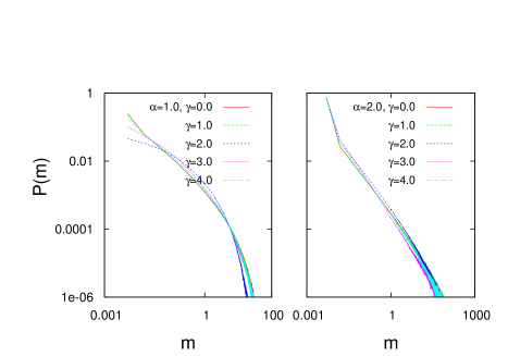
Figure 5: (Color online) Plot of $P(m)$ as a function of $m$ for model B with parameters $\alpha=1.0$ and $2.0$, $\gamma=0.0,1.0,2.0,3.0$ and $N=1024$.

For $\alpha\geq 2$ one gets the power law tail but the corresponding values of $\nu$ are still quite small ($\mathcal{O}(0.1))$. Some of the values of $\nu$ obtained for different chosen sets of parameters for model B are shown in Table 1.

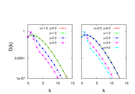
Figure 6: (Color online) Plot of degree distribution $D(k)$ as a function of degree $k$ for model B with parameters $\alpha=1.0$ and $2.0$, $\gamma=0.0,1.0,2.0,3.0$ and $N=1024$.

The degree distribution is shown in Fig. 6. The mean degree decreases for higher values of $\gamma$. The mean degree $\langle k\rangle$ and fluctuation $\frac{\Delta k}{\langle k\rangle}$ are plotted against $\gamma$ (Fig. 7).

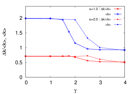
Figure 7: (Color online) Plot of mean degree $\langle k\rangle$ and fluctuation $\frac{\Delta k}{\langle k\rangle}$.

It shows an interesting feature: $\langle k\rangle$ has a value equal to $2$ for small $\gamma$ and equal to $1$ for larger values of $\gamma$. Variation of $\langle k\rangle$ from $2$ to $1$ is obtained over a narrow region of $\gamma$ values. The decrease of mean degree can be interpreted in the following way: as $\gamma$ increases, interaction involving the same pair of agents is repeated and effectively a dimerisation takes place. Similar dimers and small clusters have been observed by Tumminello et. al. tummi2 for agents in stock market data. Crossover to a dimerised state occurs as $\gamma$ is increased. A simple example of how dimerisation affects the average degree is shown in Fig. 8.

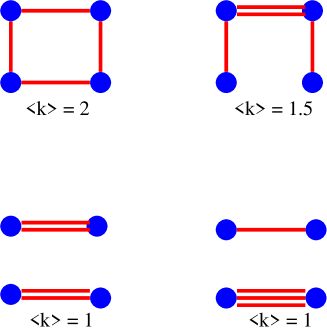
Figure 8: (Color online) Example of decrease of average degree with four nodes and four links. It is shown how average degree decreases as repeated interaction between agents take place leading to dimerisation.

Activity distribution is similar to model A and does not show any special feature.

The data for $d(m)$, average degree of an agent with wealth $m$ is shown in Fig. 9.

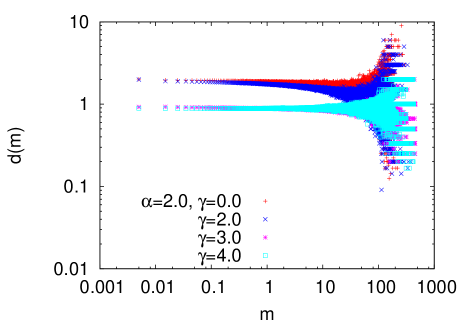
Figure 9: (Color online) Plot of $P_{d}(m)$ as a function of $m$ for model B with parameters $\alpha=2.0$, $\gamma=0.0,2.0,3.0,4.0$ and $N=1024$.

It is seen that $d(m)$ is again independent of the amount of wealth possessed by an agent (for $m\lesssim 1$) as in model A but can assume only two different values close to 1 and 2. $d(m)\simeq 1$ corresponds to a larger $\gamma$ value when dimerisation occurs.

Type of the model	$\alpha$	$\beta$	$\gamma$	$\nu$
Model B	$2.0$	$0.0$	$1.0$	$0.088$
	$2.0$	$0.0$	$2.0$	$0.096$
	$2.0$	$0.0$	$3.0$	$0.279$
	$2.0$	$0.0$	$4.0$	$0.174$
Model C	$3.0$	$1.0$	$0.0$	$0.798$
	$3.0$	$2.0$	$0.0$	$1.432$
	$3.0$	$3.0$	$0.0$	$2.134$
Model D	$2.0$	$1.0$	$1.0$	$0.671$
	$2.0$	$1.0$	$2.0$	$0.400$
	$2.0$	$1.0$	$3.0$	$0.091$
	$3.0$	$1.0$	$1.0$	$0.792$
	$3.0$	$1.0$	$2.0$	$0.519$
	$3.0$	$1.0$	$3.0$	$0.196$
	$3.0$	$3.0$	$2.0$	$2.34$

Table 1: Different values of Pareto Exponent for different combinations of $\alpha$, $\beta$ and $\gamma$.

III.3 Model C

In model C, the first agent $i$ is chosen with a probability $p_{i}=m_{i}^{\beta}$, where $\beta$ is a parameter. Chakraborty et. al. manna1 in a recent paper used such a preferential selection rule using a pair of continuously tunable parameters upon traders with distributed saving propensities and were able to reproduce the trend of enhanced rates of trading of the rich. The wealth distribution was found to follow Pareto law. However, in model C, we choose only the first agent with a preferential selection rule. The second agent is chosen with higher probability when she is financially close to the first as in models A and B. The interaction in model C occurs with a probability $P_{ij}$, given by,

$$P_{ij}\propto m_{i}^{\beta}|m_{i}-m_{j}|^{-\alpha}.$$ (5)

In effect, both the interacting agents are rich for higher value of $\alpha$.

The wealth distributions for two different values of $\alpha$ and various values of $\beta$ are shown in Fig. 10.

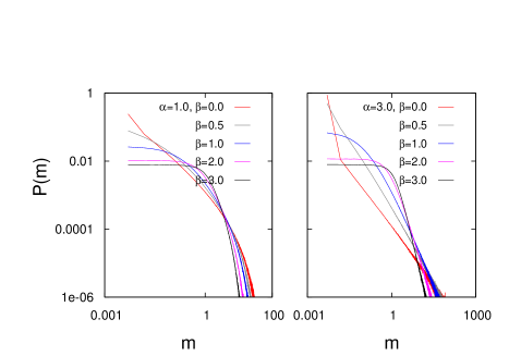
Figure 10: (Color online) Plot of $P(m)$ as a function of $m$ for model C with $N=1024$ and parameters $\alpha=1.0,3.0$ and for $\beta=0.0,0.5,1.0,2.0,3.0$.

It is seen that the wealth distribution is sufficiently altered for $\beta\neq 0$; a plateau/flat region is found for small $m$, and a power law region for a narrow range of $m$ follows it. It can be interpreted in the following way: as selection of the agents depend on their wealth, many agents may not interact at all. Now, poorer agents have less probabilities to interact. Thus the wealth distribution is almost flat up to a certain value of $m$. As agents become richer, they interact more and the form of wealth distribution shows variation with $m$. The exponent $\nu$ for the power law region is quite important here, because now it has an appreciable value $\nu\gtrsim 1$. As $\beta$ increases the value of $\nu$ also increases. For example, for a chosen set of parameters $\alpha=2.0,\beta=3.0$, the exponent $\nu$ has a value close to $2$. Pareto exponents for model C are shown in table 1.

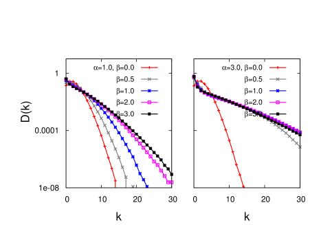
Figure 11: (Color online) Plot of degree distribution $D(k)$ as a function of degree $k$ for model C with $N=1024$ and parameters $\alpha=1.0$ and $3.0$ and for $\beta=0.0,0.5,1.0,2.0,3.0$.

Degree distribution in model C is more spread out compared to models A and B, as shown in Fig. 11. The plot indicates that for large $\alpha$, whatever value of $\beta$ we choose (except zero), we have a large number of agents with high degrees.

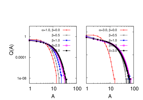
Figure 12: (Color online) Plot of activity distribution $Q(A)$ for model C with $N=1024$ and parameters $\alpha=1.0$ and $3.0$ and for $\beta=0.0,0.5,1.0,2.0,3.0$.

Here the activity distribution (Fig. 12) shows a distinct parameter dependence unlike models A and B. For large $\alpha$ and nonzero value of $\beta$, there is a considerably higher probability of large activity. As $\alpha$ and $\beta$ simultaneously help the interaction between rich agents to occur, for large value of $\alpha$ and nonzero $\beta$, interaction is limited within a ‘rich’group. These agents therefore enjoy large activity which is the reason why $Q(A)$ is nonzero for much larger values of $A$.

Average degree of an agent with wealth $m$, i.e., $d(m)$ is shown in Fig. 13.

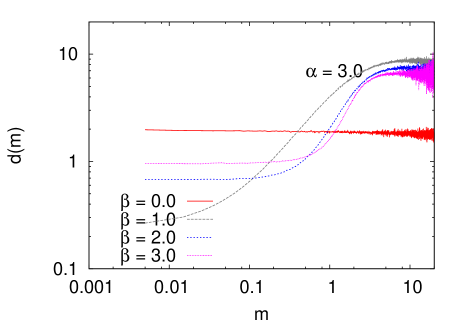
Figure 13: (Color online) Plot of $d(m)$ as a function of $m$ for model C with $N=1024$ and parameters $\alpha=3.0$, $\beta=0.0,0.5,1.0,2.0,3.0$.

It shows a different behaviour compared to models A and B. It is no longer a flat distribution. Richer agents have more neighbours as they have a priority in interactions resulting in an increasing trend in $d(m)$ with $m$ for large $m$.

IV Model D

In model D, we consider all the features contributed by the parameters $\alpha,\beta$ and $\gamma$. Here $P_{ij}$ can be written as,

$$P_{ij}\propto|m_{i}-m_{j}|^{-\alpha}m_{i}^{\beta}(c_{ij}+1)^{\gamma}$$ (6)

where $\beta=0,\gamma=0$ gives model A; $\beta=0$ gives model B and $\gamma=0$ gives model C.

The corresponding wealth distribution for model D is shown in Fig. 14. Note that as we increase $\gamma$ beyond $1$, the flat region disappears.

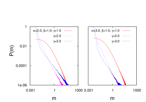
Figure 14: (Color online) Plot of $P(m)$ as a function of $m$ for model D with $N=1024$ and parameters $\alpha=2.0,3.0,\beta=1.0$ and $\gamma=1.0,2.0,3.0$.

With the presence of all three parameters, the value of the exponent $\nu$ is close to $1$ when $\gamma$ is small and decreases as $\gamma$ increases. The different values of $\nu$ for different combination of the parameter values are shown in Table 1.

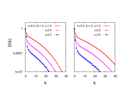
Figure 15: (Color online) Plot of $D(k)$ as a function of $k$ for model D with $N=1024$ and parameters $\alpha=2.0,3.0$, $\beta=1.0$ and for $\gamma=1.0,2.0,3.0$.

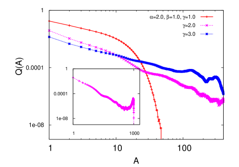
Figure 16: (Color online) Plot of activity distribution $Q(A)$ for model D with $N=1024$ and parameters $\alpha=2.0$, $\beta=1.0$ and for $\gamma=1.0,2.0,3.0$. The same plot for $\alpha=2.0,\beta=1.0,\gamma=2.0$ is shown for the whole range of activity in the inset showing the condensate like behaviour at large values of $A$.

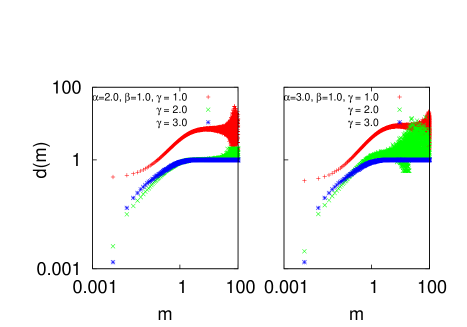
Figure 17: (Color online) Plot of $d(m)$ as a function of $m$ for model D with $N=1024$ and parameters $\alpha=1.0$, $\beta=3.0$ and for $\gamma=1.0,2.0,3.0$.

Here degree distribution has maximum value for $k=0$ and then drops off suddenly to a low value as shown in Fig. 15. The fall is sharper as $\gamma$ increases. Also note that with increasing $\alpha$, the degree distribution is more spread out as is also seen in Fig. 11. A feature similar to dimerisation as in model B is also observed here, but the average degree varies from $2$ to $0$ over a region of $\gamma$ unlike model B where the variation is from $2$ to $1$.

A striking feature is observed for activity distribution of model D. It can be seen that here with all the three parameters present, unless $\gamma$ is very small, the activity distribution shows power-law behaviour as shown in Fig. 16. The corresponding exponent is dependent on the value of the parameters and in general around 3 which is somewhat less than the observed value Gabaix . The power law behaviour of $Q(A)$ signifies the presence of a few agents with large amount of activity - evidently the rich agents have these property. In fact, for higher values of $\alpha$ and $\beta$, this effect is enhanced leading to the existence of a local peak at $A>>1$. However, the height of this peak is much lesser compared to $Q(A=1)$. This “condensation” type behaviour becomes more prominent for larger values of $\alpha$. Average degree $d(m)$ of an agent with wealth $m$ shows features similar to model C and is shown in Fig. 17.

V Comparison with real data

While modelling a particular system, e.g., as in GIori , one may calibrate the numerical simulations of the model with real data. Even for a general model, it is important that the exponent values of the relevant quantities obtained are comparable to real data. We have extracted the Pareto exponent and the exponent for the activity distribution wherever possible for the models proposed in this paper.

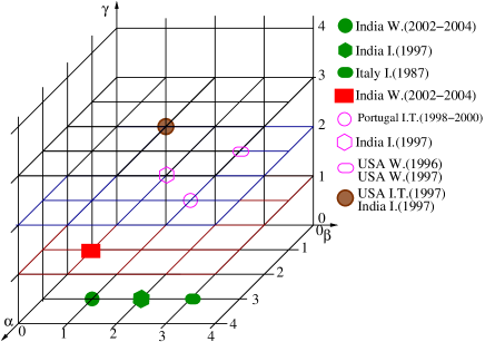
Figure 18: (Color online)3-d plot for the suitable values of $\alpha$, $\beta$ and $\gamma$ yeilding $\nu$ values corresponding to different coutries.

While considering real data, it is possible only to compare the Pareto exponents obtained from the different models. We therefore check for the values of $\alpha$, $\beta$ and $\gamma$ which give us a Pareto exponent $\nu$ comparable to the real data of several countries which appear in Pete_Rich . In Fig. 18, we show in a 3-d plot the suitable values of $\alpha$, $\beta$ and $\gamma$ yeilding $\nu$ values corresponding to different coutries. However, there is a word of caution - a particular real Pareto value may be obtained by more than one combination of $\alpha$, $\beta$ and $\gamma$ and one should not try to interpret the values shown in Fig. 18 to be optimum.

VI Summary and Discussions

To summarize, we have studied different wealth exchange models where agents interact via DY type interaction in addition to the fact the interactions among the agents are now preferential. For all the models we assume that two agents will interact only when they are “closely” located in the wealth space. This is controlled by the parameter $\alpha$ which is taken to be non-zero in all the models. The introduction of $\alpha$ leads to a power law behaviour in $P(m)$ above a certain value of $\alpha$ even without considering other factors like saving. To mimic the real situation we have also incorporated other parameters $\beta$ and $\gamma$. $\gamma$ takes care of the “memory” that a pair of agents have interacted already; probability of interaction increases with the number of past interactions controlled by the parameter $\gamma$. The parameter $\beta$ helps to select the agents with a probability proportional to their wealth. Although our prime concern is the wealth distribution, the issue of network formation has also been addressed by considering some fundamental network properties. In several earlier works, the question of network formation in financial systems has been considered Allen ; Babus .

With only $\alpha\neq 0$, one can get a power law decay in $P(m)$ with a Pareto exponent $\nu\approx 0.1$. With the introduction of either $\beta$ and/or $\gamma$, one still gets the power law decay but the value of $\nu$ shows drastic change. In principle it is possible to obtain a specific value of $\nu$ by properly tuning the parameters. When $\gamma$ is nonzero, an additional feature of dimerisation, observed in real data, appears in the results. However, the average degree does not show any significant dependence on the wealth possessed by an agent in models A and B (i.e. $\beta=0$). When $\beta$ is nonzero, the new feature which is observed is the nontrivial dependence of the average degree on the wealth of an agent, there being a distinct nonlinear increasing trend for higher values of $m$.

When all the three parameters are present (model D), one gets a power law for $\alpha\geq 2$ as in all the other models (A, B and C), and once again it is possible to generate various $\nu$ values by different combinations of $\alpha,\beta$ and $\gamma$ (Table 1). For model D, another desirable feature is obtained in addition to dimerisation and nontrivial variation of $d(m)$ with $m$. This is the power law observed in the activity distribution.

One has to carefully choose the values of $\alpha$, $\beta$ and $\gamma$ so as to achieve optimum behaviour in model D. We find that for $\alpha\sim 2,\beta\sim 1$ and $\gamma\sim 2$, the features become closest to reality. For example, making $\gamma$ large and $\beta$ small, the value of $\nu$ decreases, while for smaller values of $\gamma$ the activity $Q(A)$ does not show a power law behaviour. If $\beta$ is chosen as $>1$, the plateau region in $P(m)$ extends over a larger region of $m$ which is an undesirable feature. While $\alpha>1$ ensures a power law behaviour in $P(m)$, making $\alpha$ too large in model D leads to enhanced condensation behaviour. It should be mentioned that finite size effects for all cases are negligible for system size for which the results are reported.

However the problem with these optimum values of the is that the Pareto exponent $\nu$ in this case is rather small ($\sim 0.4$). The activity distribution also has an exponent smaller than the observed one. To obtain better values of these exponents one might try further fine tunings and incorporate features like saving.

Acknowledgement: Discussion with S. S. Manna during the initial formulation of the problem is acknowledged. PS is thankful to CSIR grant for financial support.

References

- (1) V. Pareto, Cours d’economie Politique, F. Rouge, Lausanne (1897).
- (2) B. B. Mandelbrot, Int. Econ. Rev. 1, 79 (1960).
- (3) B. K. Chakrabarti, A. Chakraborti, S. R. Chakravarty, A. Chatterjee, Econophysics of Income and Wealth Distributions (Cambridge University Press, Cambridge, 2013)
- (4) Econophysics of Wealth Distributions, edited by A. Chatterjee, S. Yarlagadda, B. K. Chakrabarti (Springer Verlag, Milan, 2005).
- (5) Econophysics and Sociophysics, edited by B. K. Chakrabarti, A. Chakraborti, A. Chatterjee (Wiley-VCH, Berlin, 2006).
- (6) S. Sinha, A. Chatterjee, A. Chakraborti, B. K. Chakrabarti, Econophysics: An Introduction (Wiley-VCH, Berlin, 2010).
- (7) V. M. Yakovenko, J. Barkley Rosser, Jr., Rev. Mod. Phys. 81, 1703 (2009).
- (8) A. C. Silva, V. M. Yakovenko, Europhys. Letts., 69, 304 (2005); A. A. Drăgulescu, V. M. Yakovenko, Eur. Phys. J. B, 20, 585 (2001); A. A. Drăgulescu, V. M. Yakovenko, Physica A 299, 213 (2001); M. Levy, S. Solomon, Physica A 242, 90 (1997); S. Sinha, Physica A 359, 555 (2006); H. Aoyama, W. Souma, Y. Fujiwara, Physica A 324, 352 (2003); T. Di Matteo, T. Aste, S. T. Hyde, in The Physics of Complex Systems (New Advances and Perspectives), edited by F. Mallamace, H. E. Stanley (IOS Press, Amsterdam, 2004); F. Clementi, M. Gallegati, Physica A 350, 427 (2005); N. Ding, Y. Wang, Chinese Phys. Letts., 24, 2434 (2007).
- (9) B. K. Chakrabarti, S. Marjit, Ind. J. Phys. B 69, 681 (1995); S. Ispolatov, P. L. Krapivsky, S. Redner, Eur. Phys. J. B 2, 267 (1998).
- (10) A. A. Drăgulescu, V. M. Yakovenko, Eur. Phys. J. B 17, 723 (2000).
- (11) A. Chakraborti, B. K. Chakrabarti, Eur. Phys. J. B 17, 167 (2000).
- (12) A. Chatterjee, B. K. Chakrabarti, Eur. Phys. J. B 60, 135 (2007); A. Chatterjee, S. Sinha, B. K. Chakrabarti, Current Science 92, 1383 (2007).
- (13) A. S. Chakrabarti, B. K. Chakrabarti, Economics E-journal, 4 (2010): http://www.economics-ejournal.org/economics/journalarticles/2010-4.
- (14) A. Chatterjee, in Mathematical Modeling of Collective Behavior in Socio-Economic and Life Sciences, edited by G. Naldi et. al. (Birkhaüser, Boston, 2010).
- (15) M. Patriarca, A. Chakraborti, K. Kaski, Phys. Rev. E 70, 016104 (2004).
- (16) P. Repetowicz, S. Hutzler, P. Richmond, Physica A 356, 641 (2005).
- (17) M. Lallouache, A. Jedidi, A. Chakraborti, arxiv:1004.5109v2.
- (18) J. Angle, Social Forces 65, 293 (1986); Physica A 367, 388 (2006).
- (19) A. Chatterjee, B. K. Chakrabarti, S. S. Manna, Physica A 335, 155 (2004); Phys. Scr. T 106, 36 (2003).
- (20) D.Garlaschelli, M.I. Loffredo, J. Phys. A : Math Theor. 41, 224018 (2008).
- (21) D. Sornette, R. Cont, J. Phys. I 7, 431 (1997).
- (22) S. Solomon, P. Richmond, Physica A 299, 188 (2001).
- (23) O. Malcai, O. Biham, P.Richmond, S. Solomon, Phys. Rev. E 66, 031102 (2002).
- (24) F. Allen and A. Babus in The Network Challenge, edited by P.R. Kleindorfer and Y. (Jerry) Wind with R. E. Gunther (Wharton School Publishing, New Jersey, 2009).
- (25) A. Babus, Fondazione Eni Enrico Mattei Working Papers, 129 (2007).
- (26) V. Hatzopoulos, G. Iori, R. N. Mantegna, S. Micciche, M. Tumminello, Discussion Paper Series 13/14 Department of Economics, City University London (2013).
- (27) M. Tumminello, F. Lillo, J. Piilo, R. N. Mantegna, New Journal of Physics 14, 013041 (2012).
- (28) X. Gabaix, P. Gopikrishnan, V. Plerou, H. E. Stanley, MIT Working Paper Series 3-30, 1 (2003).
- (29) A. Chakraborty, S. S. Manna, Phys. Rev. E 81, 016111 (2010).
- (30) G. Iori , R. N. Mantegna, L. Marotta, S. Miccichè, J. Porter and M. Tumminello, arXiv:1403.3638
- (31) P. Richmond, S. Hutzler, R. Coelho and P. Repetowicz in ESTP .