Effects of Lifshitz Transition on Charge Transport in Magnetic Phases of Fe-Based Superconductors

Abstract

The unusual temperature dependence of the resistivity and its in-plane anisotropy observed in the Fe-based superconducting materials, particularly Ba(Fe_1-xCo_x)₂As₂, has been a long-standing puzzle. Here, we consider the effect of impurity scattering on the temperature dependence of the average resistivity within a simple two-band model of a dirty spin density wave metal. The sharp drop in resistivity below the Néel temperature $T_{N}$ in the parent compound can only be understood in terms of a Lifshitz transition following Fermi surface reconstruction upon magnetic ordering. We show that the observed resistivity anisotropy in this phase, arising from nematic defect structures, is affected by the Lifshitz transition as well.

Lifshitz transitions (LT) in metals lifshitz , where Fermi surfaces change topology, have mostly been studied as zero temperature ($T$) phenomena driven by external parameters such as doping and pressure, etc. lifshitz2 ; buhmann . Temperature driven LT that can occur in spin or charge density wave phases of metals have received comparatively less attention. In this context, an interesting aspect of the Fe-based superconductors (FeSC) is their multiband nature with several hole and electron pockets. After band reconstruction in the spin density wave (SDW) phase, some of these pockets can disappear due to the increase of the SDW potential with lowering temperature. Recently, a combined study of electron Raman and Hall conductivity on SrFe₂As₂ has reported signatures of such a transition gallais2014 . This motivates us to study the effects of such transitions on the charge transport of the FeSC. Using a model where current relaxation is due to impurity scattering, we find remarkably strong signatures of such transitions in both the average resistivity $\rho_{avg}$ and the resistivity anisotropy $\rho_{ani}$ that are consistent with known experimental trends of these quantities.

The charge transport properties of the FeSC, particularly of BaFe₂As₂, are currently the subject of intense research. The $ab$-plane anisotropy of the resistivity $\rho_{ani}\equiv\rho_{a}-\rho_{b}$ of the strain detwinned crystals below the structural transition temperature $T_{S}$ has an intriguing sign with the shorter $b$ axis being more resistive than the longer $a$ axis tanatar ; chu ; chu2 . The anisotropy weakens upon entering the SDW phase even though the magnetic order by itself breaks $C_{4}$ symmetry. Furthermore, the anisotropy magnitude in the SDW phase typically increases upon light doping. Together with other measurements kim11 ; yi11 ; yi12 ; zhang12 ; zhao ; nakajima ; gallais2013 ; kasahara ; lgreene , substantial $\rho_{ani}$ has been taken as strong evidence for intrinsic electronic nematic behavior hu12 ; fernandes12 ; chubukov_fernandes_review14 . The behavior of the average resistivity $\rho_{avg}$, which has received considerably less attention, is also highly unusual rullier-albanque . In the parent compounds and lightly doped systems, $\rho_{avg}$ falls abruptly below the SDW transition at $T_{N}$, in dramatic contrast with conventional SDW systems such as Cr.

Several theoretical works have attempted to explain the origin of $\rho_{ani}$ based on either anisotropic inelastic scattering with spin fluctuations giving rise to hot spot physics fernandes-schmalian11 ; Prelovsek ; Brydon or on an anisotropic Drude weight of the carriers dagotto_prl ; valenzuela . Note that, in the 122 systems, where the anisotropy has mostly been studied, the band structure poses an additional challenge, since the ellipticity of the electron pockets vary along the $k_{z}$ axis; the ellipticity at $k_{z}=0$ and $\pi$ planes have opposite signs SuppMat . Consequently, in theories where the sign of $\rho_{ani}$ is determined by the ellipticity $\xi_{e}$ of the electron pockets on each $k_{z}$ plane, such as those involving spin fluctuation scattering, at least a partial cancelation is expected after the $k_{z}$ average, and the total $\rho_{ani}$ will depend on details of the band structure.

In contrast, to the best of our knowledge, there is no theory of the characteristic drop in the average resistivity $\rho_{avg}\equiv(\rho_{a}+\rho_{b})/2$ immediately below $T_{N}$. Clearly, it is important to simultaneously account for this unusual feature of $\rho_{avg}$ in addition to $\rho_{ani}$. A drop in the inverse Drude weight below $T_{N}$ has been recovered in simulations dagotto_prl and ab initio calculations blomberg , but this quantity is distinct from the resistivity and includes no information about the scattering mechanism. Qualitatively, the sharp drop in $\rho_{avg}$ below $T_{N}$ can be understood in terms of a collapse in the scattering rate due to the decrease in phase space upon partial gapping of the Fermi surface, which then overcompensates the loss of carriers. However, since these two competing effects have the same physical origin, namely the growth of the SDW amplitude with decreasing $T$, the challenge here is to understand why the scattering rate collapse dominates the resistivity, at least in the undoped and lightly doped compounds, and whether this collapse is dominated by the elastic or inelastic scattering channel.

Our focus on impurity scattering can be appreciated from Fig. 1(a), where we fit the resistivity data of BaFe₂As₂ from Ref. ishida13, in the high-$T$ paramagnetic phase ($T>T_{N}\approx 141\mathrm{\;K}$) to $\rho_{avg}=A+BT^{2}$. We find excellent agreement up to $T\approx 300\mathrm{\;K}$, which argues in favor of conventional Fermi liquid and disorder scattering, rather than bad-metal physics bad-metal . More importantly, we find that $A\gg BT_{N}^{2}$ by an order of magnitude, implying that already at $T_{N}$ the elastic scattering from impurities dominates over inelastic processes.

The relevance of impurity scattering to explain $\rho_{ani}$ is currently being debated. Recently, Ishida et al. ishida13 reported that, upon annealing, $\rho_{ani}$ of BaFe₂As₂ nearly vanished, while significant anisotropy remained in Co-doped compounds. They argued that $\rho_{ani}$ is due to “nematogens” or anisotropic scattering potentials induced by Fe vacancies and Co defects. Such spatially extended defects aligned preferentially along $a$ direction have also been reported by scanning probe studies chuang10 ; allan13 ; grothe12 ; song11 ; song12 ; hanaguri12 ; zhou11 ; rosenthal13 . From the theoretical standpoint, $C_{4}$ symmetry breaking defect structures around pointlike impurities driven by orbital kontani or spin navarro ; navarro_nem correlations have indeed been found in realistic models of the Fe-based materials. On the other hand, Kuo and Fisher kuo14 , from a comparison of Co and Ni doped samples, have argued that the strain induced $\rho_{ani}$ does not depend on impurity concentration and therefore is an intrinsic property of the carriers.

The following are our main results. (i) We show that the characteristic drop in $\rho_{avg}(T)$ in the SDW phase is a consequence of one or more temperature-driven LT. (ii) The result applies to a multiband system in a “dirty” limit, in which an effective elastic scattering rate $\Gamma>W_{0}$, where $W_{0}$ is SDW potential at $T=0$. In the opposite limit, $\rho_{avg}(T)$ increases in the SDW phase. (iii) Consistent with our earlier study navarro_nem , we find that extended anisotropic impurity states aligned along $a$ direction give rise to $\rho_{ani}<0$ in the paramagnetic state. More importantly, we show that the anisotropy is independent of the ellipticity of the electron pockets provided the scattering is dominantly intraband. (iv) For parameters relevant for the parent compound, the LT produce a drop in $\rho_{ani}(T)$ below $T_{N}$ which is consistent with experiments. This feature is suppressed by reducing $W_{0}$ sufficiently, which is in qualitative agreement with the measured doping dependence of $\rho_{ani}(T\rightarrow 0)$.

Model.—We consider the two-band model of Brydon et al. pBrydon11 along with a mean field description of the SDW state and introduce intraband impurity scattering. Since our goal is to study the effect of rapid change of density of states due to a $T$-driven LT, we do not expect orbital physics to affect the results qualitatively. The Hamiltonian is given by ${\mathcal{H}}={\mathcal{H}}_{c}+{\mathcal{H}}_{f}+{\mathcal{H}}_{\text{SDW}}+{\mathcal{H}}_{\text{imp}}$. Here, ${\mathcal{H}}_{c}=\sum_{{\mathbf{k}},\sigma}\varepsilon^{c}_{{\mathbf{k}}}c^{\dagger}_{{\mathbf{k}},\sigma}c_{{\mathbf{k}},\sigma}$ and ${\mathcal{H}}_{f}=\sum_{{\mathbf{k}},\sigma}\varepsilon^{f}_{{\mathbf{k}}}f^{\dagger}_{{\mathbf{k}},\sigma}f_{{\mathbf{k}},\sigma}$ describe $c$-hole and $f$-electron bands, with spin $\sigma$, centered around $\Gamma$ and $X/Y$ points of the 1Fe/cell Brillouin zone (BZ) with dispersions $\varepsilon_{\mathbf{k}}^{c}=\varepsilon_{c}+2t_{c}(\cos k_{x}+\cos k_{y})$ and $\varepsilon_{\mathbf{k}}^{f}=\varepsilon_{f}+t_{f1}\cos k_{x}\cos k_{y}-t_{f2}\xi_{e}(\cos k_{x}+\cos k_{y})$, respectively. ${\mathcal{H}}_{\text{SDW}}=\sum_{{\mathbf{k}},\sigma}\sigma Wc^{\dagger}_{{\mathbf{k}},\sigma}f_{{\mathbf{k}}+{\mathbf{Q}},\sigma}+\text{H.c.}$, with ${\mathbf{Q}}=(\pi,0)$. SDW potential $W=W_{0}\tanh(2\sqrt{T_{N}/T-1})$ for $T\leq T_{N}$ and zero otherwise. We specify all energies in units of $t_{c}$, and we choose $\varepsilon_{c}=-3.5$, $\varepsilon_{f}=3.0$, $t_{f1}=4.0$, $t_{f2}=1.0$, $T_{N}=0.04$. Depending on the magnitude of $W_{0}$, there are either no LT ($W_{0}<W_{e}^{\ast}$), or one LT ($W_{h}^{\ast}>W_{0}>W_{e}^{\ast}$) where electron pockets disappear below $T<T_{e}^{\ast}$, or two transitions ($W_{0}>W_{h}^{\ast}$) where, in addition, hole pockets disappear below $T<T_{h}^{\ast}<T_{e}^{\ast}$. ($W_{e}^{\ast},W_{h}^{\ast},T_{e}^{\ast},T_{h}^{\ast}$) depend on the dispersion parameters.

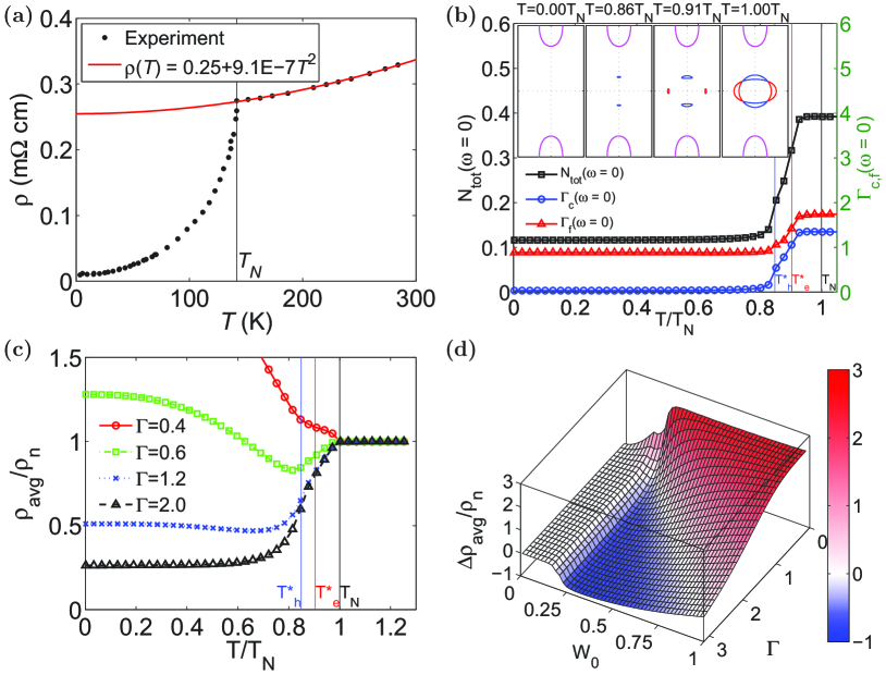
Figure 1: (color online). (a) Fit (red line) of resistivity data (black dots) from Ref. ishida13, in the high-$T$ paramagnetic phase with $\rho_{avg}=2.5\times 10^{-1}+9.1\times 10^{-7}T^{2}$. (b) $T$ evolution of the total density of states and the $c$- and $f$-electron scattering rates. Insets: Fermi surface evolution due to $T$ dependence of SDW potential. $T_{N}$, $T_{e}^{*}$, $T_{h}^{*}$ are defined in text. (c) $T$ dependence of average resistivity for various total scattering rates $\Gamma$. $\rho_{n}\equiv\rho_{avg}(T=T_{N})$. (d) $\Delta\rho_{avg}$ (defined in text) dependence on $W_{0}$ and $\Gamma$.

The impurity potential ${\mathcal{H}}_{\text{imp}}=\sum_{{\mathbf{k}},\mathbf{q},\sigma}V_{\mathbf{q}}c^{\dagger}_{{\mathbf{k}},\sigma}c_{{\mathbf{k}}+\mathbf{q},\sigma}+(c\rightarrow f)$, with $V_{\mathbf{q}}=V_{0}+V_{1}(1+2\cos q_{x})$, describes scattering of electrons with both isotropic pointlike ($V_{0}$ term) and anisotropic extended impurity ($V_{1}$ term) potentials. The latter is modeled by three pointlike scatterers aligned along the long or antiferromagnetic $a$ direction ($x$ axis), and constitutes $T$-independent analogs of the emergent nematogens reported in Ref. navarro_nem, . In the BaFe₂As₂ system, $V_{0}$ might represent weak out of plane disorder not capable of generating nematogens navarro ; navarro_nem , and $V_{1}$ strong in-plane scatterers like Fe vacancies.

We treat the impurity scattering in the Born approximation, and calculate the $c$ and $f$-scattering rates $\Gamma^{c}_{{\mathbf{k}}}(\omega)=-\operatorname{Im}[n_{i}\sum_{{\mathbf{k}}^{\prime}}|V_{{\mathbf{k}}-{\mathbf{k}}^{\prime}}|^{2}G_{{\mathbf{k}}^{\prime}{\mathbf{k}}^{\prime}}^{cc}(\omega)]$ where $n_{i}$ is the impurity concentration, and similarly $\Gamma^{f}_{{\mathbf{k}}}(\omega)$, respectively. We parameterize the two impurity potentials by defining the scattering rates $\Gamma\equiv n_{0}V_{0}^{2}N_{\text{tot}}$ and $\Gamma_{1}\equiv n_{1}V_{1}^{2}N_{\text{tot}}$, where $(n_{0},n_{1})$ are the concentrations of pointlike and extended impurities, respectively, and $N_{\text{tot}}$ is the total density of states at the chemical potential. Note that, due to $c$-$f$ mixing in the SDW phase, the Green’s functions acquire double indices. Here, $G^{cc}$, $G^{ff}$, etc., denote retarded Green’s functions in the absence of disorder. In other words, we do not calculate the scattering rates self-consistently, but we checked that doing so does not change the results significantly. We ignore the real parts of these diagonal (in $c$-$f$ basis) self energies since our aim is only to extract lifetime effects from the impurity scattering. Similarly, we do not intend to study how impurity scattering affects the SDW potential, and consequently, we ignore impurity induced off diagonal self energies. We calculate the conductivity in units of $e^{2}/\hbar$

$$\sigma_{ii}=-2\sum_{{\mathbf{k}}\in\text{BZ}}\int_{-\infty}^{\infty}\frac{d\omega}{\pi}\frac{\partial n_{\text{F}}(\omega)}{\partial\omega}\Big{\{}[2v^{c}_{{\mathbf{k}},i}\operatorname{Im}\bar{G}^{cc}_{{\mathbf{k}}{\mathbf{k}}}(\omega)]^{2}+$$

$$[v^{f}_{{\mathbf{k}},i}\operatorname{Im}\bar{G}^{ff}_{{\mathbf{k}}{\mathbf{k}}}(\omega)]^{2}+4v^{c}_{{\mathbf{k}},i}v^{f}_{{\mathbf{k+Q}},i}[\operatorname{Im}\bar{G}^{cf}_{{\mathbf{k}}{\mathbf{k+Q}}}(\omega)]^{2}\Big{\}},$$ (1)

where $\bar{G}$ represent the impurity dressed Green’s functions, $v_{{\mathbf{k}}}^{c,f}$ the velocity vectors, and $i$ is the $(a,b)$ component of the conductivity tensor $\overleftrightarrow{\sigma}$ (which is diagonal by symmetry). The factor 2 before $v_{{\mathbf{k}}}^{c}$ in the brackets accounts for two hole pockets at $\Gamma$.

Note that $\rho_{avg}(T)$ and $\rho_{ani}(T)$ are $T$ independent in the paramagnetic phase of this model, while the main $T$ dependence in the SDW phase is due to that of the potential $W(T)$. By contrast, in experiment $\rho_{ani}$ is peaked near $T_{N}$ ishida13 . In Ref. navarro_nem, , we argued that this $T$-dependent anisotropy is intimately related to the unusual nature of the nematogens, whereby they grow in size as the system approaches $T_{N}$. In the current Letter of the effects of LT, we ignore this $T$ dependence for simplicity.

Average resistivity.—We compute first $\rho_{avg}(T)$ by considering only pointlike impurities ($V_{1}=0$). In this case, changing the sign of the ellipticity $\xi_{e}\rightarrow-\xi_{e}$ is approximately equivalent to $\rho_{a}\leftrightarrow\rho_{b}$ so $\rho_{avg}(T)$ is unchanged (see below). Thus, we compute it reliably for a given ellipticity, which we fix to $\xi_{e}=2$. In Figs. 1(b)–1(c) we take $W_{0}=0.32$ with $W_{0}/T_{N}=8$ (consistent with optical measurements deGiorgi ; Hu2008 ), such that $W_{0}>W_{h}^{\ast}$. The Fermi surface reconstructions associated with the two LT as a function of $T$ are shown in the inset of Fig. 1(b). The main panel of (b) shows rapid drops in $N_{\text{tot}}(\omega=0)$ and in the scattering rates $\Gamma_{c,f}(\omega=0)$, which is expected from the loss of Fermi surface sheets associated with the LT. These two competing trends define a crossover in the $T$ dependence of $\rho_{avg}(T)$ which is shown in Fig. 1(c). For small $\Gamma\ll W_{0}$ (clean limit), the loss of carriers dominates and the resistivity increases with lowering $T$. But for large $\Gamma\gg W_{0}$ (dirty limit), the decrease in the scattering rates dominates, and results in a drop in $\rho_{avg}(T)$ whose magnitude for $\Gamma=2$ is comparable to that of the parent compounds. Note that this scenario of enhanced conductivity due to increased lifetime, as opposed to that due to enhanced Drude weight dagotto_prl , is consistent with optical measurements deGiorgi ; Hu2008 . Furthermore, at $T=0$ we get $\Gamma_{c}(\omega=0)\ll W_{0}$ [see Fig. 1(b)], which agrees with optical conductivity measuring the Drude peak and the spectral weight depletion due to SDW as well-separated features in frequency deGiorgi ; Hu2008 , while the remaining $\Gamma_{f}(\omega=0)$ contributes to a broad background.

Next, we define the net change in average resistivity $\Delta\rho_{avg}\equiv\rho_{avg}(T=0)-\rho_{avg}(T=T_{N})$ and show how it varies with $\Gamma$ and $W_{0}$ in Fig. 1(d). For $W_{0}<W_{e}^{\ast}$, there is no LT and the change is negligible. For $W_{0}>W_{e}^{\ast}$, such that the system undergoes at least one LT, we see clearly the dirty (where $\Delta\rho_{avg}<0$) to clean (where $\Delta\rho_{avg}>0$) crossover as $\Gamma$ is changed for fixed $W_{0}$. This implies that $\rho_{avg}(T)$ of undoped or lightly-doped compounds can be explained by a LT provided $W_{e}^{\ast}<W_{0}<\Gamma$.

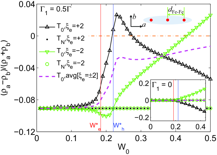
Figure 2: (color online). Main panel: $\rho_{ani}$ vs. SDW gap $W_{0}$ for $\Gamma_{1}=0.5\Gamma$. Curves for ellipticity $\xi_{e}=\pm 2$ at $T=T_{0}=0$ (upward or downward triangles, respectively) and at $T=T_{N}$ (dots or circles, respectively), and for the average of two-plane model (dashed line). The dash-dotted line indicates $\rho_{ani}=0$. $W_{e}^{\ast}$, $W_{h}^{\ast}$ are defined in text. Bottom inset: same quantities for $\Gamma_{1}=0$. Top inset: cartoon of extended impurity potential aligned along antiferromagnetic axis $a$.

Resistivity anisotropy.—We model the Fermi surface of the 122 systems by calculating the contributions to the conductivity from the planes $k_{z}=\pi\;(0)$ with their dispersions differing only in the $f$-band ellipticities $\xi_{e}=2\;(-2)$. We calculate the resistivity anisotropy of the planes $\rho_{ani,\xi_{e}}\equiv\rho_{a,\xi_{e}}-\rho_{b,\xi_{e}}$ separately, and then the experimentally relevant net anisotropy $\rho_{ani}={\bar{\rho}}_{a}-{\bar{\rho}}_{b}$ from the average of the conductivities of the two planes, i.e., $\bar{\rho}_{i}=\langle\sigma_{i}(k_{z})\rangle_{k_{z}}^{-1}\simeq 2/(\rho_{i,\xi_{e}}^{-1}+\rho_{i,-\xi_{e}}^{-1})$, where $\langle\rangle_{k_{z}}$ is the exact integral over $k_{z}$, which we have approximated by the average of the contributions at $k_{z}=0$ and $\pi$. As noted earlier for $\Gamma_{1}=0$, since $\xi_{e}\rightarrow-\xi_{e}$ leads approximately to $\rho_{a}\leftrightarrow\rho_{b}$, the net anisotropy $\rho_{ani}\simeq 0$ for $T<T_{N}$, as seen in experiments on annealed samples ishida13 , even though the SDW state itself breaks $C_{4}$ symmetry (see Fig. 2 bottom inset). The real BaFe₂As₂ Fermi surface is considerably more complicated, and there is no exact cancellation between the contributions of $k_{z}=0$ and $\pi$ to $\rho_{ani}$, but the true $\rho_{ani}$ will nevertheless be considerably reduced due to $k_{z}$ averaging.

We now consider nematogen scattering by setting $\Gamma_{1}=0.5\Gamma$, and calculate the anisotropies both in the paramagnetic and the SDW phases. Figure 2 shows $\rho_{ani,\xi_{e}}$ and $\rho_{ani}$ at $T=T_{N}$ and $0$ for a wide range of $W_{0}$. We note that both $\rho_{ani}(T_{N})<0$ and $\rho_{ani}(0)<0$, consistent with experiments. The physical implication of the negative sign is that the nematogens, being aligned along the $a$ direction, scatter more carriers moving along $b$ than those moving along $a$. Consequently, we expect this feature to hold even in the presence of interband impurity scattering. Next, we note that $\rho_{ani,\xi_{e}}(T_{N})$ is independent of the sign of $\xi_{e}$, which can be understood as follows. In the paramagnetic phase, assuming intraband-only scattering, the $c$- and $f$-bands decouple. Consequently, shifting only the $f$ band by $(\pi,\pi)$, keeping the $c$ band unshifted, is an allowed unitary transformation. $\rho_{ani,\xi_{e}}(T\geq T_{N})$ is invariant under this transformation mapping $\xi_{e}\rightarrow-\xi_{e}$ and is thus independent of the sign of $\xi_{e}$.

Strictly speaking, this argument is invalid in the SDW phase due to $c$-$f$ mixing. Nevertheless for $W_{0}\ll W_{e}^{\ast}$ (relevant for sufficiently doped systems), i.e., without any LT, the Fermi surface reconstruction is rather weak and we find that $\rho_{ani,\xi_{e}}(0)$ is practically independent of the sign of $\xi_{e}$, and, moreover, $\rho_{ani,\xi_{e}}(0)\approx\rho_{ani}(0)\approx\rho_{ani}(T_{N})$. However, for $W_{0}>W_{e}^{\ast}$, the Fermi surface reconstruction due to the LT is significant, and $\rho_{ani,2}(0)$ and $\rho_{ani,-2}(0)$ are generally different. On the other hand, the magnitude of the net anisotropy is always less than that in the paramagnetic state, i.e., $\left|\rho_{ani}(0)\right|<\left|\rho_{ani}(T_{N})\right|$. This is due to loss of $N_{\text{tot}}(\omega=0)$ accompanying the LT (presumably, the associated gain in carrier lifetime does not affect $\rho_{ani}$). Thus, the LT scenario is able to explain why the resistivity anisotropy of the undoped and lightly doped systems decrease as one goes below $T_{N}$ in the SDW phase even though the SDW itself breaks $C_{4}$ symmetry. Furthermore, for $W_{0}<W_{h}^{\ast}$, $\left|\rho_{ani}(0)\right|$ increases with decreasing $W_{0}$, which is consistent with the observation that the resistivity anisotropy in the SDW phase increases with sufficient doping footnote-valenzuela . Finally, in Fig. 3 we show the $T$ dependence of $\rho_{ani,\xi_{e}}(T)$ and $\rho_{ani}(T)$ for $W_{0}=0.2$ (intermediate doping) with $W_{0}/T_{N}=8$.

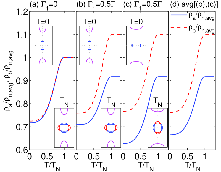
Figure 3: (color online). (a) Resistivity $\rho_{a,b}$ at $k_{z}=\pi$ for a two-plane model with isotropic scatterers. (b)–(c) Same at $k_{z}=\pi,0$, respectively, for a two-plane model with anisotropic scatterers. (d) Average of (b) and (c).

Conclusions.—We studied how $T$-driven Lifshitz transitions, where Fermi pockets disappear due to an increasing SDW potential, affect the average resistivity $\rho_{avg}$ and its anisotropy $\rho_{ani}$ of FeSC in the magnetic phase. By fitting experimental data, we argued that the dominant current relaxation mechanism in these materials is impurity scattering. We considered both pointlike and extended impurity (nematogen) potentials, and showed that the characteristic drop in $\rho_{avg}(T)$ is due to Lifshitz transitions in a dirty SDW metal. Next, we showed that the nematogen generated $\rho_{ani}$ has the correct sign, namely the direction with longer lattice constant is less resistive. Within this model, the anisotropy in the paramagnetic phase is independent of the sign of the ellipticity of the electron pockets. In the SDW phase, the above holds approximately when the SDW potential is weak enough. The qualitative physics discussed here is general enough to be of potential interest for transport in other multiband systems showing density wave instabilities.

We thank M. Breitkreiz, R. Fernandes, Y. Gallais, J. Schmalian, and C. Timm for useful discussions. P.J.H. and Y.W. were partially supported by Grant NSF-DMR-1005625, B.M.A. and M.N.G. by Lundbeckfond fellowship (Grant No. A9318), and M.T., H.O.J. and R.V. were partially supported by the Deutsche Forschungsgemeinschaft through Grant No. SPP 1458.

I [Supplemental Information]

II BaFe₂As₂ Fermi surface by first-principles calculations

In this supplement, we consider the Fermi surface of magnetically ordered BaFe₂As₂ obtained from first-principles calculations using density functional theory (DFT) in order to provide background and justification for the simple 2-band Hamiltonian model given in the main text, with dispersions $\varepsilon^{c,f}_{\mathbf{k}}$ defined in the 1-Fe Brillouin zone (BZ). The 122 materials (including BaFe₂As₂) have a different symmetry than, e.g., the 1111 materials for which this Hamiltonian was developed, which requires accounting for the significant $k_{z}$ dependence of the Fermi surface. Specifically, the ellipticity $\xi_{e}$ of the electron pockets changes sign from $k_{z}=0$ to $k_{z}=\pi$, as suggested by the DFT calculations shown below. From the perspective of our calculation, $\xi_{e}$ within a purely 2D model cannot be fixed to one sign or the other without losing qualitative features of the electronic structure that are important for the Fermi surface anisotropy. To deal with this problem within a model framework, we consider the contributions to the conductivity from two representative planes $k_{z}=0,\pi$, each calculated from a 2D model Hamiltonian with different ellipticities in the dispersions $\varepsilon^{f}_{\mathbf{k}}$, as a realization of the 3D Fermi surface in the paramagnetic state (shown in Fig. S1(a) as calculated from FPLO koepernik1999 for the BaFe₂As₂ orthorhombic structure at $20\mathrm{\;K}$ ambient pressure rotter2008 ).

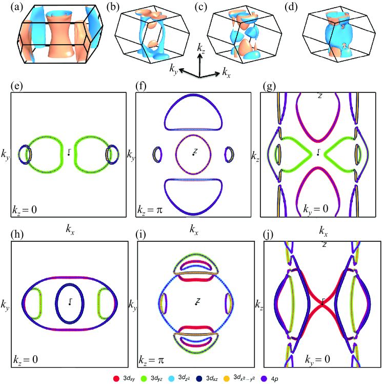
Figure S1: Fermi surface of BaFe₂As₂ in the paramagnetic phase in the BZ corresponding to the primitive cell of $Fmmm$ space group (a), in the antiferromagnetic phase in the BZ corresponding to the primitive cell of $Cccm$ space group with full DFT magnetic moments of $2.1\;\mu_{B}$ (b), and in the antiferromagnetic phase with the magnetic moments downscaled to $0.9\;\mu_{B}$ (c) and to $0.35\;\mu_{B}$ (d). Second row: cuts of antiferromagnetic Fermi surface in panel (c) for $k_{z}=0$ (e), $k_{z}=\pi$ (f), and $k_{y}=0$ (g). Third row: cuts of antiferromagnetic Fermi surface in panel (d) for $k_{z}=0$ (h), $k_{z}=\pi$ (i), and $k_{y}=0$ (j).

Below the Néel temperature $T_{N}$, the DFT ground state is known to display the stripelike magnetic order [$\mathbf{Q}=(\pi,\pi,0)$ in the 2-Fe zone], in agreement with experiment. As shown in Fig. S1(b), the magnetic ground state from the fully self-consistent DFT calculation exhibits a very strong reconstruction, such that any remnant of the simple magnetic folding shown in the right panel of the Fig. 1(b) insert in the main text would be hard to discern. However, this calculation gives an ordered antiferromagnetic moment of $2.1\;\mu_{B}$, which is known to exceed the actual ordered moment by a factor of 2 compared to experiment. Therefore we have performed the same calculation for a restricted moment corresponding to the experimentally measured value, $0.9\;\mu_{B}$ huang2008 and show the obtained 3D Fermi surface in Fig. S1(c) and, additionally, various cuts through this Fermi surface in Fig. S1(e)–(g). It is now clear that the reconstructions in the $k_{z}=0,\pi$ planes resemble those one would expect from folding the paramagnetic Fermi surface shown in Fig. S1(a), and those in the spin density wave state from our model in Fig. 1(b) in the main text. Furthermore, for comparison we show in Fig. S1(d) the 3D Fermi surface corresponding to an ordered moment of $0.35\;\mu_{B}$ where the reconstruction is minimal, and in Fig. S1(h)–(j) the various cuts through this Fermi surface.

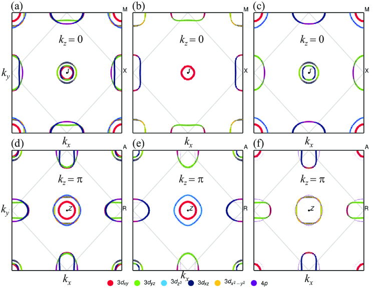
Figure S2: Ab initio Fermi surface and the unfolded Fermi surface. Top panels: $k_{z}=0$ cut; lower panels: $k_{z}=\pi$ cut. (a, d) Ab initio Fermi surface plotted 1Fe zone. The gray line shows the boundary of 2Fe zone. (b, e) Unfolded Fermi surface obtained by projecting the Bloch states onto the irreducible subspaces of the glide-mirror group corresponding to the representations $D^{({\mathbf{k}},+)}$. (c, f) as in former, only corresponding to $D^{({\mathbf{k}},-)}$. Note although the unit cell is orthorhombic, we use high symmetry point labels of the tetragonal unit cell for simplicity. The folding vector $(\pi,\pi,\pi)$ is apparent when top and bottom panels, e.g., (b) and (f), are compared.

The comparison with the model Fermi surfaces in the main text is not straightforward, however, since Fig. S1 corresponds to a 2-Fe unit cell representation in which the DFT calculations have been performed, whereas the calculations in the main text from our model use the 1-Fe unit cell. To properly represent the Fermi surfaces in a 1-Fe model, one should carefully unfold the bandstructure WeiKu ; Andersen2011 , a procedure which is nonintuitive in the complicated 122 crystal structure. It can be accomplished, however, using symmetries of the crystal in a formal group theoretic treatment tomic2014 . To illustrate our method, we show the ab initio Fermi surface [Fig. S2(a, d)] obtained from VASP vasp and unfolded Fermi surface [Fig. S2(b, c, e, f)] at $k_{z}=0$ and $k_{z}=\pi$ in Fig. S2(a)–(c) and Fig. S2(d)–(f), respectively. The ab initio Fermi surface corresponds to the primitive cell containing two translationally inequivalent Fe atoms, while the unfolded Fermi surface corresponds to the primitive cell containing one Fe atom. Since the crystal has the glide-mirror symmetry which dictates a degeneracy in the bandstructure, it is possible to divide the energy bands ($\varepsilon_{n,{\mathbf{k}}}$) unambiguously into two sectors ($\varepsilon_{+n,{\mathbf{k}}}$ and $\varepsilon_{-n,{\mathbf{k}}}$ defined in 1-Fe zone) that are connected by a folding vector ${\mathbf{k}}_{f}=(\pi,\pi,\pi)$ (i.e., $\varepsilon_{+n,{\mathbf{k}}}$ = $\varepsilon_{-n,{\mathbf{k}}+{\mathbf{k}}_{f}}$). (Note $\varepsilon_{n,{\mathbf{k}}}=\varepsilon_{n,{\mathbf{k}}+{\mathbf{k}}_{f}}$ is trivial since ${\mathbf{k}}_{f}$ is the reciprocal lattice vector of 2-Fe zone; it is the division of the $\varepsilon_{n,{\mathbf{k}}}$ in 2-Fe zone into $\varepsilon_{\pm n,{\mathbf{k}}}$ in 1Fe zone that is non-trivial and a manifestation of the glide-mirror symmetry.)

This opens up the possibility to formulate a simpler 1-Fe effective model with energy bands either $\varepsilon_{+n,{\mathbf{k}}}$ or $\varepsilon_{-n,{\mathbf{k}}}$, whose Fermi surface, when folded along ${\mathbf{k}}_{f}$, results in the Fermi surface shown in Fig. S2(a) and Fig. S2(d). In order to identify which portions of the Fermi surface correspond to the 1-Fe effective model we make use of group theory tomic2014 . Geometrically, we need to map the two translationally inequivalent irons onto each other by means of the glide-mirror operation and then construct the Bloch-like states adapted to the glide-mirror symmetry. Formally, this is achieved by projecting the Bloch-like states onto the irreducible subspaces of the glide-mirror group, which is just the translation group of the primitive cell of 122 materials extended by the glide-mirror operation. This extra operation reduces the number of independent degrees of freedom in the ab-initio electronic structure by a factor of two, allowing us to deduce the Fermi surface of the 1-Fe model. Specifically, the glide-mirror group has two one-dimensional irreducible representations on the $k_{z}=0$ and $k_{z}=\pi$ planes ($k_{z}=-\pi$ is equivalent to $k_{z}=\pi$), given by $D^{({\mathbf{k}},\pm)}({\hat{\mathrm{T}}}_{\mathbf{R}})=e^{-i{\mathbf{k}}\cdot{\mathbf{R}}}$ and $D^{({\mathbf{k}},\pm)}({\hat{\mathrm{G}}})=\pm e^{-i{\mathbf{k}}\cdot{\mathbf{\tau}}}$, where ${\hat{\mathrm{T}}}_{\mathbf{R}}$ is a translation by lattice vector ${\mathbf{R}}$ and ${\hat{\mathrm{G}}}$ is the glide-mirror operation, with ${\mathbf{\tau}}$ the vector connecting the two translationally inequivalent iron atoms. The corresponding glide-mirror symmetry adapted Bloch-like basis is generated by the action of projectors ${\hat{\mathrm{P}}}^{({\mathbf{k}},\pm)}=\sum_{{\hat{\mathrm{F}}}}D^{({\mathbf{k}},\pm)\dagger}({\hat{\mathrm{F}}}){\hat{\mathrm{F}}}$, where ${\hat{\mathrm{F}}}$ is an operation from the glide-mirror group. The irreducible representations $D^{({\mathbf{k}},+)}$ and $D^{({\mathbf{k}},-)}$ each contain one half of the bands from the two iron primitive cell and are related by the folding vector ${\mathbf{k}}_{f}$, i.e., $D^{({\mathbf{k}},-)}=D^{({\mathbf{k}}+{\mathbf{k}}_{f},+)}$, which means that each of the irreducible representations $D^{({\mathbf{k}},\pm)}$ represents one 1-Fe model with the needed folding vector. When the Fermi surface is unfolded according to this prescription, the ellipticity of the overlapping electron pockets can be unambiguously resolved and the unfolded Fermi surface shown in either Fig. S2(b, e) [from $D^{({\mathbf{k}},+)}$] or Fig. S2(c, f) [from $D^{({\mathbf{k}},-)}$] indicates the sign changing of the ellipticity of the electron pocket from $k_{z}=0$ to $k_{z}=\pi$ as we have assumed in our model [corresponding to Fig. S2(c, f)]. The realistic reconstructed Fermi surface, e.g., Fig. S1(c), is obviously considerably more complex than our two-plane model, but this model nevertheless captures the main qualitative point that the resistivity anisotropy due to isotropic point scatters will be generally considerably reduced by integration over the full 122 Fermi surface.

References

- (1) I. M. Lifshitz, Sov. Phys. JETP 11, 1130 (1960).
- (2) In the context of FeAs, see, e.g., C. Liu et al. Phys. Rev. B 84, 020509(R) (2011); K. Quader and M. Widom, Phys. Rev. B 90, 144512 (2014).
- (3) For a transport study, see, e.g., J. M. Buhmann and M. Sigrist, Phys. Rev. B 88, 115128 (2013).
- (4) Y.-X. Yang, Y. Gallais, F. Rullier-Albenque, M.-A. Measson, M. Cazayous, A. Sacuto, J. Shi, D. Colson, and A. Forget, Phys. Rev. B 89, 125130 (2014).
- (5) M. A. Tanatar, A. Kreyssig, S. Nandi, N. Ni, S. L. Bud’ko, P. C. Canfield, A. I. Goldman, and R. Prozorov, Phys. Rev. B 79, 180508 (2009).
- (6) J.-H. Chu, J. G. Analytis, K. De Greve, P. L. McMahon, Z. Islam, Y. Yamamoto, and I. R. Fisher, Science 329, 824 (2010).
- (7) J.-H. Chu, H.-H. Kuo, J. G. Analytis, and I. R. Fisher, Science 337, 710 (2012).
- (8) Y. K. Kim, H. Oh, C. Kim, D. Song, W. Jung, B. Kim, H. J. Choi, C. Kim, B. Lee, S. Khim, H. Kim, K. Kim, J. Hong, and Y. Kwon, Phys. Rev. B 83, 064509 (2011).
- (9) M. Yi, D. Lu, J.-H. Chu, J. G. Analytis, A. P. Sorini, A. F. Kemper, B. Moritz, S.-K. Mo, R. G. Moore, M. Hashimoto, W.-S. Lee, Z. Hussain, T. P. Devereaux, I. R. Fisher, and Z.-X, Shen, Proc. Natl. Acad. Sci. U.S.A. 108, 6878 (2011).
- (10) M. Yi, D. H. Lu, R. G. Moore, K. Kihou, C.-H. Lee, A. Iyo, H. Eisaki, T. Yoshida, A. Fujimori, and Z.-X. Shen, New J. Phys. 14, 073019 (2012).
- (11) Y. Zhang, C. He, Z. R. Ye, J. Jiang, F. Chen, M. Xu, Q. Q. Ge, B. P. Xie, J. Wei, M. Aeschlimann, X. Y. Cui, M. Shi, J. P. Hu, and D. L. Feng, Phys. Rev. B 85, 085121 (2012).
- (12) J. Zhao, D. T. Adroja, D.-X. Yao, R. Bewley, S. Li, X. F. Wang, G. Wu, X. H. Chen, J. Hu, and P. Dai, Nat. Phys. 5, 555 (2009).
- (13) M. Nakajima, T. Liang, S. Ishida, Y. Tomioka, K. Kihou, C. H. Lee, A. Iyo, H. Eisaki, T. Kakeshita, T. Ito, and S. Uchida, Proc. Natl. Acad. Sci. U.S.A. 108, 12238 (2011).
- (14) Y. Gallais, R. M. Fernandes, I. Paul, L. Chauviere, Y.-X. Yang, M.-A. Measson, M. Cazayous, A. Sacuto, D. Colson, and A. Forget, Phys. Rev. Lett. 111, 267001 (2013).
- (15) S. Kasahara, H. J. Shi, K. Hashimoto, S. Tonegawa, Y. Mitzukami, T. Shibauchi, K. Sugimoto, T. Fukuda, T. Terashima, A. H. Nevidomskyy, and Y. Matsuda, Nature (London) 486, 382 (2012).
- (16) H. Z. Arham, C. R. Hunt, W. K. Park, J. Gillett, S. D. Das, S. E. Sebastian, Z. J. Xu, J. S. Wen, Z. W. Lin, Q. Li, G. Gu, A. Thaler, S. Ran, S. L. Bud’ko, P. C. Canfield, D. Y. Chung, M. G. Kanatzidis, and L. H. Greene, Phys. Rev. B 85, 214515 (2012).
- (17) J. P. Hu and C. Xu, Physica (Amsterdam) C 481, 215 (2012).
- (18) R. M. Fernandes and J. Schmalian, Supercond. Sci. Technol. 25, 084005 (2012).
- (19) R. M. Fernandes, A. V. Chubukov, and J. Schmalian, Nat. Phys. 10, 97 (2014).
- (20) See, e.g., F. Rullier-Albenque, D. Colson, A. Forget, and H. Alloul, Phys. Rev. Lett. 103, 057001 (2009).
- (21) R. M. Fernandes, E. Abrahams, and J. Schmalian, Phys. Rev. Lett. 107, 217002 (2011).
- (22) P. Prelovšek, I. Sega, and T. Tohyama, Phys. Rev. B 80, 014517 (2009).
- (23) M. Breitkreiz, P. M. R. Brydon, and C. Timm, Phys. Rev. B 90, 121104(R) (2014).
- (24) S. Liang, G. Alvarez, C. Şen, A. Moreo, and E. Dagotto, Phys. Rev. Lett. 109, 047001 (2012).
- (25) B. Valenzuela, E. Bascones, and M. J. Calderon, Phys. Rev. Lett. 105, 207202 (2010).
- (26) See Supplemental Material, which includes Refs. koepernik1999, ; rotter2008, ; huang2008, ; WeiKu, ; Andersen2011, ; tomic2014, ; vasp, at [url] for ab initio Fermi surfaces.
- (27) K. Koepernik and H. Eschrig, Phys. Rev. B 59, 1743 (1999).
- (28) M. Rotter, M. Tegel, D. Johrendt, I. Schellenberg, W. Hermes, and R. Pöttgen, Phys. Rev. B 78, 020503 (2008).
- (29) Q. Huang, Y. Qiu, W. Bao, M. A. Green, J. W. Lynn, Y. C. Gasparovic, T. Wu, G. Wu, and X. H. Chen, Phys. Rev. Lett. 101, 257003 (2008).
- (30) C.-H. Lin, T. Berlijn, L. Wang, C.-C. Lee, W.-G. Yin, and W. Ku, Phys. Rev. Lett. 107, 257001 (2011).
- (31) O. K. Andersen and L. Boeri, Ann. Phys. (Berlin) 523, 8 (2011).
- (32) M. Tomić, H. O. Jeschke, R. Valentí, Phys. Rev. B 90, 195121 (2014).
- (33) G. Kresse and J. Hafner, Phys. Rev. B 47, 558 (1993); G. Kresse and J. Furthmüller, ibid. 54, 11169 (1996); Comput. Mater. Sci. 6, 15 (1996).
- (34) E. C. Blomberg, M. A. Tanatar, R. M. Fernandes, I. I. Mazin, B. Shen, H.-H. Wen, M. D. Johannes, J. Schmalian, and R. Prozorov, Nat. Commun. 4, 1914 (2013).
- (35) S. Ishida, M. Nakajima, T. Liang, K. Kihou, C. H. Lee, A. Iyo, H. Eisaki, T. Kakeshita, Y. Tomioka, T. Ito, and S. Uchida, Phys. Rev. Lett. 110, 207001 (2013); J. Am. Chem. Soc. 135, 3158 (2013).
- (36) See, e.g., K. Haule and G. Kotliar, New J. Phys. 11, 025021 (2009); Z. P. Yin, K. Haule, and G. Kotliar, Nat. Phys. 7, 294 (2011).
- (37) T.-M. Chuang, M. P. Allan, J. Lee, Y. Xie, N. Ni, S. L. Bud’ko, G. S. Boebinger, P. C. Canfield, and J. C. Davis, Science 327, 181 (2010).
- (38) M. P. Allan, T.-M. Chuang, F. Massee, Y. Xie, N. Ni, S. L. Bud’ko, G. S. Boebinger, Q. Wang, D. S. Dessau, P. C. Canfield, M. S. Golden, and J. C. Davis, Nat. Phys. 9, 220 (2013).
- (39) S. Grothe, S. Chi, P. Dosanjh, R. Liang, W. N. Hardy, S. A. Burke, D. A. Bonn, and Y. Pennec, Phys. Rev. B 86, 174503 (2012).
- (40) T. Hanaguri, (private communication).
- (41) X. Zhou, C. Ye, P. Cai, X. Wang, X. Chen, and Y. Wang, Phys. Rev. Lett. 106, 087001 (2011).
- (42) C.-L. Song, Y.-L. Wang, P. Cheng, Y.-P. Jiang, W. Li, T. Zhang, Z. Li, K. He, L. Wang, J.-F. Jia, H.-H. Hung, C. Wu, X. Ma, X. Chen, and Q.-K. Xue, Science 332, 1410 (2011).
- (43) C.-L. Song, Y.-L. Wang, Y.-P. Jiang, L. Wang, K. He, X. Chen, J. E. Hoffman, X.-C. Ma, and Q.-K. Xue, Phys. Rev. Lett. 109, 137004 (2012).
- (44) E. P. Rosenthal, E. F. Andrade, C. J. Arguello, R. M. Fernandes, L. Y. Xing, X. C. Wang, C. Q. Jin, A. J. Millis, and A. N. Pasupathy, Nat. Phys. 10, 225 (2014).
- (45) Y. Inoue, Y. Yamakawa, and H. Kontani, Phys. Rev. B 85, 224506 (2012).
- (46) M. N. Gastiasoro, P. J. Hirschfeld, and B. M. Andersen, Phys. Rev. B 89, 100502(R) (2014).
- (47) M. N. Gastiasoro, I. Paul, Y. Wang, P. J. Hirschfeld, and B. M. Andersen, Phys. Rev. Lett. 113, 127001 (2014).
- (48) H.-H. Kuo and I. R. Fisher, Phys. Rev. Lett. 112, 227001 (2014).
- (49) P. M. R. Brydon, J. Schmiedt, and C. Timm, Phys. Rev. B 84, 214510 (2011).
- (50) A. Lucarelli, A. Dusza, F. Pfuner, P. Lerch, J. G. Analytis, J.-H. Chu, I. R. Fisher, and L. Degiorgi, New J. Phys. 12, 073036 (2010).
- (51) W. Z. Hu, J. Dong, G. Li, Z. Li, P. Zheng, G. F. Chen, J. L. Luo, and N. L. Wang, Phys. Rev. Lett. 101, 257005 (2008).
- (52) A similar trend was noticed in Ref. valenzuela, .