A simple model of local prices and associated risk evaluation

Abstract

A simple spin system is constructed to simulate dynamics of asset prices and studied numerically. The outcome for the distribution of prices is shown to depend both on the dimension of the system and the introduction of price into the link measure. For dimensions below 2, the associated risk is high and the price distribution is bimodal. For higher dimensions, the price distribution is Gaussian and the associated risk is much lower. It is suggested that the results are relevant to rare assets or situations where few players are involved in the deal making process.

PACS numbers come here

1 Introduction

Frequently one encounters situations where the price of identical objects varies across sellers. In the US and the UK for example one can find a number of retailers that proudly display signs stating If you can find a lower price elsewhere, tell us and we will match it . Searching the internet using engines such as kelco.com allows consumers to find many different retailers offering identical items at very different prices. Using a very simple spin model, widely used by other authors, [1, 2, 3] we give here some insights into the origin of such situations.

2 The model and dynamics

Our model consists of nodes. Each node is a simple spin that can be either +1 representing a buyer or -1 representing a seller . The N spins are labeled in sequence from 1 to N and at time t=0 are assigned the state 1 randomly. Simultaneously they are each assigned a price, $p_{i}$ . A t=0 this is set at zero for all nodes.

The dynamics arises from interactions between pairs of spins. At each time step, a pair is selected (asynchronous dynamics) and, if the pair is in the joint state (+1+1) the price at each of the nodes is increased by one unit and the state left unchanged. Similarly, if the pair is in the joint state (-1-1), the price at each node is decreased by one unit and the state left unchanged. If the joint state is (+1-1), it is assumed a deal takes place and the price associated with each node is left unchanged, however the state of each node is reset randomly.

The way the pair of nodes is selected needs further explanation. The first node, i is selected at random. The route used to choose the second node is conditioned by the way nodes are linked, ie the form of the network. If having chosen the first spin i we insist that the second is either i+1 or i-1 i.e, a next neighbor, we simulate a one-dimensional network. However if we also admit other nodes with coordinates $i\pm g$ where $g>>1$ then we allow our node i to have 4 near neighbours (NN=4). It can be shown [4] that in such a case systems with short range interactions behave as they possess NN/2=2 dimension. By admitting more well separated nodes, such as $i\pm g^{\prime}$ where $|g^{\prime}|>>|g|$, we can increase the dimensionality further. Thus for M additional nodes, $NN=2+M$ corresponding to a dimension $D=NN/2=1+M/2$. If we allow our additional nodes to be selected with probability q where $0<q<1$ then we have a way of introducing fractional dimensions i.e., D = (1+q*M/2.) and so change the value of the dimension continuously.

3 Results

In this model prices differ on different spin locations not distinguished in terms of geography. The differences arise from random changes in the local node values. Local prices that are initially zero everywhere diverge as a result of the model dynamics. The width of the price distributions may be fitted by model parameters. Prices $p_{i}$ are always positive when evolving variables correspond to $log(p_{i})$ .

Since the nodes are all equivalent, the price trajectory of the price on any particular node may be thought of as one of a number of possible trajectories that can occur on any node. Hence all the trajectories taken together comprise an ensemble from which averages and expected values may be obtained.

The graphs in figure 1 show the probability distribution of prices as the dimension of the system changes from 1 to 2.2. For one dimension the distribution is bimodal however as the dimension to 1.2, the bimodality disappears and, by the time the dimension has reached 2.2 it becomes Gaussian.

The model developed here has some similarity to the voter model [5, 6, 7] where the dynamics are due to random switching of spins at the edges of up and down domains and there is a $50\%$ probability that a domain up will grow with time. In our model, when the dimension is unity, the stationary state consists of two large domains of opposite spin state. Each domain exhibits a price corresponding to one of the bimodal regions in the price distribution. Continuing to increase the number of links, and hence dimension of the system, enhances the possibility for break up of large domains. Since the system is random, Gaussian distributions must eventually appear.

In Figure 2 we sketch details of the topology for both 1 and 2 dimensional networks. In 1 dimension we see that the probability of domains being broken is comparable to the probability of an increase or decrease. However, for 2 dimensions the probability of breakup is much larger than the probability of either preservation or an increase/decrease in size of the domains.

We explored the evolution of the PDF for 1D further. In Fig.3 the evolution of the PDF as the function of increasing number of iterations is shown. One can see a monotonic increase of price in the peak and the height of this peak when the network evolves in time. Fig. 4 shows more precisely the increase of the price in the peak in time. In our calculations we always are out of stationary state. We see this problem in Fig.5 in which the plot of domain numbers in time decreases linearly with log-log axis. The network evolves in time on a two domains state. In Fig. 6 we present the dependence of price in the peak from network size. In the case of larger systems the domains are larger so the price in the peak also.

4 Risk

It is common in financial circles to equate risk with variance. We make the same association and identify risk with the variance of the different price distributions. The result is shown in figure 7.

For small dimensions, the risk is relatively high. On a log log scale, it falls quickly as the dimension increase and the shape of the distribution becomes unimodal. From then on, up to a dimension of two the variance remains more or less constant. As the dimension continues to increase, the risk falls. Again there is a cusp phenomenon as the dimension goes through integer values, however the fall may be said to be roughly linear as the dimension increases to these high values.

From figure 1 we have seen the qualitative change that occurs as the dimension of our system evolves from 1 to 2 and then to 3. For low dimensions few persons are involved in making the deal and the associated risk is relatively high all the more so because of the bimodality in the price distribution. As we increase the number of buyers and sellers in the deal making process the price distribution forms a Gaussian and the associated risk falls. The shape of the plot in Fig. 7 does not change qualitatively with system size.

The phenomenon discussed here can be observed with assets such as rare objects or even cars in the third world where few people are involved in the deal making process and where large price differences can be found.

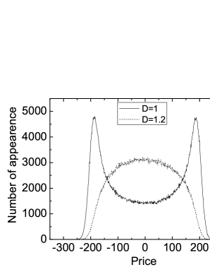
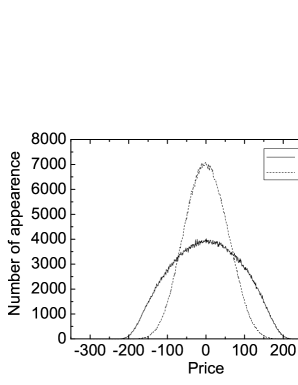
Figure 1: The top curve shows the distribution at low dimensions and illustrates how, as the dimension increases above 1, the bimodal character disappears. The lower curve illustrates how Gaussian behaviour sets in as the dimension goes beyond 2.

Figure 2: Schematic diagram of the change in size of domains for 1 and 2 dimensional networks showing the probability associated with the various different outcomes.

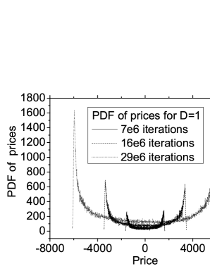
Figure 3: The evolution of PDF in the case of increasing number of iteration.

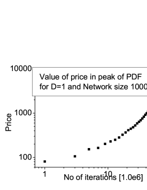
Figure 4: The plot of evolution of peak price with increasing number of iteration.

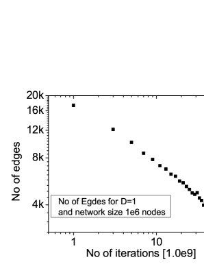
Figure 5: The plot of evolution number of edges (number of domains) with increasing number of iteration.

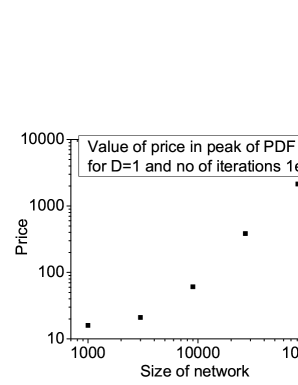
Figure 6: The plot of peak price for different size of the network.

Figure 7: Variance of prices (Risk) as a function of system dimension.

5 Acknowledgment

It is a pleasure for us to dedicate this paper to Prof. Marcel Ausloos and Prof. Dietrich Stauffer on occasions of their 65th birthdays. Authors acknowledge financial support from Polish Ministry of Science and Higher Education, Grant No. 134/E-365/SPB/COST/KN/DWM 105/2005-2007.

References

- [1] K. Sznajd-Weron et al., Opinion evolution in a closed community, Int. J. Mod. Phys. C 11, 2000 1157 arXiv:cond-mat/0101130.
- [2] L Sabatelli and P Richmond Phase transitions, memory and frustration in a Sznajd-like model with synchronous updating International J Mod Phys C 14 2003 1223
- [3] L Sabatelli and P Richmond Non-monotonic spontaneous magnetization in a Sznajd-like Consensus Model Physica A 334 2004 274-280 arXiv:cond-mat/0309375
- [4] Stauffer D, Social applications of two-dimensional Ising models, American Journal of Physics 76, Issue 4, pp. 470-473 .
- [5] L Sabatelli and P Richmond Non-monotonic spontaneous magnetization in a Sznajd-like Consensus Model Physica A 334 2004 274-280 arXiv:cond-mat/0309375
- [6] I. Dornic et al., Critical coarsening without surface tension: the Voter universality class, arXiv:cond-mat/0101202. arXiv:cond-mat/0305015
- [7] L. Frachenbourg et al., Exact results for kinetics of catalytic reactions, Phys. Rev E 53(4), 1995 R3009.