A numerical approach to approximation for a nonlinear ultraparabolic equation

Abstract

In this paper, our aim is to study a numerical method for an ultraparabolic equation with nonlinear source function. Mathematically, the bibliography on initial-boundary value problems for ultraparabolic equations is not extensive although the problems have many applications related to option pricing, multi-parameter Brownian motion, population dynamics and so forth. In this work, we present the approximate solution by virtue of finite difference scheme and Fourier series. For the linear case, we give the approximate solution and obtain a stability result. For the nonlinear case, we use an iterative scheme by linear approximation to get the approximate solution and obtain error estimates. Some numerical examples are given to demonstrate the efficiency of the method.

ifundefinedlettrine ifundefinedshowcaptionsetup

Research

1 Introduction

Let $\mathcal{H}$ be a Hilbert space with the inner product $\left\langle.,.\right\rangle$ and the norm $\left\|.\right\|$. In this paper, we study the following ultraparabolic equation

$$\frac{\partial}{\partial t}u\left(t,s\right)+\frac{\partial}{\partial s}u\left(t,s\right)+\mathcal{L}u\left(t,s\right)=f\left(u\left(t,s\right),t,s\right),\quad\left(t,s\right)\in\left(0,T\right)\times\left(0,T\right),$$ (1)

associated with the initial conditions

$$u\left(0,s\right)=\alpha\left(s\right),\quad u\left(t,0\right)=\beta\left(t\right).$$ (2)

where $\mathcal{L}:\mathcal{D}\left(\mathcal{L}\right)\subset\mathcal{H}\to\mathcal{H}$ is a positive-definite, self-adjoint operator with compact inverse on $\mathcal{H}$ and $\alpha,\beta$ are known smooth functions satisfying $\alpha\left(0\right)=\beta\left(0\right)$ for compatibility at $\left(t,s\right)=\left(0,0\right)$ and $f$ is a nonlinear source function satisfying some conditions which will be fully presented in the next section.

The problem (1)-(2) involving multi-dimensional time variables is called the initial-boundary value problem for ultraparabolic equation. The ultraparabolic equation has many applications in mathematical finance (e.g. [9]), physics (such as multi-parameter Brownian motion [20]) and biological model. Among many applications, the equation (1) arises as a mathematical model of population dynamics, for instance, the dynamics of the age structure of an isolated at the distinct moments of astronomical or biological time and $u\left(t,s\right)$ in this application plays a role as the number of individuals of age $s$ in the population at time $t$. The study of ultraparabolic equation for population dynamics can be found in some papers such as [8, 10]. In particular, Kozhanov [10] studied the existence and uniqueness of regular solutions and its properties for an ultraparabolic model equation in the form of

$$\frac{\partial u}{\partial t}+\frac{\partial u}{\partial s}-\Delta u+h\left(x,t,s\right)u+u\mathcal{A}u=f\left(x,t,s\right),$$

where $\Delta$ is Laplace operator, $\mathcal{A}$ is a nonlocal linear operator. In the same work, the authors Deng and Hallam in [8] considered the age structured population problem formed

$$\frac{\partial u}{\partial t}+\frac{\partial u}{\partial s}-\nabla\cdot\left(k\nabla u-qu\right)=-\mu u,$$

associated with non-locally integro-type initial-bounded conditions.

The ultraparabolic equation is also studied in many other aspects. In the phase of inverse problems, Lorenzi [16] studied the well-posedness of a class of an inverse problem for ultraparabolic partial integrodifferential equations of Volterra type. Very recently, Zouyed and Rebbani [5] proposed the modified quasi-boundary value method to regularize the equation (1) in homogeneous backward case in a class of ill-posed problems. For another studies regarding the properties of solutions of abstract ultraparabolic equations, we can find many papers and some of them are refered to [11, 12, 14, 15, 17, 19].

Even though the numerical method for such a problem is studied long time ago, it is still very limited. We only find some papers, such as [3, 6, 18]. The authors Akrivis, Crouzeix and Thomée [3] investigated a backward Euler scheme and second-order box-type finite difference procedure to numerically approximate the solution to the Dirichlet problem for the ultraparabolic equation (1)-(2) in two different time intervals with the Laplace operator $\mathcal{L}=-\Delta$ and source function $f\equiv 0$. Recently, Ashyralyev and Yilmaz [6] constructed the first and second order difference schemes to approximate the problem (1)-(2) for strongly positive operator and obtained some fundamental stability results. On the other hand, Marcozzi et al. [18] developed an adaptive method-of-lines extrapolation discontinuous Galerkin method for an ultraparabolic model equation given by

$$\frac{\partial u}{\partial t}+a\left(x\right)\frac{\partial u}{\partial s}-\Delta u=f\left(x,t,s\right),$$

with a certain application to the price of an Asian call option.

However, we can see that most of papers for numerical methods aim to study linear cases. Equivalently, numerical methods for nonlinear equations are investigated rarely. Therefore, in this paper we shall study the model problem (1)-(2) in the numerical angle for the smooth solution. From the idea of finite difference scheme and conveying a fundamental result in operator theory, we construct an approximate solution for the nonhomogeneous equation in terms of Fourier series. Combining the same technique and linear approximation, the approximate solution for the nonlinear case is established.

The rest of the paper is organized as follows. In Section 2, we shall consider the linear nonhomogeneous problem (1)-(2) under a result of presentation of discretization solution in multi-dimensional problem. The nonlinear problem is considered in Section 3 and an iterative scheme is showed. Finally, four numerical examples are implemented in Section 4 to verify the effect of the method.

2 The linear nonhomogeneous problem

In this section, we shall introduce the suitable discrete operator used in the time discretization. In order to define the discrete operator involved in the equation in the problem (1)-(2), we consider the multi-dimensional problem given by

$$\left(\sum_{i=1}^{d}\frac{\partial}{\partial t_{i}}\right)u\left(t_{1},t_{2},...,t_{d}\right)+\mathcal{L}u\left(t_{1},t_{2},...,t_{d}\right)=f\left(t_{1},t_{2},...,t_{d}\right),\quad t_{i}\in\left(0,T\right),1\leq i\leq d,$$ (3)

associated with $d$ initial conditions

$$u\left(0,t_{2},...,t_{d}\right)=\alpha_{1}\left(t_{2},t_{3},...,t_{d}\right),...,u\left(t_{1},t_{2},...,0\right)=\alpha_{d}\left(t_{1},t_{2},...,t_{d-1}\right),$$ (4)

for $t_{i}\in\left[0,T\right],1\leq i\leq d$ are $d$ time variables and $d\geq 2$.

Since $\mathcal{L}^{-1}$ is compact, the operator $\mathcal{L}$ admits an orthonormal eigenbasis $\left\{\phi_{n}\right\}_{n\geq 1}$ for $\mathcal{H}$ and eigenvalues $\dfrac{1}{\lambda_{n}}$ of $\mathcal{L}^{-1}$ such that $\mathcal{L}^{-1}\phi_{n}=\dfrac{1}{\lambda_{n}}\phi_{n}$ and $0<\lambda_{1}\leq\lambda_{2}\leq...{\displaystyle\lim_{n\to\infty}\lambda_{n}}=\infty$. Thus, we have from (3) that

$$\left(\sum_{i=1}^{d}\frac{\partial}{\partial t_{i}}\right)\left\langle u\left(t_{1},t_{2},...,t_{d}\right),\phi_{n}\right\rangle+\lambda_{n}\left\langle u\left(t_{1},t_{2},...,t_{d}\right),\phi_{n}\right\rangle=\left\langle f\left(t_{1},t_{2},...,t_{d}\right),\phi_{n}\right\rangle,$$ (5)

and the conditions (4) can be transformed into

$$\left\langle u\left(0,t_{2},...,t_{d}\right),\phi_{n}\right\rangle=\left\langle\alpha_{1}\left(t_{2},t_{3},...,t_{d}\right),\phi_{n}\right\rangle,...,\left\langle u\left(t_{1},t_{2},...,0\right),\phi_{n}\right\rangle=\left\langle\alpha_{d}\left(t_{1},t_{2},...,t_{d-1}\right),\phi_{n}\right\rangle.$$ (6)

By putting

$$u_{n}\left(t_{1},t_{2},...,t_{d}\right)=\left\langle u\left(t_{1},t_{2},...,t_{d}\right),\phi_{n}\right\rangle,\quad f_{n}\left(t_{1},t_{2},...,t_{d}\right)=\left\langle f\left(t_{1},t_{2},...,t_{d}\right),\phi_{n}\right\rangle,$$

$$\alpha_{1,n}\left(t_{2},t_{3},...,t_{d}\right)=\left\langle\alpha_{1}\left(t_{2},t_{3},...,t_{d}\right),\phi_{n}\right\rangle,...,\alpha_{d,n}\left(t_{1},t_{2},...,t_{d-1}\right)=\left\langle\alpha_{d}\left(t_{1},t_{2},...,t_{d-1}\right),\phi_{n}\right\rangle,$$

we shall establish an discrete problem by knowledge of finite difference scheme.

By multiplying both sides of (5) by $\mu_{n}\left(t_{1},t_{2},...,t_{d}\right):=\mbox{exp}\left({\displaystyle\frac{\lambda_{n}}{d}\sum_{i=1}^{d}}t_{i}\right)$, we get

$$\left(\sum_{i=1}^{d}\frac{\partial}{\partial t_{i}}\right)\left(u_{n}\left(t_{1},t_{2},...,t_{d}\right)\mu_{n}\left(t_{1},t_{2},...,t_{d}\right)\right)=f_{n}\left(t_{1},t_{2},...,t_{d}\right)\mu_{n}\left(t_{1},t_{2},...,t_{d}\right).$$

By putting

$$v_{n}\left(t_{1},t_{2},...,t_{d}\right) = u_{n}\left(t_{1},t_{2},...,t_{d}\right)\mu_{n}\left(t_{1},t_{2},...,t_{d}\right)$$

$$F_{n}\left(t_{1},t_{2},...,t_{d}\right) = f_{n}\left(t_{1},t_{2},...,t_{d}\right)\mu_{n}\left(t_{1},t_{2},...,t_{d}\right),$$

we thus have the problem (3)-(4) in a new form.

$$\left(\sum_{i=1}^{d}\frac{\partial}{\partial t_{i}}\right)v_{n}\left(t_{1},t_{2},...,t_{d}\right)=F_{n}\left(t_{1},t_{2},...,t_{d}\right),$$ (7)

associated with the initial conditions

$$v_{n}\left(0,t_{2},...,t_{d}\right) = \beta_{1,n}\left(t_{2},t_{3},...,t_{d}\right):=\alpha_{1,n}\left(t_{2},t_{3},...,t_{d}\right)\mu_{n}\left(0,t_{2},...,t_{d}\right),$$

$$\vdots \vdots \vdots$$

$$v_{n}\left(t_{1},t_{2},...,0\right) = \beta_{d,n}\left(t_{1},t_{2},...,t_{d-1}\right):=\alpha_{d,n}\left(t_{1},t_{2},...,t_{d-1}\right)\mu_{n}\left(t_{1},t_{2},...,0\right).$$ (8)

Then, we treat the transport-shape problem (7)-(8) by finite difference scheme. However, note that standard finite difference scheme may suffer an unstable behaviour in approximate aspect. To avoid the behaviour and lead to our discrete operator, we shall take the equivalent mesh-width in time $\Delta t_{i}=\omega$ for all $1\leq i\leq d$. Also, the source term $f$ in this case is discretized at center nodes to obtain a better order accurate in the first order scheme. They offer stable discretizations of the problem well and then preserve the discrete approach.

For $v_{n}^{k_{1},k_{2},...,k_{d}}:=v_{n}\left(\left(t_{1}\right)_{k_{1}},\left(t_{2}\right)_{k_{2}},...,\left(t_{d}\right)_{k_{d}}\right)$, we get

$$\frac{v_{n}^{k_{1},k_{2},...,k_{d}}-v_{n}^{k_{1}-1,k_{2},...,k_{d}}}{\omega}+\frac{v_{n}^{k_{1}-1,k_{2},...,k_{d}}-v_{n}^{k_{1}-1,k_{2}-1,...,k_{d}}}{\omega}+...$$

$$...+\frac{v_{n}^{k_{1}-1,k_{2}-1,...,k_{d}}-v_{n}^{k_{1}-1,k_{2}-1,...,k_{d}-1}}{\omega}=F_{n}^{k_{1},k_{2},...,k_{d}}$$ (9)

$$F_{n}^{k_{1},k_{2},...,k_{d}}=f_{n}\left(\left(t_{1}\right)_{k_{1}}-\frac{\omega}{2},\left(t_{2}\right)_{k_{2}}-\frac{\omega}{2},...,\left(t_{d}\right)_{k_{d}}-\frac{\omega}{2}\right)\mu_{n}\left(\left(t_{1}\right)_{k_{1}},\left(t_{2}\right)_{k_{2}},...,\left(t_{d}\right)_{k_{d}}\right),$$

for $1\leq k_{i}\leq M,1\leq i\leq d$,

$$v_{n}^{0,k_{2},...,k_{d}} = \beta_{1,n}^{k_{2},k_{3},...,k_{d}}:=\alpha_{1,n}\left(\left(t_{2}\right)_{k_{2}},\left(t_{3}\right)_{k_{3}},...,\left(t_{d}\right)_{k_{d}}\right)\mu_{n}\left(0,\left(t_{2}\right)_{k_{2}},...,\left(t_{d}\right)_{k_{d}}\right)$$

$$\vdots \vdots \vdots$$

$$v_{n}^{k_{1},k_{2},...,0} = \beta_{d,n}^{k_{1},k_{2},...,k_{d-1}}:=\alpha_{d,n}\left(\left(t_{1}\right)_{k_{1}},\left(t_{2}\right)_{k_{2}},...,\left(t_{d-1}\right)_{k_{d-1}}\right)\mu_{n}\left(\left(t_{1}\right)_{k_{1}},\left(t_{2}\right)_{k_{2}},...,0\right),$$

for $0\leq k_{i}\leq M$ and where $\left(t_{i}\right)_{k_{i}}=k_{i}\omega,1\leq i\leq d$ and $M\omega=T$.

By simple calculation, it follows from (9) that the local discrete operator is

$$v_{n}^{k_{1},k_{2},...,k_{d}}=\omega F_{n}^{k_{1},k_{2},...,k_{d}}+v_{n}^{k_{1}-1,k_{2}-1,...,k_{d}-1}.$$ (11)

Lemma 0.1.

For every $n\in\mathbb{N}$, if $v_{n}^{k_{1},k_{2},...,k_{d}}$ satisfies (11) for all $k_{i}\in\left[1,M\right],1\leq i\leq d$, then one has

$$v_{n}^{k_{1},k_{2},...,k_{d}}=\omega\sum_{l=1}^{p}F_{n}^{k_{1}-p+l,k_{2}-p+l,...,k_{d}-p+l}+v_{n}^{k_{1}-p,k_{2}-p,...,k_{d}-p},$$ (12)

for all $p\in\mathbb{N}$.

Proof.

We shall prove (12) by induction. We can see that it holds for $p=1$.

For $p=2$, we have

$$v_{n}^{k_{1},k_{2},...,k_{d}} = \omega F_{n}^{k_{1},k_{2},...,k_{d}}+\omega f_{n}^{k_{1}-1,k_{2}-1,...,k_{d}-1}+v_{n}^{k_{1}-2,k_{2}-2,...,k_{d}-2}$$

$$= \omega F_{n}^{k_{1},k_{2},...,k_{d}}+v_{n}^{k_{1}-1,k_{2}-1,...,k_{d}-1}.$$

Thus, (12) holds for $p=2$.

Now, we assume that (12) holds for $p=r$. It means that

$$v_{n}^{k_{1},k_{2},...,k_{d}}=\omega\sum_{l=1}^{r}F_{n}^{k_{1}-r+l,k_{2}-r+l,...,k_{d}-r+l}+v_{n}^{k_{1}-r,k_{2}-r,...,k_{d}-r}.$$

We shall prove that it aslo holds for $p=r+1$. Indeed, we get

$$v_{n}^{k_{1},k_{2},...,k_{d}} = \omega\sum_{l=1}^{r}F_{n}^{k_{1}-r+l,k_{2}-r+l,...,k_{d}-r+l}$$

$$+\omega F_{n}^{k_{1}-r,k_{2}-r,...,k_{d}-r}+v_{n}^{k_{1}-r-1,k_{2}-r-1,...,k_{d}-r-1}$$

$$= \omega\sum_{l=1}^{r+1}F_{n}^{k_{1}-r-1+l,k_{2}-r-1+l,...,k_{d}-r-1+l}+v_{n}^{k_{1}-r-1,k_{2}-r-1,...,k_{d}-r-1}.$$

Therefore, (12) holds for $p=r+1$. By induction, we completely finish the proof. ∎

From (12), we shall obtain the discrete solution by Fourier series. It should be stated that the discrete solution is, in multi-dimensional, involved by many situations according to the set $\mathcal{E}_{d}=\left\{k_{1},k_{2},...,k_{d}\right\}$, more exactly $d!$ situations. As introduced, in this paper we aim to consider the ultraparabolic problem with two time dimension since there are many studies on this problem in real application. Hence, the solution of the discrete problem of (1)-(2) in linear nonhomogeneous case is

$$v_{n}^{k_{1},k_{2}}=\omega\sum_{l=1}^{p}F_{n}^{k_{1}-p+l,k_{2}-p+l}+v_{n}^{k_{1}-p,k_{2}-p},$$

and its explicit form is given as follows.

If $k_{1}>k_{2}$, we replace $p$ by $k_{2}$ to get

$$v_{n}^{k_{1},k_{2}} = \omega\sum_{l=1}^{k_{2}}F_{n}^{k_{1}-k_{2}+l,l}+v_{n}^{k_{1}-k_{2},0}$$ (13)

$$= \omega\sum_{l=1}^{k_{2}}F_{n}^{k_{1}-k_{2}+l,l}+\beta_{n}^{k_{1}-k_{2}}\mu_{n}^{k_{1}-k_{2},0}.$$

Similarly, for $k_{2}>k_{1}$ we replace $p$ by $k_{1}$ to obtain

$$v_{n}^{k_{1},k_{2}}=\omega\sum_{l=1}^{k_{1}}F_{n}^{l,k_{2}-k_{1}+l}+\alpha_{n}^{k_{2}-k_{1}}\mu_{n}^{0,k_{2}-k_{1}}.$$ (14)

From (13)-(14), we conclude the discrete solution for the two-time-variable ultraparabolic (1)-(2) in linear nonhomogeneous case is

$$u^{k_{1},k_{2}} = \sum_{n=1}^{\infty}v_{n}^{k_{1},k_{2}}\left(\mu_{n}^{k_{1},k_{2}}\right)^{-1}\phi_{n}$$ (15)

$$= \begin{cases}\sum_{n=1}^{\infty}\omega\sum_{l=1}^{k_{2}}\mu_{n}^{k_{1}-k_{2}+l,l}\left(\mu_{n}^{k_{1},k_{2}}\right)^{-1}f_{n}^{k_{1}-k_{2}+l,l}\phi_{n}\\ +\sum_{n=1}^{\infty}\left(\mu_{n}^{k_{1},k_{2}}\right)^{-1}\beta_{n}^{k_{1}-k_{2}}\mu_{n}^{k_{1}-k_{2},0}\phi_{n}&,k_{1}>k_{2},\\ \sum_{n=1}^{\infty}\omega\sum_{l=1}^{k_{1}}\mu_{n}^{l,k_{2}-k_{1}+l}\left(\mu_{n}^{k_{1},k_{2}}\right)^{-1}f_{n}^{l,k_{2}-k_{1}+l}\phi_{n}\\ +\sum_{n=1}^{\infty}\left(\mu_{n}^{k_{1},k_{2}}\right)^{-1}\alpha_{n}^{k_{2}-k_{1}}\mu_{n}^{0,k_{2}-k_{1}}\phi_{n}&,k_{2}>k_{1}.\end{cases}$$

Furthermore, we obtain a stability result in the following theorem.

Theorem 0.2.

Let $u^{k_{1},k_{2}}$ in (15) be the discrete solution of the problem (1)-(2) in linear nonhomogeneous case, then there exists a positive constant $C_{T}$ independent of $k_{1},k_{2}$ and $\omega$ such that

$$\sup_{1\leq k_{1},k_{2}\leq M}\left\|u^{k_{1},k_{2}}\right\|^{2}\leq C_{T}\left(\sup_{1\leq k_{1},k_{2}\leq M}\left\|f^{k_{1},k_{2}}\right\|^{2}+\sup_{0\leq k_{1}\leq M}\left\|\alpha^{k_{2}}\right\|^{2}+\sup_{0\leq k_{1}\leq M}\left\|\beta^{k_{1}}\right\|^{2}\right).$$

Proof.

Since $\mu_{n}^{k_{1}-k_{2}+l,l}\leq\mu_{n}^{k_{1},k_{2}}$ and $\mu_{n}^{k_{1}-k_{2},0}\leq\mu_{n}^{k_{1},k_{2}}$, by using Parseval’s identity we have

$$\left\|u^{k_{1},k_{2}}\right\|^{2} = \sum_{n=1}^{\infty}\left|v_{n}^{k_{1},k_{2}}\left(\mu_{n}^{k_{1},k_{2}}\right)^{-1}\right|^{2}$$ (16)

$$\leq 2\omega^{2}\sum_{n=1}^{\infty}\left|\sum_{l=1}^{k_{2}}\mu_{n}^{k_{1}-k_{2}+l,l}\left(\mu_{n}^{k_{1},k_{2}}\right)^{-1}f_{n}^{k_{1}-k_{2}+l,l}\right|^{2}$$

$$+2\sum_{n=1}^{\infty}\left|\left(\mu_{n}^{k_{1},k_{2}}\right)^{-1}\mu_{n}^{k_{1}-k_{2},0}\beta_{n}^{k_{1}-k_{2}}\right|^{2}$$

$$\leq 2k_{2}^{2}\omega^{2}\sup_{1\leq k_{1},k_{2}\leq M}\sum_{n=1}^{\infty}\left|f_{n}^{k_{1},k_{2}}\right|^{2}+2\sum_{n=1}^{\infty}\left|\beta_{n}^{k_{1}-k_{2}}\right|^{2}$$

$$\leq 2T^{2}\sup_{1\leq k_{1},k_{2}\leq M}\left\|f^{k_{1},k_{2}}\right\|^{2}+2\left\|\beta^{k_{1}-k_{2}}\right\|^{2}$$

$$\leq C_{T}\left(\sup_{1\leq k_{1},k_{2}\leq M}\left\|f^{k_{1},k_{2}}\right\|^{2}+\sup_{0\leq k_{1}\leq M}\left\|\beta^{k_{1}}\right\|^{2}\right),$$

for $k_{1}>k_{2}$.

Similarly, for $k_{2}>k_{1}$ we also have

$$\left\|u^{k_{1},k_{2}}\right\|^{2} \leq 2T^{2}\sup_{1\leq k_{1},k_{2}\leq M}\left\|f^{k_{1},k_{2}}\right\|^{2}+2\left\|\alpha^{k_{2}-k_{1}}\right\|^{2}$$ (17)

$$\leq C_{T}\left(\sup_{1\leq k_{1},k_{2}\leq M}\left\|f^{k_{1},k_{2}}\right\|^{2}+\sup_{0\leq k_{2}\leq M}\left\|\alpha^{k_{2}}\right\|^{2}\right).$$

Combining (16) and (17), we conclude that

$$\sup_{1\leq k_{1},k_{2}\leq M}\left\|u^{k_{1},k_{2}}\right\|^{2}\leq C_{T}\left(\sup_{1\leq k_{1},k_{2}\leq M}\left\|f^{k_{1},k_{2}}\right\|^{2}+\sup_{0\leq k_{2}\leq M}\left\|\alpha^{k_{2}}\right\|^{2}+\sup_{0\leq k_{1}\leq M}\left\|\beta^{k_{1}}\right\|^{2}\right),$$

which gives the desired result.∎

Remark 0.3.

The stability result for the ultraparabolic problem in multi-time dimension (9)-(LABEL:eq:10) can be obtained in the same way according to the situations the discrete solution has. Particularly, one has

$$\sup_{1\leq k_{i}\leq M,1\leq i\leq d}\left\|u^{k_{1},k_{2},...,k_{d}}\right\|^{2}\leq C_{T}\left(\sup_{1\leq k_{i}\leq M,1\leq i\leq d}\left\|f^{k_{1},k_{2},...,k_{d}}\right\|^{2}+\sum_{j=1}^{d}\sup_{0\leq k_{i}\leq M,1\leq i\leq d}\left\|\alpha_{j}^{k_{i}}\right\|^{2}\right).$$

3 The nonlinear problem

Until now, numerical methods for nonlinear ultraparabolic equations are still very rare. From that point, we begin the section by considering the ultraparabolic problem (1)-(2) with the nonlinear function $f$ satisfying Lipschitz condition. By simple calculation analogous to the steps in linear nonhomogeneous case, we get the discrete solution, then use linear approximation to get the explicit form of the approximate solution. Particularly, the following problem is considered.

$$\left(P\right):\quad\begin{cases}\frac{\partial}{\partial t}u\left(t,s\right)+\frac{\partial}{\partial s}u\left(t,s\right)+\mathcal{L}u\left(t,s\right)=f\left(u\left(t,s\right),t,s\right),\\ u\left(0,s\right)=\alpha\left(s\right),\quad u\left(t,0\right)=\beta\left(t\right),\end{cases}$$

for the nonlinear source function $f$ satisfying the Lipschitz condition:

$$\left\|f\left(u,t,s\right)-f\left(v,t,s\right)\right\|\leq K\left\|u-v\right\|,$$ (18)

where $K$ is a positive number independent of $u,v,t,s$.

On account of the orthonormal basis $\left\{\phi_{n}\right\}_{n\geq 1}$ admitted by $\mathcal{L}$ and corresponding eigenvalues $\lambda_{n}$, the problem $\left(P\right)$ can be made in the following manner.

$$\begin{cases}\frac{\partial}{\partial t}\left\langle u\left(t,s\right),\phi_{n}\right\rangle+\frac{\partial}{\partial s}\left\langle u\left(t,s\right),\phi_{n}\right\rangle+\lambda_{n}\left\langle u\left(t,s\right),\phi_{n}\right\rangle=\left\langle f\left(u\left(t,s\right),t,s\right),\phi_{n}\right\rangle,\\ \left\langle u\left(0,s\right),\phi_{n}\right\rangle=\left\langle\alpha\left(s\right),\phi_{n}\right\rangle,\quad\left\langle u\left(t,0\right),\phi_{n}\right\rangle=\left\langle\beta\left(t\right),\phi_{n}\right\rangle.\end{cases}$$ (19)

With $\mu_{n}\left(t,s\right)=\mbox{exp}\left(\dfrac{\lambda_{n}}{2}\left(t+s\right)\right)$, the problem (19) is equivalent to the following problem.

$$\begin{cases}\left(\frac{\partial}{\partial t}+\frac{\partial}{\partial s}\right)\left(\left\langle u\left(t,s\right),\phi_{n}\right\rangle\mu_{n}\left(t,s\right)\right)=\left\langle f\left(u\left(t,s\right),t,s\right),\phi_{n}\right\rangle\mu_{n}\left(t,s\right),\\ \left\langle u\left(0,s\right),\phi_{n}\right\rangle\mu_{n}\left(t,s\right)=\left\langle\alpha\left(s\right),\phi_{n}\right\rangle\mu_{n}\left(t,s\right),\\ \left\langle u\left(t,0\right),\phi_{n}\right\rangle\mu_{n}\left(t,s\right)=\left\langle\beta\left(t\right),\phi_{n}\right\rangle\mu_{n}\left(t,s\right).\end{cases}$$ (20)

For the numerical solution of this problem by finite difference scheme as introduced in the above section, a uniform grid of mesh-points $\left(t,s\right)=\left(t_{k},s_{m}\right)$ is showed. Here $t_{k}=k\omega$ and $s_{m}=m\omega$, where $k$ and $m$ are integers and $\omega$ the equivalent mesh-width in time $t$ and $s$. We shall seek an discrete solution $u^{k,m}=u\left(t_{k},s_{m}\right)$ determined by an equation obtained by replacing the time derivatives in (20) by difference quotients. The equation in (20) becomes

$$\frac{\left\langle u^{k,m},\phi_{n}\right\rangle\mu_{n}^{k,m}-\left\langle u^{k-1,m},\phi_{n}\right\rangle\mu_{n}^{k-1,m}}{\omega}+\frac{\left\langle u^{k-1,m},\phi_{n}\right\rangle\mu_{n}^{k-1,m}-\left\langle u^{k-1,m-1},\phi_{n}\right\rangle\mu_{n}^{k-1,m-1}}{\omega}$$

$$=\left\langle f\left(u^{k,m},t_{k},s_{m}\right),\phi_{n}\right\rangle\mu_{n}^{k,m},$$

(21)

and the initial conditions are

$$\left\langle u\left(0,s_{m}\right),\phi_{n}\right\rangle\mu_{n}^{k,m}=\left\langle\alpha^{m},\phi_{n}\right\rangle\mu_{n}^{k,m},\quad\left\langle u\left(t_{k},0\right),\phi_{n}\right\rangle\mu_{n}^{k,m}=\left\langle\beta^{k},\phi_{n}\right\rangle\mu_{n}^{k,m},$$

where $\mu_{n}^{k,m}=\mu_{n}\left(t_{k},s_{m}\right),\alpha^{m}=\alpha\left(s_{m}\right)$ and $\beta^{k}=\beta\left(t_{k}\right)$.

By induction, it follows from (21) that

$$\left\langle u^{k,m},\phi_{n}\right\rangle\mu_{n}^{k,m} = \omega\sum_{l=1}^{p}\left\langle f\left(u^{k-p+l,m-p+l},t_{k-p+l},s_{m-p+l}\right),\phi_{n}\right\rangle\mu_{n}^{k-p+l,m-p+l}$$

$$+\left\langle u^{k-p,m-p},\phi_{n}\right\rangle\mu_{n}^{k-p,m-p},$$

for all $p\in\mathbb{N}$.

Thus, the explicit form of discrete solution of $\left(P\right)$ is obtained.

$$u^{k,m}=\begin{cases}\sum_{n=1}^{\infty}\omega\sum_{l=1}^{m}\mu_{n}^{k-m+l,l}\left(\mu_{n}^{k,m}\right)^{-1}\left\langle f\left(u^{k-m+l,l},t_{k-m+l},s_{l}\right),\phi_{n}\right\rangle\phi_{n}\\ +\sum_{n=1}^{\infty}\left(\mu_{n}^{k,m}\right)^{-1}\left\langle\beta^{k-m},\phi_{n}\right\rangle\mu_{n}^{k-m,0}\phi_{n}&,k>m,\\ \sum_{n=1}^{\infty}\omega\sum_{l=1}^{m}\mu_{n}^{l,m-k+l}\left(\mu_{n}^{k,m}\right)^{-1}\left\langle f\left(u^{l,m-k+l},t_{l},s_{m-k+l}\right),\phi_{n}\right\rangle\phi_{n}\\ +\sum_{n=1}^{\infty}\left(\mu_{n}^{k,m}\right)^{-1}\left\langle\alpha^{m-k},\phi_{n}\right\rangle\mu_{n}^{0,m-k}\phi_{n}&,m>k.\end{cases}$$ (22)

From now on, we shall give an iterative scheme by knowledge of linear approximation.

Choosing $u_{0}^{k,m}=0$, we seek $u_{q}^{k,m},q\geq 1$ satisfying

$$u_{q}^{k,m}=\begin{cases}\sum_{n=1}^{\infty}\omega\sum_{l=1}^{m}\mu_{n}^{k-m+l,l}\left(\mu_{n}^{k,m}\right)^{-1}\left\langle f\left(u_{q-1}^{k-m+l,l},t_{k-m+l},s_{l}\right),\phi_{n}\right\rangle\phi_{n}\\ +\sum_{n=1}^{\infty}\left(\mu_{n}^{k,m}\right)^{-1}\left\langle\beta^{k-m},\phi_{n}\right\rangle\mu_{n}^{k-m,0}\phi_{n}&,k>m,\\ \sum_{n=1}^{\infty}\omega\sum_{l=1}^{k_{1}}\mu_{n}^{l,m-k+l}\left(\mu_{n}^{k,m}\right)^{-1}\left\langle f\left(u_{q-1}^{l,m-k+l},t_{l},s_{m-k+l}\right),\phi_{n}\right\rangle\phi_{n}\\ +\sum_{n=1}^{\infty}\left(\mu_{n}^{k,m}\right)^{-1}\left\langle\alpha^{m-k},\phi_{n}\right\rangle\mu_{n}^{0,m-k}\phi_{n}&,m>k.\end{cases}$$ (23)

Here $u_{q}^{k,m}$ is called the approximate solution for the problem (1)-(2). Our results are to prove that this solution approach to the discrete solution $u^{k,m}$ in norm $\mathcal{H}$ as $q\to\infty$ and study the stability estimate of $u_{q}^{k,m}$ in norm $\mathcal{H}$ with respect to the initial data and the right hand side $f\left(u_{q-1}\right)$.

Theorem 0.4.

Let $\left\{u_{q}^{k,m}\right\}_{q\geq 1}$ be the iterative sequence defined by (23). Then, it satisfies the a priori estimate

$$\sup_{1\leq k,m\leq M}\left\|u_{q}^{k,m}\right\|^{2}\leq C_{T}\left(\sup_{1\leq k,m\leq M}\left\|u_{q-1}^{k,m}\right\|^{2}+\sup_{1\leq k,m\leq M}\left\|f\left(0,t_{k},s_{m}\right)\right\|^{2}+\sup_{0\leq m\leq M}\left\|\alpha^{m}\right\|^{2}+\sup_{0\leq k\leq M}\left\|\beta^{k}\right\|^{2}\right),$$

where $C_{T}$ is a positive constant depending only on $T$.

Theorem 0.5.

If the nonlinear source function $f$ of the problem $\left(P\right)$ satisfying the Lipschitz condition (18). Then, the iterative sequence $\left\{u_{q}^{k,m}\right\}$ defined by (23) strongly converges to the discrete solution $u^{k,m}$ (22) of $\left(P\right)$ in norm $\mathcal{H}$ in the sense of

$$\sup_{1\leq k,m\leq M}\left\|u_{q}^{k,m}-u^{k,m}\right\|\leq\frac{\kappa_{T}^{q}}{1-\kappa_{T}}\sup_{1\leq k,m\leq M}\left\|u_{1}^{k,m}\right\|,$$

where $\kappa_{T}<1$ is a positive constant depending only on $T$.

The problem (1)-(2) with the nonlinear function $f$ in a bit larger class in terms of non-Lipschitz functions can be solved in the similar way. Specifically, the function $f$ will be defined by the product of two functions $g$ and $h$. We also study the a priori estimate of solution and obtain convergence rate between the approximate solution $u_{q}^{k,m}$ and the discrete solution $u^{k,m}$. This study continuously contributes to the state of rarity of numerical methods for the nonlinear ultraparabolic problems. In particular, we shall consider the following problem.

$$\left(Q\right):\quad\begin{cases}\frac{\partial}{\partial t}u\left(t,s\right)+\frac{\partial}{\partial s}u\left(t,s\right)+\mathcal{L}u\left(t,s\right)=g\left(u\left(t,s\right),t,s\right)h\left(u\left(t,s\right),t,s\right),\\ u\left(0,s\right)=\alpha\left(s\right),\quad u\left(t,0\right)=\beta\left(t\right),\end{cases}$$

for $g$ and $h$ satisfying the following conditions.

$$g\left(u,t,s\right)\leq K_{1},\quad\left\|h\left(u,t,s\right)-h\left(v,t,s\right)\right\|\leq K_{2}\left\|u-v\right\|,$$ (24)

where $K_{1},K_{2}$ are positive constants independent of $u,v,t,s$.

Similar to the problem $\left(P\right)$, the approximate solution $u_{q}^{k,m}$ of $\left(Q\right)$ is given by

$$u_{q}^{k,m}=\begin{cases}\sum_{n=1}^{\infty}\omega\sum_{l=1}^{m}\mu_{n}^{k-m+l,l}\left(\mu_{n}^{k,m}\right)^{-1}\left\langle\left(gh\right)\left(u_{q-1}^{k-m+l,l},t_{k-m+l},s_{l}\right),\phi_{n}\right\rangle\phi_{n}\\ +\sum_{n=1}^{\infty}\left(\mu_{n}^{k,m}\right)^{-1}\left\langle\beta^{k-m},\phi_{n}\right\rangle\mu_{n}^{k-m,0}\phi_{n}&,k>m,\\ \sum_{n=1}^{\infty}\omega\sum_{l=1}^{k_{1}}\mu_{n}^{l,m-k+l}\left(\mu_{n}^{k,m}\right)^{-1}\left\langle\left(gh\right)\left(u_{q-1}^{l,m-k+l},t_{l},s_{m-k+l}\right),\phi_{n}\right\rangle\phi_{n}\\ +\sum_{n=1}^{\infty}\left(\mu_{n}^{k,m}\right)^{-1}\left\langle\alpha^{m-k},\phi_{n}\right\rangle\mu_{n}^{0,m-k}\phi_{n}&,m>k.\end{cases}$$ (25)

Theorem 0.6.

Let $\left\{u_{q}^{k,m}\right\}_{q\geq 1}$ be the iterative sequence defined by (25). Then, it satisfies the a priori estimate

$$\sup_{1\leq k,m\leq M}\left\|u_{q}^{k,m}\right\|^{2}\leq C_{T}\left(\sup_{1\leq k,m\leq M}\left\|u_{q-1}^{k,m}\right\|^{2}+\sup_{1\leq k,m\leq M}\left\|h\left(0,t_{k},s_{m}\right)\right\|^{2}+\sup_{0\leq m\leq M}\left\|\alpha^{m}\right\|^{2}+\sup_{0\leq k\leq M}\left\|\beta^{k}\right\|^{2}\right),$$

where $C_{T}$ is a positive constant depending only on $T$.

Theorem 0.7.

If the nonlinear source function $f=gh$ of the problem $\left(Q\right)$ satisfying the conditions (24), then the iterative sequence $\left\{u_{q}^{k,m}\right\}$ defined in (25) strongly converges to the discrete solution $u^{k,m}$ (22) of $\left(Q\right)$ in norm $\mathcal{H}$ in the sense of

$$\left\|u_{q}^{k,m}-u^{k,m}\right\|\leq\kappa_{T}^{q}\sup_{1\leq k,m\leq M}\left\|u_{1}^{k,m}\right\|,$$

where $\kappa_{T}<1$ is a postive constant depending only on $T$.

Remark 0.8.

Assume that $u_{ex}^{k,m}$ is the exact solution of the problem $\left(P\right)$ (also $\left(Q\right)$) at $\left(t_{k},s_{m}\right)$. By finite difference scheme, we know that the error between the exact solution $u_{ex}^{k,m}$ and discrete solution $u^{k,m}$ is of order $\mathcal{O}\left(\omega\right)$. Therefore, by triangle inequality, the error estimate between the exact solution and approximate solution $u_{q}^{k,m}$ is

$$\sup_{1\leq k,m\leq M}\left\|u_{ex}^{k,m}-u_{q}^{k,m}\right\|\leq C\left(\omega+\kappa_{T}^{q}\right),$$

for the problem $\left(P\right)$ (also $\left(Q\right)$) where $C$ is a positive constant independent of $\omega,\kappa_{T}$ and $q$, provided by the smoothness of the exact function.

Proof of Theorem 4.

Proof.

Using Parseval’s identity in (23) for the case $k>m$, we have

$$\left\|u_{q}^{k,m}\right\|^{2} \leq 2\omega^{2}\sum_{n=1}^{\infty}\left|\sum_{l=1}^{m}\mu_{n}^{k-m+l,l}\left(\mu_{n}^{k,m}\right)^{-1}\left\langle f\left(u_{q-1}^{k-m+l,l},t_{k-m+l},s_{l}\right),\phi_{n}\right\rangle\right|^{2}$$ (26)

$$+2\sum_{n=1}^{\infty}\left|\mu_{n}^{k-m,0}\left(\mu_{n}^{k,m}\right)^{-1}\left\langle\beta^{k-m},\phi_{n}\right\rangle\right|^{2}$$

$$\leq 2\omega^{2}m^{2}\sup_{1\leq k,m\leq M}\sum_{n=1}^{\infty}\left|\left\langle f\left(u_{q-1}^{k,m},t_{k},s_{m}\right),\phi_{n}\right\rangle\right|^{2}$$

$$+2\sup_{0\leq k\leq M}\sum_{n=1}^{\infty}\left|\left\langle\beta^{k},\phi_{n}\right\rangle\right|^{2}$$

$$\leq 2T^{2}\sup_{1\leq k,m\leq M}\left\|f\left(u_{q-1}^{k,m},t_{k},s_{m}\right)\right\|^{2}+2\sup_{0\leq k\leq M}\left\|\beta^{k}\right\|^{2}.$$

Similarly, we can deduce for the case $k<m$ that

$$\left\|u_{q}^{k,m}\right\|^{2}\leq 2T^{2}\sup_{1\leq k,m\leq M}\left\|f\left(u_{q-1}^{k,m},t_{k},s_{m}\right)\right\|^{2}+2\sup_{0\leq m\leq M}\left\|\alpha^{m}\right\|^{2}.$$ (27)

Moreover, from the condition (18), we have

$$\left\|f\left(u_{q-1}^{k,m},t_{k},s_{m}\right)\right\| \leq \left\|f\left(u_{q-1}^{k,m},t_{k},s_{m}\right)-f\left(u_{0}^{k,m},t_{k},s_{m}\right)\right\|+\left\|f\left(u_{0}^{k,m},t_{k},s_{m}\right)\right\|$$ (28)

$$\leq K\left\|u_{q-1}^{k,m}\right\|+\left\|f\left(0,t_{k},s_{m}\right)\right\|.$$

Combining (26)-(28) and putting $C_{T}=\max\left\{2T^{2}\left(K^{2}+1\right);2\right\}$, we get

$$\sup_{1\leq k,m\leq M}\left\|u_{q}^{k,m}\right\|^{2} \leq 2T^{2}\left(K^{2}+1\right)\left(\sup_{1\leq k,m\leq M}\left\|u_{q-1}^{k,m}\right\|^{2}+\sup_{1\leq k,m\leq M}\left\|f\left(0,t_{k},s_{m}\right)\right\|^{2}\right)$$

$$+2\left(\sup_{0\leq m\leq M}\left\|\alpha^{m}\right\|^{2}+\sup_{0\leq k\leq M}\left\|\beta^{k}\right\|^{2}\right)$$

$$\leq C_{T}\left(\sup_{1\leq k,m\leq M}\left\|u_{q-1}^{k,m}\right\|^{2}+\sup_{1\leq k,m\leq M}\left\|f\left(0,t_{k},s_{m}\right)\right\|^{2}\right.$$

$$\left.+\sup_{0\leq m\leq M}\left\|\alpha^{m}\right\|^{2}+\sup_{0\leq k\leq M}\left\|\beta^{k}\right\|^{2}\right).$$

∎

Proof of Theorem 5.

Proof.

For short, we denote $f^{k,m}\left(u^{k,m}\right)=f\left(u^{k,m},t_{k},s_{m}\right)$. Putting $w_{q}^{k,m}=u_{q+1}^{k,m}-u_{q}^{k,m}$, it follows from (23) that for $k>m$ we have

$$\left\|w_{q}^{k,m}\right\|^{2} \leq \omega^{2}\sum_{n=1}^{\infty}\left|\sum_{l=1}^{m}\left\langle f^{k-m+l,l}\left(u_{q}^{k-m+l,l}\right)-f^{k-m+l,l}\left(u_{q-1}^{k-m+l,l}\right),\phi_{n}\right\rangle\right|^{2}$$

$$\leq \omega^{2}m^{2}\sup_{1\leq k,m\leq M}\left\|f^{k,m}\left(u_{q}^{k,m}\right)-f^{k,m}\left(u_{q-1}^{k,m}\right)\right\|^{2}$$

$$\leq T^{2}K^{2}\sup_{1\leq k,m\leq M}\left\|u_{q}^{k,m}-u_{q-1}^{k,m}\right\|^{2}.$$

Thus, we get

$$\left\|w_{q}^{k,m}\right\|\leq TK\sup_{1\leq k,m\leq M}\left\|w_{q-1}^{k,m}\right\|.$$

We can always choose $T>0$ small enough such that $\kappa_{T}:=TK<1$. Then, we have

$$\left\|u_{q+r}^{k,m}-u_{q}^{k,m}\right\| \leq \left\|u_{q+r}^{k,m}-u_{q+r-1}^{k,m}\right\|+...+\left\|u_{q+1}^{k,m}-u_{q}^{k,m}\right\|$$

$$\leq \kappa_{T}^{q+r-1}\sup_{1\leq k,m\leq M}\left\|u_{1}^{k,m}-u_{0}^{k,m}\right\|+...+\kappa_{T}^{q}\sup_{1\leq k,m\leq M}\left\|u_{1}^{k,m}-u_{0}^{k,m}\right\|$$

$$\leq \kappa_{T}^{q}\left(\kappa_{T}^{r-1}+\kappa_{T}^{r-2}+...+1\right)\sup_{1\leq k,m\leq M}\left\|u_{1}^{k,m}\right\|$$

$$\leq \frac{\kappa_{T}^{q}\left(1-\kappa_{T}^{r}\right)}{1-\kappa_{T}}\sup_{1\leq k,m\leq M}\left\|u_{1}^{k,m}\right\|.$$

Therefore, we obtain

$$\left\|u_{q+r}^{k,m}-u_{q}^{k,m}\right\|\leq\frac{\kappa_{T}^{q}}{1-\kappa_{T}}\sup_{1\leq k,m\leq M}\left\|u_{1}^{k,m}\right\|,$$ (29)

which leads to the claim that $\left\{u_{q}^{k,m}\right\}$ is a Cauchy sequence in $\mathcal{H}$ and then, there exists uniquely $u^{k,m}\in\mathcal{H}$ such that $u_{q}^{k,m}\to u^{k,m}$ as $q\to\infty$. Because of this convergence and Lipschitz property (18) of nonlinear source term $f$, it is easy to prove that $f\left(u_{q}^{k,m}\right)\to f\left(u^{k,m}\right)$ as $q\to\infty$. Therefore, $u^{k,m}$ is the discrete solution of the problem $\left(P\right)$.

When $r\to\infty$, it follows (29) from that

$$\left\|u^{k,m}-u_{q}^{k,m}\right\|\leq\frac{\kappa_{T}^{q}}{1-\kappa_{T}}\sup_{1\leq k,m\leq M}\left\|u_{1}^{k,m}\right\|.$$

For $m>k$, we also have a similar proof. Hence, we complete the proof of the theorem. ∎

4 Numerical examples

In this section, we are going to show four numerical examples in order to validate the efficiency of our scheme. It will be observed by comparing the results between numerical and exact solutions. We shall choose given functions in such a way that they lead to a given exact solution. In details, we have four examples implementing all considered cases. The first and second examples are of the linear nonhomogeneous case while the rest of examples are showed for nonlinear cases $f=\sin\left(u\right)$ and $f=u\sin\left(\dfrac{u}{2}\right)$ implying Lipschitz and non-Lipschitz functions. The examples are involved with the Hilbert space $\mathcal{H}=L^{2}\left(0,\pi\right)$ and associated with homogeneous boundary conditions. On the other hand, numerical results with many 3-D graphs shall be discussed in the last subsection.

4.1 Example 1

We consider the problem

$$\begin{cases}u_{t}\left(x,t,s\right)+u_{s}\left(x,t,s\right)-u_{xx}\left(x,t,s\right)=f\left(x,t,s\right)&,\left(x,t,s\right)\in\left(0,\pi\right)\times\left(0,1\right)\times\left(0,1\right),\\ u\left(0,t,s\right)=u\left(\pi,t,s\right)=0&,\left(t,s\right)\in\left[0,1\right]\times\left[0,1\right],\\ u\left(x,0,s\right)=\alpha\left(x,s\right)&,\left(x,s\right)\in\left[0,\pi\right]\times\left[0,1\right],\\ u\left(x,t,0\right)=\beta\left(x,t\right)&,\left(x,t\right)\in\left[0,\pi\right]\times\left[0,1\right],\end{cases}$$

where $f\left(x,t,s\right)=-2e^{-2t-s}\sin x,\alpha\left(x,s\right)=e^{-s}\sin x$ and $\beta\left(x,t\right)=e^{-2t}\sin x$.

In this example, we see that $\mathcal{D}\left(\mathcal{L}\right)=H_{0}^{1}\left(0,\pi\right)\cap H^{2}\left(0,\pi\right)$, then we get an orthonormal eigenbasis $\phi_{n}\left(x\right)=\sqrt{\dfrac{2}{\pi}}\sin\left(\sqrt{\lambda_{n}}x\right)$ where the eigenvalues $\lambda_{n}=n^{2}$. Therefore, by time discretization $t_{k}=k\omega,s_{m}=m\omega$ and $\omega=\dfrac{1}{M}$ the approximate solution (15) is

$$u\left(x,t_{k},s_{m}\right)=\frac{-2\omega}{e^{\frac{1}{2}\left(t_{k}+s_{m}\right)}}\sum_{l=1}^{m}e^{-\frac{1}{2}\left(3t_{k-m+l}+s_{l}\right)+\frac{3}{2}\omega}\sin x+e^{-\frac{1}{2}\left(3t_{k-m}+t_{k}+s_{m}\right)}\sin x,$$ (30)

for $k>m$ and $1\leq k,m\leq M$ and

$$u\left(x,t_{k},s_{m}\right)=\frac{-2\omega}{e^{\frac{1}{2}\left(t_{k}+s_{m}\right)}}\sum_{l=1}^{k}e^{-\frac{1}{2}\left(3t_{l}+s_{m-k+l}\right)+\frac{3}{2}\omega}\sin x+e^{-\frac{1}{2}\left(s_{m-k}+t_{k}+s_{m}\right)}\sin x,$$ (31)

for $m>k$.

After dividing the space interval $\left[0,\pi\right]$, we have $u^{j,k,m}=u\left(x_{j},t_{k},s_{m}\right)$ the value of mesh function (30)-(31) at $\left(x_{j},t_{k},s_{m}\right)$ where $x_{j}=j\tau,0\leq j\leq L,\tau=\dfrac{\pi}{L}$.

4.2 Example 2

In this example, we consider the problem

$$\begin{cases}u_{t}\left(x,t,s\right)+u_{s}\left(x,t,s\right)-u_{xx}\left(x,t,s\right)=f\left(x,t,s\right)&,\left(x,t,s\right)\in\left(0,\pi\right)\times\left(0,1\right)\times\left(0,1\right),\\ u_{x}\left(0,t,s\right)=u\left(\pi,t,s\right)=0&,\left(t,s\right)\in\left[0,1\right]\times\left[0,1\right],\\ u\left(x,0,s\right)=\alpha\left(x,s\right)&,\left(x,s\right)\in\left[0,\pi\right]\times\left[0,1\right],\\ u\left(x,t,0\right)=\beta\left(x,t\right)&,\left(x,t\right)\in\left[0,\pi\right]\times\left[0,1\right],\end{cases}$$

where

$$f\left(x,t,s\right)=\left[\left(\dfrac{t}{2}+2\right)^{2}+\left(\dfrac{s}{2}+2\right)^{2}\right]\cos\left(\dfrac{x}{2}\right),$$

$$\alpha\left(x,s\right)=\left(s^{2}+32\right)\cos\left(\dfrac{x}{2}\right),\quad\beta\left(x,t\right)=\left(t^{2}+32\right)\cos\left(\dfrac{x}{2}\right).$$

Based on $\mathcal{D}\left(\mathcal{L}\right)=\left\{v\in H^{1}\left(0,\pi\right)\cap H^{2}\left(0,\pi\right):v\left(\pi\right)=v_{x}\left(0\right)=0\right\}$, the orthonormal eigenbasis and the eigenvalues are $\phi_{n}=\sqrt{\dfrac{2}{\pi}}\cos\left(\left(n-\dfrac{1}{2}\right)x\right)$ and $\lambda_{n}=\left(n-\dfrac{1}{2}\right)^{2}$, respectively. Therefore, the approximate solution is given as follows.

$$u\left(x_{j},t_{k},s_{m}\right) = \frac{\omega}{e^{\frac{1}{8}\left(t_{k}+s_{m}\right)}}\sum_{l=1}^{m}e^{\frac{1}{8}\left(t_{k-m+l}+s_{l}\right)}\left[\left(\frac{2t_{k-m+l}-\omega}{4}+2\right)^{2}+\left(\frac{2s_{l}-\omega}{4}+2\right)^{2}\right]\cos\left(\frac{x_{j}}{2}\right)$$ (32)

$$+\left(t_{k-m}^{2}+32\right)e^{-\frac{1}{8}\left(t_{k}+s_{m}-t_{k-m}\right)}\cos\left(\frac{x_{j}}{2}\right),\quad k>m,$$

$$u\left(x_{j},t_{k},s_{m}\right) = \frac{\omega}{e^{\frac{1}{8}\left(t_{k}+s_{m}\right)}}\sum_{l=1}^{k}e^{\frac{1}{8}\left(t_{l}+s_{m-k+l}\right)}\left[\left(\frac{2t_{l}-\omega}{4}+2\right)^{2}+\left(\frac{2s_{m-k+l}-\omega}{4}+2\right)^{2}\right]\cos\left(\frac{x_{j}}{2}\right)$$ (33)

$$+\left(s_{m-k}^{2}+32\right)e^{-\frac{1}{8}\left(t_{k}+s_{m}-s_{m-k}\right)}\cos\left(\frac{x_{j}}{2}\right),\quad m>k,$$

where $t_{k}=k\omega,s_{m}=m\omega,\omega=\dfrac{1}{M},1\leq k,m\leq M$ and $x_{j}=j\tau,\tau=\dfrac{\pi}{L},0\leq j\leq L$.

4.3 Example 3

Now we take the following problem as an example for the nonlinear case with $f$ the Lipschitz function.

$$\begin{cases}u_{t}\left(x,t,s\right)+u_{s}\left(x,t,s\right)-u_{xx}\left(x,t,s\right)+u\left(x,t,s\right)=f\left(u,x,t,s\right)&,\left(x,t,s\right)\in\left(0,\pi\right)\times\left(0,\frac{1}{4}\right)\times\left(0,\frac{1}{4}\right),\\ u\left(0,t,s\right)=u_{x}\left(\pi,t,s\right)=0&,\left(t,s\right)\in\left[0,\frac{1}{4}\right]\times\left[0,\frac{1}{4}\right],\\ u\left(x,0,s\right)=\alpha\left(x,s\right)&,\left(x,s\right)\in\left[0,\pi\right]\times\left[0,\frac{1}{4}\right],\\ u\left(x,t,0\right)=\beta\left(x,t\right)&,\left(x,t\right)\in\left[0,\pi\right]\times\left[0,\frac{1}{4}\right],\end{cases}$$

where

$$f\left(u,x,t,s\right)=\frac{1}{4}\left(\sin\left(u\right)+49u_{ex}\left(x,t,s\right)-\sin\left(u_{ex}\left(x,t,s\right)\right)\right),$$

$$\alpha\left(x,s\right)=\frac{1}{4}\left(1+e^{-s}\right)\sin\left(\frac{7x}{2}\right),\quad\beta\left(x,t\right)=\frac{1}{4}\left(e^{-t}+1\right)\sin\left(\frac{7x}{2}\right).$$

With the operator $\mathcal{L}=-\dfrac{\partial}{\partial x^{2}}+I$ and $\mathcal{D}\left(\mathcal{L}\right)=\left\{v\in H^{1}\left(0,\pi\right)\cap H^{2}\left(0,\pi\right):v\left(0\right)=v_{x}\left(\pi\right)=0\right\}$, we get $\phi_{n}=\sqrt{\dfrac{2}{\pi}}\sin\left(\left(n+\dfrac{1}{2}\right)x\right)$ and $\lambda_{n}=\left(n+\dfrac{1}{2}\right)^{2}+1$. We shall give the iterative scheme (23) to get the approximate solution $u_{q}^{k,m}$ by the following steps.

Step 1. With $q=0$: $u_{0}^{k,m}=0,1\leq k,m\leq M$.

Step 2. Let proceed to the $\left(q-1\right)$ - time, we get $u_{q-1}^{k,m},1\leq k,m\leq M$. Then we shall obtain $u_{q}^{k,m},1\leq k,m\leq M$ as follows.

For $k>m$:

$$u_{q}^{k,m}\left(x\right) = \frac{\omega}{e^{\frac{53}{8}\left(t_{k}+s_{m}\right)}}\sum_{l=1}^{m}e^{\frac{53}{8}\left(t_{k-m+l}+s_{l}\right)}R_{q-1}^{k-m+l,l}\sin\left(\frac{7x}{2}\right)$$ (34)

$$+\frac{1}{4}e^{-\frac{53}{8}\left(t_{k}+s_{m}\right)}e^{\frac{53}{8}t_{k-m}}\left(e^{-t_{k-m}}+1\right)\sin\left(\frac{7x}{2}\right),$$

where

$$R_{q-1}^{k-m+l,l}=\frac{1}{2\pi}\left(\int_{0}^{\pi}\left(\sin\left(u_{q-1}^{k-m+l,l}\left(x\right)\right)-\sin\left(u_{ex}^{k-m+l,l}\left(x\right)\right)\right)\sin\left(\frac{7x}{2}\right)dx\right)+\frac{49}{16}\left(e^{-t_{k-m+l}}+e^{-s_{l}}\right).$$ (35)

For $m>k$:

$$u_{q}^{k,m}\left(x\right) = \frac{\omega}{e^{\frac{53}{8}\left(t_{k}+s_{m}\right)}}\sum_{l=1}^{k}e^{\frac{53}{8}\left(t_{l}+s_{m-k+l}\right)}R_{q-1}^{l,m-k+l}\sin\left(\frac{7x}{2}\right)$$ (36)

$$+\frac{1}{4}e^{-\frac{53}{8}\left(t_{k}+s_{m}\right)}e^{\frac{53}{8}s_{m-k}}\left(1+e^{-s_{m-k}}\right)\sin\left(\frac{7x}{2}\right),$$

where

$$R_{q-1}^{l,m-k+l}=\frac{1}{2\pi}\left(\int_{0}^{\pi}\left(\sin\left(u_{q-1}^{l,m-k+l}\left(x\right)\right)-\sin\left(u_{ex}^{l,m-k+l}\left(x\right)\right)\right)\sin\left(\frac{7x}{2}\right)dx\right)+\frac{49}{16}\left(e^{-t_{l}}+e^{-s_{m-k+l}}\right).$$ (37)

Since (35) and (37) are hard to compute, we shall approximate them by using Gauss-Legendre quadrature method (see e.g. [13]). Particularly, they can be determined in the following form.

$$\int_{0}^{\pi}H\left(x\right)\sin\left(\frac{7x}{2}\right)dx=\sum_{j=0}^{j_{0}}w_{j}H\left(x_{j}\right)\sin\left(\frac{7x_{j}}{2}\right),$$

where $x_{j}$ are abscissae in $\left[0,\pi\right]$ and $w_{j}$ are corresponding weights, $j_{0}\in\mathbb{N}$ is a given constant.

4.4 Example 4

We shall consider the following example

$$\begin{cases}u_{t}\left(x,t,s\right)+u_{s}\left(x,t,s\right)-u_{xx}\left(x,t,s\right)+2u\left(x,t,s\right)=f\left(u,x,t,s\right)&,\left(x,t,s\right)\in\left(0,\pi\right)\times\left(0,\frac{1}{10}\right)\times\left(0,\frac{1}{10}\right),\\ u_{x}\left(0,t,s\right)=u_{x}\left(\pi,t,s\right)=0&,\left(t,s\right)\in\left[0,\frac{1}{10}\right]\times\left[0,\frac{1}{10}\right],\\ u\left(x,0,s\right)=\alpha\left(x,s\right)&,\left(x,s\right)\in\left[0,\pi\right]\times\left[0,\frac{1}{10}\right],\\ u\left(x,t,0\right)=\beta\left(x,t\right)&,\left(x,t\right)\in\left[0,\pi\right]\times\left[0,\frac{1}{10}\right],\end{cases}$$

where

$$f\left(u,x,t,s\right)=u\sin\left(\frac{u}{2}\right)-u_{ex}\sin\left(\frac{u_{ex}}{2}\right)+\left(11\sin t+\cos t+10e^{-s}+11\right)\cos\left(3x\right),$$

$$\alpha\left(x,s\right)=\left(1+e^{-s}\right)\cos\left(3x\right),\quad\beta\left(x,t\right)=\left(\sin t+2\right)\cos\left(3x\right),$$

In this example, we can deduce the orthonormal eigenbasis $\phi_{n}=\sqrt{\dfrac{2}{\pi}}\cos\left(nx\right)$ and the eigenvalues $\lambda_{n}=n^{2}+2$. Here the nonlinear function $f\left(u\right)=u\sin\left(\dfrac{u}{2}\right)$ implies $g\left(u\right)=\sin\left(\dfrac{u}{2}\right)$ and $h\left(u\right)=u$ satisfying the theoretical assumptions. We shall construct an approximate solution by steps like in Example 3.

For $k>m$:

$$u_{q}^{k,m}\left(x\right) = \frac{\omega}{e^{\frac{11}{2}\left(t_{k}+s_{m}\right)}}\sum_{l=1}^{m}e^{\frac{11}{2}\left(t_{k-m+l}+s_{l}\right)}R_{q-1}^{k-m+l,l}\cos\left(3x\right)$$ (38)

$$+e^{-\frac{11}{2}\left(t_{k}+s_{m}\right)}e^{\frac{11}{2}t_{k-m}}\left(\sin\left(t_{k-m}\right)+2\right)\cos\left(3x\right),$$

where

$$R_{q-1}^{k-m+l,l} = \frac{2}{\pi}\int_{0}^{\pi}u_{q-1}^{k-m+l,l}\left(x\right)\sin\left(\frac{u_{q-1}^{k-m+l,l}\left(x\right)}{2}\right)\cos\left(3x\right)dx$$

$$-\frac{2}{\pi}\int_{0}^{\pi}u_{ex}^{k-m+l,l}\left(x\right)\sin\left(\frac{u_{ex}^{k-m+l,l}\left(x\right)}{2}\right)\cos\left(3x\right)dx$$

$$+11\sin\left(t_{k-m+l}\right)+\cos\left(t_{k-m+l}\right)+10e^{-s_{l}}+11.$$

For $m>k$:

$$u_{q}^{k,m}\left(x\right) = \frac{\omega}{e^{\frac{11}{2}\left(t_{k}+s_{m}\right)}}\sum_{l=1}^{k}e^{\frac{11}{2}\left(t_{l}+s_{m-k+l}\right)}R_{q-1}^{l,m-k+l}\cos\left(3x\right)$$ (39)

$$+e^{-\frac{11}{2}\left(t_{k}+s_{m}\right)}e^{\frac{11}{2}s_{m-k}}\left(1+e^{-s_{m-k}}\right)\cos\left(3x\right),$$

where

$$R_{q-1}^{l,m-k+l} = \frac{2}{\pi}\int_{0}^{\pi}u_{q-1}^{l,m-k+l}\left(x\right)\sin\left(\frac{u_{q-1}^{l,m-k+l}\left(x\right)}{2}\right)\cos\left(3x\right)dx$$

$$-\frac{2}{\pi}\int_{0}^{\pi}u_{ex}^{l,m-k+l}\left(x\right)\sin\left(\frac{u_{ex}^{l,m-k+l}\left(x\right)}{2}\right)\cos\left(3x\right)dx$$

$$+11\sin\left(t_{l}\right)+\cos\left(t_{l}\right)+10e^{-s_{m-k+l}}+11.$$

4.5 Discussion of results

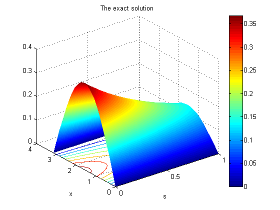
(a)

(b)

Figure 1: The exact solution $u_{ex}\left(x,t,s\right)=e^{-2t-s}\sin x$ shown in (a) in comparison with the approximate solution (30)-(31) shown in (b) at $t=\dfrac{1}{2}$ for Example 1.

(a)

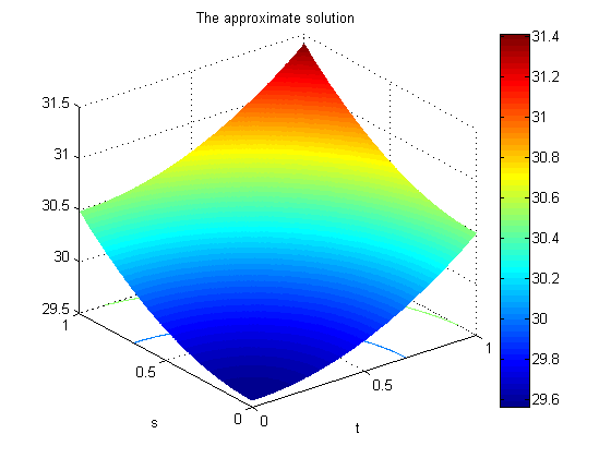
(b)

Figure 2: The exact solution $u_{ex}\left(x,t,s\right)=\left(t^{2}+s^{2}+32\right)\cos\left(\dfrac{x}{2}\right)$ shown in (a) in comparison with the approximate solution (32)-(33) shown in (b) at $x=\dfrac{\pi}{4}$ for Example 2.

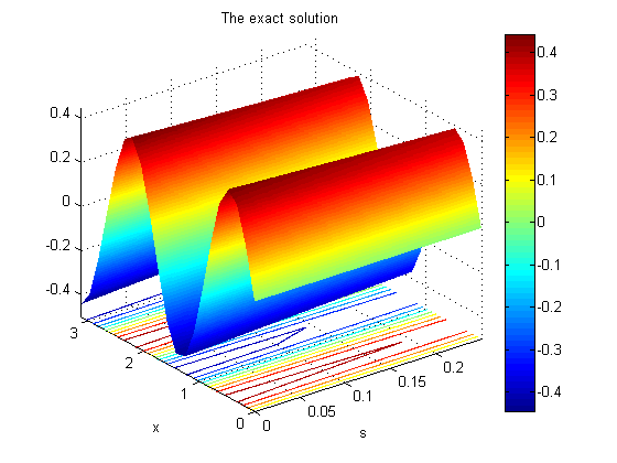
(a)

(b)

Figure 3: The exact solution $u_{ex}\left(x,t,s\right)=\dfrac{1}{4}\left(e^{-t}+e^{-s}\right)\sin\left(\dfrac{7x}{2}\right)$ shown in (a) in comparison with the approximate solution (34)-(36) shown in (b) at $t=\dfrac{1}{4}$ for Example 3.

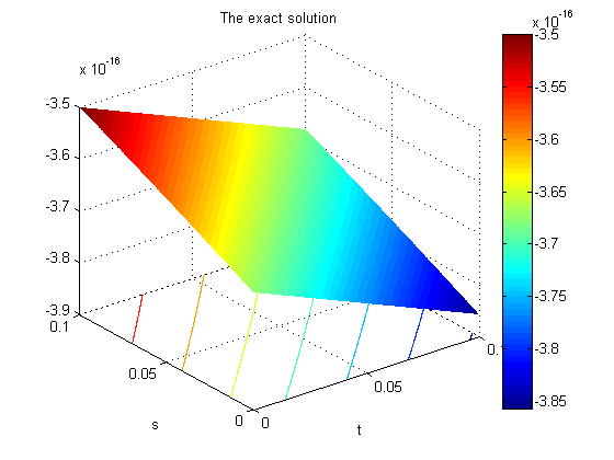
(a)

(b)

Figure 4: The exact solution $u_{ex}\left(x,t,s\right)=\left(\sin t+1+e^{-s}\right)\cos\left(3x\right)$ shown in (a) in comparison with the approximate solution (38)-(39) shown in (b) at $x=\dfrac{\pi}{2}$ for Example 4.

Denoting $E=u_{ex}-u$, we compute the discrete $l_{2}$-norm and $l_{\infty}$-norm of $E$ by

$$\left\|E\right\|_{l_{2}}=\sqrt{\frac{1}{\mathcal{\left|G\right|}}\sum_{\chi_{G}\in\mathcal{G}}\left|E\left(\chi_{G}\right)\right|^{2}},\quad\left\|E\right\|_{l_{\infty}}=\max_{\chi_{G}\in\mathcal{G}}\left|E\left(\chi_{G}\right)\right|,$$ (40)

where $\mathcal{G}=\left\{\chi_{G}\right\}$ is a set of $\left(L+1\right)M^{2}$ points on uniform grid $\left[0,\pi\right]\times\left(0,T\right]\times\left(0,T\right]$ and $\left|\mathcal{G}\right|$ cardinality of $\mathcal{G}$.

In our computations, we always fix $j_{0}=5$ and $L=20$. The comparison between the exact solutions and the approximate solutions for the examples respectively are shown in Figure 1-Figure 4 in graphical representations. As in these figures, we can see that the exact solution and the approximate solution are close together. Furthermore, convergence is observed from the computed errors in Table 1-Table 4 for Example 1-Example 4, respectively, which is reasonable for our theoretical results.

Table 1: Numerical results (40) for Example 1 with $L=20$.

	$M=50$	$M=100$	$M=200$	$M=400$
$\left\|E\right\|_{l_{2}}$	1.51608045E-03	7.55346287E-04	3.85041789E-04	1.88342949E-04
$\left\|E\right\|_{l_{\infty}}$	3.84188903E-03	1.92287169E-03	9.61845810E-04	4.81024266E-04

Table 2: Numerical results (40) for Example 2 with $L=20$.

	$M=50$	$M=100$	$M=200$	$M=400$
$\left\|E\right\|_{l_{2}}$	6.53270883E-03	3.26622222E-03	1.63312276E-03	8.16570001E-04
$\left\|E\right\|_{l_{\infty}}$	2.26666504E-02	1.13406619E-02	5.67215954E-03	2.83653620E-03

Table 3: Numerical results (40) for Example 3 with $j_{0}=5,L=20$.

	$q=2,M=50$	$q=3,M=100$	$q=4,M=200$	$q=5,M=400$
$\left\|E\right\|_{l_{2}}$	5.82730398E-03	2.90030629E-03	1.44171369E-03	7.18708022E-04
$\left\|E\right\|_{l_{\infty}}$	1.16425665E-02	5.85110603E-03	2.91848574E-03	1.45728672E-03

Table 4: Numerical results (40) for Example 4 with $j_{0}=5,L=20$.

	$q=2,M=50$	$q=3,M=100$	$q=4,M=200$	$q=5,M=400$
$\left\|E\right\|_{l_{2}}$	5.45295363E-03	2.69804976E-03	1.34196386E-03	6.69222399E-04
$\left\|E\right\|_{l_{\infty}}$	1.48732036E-02	7.42289652E-03	3.70802189E-03	1.85315435E-03

5 Conclusion

In this paper, we have studied the numerical method for solving a class of nonlinear ultraparabolic equations in abstract Hilbert spaces, namely problem (1)-(2). Our numerical approach is based on finite difference method and representation by Fourier series. The method not only serves the ultraparabolic problems in multi-space dimension but also deals with a wide class of nonlinear ultraparabolic problems that many recent studies do not cover. Moreover, it is useful in numerical simulations when one wants to construct a stable, reliable and fast convergent approximation. Some stability results and error estimates are obtained. Lots of numerical examples are showed to see the efficiency of the method.

In fact, it should be stated that Fourier series expression of solution may lead a limitation of the method for applications in a complicated domain where a solution cannot be expressed by a certain series. On the other hand, numerical method for a class of nonlinear equations in a large time scale with a better convergence rate should be developed. All of these issues will be surveyed in a further research.

Competing interests

The authors declare that they have no competing interests.

Author’s contributions

All authors, VAK, LTL, NTYN and NHT contributed to each part of this work equally and read and approved the final version of the manuscript.

References

- [1] F. Ternat, O. Orellana, P. Daripa, Two stable methods with numerical experiments for solving the backward heat equation, Applied Numerical Mathematics 61 (2011) 266-284.
- [2] N. H. Tuan, Stability estimates for a class of semi-linear ill-posed problems, Nonlinear Analysis: Real World Applications 14 (2013) 1203-1215.
- [3] G. Akrivis, M. Crouzeix, and V. Thomée, Numerical methods for ultraparabolic equations, Calcolo, vol. 31, no. 3-4, pp. 179–190, 1994.
- [4] Fadugba S. E., Edogbanya O. H., Zelibe S. C., Crank Nicolson Method for Solving Parabolic Partial Differential Equations, International Journal of Applied Mathematics and Modeling, Vol.1, No. 3, 8-23, 2013.
- [5] F. Zouyed, F. Rebbani, A modified quasi-boundary value method for an ultraparabolic ill-posed problem, J. Inverse Ill-Posed Probl., Volume 0, 1569-3945, 2014.
- [6] A. Ashyralyev and S. Yilmaz, An Approximation of Ultra-Parabolic Equations, Abstract and Applied Analysis, vol. 2012, Article ID 840621, 14 pages, 2012.
- [7] D. D. Trong, N. T. Long, A. P. N. Dinh, Nonhomogeneous heat equation: Identification and regularization for the inhomogeneous term, J. Math. Anal. Appl. 312 (2005) 93–104.
- [8] Q. Deng , T. G. Hallam , An age structured population model in a spatially heterogeneous environment: Existence and uniqueness theory, Nonlinear Anal. 2006; 65, 379-394.
- [9] M. D. Francesco, A. Pascucci, A continuous dependence result for ultraparabolic equations in option pricing, J. Math. Anal. Appl. 336 (2007) 1026–1041.
- [10] A. I. Kozhanov, On the Solvability of Boundary Value Problems for Quasilinear Ultraparabolic Equations in Some Mathematical Models of the Dynamics of Biological Systems, Journal of Applied and Industrial Mathematics, 2010, Vol. 4, No. 4, pp. 512–525.
- [11] S. A. Tersenov, Well-posedness of boundary value problems for a certain ultraparabolic equation, Siberian Mathematical Journal, Vol. 40, No. 6, 1999.
- [12] Alkis S. Tersenov, Ultraparabolic equations and unsteady heat transfer, J.evol.equ. 5 (2005) 277–289.
- [13] W. H. Press et al., Numerical recipes in Fortran 90, 2nd ed., Cambridge University Press, New York, 1996.
- [14] V. S. Dron’ and S. D. Ivasyshen, Properties of the fundamental solutions and uniqueness theorems for the solutions of the Cauchy problem for one class of ultraparabolic equations, Ukrainian Mathematical Journal, Vol. 50, No. 11. 1998.
- [15] M. A. Ragusa, On weak solutions of ultraparabolic equations, Nonlinear Analysis 47 (2001) 503–511.
- [16] L. Lorenzi, An Identification Problem for an Ultraparabolic Integrodifferential Equation, Journal of Mathematical Analysis and Applications 234, 417–456 (1999).
- [17] M. Bramanti and M. C. Cerutti, Estimates for Some Ultraparabolic Operators with Discontinuous Coefficients, Journal of Mathematical Analysis and Applications 200, 332–354 (1996).
- [18] Michael D. Marcozzi, Extrapolation discontinuous Galerkin method for ultraparabolic equations, Journal of Computational and Applied Mathematics 224 (2009) 679–687.
- [19] Tarik Mohamed Touaoula and Noureddine Ghouali, Gradient Estimates for Solutions of Ultraparabolic Equations, Mediterr. j. math. 5 (2008), 101–111.
- [20] G. E. Uhlenbeck, L. S. Ornstein, On the theory of the Brownian motion, Phys. Rev. 36 (1930) 823-841.
- [21] R. E. Showalter, Hilbert Space Methods for Partial Differential Equations, Electronic Journal of Differential Equations, Monograph 01, 1994.
- [22] M. Ghergu, V. D. Radulescu, Nonlinear PDEs: Mathematical Models in Biology, Chemistry and Population Genetics, Springer Monographs in Mathematics, 2011.
- [23] A. Ashyralyev, S. Yilmaz, Modified Crank–Nicholson difference schemes for ultra-parabolic equations, Computers and Mathematics with Applications 64 (2012) 2756–2764.