Orbital magnetic moments in insulating Dirac systems: Impact on magneto-transport in graphene van der Waals heterostructures

Abstract

In honeycomb Dirac systems with broken inversion symmetry, orbital magnetic moments coupled to the valley degree of freedom arise due to the topology of the band structure, leading to valley-selective optical dichroism. On the other hand, in Dirac systems with prominent spin-orbit coupling, similar orbital magnetic moments emerge as well. These moments are coupled to spin, but otherwise have the same functional form as the moments stemming from spatial inversion breaking. After reviewing the basic properties of these moments, which are relevant for a whole set of newly discovered materials, such as silicene and germanene, we study the particular impact that these moments have on graphene nano-engineered barriers with artificially enhanced spin-orbit coupling. We examine transmission properties of such barriers in the presence of a magnetic field. The orbital moments are found to manifest in transport characteristics through spin-dependent transmission and conductance, making them directly accessible in experiments. Moreover, the Zeeman-type effects appear without explicitly incorporating the Zeeman term in the models, i.e., by using minimal coupling and Peierls substitution in continuum and the tight-binding methods, respectively. We find that a quasi-classical view is able to explain all the observed phenomena.

I Introduction

One of the more intriguing recent developments in the field of graphene research is the artificial generation of properties that are otherwise vanishing in intrinsic samples. For instance, carrier mass can be created by sandwiching graphene with hexagonal boron nitride (hBN), in which case a gap arises for sufficiently aligned layers.hunt13 ; woods14 The occurrence of the gap is dictated by the interplay of the elastic energy of the graphene lattice, and the potential energy landscape stemming from hBN.jung14 The energetically preferred commensurate structure, in which a carbon atom sits on top of a boron atom, will maximize its area at the expense of other stacking configurations by stretching the graphene layer. This in turn leads to the appearance of an average gap in the resulting van der Waals heterostructure.woods14

On the other hand, it was postulated that spin-orbit coupling (SOC) in graphene can be enhanced by hydrogen adsorption, which forces local rehybridization of bonds.neto2009 Note that quantum spin Hall transport signatures introduced by random adatoms are well described by models taking into account a renormalized and uniform SOC.shevtsov12 ; jiang12 Moreover, the proximity effect caused by an appropriate substrate was speculated to lead to SOC enhancement as well. Both of these mechanisms were recently confirmed experimentally, opening new avenues for theoretical research.ozy13 ; avsar14

While in graphene the carrier mass and SOC have to be artificially engineered, they are ubiquitous in other group IV monolayers such as silicene, germanene, and stanene, thanks to their buckled structure and the heavier constituent atoms.cahangirov09 ; liu11 ; xu13 Given their honeycomb lattice, they also belong to the same class of materials as graphene, with relativistic quasiparticles described by the Dirac equation. From the theoretical point of view, both of the aforementioned parameters appear in a similar form in the low-energy continuum picture. They are captured by staggered potential terms $\Delta$ and $\Delta_{SO}$ in the case of mass and SOC, respectively.footnote The term ”staggered potential” originates in the language of the tight-binding method, and it refers to the breaking of the sublattice symmetry by a traceless potential. Unlike SOC, for which the staggered potential changes sign depending on the spin and valley of the electron, $\Delta$ opens up a topologically trivial band gap in the vicinity of the $K$ and $K^{\prime}$ points through inversion symmetry breaking.kane05a

At the same time, however, the inversion symmetry breaking leads to a nontrivial alteration of the semiclassical equations of motion on a honeycomb lattice.chang95 ; xiao07 The quantum corrections, which reflect the impact of the Berry phase, and are therefore topological in nature, are twofold. On the one hand, when subjected to an electric field in the plane, massive Dirac fermions will attain a velocity component transverse to the field, which is opposite in the two valleys, thus giving rise to the valley Hall effect. This effect was recently observed experimentally in a ${\rm MoS}_{2}$ device, as well as in graphene-hBN heterostructures.mak14 ; gorbachev14 On the other hand, self-rotation of electron wavepackets near the two valleys will produce valley-contrasting orbital magnetism.xiao07

It is well established that the valley Hall and intrinsic spin Hall effects share the same origin, reflecting the Berry curvature properties of the underlying insulating systems, generated by $\Delta$ and $\Delta_{SO}$ terms, respectively. Therefore, the two Hall effects are fully analogous.feng12 ; xiao12 Valley-contrasting magnetism was first reported in Ref. xiao07, . On the other hand, we recently found evidence of the corresponding spin-contrasting magnetism in transport calculations involving spin-orbit barriers in bulk graphene,grujic14 which motivated us to explore the subject more thoroughly. These orbital magnetic moments were previously investigated in a more generalized analysis on the abundance of Hall effects (and the accompanying wealth of orbital magnetization), found in multilayer graphene systems in Ref. zhang11, . There, the electron-electron interaction leads to various broken symmetry phases, denoted by the general term ”pseudospin ferromagnetism”,min08 ; zhang10 ; nand10 ; jung11 which are captured with a diverse set of mass terms in the low-energy continuum approximation, in models analogous to the ones studied in this paper.

This emerging orbital magnetism is a mechanism that effectively alters the Zeeman energy, and it is the subject of this paper, particularly the moments associated with spin-orbit coupling in monolayer Dirac systems. We first review how the intrinsic SOC in honeycomb monolayers gives rise to orbital magnetic moments coupled to spin, in the same way in which inversion symmetry breaking gives rise to moments coupled to the valley degree of freedom. These moments are completely analogous in nature, and they share exactly the same functional form, apart from coupling to different degrees of freedom. We derive expressions for the moments using both tight-binding and continuum theories, and we show their impact on the Landau level (LL) quantization in the presence of a magnetic field.

Finally, we investigate the influence of the moments on the magneto-transport properties, where we look at the transmission through a barrier with enhanced spin-orbit coupling in graphene. Such a barrier could be realized by an appropriately formed van der Waals heterostructure in an otherwise fully ultrarelativistic material.shevtsov12 ; jiang12 ; ozy13 ; avsar14 We discuss this case in great detail from the semiclassical point of view, and we present conclusions that are of practical relevance, namely how the device conductance is affected by orbital magnetism. In the end, we show that the results are identical whether one uses the continuum Dirac theory or the tight-binding nonequilibrium Green function method (TB NEGF) when calculating the transport properties. Remarkably, both approaches yield Zeeman-type transport signatures while employing the magnetic field only through kinetic terms, without actually enforcing the coupling of the spin with the magnetic field, which reflects the orbital nature of the magnetic moments.

II Orbital moments in the tight binding picture

We start with the low-energy tight binding Kane-Mele Hamiltonian valid for a whole set of Dirac materials with prominent intrinsic spin-orbit coupling,kane05

$$H=\hbar v_{F}\left[\tau k_{x}\sigma_{x}+k_{y}\sigma_{y}\right]+s\tau\Delta_{SO}\sigma_{z},$$ (1)

where $v_{F}$ is the Fermi velocity, $\Delta_{SO}$ is spin-orbit coupling, $\sigma_{z}$ is a Pauli matrix operating in the sublattice subspace, $s=+1/-1$ labels the spin $\uparrow/\downarrow$, and $\tau=+1/-1$ labels the valley $K/K^{\prime}$. As already mentioned this form of SOC is universal to all group IV monolayers other than graphene, in which on the other hand it could be artificially generated. Note that here $k_{x}$ and $k_{y}$ are only parameters, and not operators. The dispersion relations extracted from Eq. (1) are shown by solid black curves in Fig. 1(a).

The Hamiltonian (1) describes a two-state, electron-hole symmetric system. For such systems, the orbital magnetic moment ($m$) is directly proportional to the Berry curvature ($\Omega$), $m\sim\Omega$.xiao07 ; zhang11 ; yao08 On the other hand, the system is also time-reversal invariant, and since we disregard the staggered potential $\Delta$ at the moment, inversion symmetry is not broken either. Since for spatial-inversion and time-reversal symmetric systems Berry curvature vanishes,xiao10 ; chang08 one might conclude that the orbital moments must vanish as well. However, it is rarely stressed that this only holds for spinless electrons, which is not the case considered here.gradhand12 In fact, the Hamiltonian (1) describes a topological insulator, having a non-zero and opposite Chern number for opposite spins.kane05 This is because the Kane-Mele model is formed by two opposite copies of the Haldane model,haldane88 thus breaking the time-reversal symmetry separately in each spin sector. Since the Chern number is obtained as an integral of $\Omega$ over the Brillouin zone, the Berry curvature is nontrivial, and consequently, the orbital magnetic moments will be nonzero.

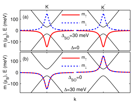
Figure 1: The orbital magnetic moments of the spin-up (spin-down) states shown by thick red (dashed blue) lines, and the corresponding low-energy band structure, shown in black, for: (a) $\Delta=0$ and $\Delta_{SO}=30$ meV, and (b) $\Delta=30$ meV and $\Delta_{SO}=0$. Note that in (b) the orbital magnetic moments for the two spins are equal, due to the absence of SOC.

The orbital moments are perpendicular to the monolayer, and originate from the self-rotation of the electron wave packet around its center of mass, and they can be obtained from the tight binding Bloch eigenfunctions $|u\left(\mathbf{k}\right)\rangle$xiao07 ; xiao10 ; zhang11

$$m=-i\frac{e}{2\hbar}\langle\mathbf{\nabla}_{\mathbf{k}}u|\times\left[H-E\left(\mathbf{k}\right)\right]|\mathbf{\nabla}_{\mathbf{k}}u\rangle,$$ (2)

which makes their topological origin much clearer. For the particular Hamiltonian in Eq. (1), we have

$$|u\left(\mathbf{k}\right)\rangle=\left(\begin{array}[]{c}\sqrt{\frac{E+s\tau\Delta_{SO}}{2E}}\\ \tau\sqrt{\frac{E-s\tau\Delta_{SO}}{2E}}e^{i\tau\phi}\end{array}\right),$$ (3)

where $E$ is the electron energy, and $\phi=\arctan k_{y}/k_{x}$. It is then straightforward to show that the expression for the magnetic moments that arise from the spin-orbit coupling reads

$$m=-s\frac{e\hbar v_{F}^{2}\Delta_{SO}}{2\left(\Delta_{SO}^{2}+\hbar^{2}v_{F}^{2}k^{2}\right)}.$$ (4)

Variations of the orbital moments in the vicinity of the Dirac points are shown for both spins in Fig. 1(a). They are maximum near the band edges, decay away from the two Dirac points, and are obviously opposite for opposite spins.

One can compare these moments with the valley-contrasting moments, arising for $\Delta_{SO}=0$ and $\Delta\neq 0$.xiao07 ; xiao10 Their magnitude is given by

$$m=-\tau\frac{e\hbar v_{F}^{2}\Delta}{2\left(\Delta^{2}+\hbar^{2}v_{F}^{2}k^{2}\right)},$$ (5)

and they are depicted in Fig. 1(b). It is clear that the two sets of moments share a similar functional form, except the former couple to spin, while the latter couple to the valley degree of freedom.zhang11 The energy region where the moments are prominent was termed the Berry curvature hot spot in Ref. gorbachev14 There it was unequivocally shown that the gap in well-aligned graphene-hBN van der Waals heterostructures is accompanied by the introduction of nontrivial Berry curvature.

Finally, in the case of both nonzero $\Delta_{SO}$ and $\Delta$, and in the low energy limit, the magnetic moment is given by

$$m=-\frac{e\hbar v_{F}^{2}}{2\left(s\Delta_{SO}+\tau\Delta\right)}.$$ (6)

The orbital magnetic moments are responsible for the optical selection rules of light absorption in Dirac materials, through the so-called circular dichroism effect.yao08 ; xiao12 ; ezawa12 Note that the orbital moments in Eq. (4) can dominate the Zeeman response of a system, since they can be orders of magnitude stronger than the free-electron Bohr magneton for realistic SOC strengths found in typical Dirac materials.xiao07 ; xiao10 ; zhang11 ; jung11 In other words, they will lead to a renormalization of the Landé $g$ factor, which was recently observed for transition metal dichalcogenides from first-principles calculations.kormanyos14

III Landau levels, pseudospin polarization and orbital moments in the continuum picture

III.1 Landau levels

We proceed with the case of an applied perpendicular magnetic field ${\bf B}=B{\bf e}_{z}$ in bulk graphene, which is included in the Hamiltonian through minimal coupling

$$H=\hbar v_{F}\left[\tau k_{x}\sigma_{x}+(k_{y}+\frac{e}{\hbar}A_{y})\sigma_{y}\right]+s\tau\Delta_{SO}\sigma_{z}+\Delta\sigma_{z}.$$ (7)

This equation could be employed to solve the electron spectrum in the Dirac system in the presence of $\Delta_{SO}$, $\Delta$, and magnetic field. It will subsequently lead us to resolve the magnetic moments. Here, the Landau gauge $\mathbf{A}=\left(0,A_{y}\right)$ with $A_{y}=Bx$ is chosen. In this gauge, $k_{y}$ is a good quantum number and the solutions have the form $\Psi(x,y)=\exp(ik_{y}y)\left(\psi_{A}(x),\psi_{B}(x)\right)^{T}$. Introducing $\hbar v_{F}\epsilon=E$, $\hbar v_{F}\delta=s\tau\Delta_{SO}+\Delta$, one can obtain the LLs in the infinite graphene sheet. In solving the LL spectrum it is useful to adopt the operators $b_{\tau}^{\dagger}=-i(l_{B}/\sqrt{2})\left(\tau k_{x}+ik_{y}+ieA_{y}/\hbar\right)$ and $b_{\tau}$, where $l_{B}=\sqrt{\hbar/eB}$ denotes the magnetic length. $b_{\tau}^{\dagger}$ and $b_{\tau}$ are the bosonic ladder operators, and they satisfy $\left[b_{\tau},b_{\tau}^{\dagger}\right]=\tau$. It could be useful to define these operators such that they fully correspond to the standard ladder operators of the quantum harmonic oscillator (QHO) shifted by $x_{0}=k_{y}l_{B}^{2}$ and having the mass $m=\hbar^{2}/l_{B}^{4}k$. Then the eigenstates will be given by the standard (obviously shifted and rescaled) QHO solutions

$$\langle x|n\rangle=\frac{1}{\sqrt{2^{n}n!}}e^{-\left(x/l_{B}+k_{y}l_{B}\right)^{2}/2}H_{n}\left(\frac{x}{l_{B}}+k_{y}l_{B}\right),$$ (8)

where $H_{n}$ are Hermite polynomials. The problem can now be solved in terms of these solutions for the case of the regular two-dimensional (2D) electron gas in a magnetic field, having in mind that $b_{1}^{\dagger}|n\rangle=\sqrt{n+1}|n+1\rangle$, $b_{1}|n\rangle=\sqrt{n}|n-1\rangle$ and $b_{1}|0\rangle=0$, and that the ladder operators change character in the $K^{\prime}$ valley. The system of coupled equations with ladder operators is now given by

$$\delta\psi_{A}-i\frac{\omega_{c}}{v_{F}}b_{\tau}\psi_{B} =\epsilon\psi_{A},$$ (9)

$$i\frac{\omega_{c}}{v_{F}}b_{\tau}^{\dagger}\psi_{A}-\delta\psi_{B} =\epsilon\psi_{B},$$ (10)

where $\omega_{c}=\sqrt{2}v_{F}/l_{B}$ is the cyclotron frequency for Dirac-Weyl electrons. Then for $n\geq 1$ the energies of the LLs are given by

$$\epsilon_{n,s,\tau,\pm}=\pm\sqrt{\delta^{2}+n\omega_{c}^{2}/v_{F}^{2}}.$$ (11)

The $s$ and $\tau$ quantum numbers are contained implicitly in the definition of $\delta$. The joint spinor for the two valleys can be written as

$$|n,s,\tau,\pm\rangle=\left(\begin{array}[]{c}|n-\frac{\tau}{2}-\frac{1}{2}\rangle\\ \pm i\left[\frac{\omega_{c}\sqrt{n}}{\left(\epsilon+\tau\delta\right)v_{F}}\right]^{\tau}|n+\frac{\tau}{2}-\frac{1}{2}\rangle\end{array}\right).$$ (12)

The case of $n=0$ needs special attention, since the solution, Eq. (12), is not valid in this case. Then, the appropriate choice for the solution is

$$|0,s,\tau\rangle=\left(-\tau/2+1/2,\tau/2+1/2\right)^{T}|0\rangle,$$ (13)

while the energies are expressed as tabert13

$$\epsilon_{0,s,\tau}=-\tau\delta.$$ (14)

It is worth pointing out however, that observation of the conductance plateaus corresponding to the derived spectrum can depend on the symmetry class of the disorder present in the samples.ostrovsky08 Note also that these eigenvectors and eigenvalues reduce to the ones for the massless fermions, under the requirement $\delta\rightarrow 0$, collapsing the level (14) to zero energy. Nevertheless, massless fermions can also display quantum Hall signatures, such as a magnetic-field-independent plateau at zero filling factor, which originate from valley mixing scattering processes.ostrovsky08

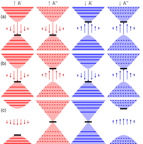
Figure 2: Several lowest Landau levels of all spin and valley flavors for (a) $\Delta_{SO}=30$ meV and $\Delta=0$, (b) $\Delta_{SO}=0$ and $\Delta=30$ meV, and (c) $\Delta_{SO}=\Delta=30$ meV. The $n=0$ Landau level is depicted by the horizontal solid black line. Also shown are the bulk bands as red (spin up) and blue (spin down) shaded regions, as well as the sketch of the corresponding orbital moments, with the length of the arrow being proportional to the intensity.

Thus the SOC and mass terms split and shift the zeroth LLs away from zero energy as depicted in Fig. 2, which shows the low-lying Landau levels for (a) only $\Delta_{SO}\neq 0$, (b) only $\Delta\neq 0$ and (c) $\Delta_{SO}=\Delta\neq 0$ at $B=2$ T. We also depict the bands, as well as the emerging magnetic moments, given by Eqs. (4) and (5). The orientation of the moments is related to the position of the $n=0$ Landau level, which is shown by the horizontal solid black lines. Note that the zeroth LLs always reside on the edges of the appropriate bands. The duality $\Delta_{SO}\leftrightarrow\Delta$, $s\leftrightarrow\tau$ present in Eq. (14) is evident in Fig. 2. In other words, SOC couples the LLs to spin in the same way that mass couples them to the valley degree of freedom.tabert13 ; krsta12 ; lado13 The state depicted in Fig. 2(c) is dubbed spin-valley-polarized metal,ezawa12a and it hosts both a massless (lacking the orbital moments) and a massive relativistic Landau spectrum. It can appear in silicene subjected to a perpendicular electric field, for instance. On the other hand, in transition-metal dichalcogenides, both parameters are inherently present, with $\Delta>\Delta_{SO}$, and SOC splits only the LLs in the valence band, yielding a unique set of Hall plateaus.li13

III.2 Orbital moments

The underlying explanation for the behavior of the LL spectrum can be sought in the existence of orbital magnetic moments.xiao07 ; cai13 ; koshino10 In a similar fashion to Ref. koshino10, , we can obtain the effective Bohr’s magneton in the presence of $\Delta_{SO}$, starting from the Dirac-Weyl equation, and expanding near the conduction band bottom. We first point out that near the bottom of the conduction bands, the sublattice pseudospins get polarized perpendicular to the graphene sheet, with the majority of the weight concentrated on the A (B) sublattice for $\delta>0$ ($\delta<0$). Likewise, at the top of the valence band, most of the weight is found on the A (B) sublattice for $\delta<0$ ($\delta>0$). This is obvious for the zeroth LLs, and it occurs in the $\delta=0$ limit as well,goerbig11 ; grujic11 but to see it for higher levels it is helpful to derive the expectation value for the sublattice pseudospin,

$$\langle n,s,\tau,\pm|\sigma_{z}|n,s,\tau,\pm\rangle=\frac{\delta}{\epsilon}.$$ (15)

which is exactly the same as in the absence of SOC and magnetic field,leyla11 only now it is to be used for the discrete energy values corresponding to the Landau levels. Therefore, perfect pseudospin polarization is achieved in the bottom (top) of the conduction (valence) band.

On the other hand, decoupling the Dirac equation gives

$$\left[k_{x}^{2}+\left(k_{y}+\frac{x}{l_{B}^{2}}\right)^{2}\pm\frac{\tau}{l_{B}^{2}}\right]\psi_{A/B}=\left(\epsilon^{2}-\delta^{2}\right)\psi_{A/B}.$$ (16)

Therefore, there is a spatially uniform term proportional to the magnetic field, with opposite signs on opposite sublattices and opposite valleys. Consider the importance of this term for states whose sublattice pseudospin mostly lies in the graphene plane, i.e. for states far away from the band gap, Eq. (15). For such states, the two signs play a tug of war, effectively canceling each other out. However, near the band gap, sublattice polarization occurs, and the term corresponding to a majority sublattice starts dominating over the other, giving rise to an effective paramagnetic moment. For instance, when $\delta>0$ sublattice A dominates for low electron energies, and the upper sign starts impacting the electron motion. To fully appreciate this fact, and to write the equation in a manifestly paramagnetic form, one needs to perform a low energy expansion for the equation of the majority sublattice. After reintroducing $E$, $\Delta$, and $\Delta_{SO}$ explicitly, we can write $E=\xi+\left(s\tau\Delta_{SO}+\Delta\right)$ for $\delta>0$, and $E=\xi-\left(s\tau\Delta_{SO}+\Delta\right)$ for $\delta<0$. Taking the limit $\xi\rightarrow 0$, the following equation is obtained for the bottom of the conduction band

$$\left[\frac{p_{x}^{2}}{2m_{eff}}+\frac{\left(p_{y}+eA_{y}\right)^{2}}{2m_{eff}}+\frac{e\hbar v_{F}^{2}B}{2\left(s\Delta_{SO}+\tau\Delta\right)}\right]\psi=\xi\psi.$$ (17)

where $m_{eff}=\left|s\tau\Delta_{SO}+\Delta\right|/v_{F}^{2}$ is the electron effective mass due to the band gap. This is the form of the Schrödinger equation in the presence of a magnetic field in which the emerging magnetic moments are obviously manifested. Once again, we see the duality of the orbital moments of the same nature as mentioned previously in the case of LLs: the moments are coupled to SOC through spin and to mass through the valley degree of freedom. Moreover, it is obvious that the expression for the magnetic moment is equal to the results of the low energy expansion given in Eq. (6). Having in mind that these moments effectively shift the low energy parabolic bands, one can use the same argument as in Ref. cai13, to show that the separation between the lowest LL and the bottom of each shifted band is for each spin, valley and band to first order equal to half the separation between this and the first excited LL. This is in analogy with the LLs in a 2D massive-electron gas, where the lowest level sits at half the cyclotron frequency.cai13 ; koshino10 The difference for higher energy LLs is a consequence of the deviation of the dispersion from the quadratic one.

IV Manifestation of orbital moments on magneto-transport

We proceed with considering how the emerging magnetic moments affect the transport properties. In particular, we analyze transport through a single 1D barrier in bulk graphene, extending from $x=0$ up to $x=W$, and along the $y$ direction, in which the intrinsic SOC is modified. The magnetic field is included only in the barrier, so we choose the following vector potential (within the Landau gauge)

$$A_{y}=\begin{cases}0&x<0\\ Bx&0\leq x\leq W\\ BW&x>W\end{cases}.$$ (18)

The explicit derivation of the transmission coefficient is given in Appendix A.

Since we analyze a barrier made exclusively out of SOC, the valley degree of freedom plays no role in the electron transmission, which can be concluded from the theory presented in Secs. II and III. Therefore, the contour plots of the transmission coefficient $T=\left|t\right|^{2}$, for the two spin flavors, and for the $200$-nm wide barrier as a function of energy and the incident angle of the incoming electron, are shown in Fig. 2. Each horizontal panel in this figure corresponds to a specific value of the magnetic field, which is $0$, $0.1$, $0.2$ to $0.3$ T from top to bottom. Because of the duality $\Delta_{SO}\leftrightarrow\Delta$ and $s\leftrightarrow\tau$, the results presented below also apply for transmission through a barrier when $\Delta\neq 0$ and $\Delta_{SO}=0$. But for this case the spin and valley quantum numbers should be interchanged.

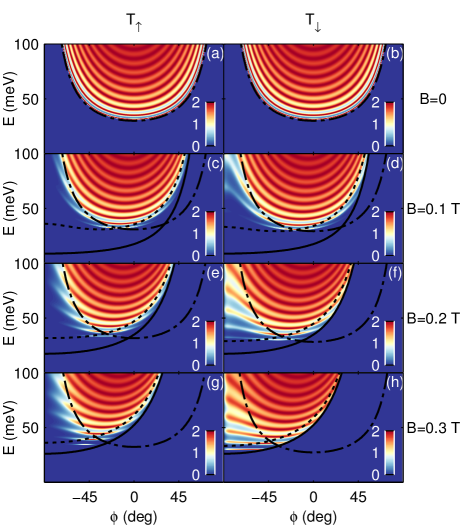
Figure 3: Contour plots of the transmission coefficient as function of incident angle and energy for $\Delta_{SO}=30$ meV, $\Delta=0$ and $W=200$ nm. The magnetic field equals $0$ T in (a-b), $0.1$ T in (c-d), $0.2$ T in (e-f), and $0.3$ T in (g-h). The results are shown for both spin orientations. The semiclassical critical boundaries $\epsilon_{cr0}$ and $\epsilon_{crW}$ are depicted by dash-dotted and dotted lines, respectively.

For both barrier types, we found that the magnetic field causes cyclotron motion, whose main feature is the appearance of a transmission window dependent on energy and incident angle $\phi$.masir08 ; grujic14 Outside of this window, the waves after the barrier become evanescent, and therefore no transmission takes place. This occurs when the longitudinal momentum $k_{x}^{\prime}=\sqrt{\epsilon^{2}-k_{y}^{\prime}}$ of each electron state in the region after the barrier becomes imaginary. The transmission window is given by

$$\epsilon>\frac{\gamma}{1-\sin\phi},$$ (19)

where $\gamma=W/l_{B}^{2}$. The transmission windows for different $B$ are shown by solid black curves in Fig. 3.

When the magnetic field increases, the transmission asymmetry with respect to the incident angle becomes larger, due to the cyclotron motion, as shown in Fig. 3. Besides, whereas transmission coefficients are identical for both spins when no magnetic field is present, $T_{\uparrow}$ and $T_{\downarrow}$ differ when $B\neq 0$, which is a consequence of the SOC-induced magnetic moments. In fact, it is clear from Eq. (16) that a quasi-classical longitudinal momentum $q_{x}$

$$q_{x}\left(x\right)=\sqrt{\epsilon^{2}-\delta^{2}-\left(k_{y}+x/l_{B}^{2}\right)^{2}-s/l_{B}^{2}}$$ (20)

can be assigned to the sublattice-polarized states.

In order to understand the effects of the emerging magnetic moments on the transmission characteristics, it is instructive to investigate how classical turning points vary with $\epsilon$ and $\phi$. Those turning points are extracted from $q_{x}\left(x\right)=0$, where $q_{x}$ is given by Eq. (20), and are given by

$$x_{1,2}=-\epsilon l_{B}^{2}\sin\phi\mp l_{B}^{2}\sqrt{\epsilon^{2}-\delta^{2}-\mu},$$ (21)

where $\mu=s/l_{B}^{2}$ is the magnetic moment term which appears in the expression for the quasi-classical momentum in Eq. (20). Given that the barrier extends from $0$ to $W$, the condition that no turning points are found within the barrier is obtained by requiring $x_{1}<0$ and $x_{2}>W$. The former condition leads to

$$x_{1}<0\Rightarrow\begin{cases}\epsilon>\frac{\sqrt{\delta^{2}+\mu}}{\cos\phi},\quad\phi<0\\ \epsilon>\sqrt{\delta^{2}+\mu},\quad\phi>0\end{cases},$$ (22)

while the latter results in

$$x_{2}>W\Rightarrow\begin{cases}\epsilon>\sqrt{\delta^{2}+\mu},\quad\epsilon\sin\phi+\gamma<0\\ \epsilon>\frac{\gamma\sin\phi+\sqrt{\gamma^{2}+\left(\delta^{2}+\mu\right)\cos^{2}\phi}}{\cos^{2}\phi},\quad\epsilon\sin\phi+\gamma>0\end{cases}.$$ (23)

On the other hand, both classically forbidden and classically allowed regions will be present in the barrier if $0<x_{1}<x_{2}<W$. The two extreme cases of vanishing allowed regions occur when the leftmost turning point approaches the right interface of the barrier

$$x_{1}<W\Rightarrow\begin{cases}\epsilon>\frac{\gamma\sin\phi+\sqrt{\gamma^{2}+\left(\delta^{2}+\mu\right)\cos^{2}\phi}}{\cos^{2}\phi},\quad\epsilon\sin\phi+\gamma<0\\ \epsilon>\sqrt{\delta^{2}+\mu},\quad\epsilon\sin\phi+\gamma>0\end{cases},$$ (24)

and when the rightmost turning point approaches the left barrier interface

$$x_{2}>0\Rightarrow\begin{cases}\epsilon>\sqrt{\delta^{2}+\mu},\quad\phi<0\\ \epsilon>\frac{\sqrt{\delta^{2}+\mu}}{\cos\phi},\quad\phi>0\end{cases}.$$ (25)

From the angle dependent functions in the last four equations one might define the critical energies

$$\epsilon_{cr0}=\frac{\sqrt{\delta^{2}+\mu}}{\cos\phi},$$ (26)

and

$$\epsilon_{crW}=\frac{\gamma\sin\phi+\sqrt{\gamma^{2}+\left(\delta^{2}+\mu\right)\cos^{2}\phi}}{\cos^{2}\phi},$$ (27)

for which the classical turning points are located exactly at the two interfaces, i.e. they are obtained by solving $q_{x}\left(0\right)=0$ and $q_{x}\left(W\right)=0$, respectively. Those critical boundaries are plotted as dash-dotted and dotted curves in Fig. 3.

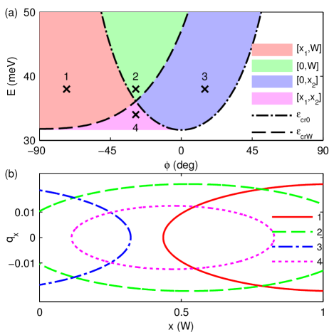
Figure 4: (a) The regions with different ranges of turning points for $W=200$ nm, $\Delta_{SO}=30$ meV, $\Delta=0$ and $B=0.2$ T. Different classically allowed trajectories are found in differently shaded regions, demarcated by the two critical boundaries. (b) A family of four different classical trajectories which correspond to the states labeled by numbered crosses in each region of (a).

In order to elucidate the quasi-classical behavior, in Fig. 4(a) we plot the zones corresponding to different configurations of turning points by different colors. The same set of parameters is used as in Fig. 3(e) ($\Delta_{SO}=30$ meV, $W=200$ nm, $B=0.2$ T and $s=+1$). In Fig. 4(b) we plot a set of classical trajectories that correspond to the zones shown in Fig. 4(a). As could be inferred from Fig. 2, for $\epsilon$ larger than both $\epsilon_{cr0}$ and $\epsilon_{crW}$ (green colored region in Fig. 4(a)), there is no classically forbidden region inside the barrier. However, if the electron energy is between the two critical energies (red or blue colored region in Fig. 4(a)), a classically forbidden energy range will appear on either end of the barrier. In other words, the electron will have to tunnel through a part of the barrier adjacent to one of its interfaces, whereas propagation is free in the other part. For the most extreme case displayed as the magenta colored region in Fig. 4(a), the electron has to tunnel through both ends of the barrier.

One may notice that the two critical energies whose variation with $\phi$ is depicted by dash-dotted and dotted lines in Fig. 3 are almost identical for the two spins. Also, by careful inspection of Fig. 3 it becomes evident that the quasi-classical zones we derived explain the observed transmission very well, especially for the spin up states. For the spin down states, however, transmission is enhanced with respect to the spin up states in the zones for which the electron waves must tunnel through a region of the barrier (the red and blue energy zones in Fig. 4(a)). This could be understood if one recalls that the WKB expression for the tunneling coefficient is given by

$$T\approx e^{-2Im\int q_{x}\left(x\right)dx},$$ (28)

where the integration is over a classically forbidden region. Having this in mind, it is obvious that for $\Delta_{SOC}\neq 0$ and $B\neq 0$ spin-up states decay faster than the spin-down states in classically forbidden regions, due to the paramagnetic term. This difference increases at higher magnetic fields, which leads to an increasing difference between the transmission coefficients for the two spins, as Fig. 3 clearly demonstrates. When the magnetic field is absent, the emerging paramagnetism vanishes, and therefore, the transmission characteristics for the two spins are identical (see Figs. 3(a) and (b)).

Next, we explore how the presence of the magnetic moments affects the interference pattern shown in Fig. 3. This could be the most important effect from a practical point of view. In the Fabry-Perot model, the interference pattern depends on the phase the electron wave function accumulates between the barrier interfaces and the bounces from the interface(s) and/or turning point(s)

$$\alpha=\alpha_{WKB}+\alpha_{1}+\alpha_{2},$$ (29)

where $\alpha_{1}$ and $\alpha_{2}$ are the backreflection phases, whereas $\alpha_{WKB}$ is the WKB phase

$$\alpha_{WKB}=2\int_{\max\left(0,x_{1}\right)}^{\min\left(W,x_{2}\right)}q_{x}\left(x\right)dx.$$ (30)

To analyze how the orbital magnetic moments influence the fringe pattern we could once again invoke Eq. (20) and the associated diagram in Fig. 4. It follows that Fabry-Perot resonances have different character in the different zones. Whenever $B\neq 0$, the WKB phase is accumulated throughout the entire barrier for $\epsilon>\max\left(\epsilon_{cr0},\epsilon_{crW}\right)$, but only in region $\left[x_{1},W\right]$ for $\epsilon_{cr0}>\epsilon>\epsilon_{crW}$ (the red-shaded region in Fig. 4(a)). Consequently, in the latter case the transmission maxima (depicted by the red color in Fig. 3) are almost linear functions of $\phi$, whereas in the former case their dependence on $\phi$ is nonlinear.

The crucial point, however, is that the phase accumulated during the propagation differs for the different spin orientations. This occurs because magnetic moments associated with opposite spins contribute to $\alpha_{WKB}$ in opposite ways (see Eq. (20)). To see this clearly, and to provide experimentally verifiable predictions it is important to consider the conductivity of the entire studied structure, given as,masir09

$$G\left(\epsilon\right)=G_{0}\int_{-\pi/2}^{\pi/2}T\left(\epsilon,\phi\right)\epsilon\cos\phi d\phi,$$ (31)

where $G_{0}=e^{2}L/2\hbar\pi^{2}$, with $L$ denoting the lateral width of the entire structure in the $y$ direction.

Figure 5: The derivative of the conductance versus incident energy, for (a) $0.1$ T, (b) $0.2$ T and (c) $0.3$ T. All other parameters are the same as in Fig. 3. Insets show the variation of the conductance with incident energy for the corresponding magnetic field.

Since the effects of magnetic moments are most vividly manifested in the dependence of $dG/dE$ on energy, we display this quantity in Fig. 5, for the same set of parameters as in Fig. 3. Alongside with $dG/dE$, the corresponding conductance is shown in the insets for each case. As can be seen from these insets, $G$ only depicts the fact that the spin-down conductance is increased with respect to the spin-up conductance, due to the enhanced transmission through the classically forbidden regions, as already discussed. On the other hand, the first derivative of the conductance with respect to energy conveys the information of the interference pattern, where the effects of the orbital moments are more transparent. Two issues are of importance here: (i) The difference between the two spins is clearly more pronounced at higher magnetic fields. This happens because in such a case the orbital moments have a larger impact on the electron dynamics, as pointed out before. (ii) The distinction between the two spins is more prominent at lower energies. This is a consequence of the larger emerging orbital magnetic moments of the electrons whose energies are close to the band edges than of more energetic electrons, as Eq. (4) and Fig. 1(a) demonstrate.

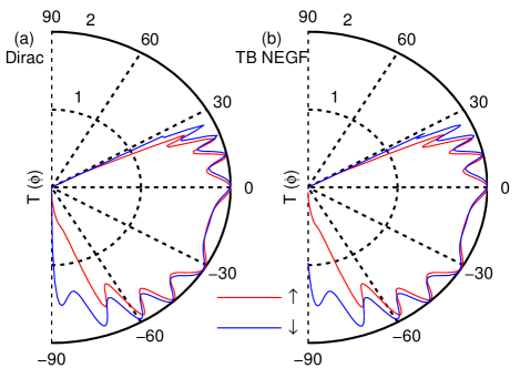
Figure 6: Transmission curves calculated using (a) the continuum and (b) the TB NEGF method. The parameters are $W=200$ nm, $B=0.3$ T and $E=100$ meV.

Finally, we would like to point out that the manifestation of orbital moments in transport properties can be captured by the tight-binding nonequilibrium Green function formalism as well. To show this, in Fig. 6(a) we plot a set of transmission curves obtained using the derived transmission amplitude, while in Fig. 6(b) we plot the results of our numerical transport simulations within the TB NEGF method, for the same barrier parameters. The phenomenological model used to describe graphene in this case is given by

$$H=-t\sum_{\langle i,j\rangle,\alpha}e^{i\varphi_{ij}}c^{\dagger}_{i\alpha}c_{j\alpha}+i\lambda_{SO}\sum_{\langle\langle i,j\rangle\rangle,\alpha,\beta}\nu_{ij}e^{i\varphi_{ij}}c^{\dagger}_{i\alpha}s^{z}_{\alpha\beta}c_{j\beta}.$$ (32)

The first term describes the usual hopping between nearest neighbor $p_{z}$ orbitals in graphene, which extends beyond the barrier. The second term describes the intrinsic spin-orbit interaction found in the barrier, through the next-nearest-neighbor (NNN) hopping amplitude $\lambda_{SO}$ ($\Delta_{SO}=3\sqrt{3}\lambda_{SO}$). Note that $\nu_{ij}$ determines the sign of the hopping; it is positive (negative) if an electron makes a right (left) turn at the intermediate atom in hopping from site $j$ to site $i$. The Peierls term $\varphi_{ij}=\frac{e}{\hbar}\int_{\mathbf{r_{i}}}^{\mathbf{r_{j}}}\mathbf{A}\cdot d\mathbf{l}$ accounts for the phase the electron acquires while traveling in the presence of the magnetic field. The details of the NEGF procedure can be found in Refs.  li08, ; datta95, ; futnota, ; liu12, .

Although the continuum and the TB NEGF schemes differ substantially as far as the formalism and implementation are concerned, they give practically indistinguishable results. This is not surprising, having in mind that the continuum Dirac picture is the effective theory corresponding to the low energy tight-binding method. Therefore, both approaches display these Zeeman-type effects, even though we use only minimal coupling and the Peierls substitution, to account for the influence of the magnetic field. Since strain in honeycomb lattices effectively induces time-reversal invariant pseudomagnetic fields,guinea10 stretching of insulating Dirac monolayers will inevitable galvanize orbital moments as well.grujic14

Note that the TB NEGF method could prove handy for studying the effects of disorder and imperfections on the manifestation of the spin-contrasting orbital moments. However, unlike the orbital moments coupled to the spin, the valley-contrasting orbital moments can not be distinguished by the TB NEGF transport simulations, since the contributions from the two valleys are inherently summed together, and cannot be separated. In this case, only the continuum calculations, where the valley degree of freedom is explicit, can elucidate the underlying physics.

V Conclusion

In this paper, we addressed the orbital magnetic moments emerging from the topology of insulating Dirac systems, as well as their manifestation on transport characteristics. In particular, we first closely examined the moments coupled to the spin degree of freedom, arising due to strong spin-orbit coupling, and thus leading to the renormalization of the g-factor. Their duality with the valley-contrasting orbital moments found in honeycomb lattices with broken spatial symmetry is reviewed, alongside with the duality of the Landau spectrum, particularly manifested in the behavior of the zeroth Landau level.

After establishing that magnetic properties couple with $\Delta_{SO}$ and the spin quantum number on the one hand, and $\Delta$ and the valley quantum number on the other hand in an analogous fashion, we go on to explore the influence of the orbital magnetic moments on the transport properties. In particular, we focused on the transmission through a single 1D barrier made of artificially enhanced spin-orbit coupling in graphene. We have shown that certain Zeeman-like magneto-transport signatures are a clear manifestation of the induced moments. The conductance $G$ through the device for the two spins start deviating from each other with increasing magnetic field. The effects of the moments on the fringe pattern of the transmission coefficients are most clearly observed in the energy dependence of the derivative of the conductance with respect to the electron energy $dG/dE$. This quantity reflects the increasing shifts in the interference maxima of opposite spins with increasing magnetic field; they are largest near the band edges, and they decrease for larger energies due to the decrease of the orbital magnetic moments themselves.

Because of the analogy between the mass and the SOC terms and the orbital moments they induce, the results presented here are also valid for valley transmission through a barrier with only $\Delta\neq 0$. This, however, can not be captured by numerical techniques such as the TB NEGF method, which is only able to account for the spin degree of freedom, and the associated orbital moments. Nevertheless, this behavior should be present in real devices, even in the absence of a clearly observable transport gap, since the Berry curvature hot spot can extend over a wide energy range.

Appendix A Transmission through a barrier in bulk graphene

The studied structure and the chosen gauge for the vector potential (Eq. (18)) ensure translational invariance along the $y$ direction, so $k_{y}$ is a good quantum number and the solutions have the form $\Psi(x,y)=\exp(ik_{y}y)\left(\psi_{A}(x),\psi_{B}(x)\right)^{T}$. The following coupled system of differential equations, for the amplitudes on the two sublattices can then be obtained:

$$\left(\tau k_{x}\mp ik_{y}\mp i\frac{e}{\hbar}A_{y}\right)\psi_{B/A}\pm\delta\psi_{A/B}=\epsilon\psi_{A/B}.$$ (33)

Reducing the coupled system to a set of two independent second order differential equations leads to

$$\left[\partial_{x}^{2}\mp\tau\frac{e}{\hbar}(\partial_{x}A_{y})-(k_{y}+\frac{e}{\hbar}A_{y})^{2}+\epsilon^{2}-\delta^{2}\right]\psi_{A/B}=0.$$ (34)

Having in mind the form of the vector potential, the differential equation in the barrier becomes

$$\left[\partial_{x}^{2}\mp\frac{\tau}{l_{B}^{2}}-(k_{y}+\frac{x}{l_{B}^{2}})^{2}+\epsilon^{2}-\delta^{2}\right]\psi_{A/B}=0.$$ (35)

By using the transformation $z=\sqrt{2}\left(k_{y}l_{B}+x/l_{B}\right)$ the following equation is obtained

$$\left[\partial_{z}^{2}+1/2-1/2\mp\tau\frac{1}{2}+\left(\epsilon^{2}-\delta^{2}\right)\frac{l_{B}^{2}}{2}-\frac{z^{2}}{4}\right]\psi_{A/B}=0,$$ (36)

which is of the form of the parabolic cylinder (Webers) differential equation

$$y^{\prime\prime}+\left(\nu+\frac{1}{2}-\frac{z^{2}}{4}\right)y=0,$$ (37)

whose solutions are given in terms of parabolic cylinder functions

$$y=C_{1}D_{\nu}(z)+C_{2}D_{\nu}(-z).$$ (38)

Finally the solution for the first sublattice is given by

$$\begin{split}\psi_{A}=&C_{1}D_{\nu_{A}}\left[\sqrt{2}\left(k_{y}l_{B}+x/l_{B}\right)\right]\\ +&C_{2}D_{\nu_{A}}\left[-\sqrt{2}\left(k_{y}l_{B}+x/l_{B}\right)\right],\end{split}$$ (39)

where $\nu_{A}=\left(\epsilon^{2}-\delta^{2}\right)l_{B}^{2}/2-\tau/2-1/2$. For the other sublattice after employing the recurrence relations

$$\frac{\partial D_{\nu}(z)}{\partial_{z}}=\frac{1}{2}zD_{\nu}(z)-D_{\nu+1}(z),$$ (40)

and the relationship (33), one obtains the following expression

$$\begin{split}\psi_{B}=&C_{1}gD_{\nu_{B}}\left[\sqrt{2}\left(k_{y}l_{B}+x/l_{B}\right)\right]\\ -&C_{2}gD_{\nu_{B}}\left[-\sqrt{2}\left(k_{y}l_{B}+x/l_{B}\right)\right],\end{split}$$ (41)

where $\nu_{B}=\left(\epsilon^{2}-\delta^{2}\right)l_{B}^{2}/2+\tau/2-1/2$, and

$$g=i\left[\frac{\sqrt{2}}{\left(\epsilon+\tau\delta\right)l_{B}}\right]^{\tau}.$$ (42)

If the relation

$$D_{\nu}\left(z\right)=2^{-\nu/2}e^{-z^{2}/4}H_{\nu}\left(\frac{z}{\sqrt{2}}\right)$$ (43)

is employed, the spinor multiplied by $C_{1}$ in Eqs. (39) and (41) reduces to the solution (12), once the incident energy is equal to a particular Landau level, as could be expected.

The incident wave function is given by

$$\psi_{I}=e^{ik_{x}x}\left(\begin{array}[]{c}1\\ \tau e^{i\tau\phi}\end{array}\right)+re^{-ik_{x}x}\left(\begin{array}[]{c}1\\ \tau e^{i\tau(\pi-\phi)}\end{array}\right),$$ (44)

where $\phi=\arctan k_{y}/k_{x}$.

Finally, in the third region the vector potential is a non-zero constant, and employing the standard plane wave ansatz, the solution is given by

$$\psi_{III}=t\sqrt{\frac{k_{x}}{k_{x}^{\prime}}}e^{ik_{x}^{\prime}x}\left(\begin{array}[]{c}1\\ \tau e^{i\tau\theta}\end{array}\right),$$ (45)

with the energy of the plane wave given by $\epsilon=\alpha\sqrt{k_{x}^{\prime 2}+k_{y}^{\prime 2}}$, $k_{x}^{\prime}=\epsilon\cos\theta$, the effective transverse momentum after the barrier $k_{y}^{\prime}=\epsilon\sin\theta=k_{y}+W/l_{B}^{2}$ and $\theta$ being the angle of energy propagation, with respect to the direction transverse to the barrier. The additional factor under the square root follows from current conservation.allain11 Again by replacing the expression for the momenta before and after the barrier, one obtains the effective law of refraction for a barrier of thickness $W$ with nonzero $\Delta$, $\Delta_{SO}$ and $B$ as

$$\epsilon\sin\theta=\epsilon\sin\phi+W/l_{B}^{2}.$$ (46)

The expressions for the wavefunctions in different regions, (44), (39), (41), and (45) are then matched at the interfaces $x=0$ and $x=W$, which gives a system of equations, whose solution yields the transmission amplitude $t$

$$t=\frac{2g\tau\cos(\tau\phi)\left(G_{A}^{+}G_{B}^{-}+G_{A}^{-}G_{B}^{+}\right)}{e^{ik_{x}^{\prime}W}f}\sqrt{\frac{k_{x}^{\prime}}{k_{x}}},$$ (47)

where

$$\begin{split}f=g^{2}\left(F_{B}^{+}G_{B}^{-}-F_{B}^{-}G_{B}^{+}\right)+e^{i\tau\left(\theta-\phi\right)}\left(F_{A}^{+}G_{A}^{-}-F_{A}^{-}G_{A}^{+}\right)\\ +g\tau e^{i\tau\theta}\left(F_{B}^{-}G_{A}^{+}+F_{B}^{+}G_{A}^{-}\right)+g\tau e^{-i\tau\phi}\left(F_{A}^{+}G_{B}^{-}+F_{A}^{-}G_{B}^{+}\right).\end{split}$$ (48)

Here the coefficients $F^{\pm}$ and $G^{\pm}$ are given by

$$F^{\pm}_{A/B} =D_{\nu_{A/B}}\left[\pm\sqrt{2}k_{y}l_{B}\right],$$ (49)

$$G^{\pm}_{A/B} =D_{\nu_{A/B}}\left[\pm\sqrt{2}(k_{y}l_{B}+\frac{W}{l_{B}})\right].$$ (50)

References

- (1) B. Hunt, J. D. Sanchez-Yamagishi, A. F. Young, M. Yankowitz, B. J. LeRoy, K. Watanabe, T. Taniguchi, P. Moon, M. Koshino, P. Jarillo-Herrero, and R. C. Ashoori, Science 340, 1427 (2013).
- (2) C. R.Woods, L. Britnell, A. Eckmann, R. S. Ma, J. C. Lu, H. M. Guo, X. Lin, G. L. Yu, Y. Cao, R. V. Gorbachev, A. V. Kretinin, J. Park, L. A. Ponomarenko, M. I. Katsnelson, Yu. N. Gornostyrev, K.Watanabe, T. Taniguchi, C. Casiraghi, H-J. Gao, A. K. Geim, and K. S. Novoselov, Nat. Phys. 10, 451 (2014).
- (3) J. Jung, A. DaSilva, S. Adam, and A. H. MacDonald, arXiv:1403.0496v1.
- (4) A. H. Castro Neto and F. Guinea, Phys. Rev. Lett. 103, 026804 (2009).
- (5) O. Shevtsov, P. Carmier, C. Groth, X. Waintal, and D. Carpentier, Phys. Rev. B 85, 245441 (2012).
- (6) H. Jiang, Z. Qiao, H. Liu, J. Shi, and Q. Niu, Phys. Rev. Lett. 109, 116803 (2012).
- (7) J. Balakrishnan, G. K. Koon, M. Jaiswal, A. H. Castro Neto, and B. Ozyilmaz, Nat. Phys. 9, 284 (2013).
- (8) A. Avsar, J. Y. Tan, T. Taychatanapat, J. Balakrishnan, G.K.W. Koon, Y. Yeo, J. Lahiri, A. Carvalho, A. S. Rodin, E.C.T. O’Farrell, G. Eda, A. H. Castro Neto, and B. Ozyilmaz, Nat. Commun. 5, 4875 (2014).
- (9) C.-C. Liu, W. Feng, and Y. Yao, Phys. Rev. Lett. 107, 076802 (2011).
- (10) S. Cahangirov, M. Topsakal, E. Aktürk, H. Şahin, and S. Ciraci, Phys. Rev. Lett. 102, 236804 (2009).
- (11) Y. Xu, B. Yan, H. J. Zhang, J. Wang, G. Xu, P. Tang, W. Duan, and S. C. Zhang, Phys. Rev. Lett. 111, 136804 (2013).
- (12) also gives rise to massive particles, by virtue of opening the gap, however for brevity we refer only to the term as mass.
- (13) C. L. Kane and E. J. Mele, Phys. Rev. Lett. 95, 146802 (2005).
- (14) M.-C. Chang and Q. Niu, Phys. Rev. B 53, 7010 (1996).
- (15) D. Xiao, W. Yao and Q. Niu, Phys. Rev. Lett. 99, 236809 (2007).
- (16) K. F. Mak, K. L. McGill, J. Park, and P. L. McEuen, Science 344, 1489 (2014).
- (17) R. V. Gorbachev, J. C. W. Song, G. L. Yu, A. V. Kretinin, F. Withers, Y. Cao, A. Mishchenko, I. V. Grigorieva, K. S. Novoselov, L. S. Levitov, and A. K. Geim, Science 346, 448 (2014).
- (18) W. Feng, Y. Yao, W. Zhu, J. Zhou, W. Yao, and D. Xiao, Phys. Rev. B 86, 165108 (2012).
- (19) D. Xiao, G. B. Liu, W. Feng, X. Xu, and W. Yao, Phys. Rev. Lett. 108, 196802 (2012).
- (20) M. M. Grujić, M. Ž. Tadić, and F. M. Peeters, Phys. Rev. Lett. 113, 046601 (2014).
- (21) F. Zhang, J. Jung, G. A. Fiete, Q. Niu, and A. H. MacDonald, Phys. Rev. Lett. 106, 156801 (2011).
- (22) H. Min, G. Borghi, M. Polini, and A. H. MacDonald, Phys. Rev. B 77, 041407 (2008).
- (23) F. Zhang, H. Min, M. Polini, and A. H. MacDonald, Phys. Rev. B 81, 041402 (2010).
- (24) R. Nandkishore and L. Levitov, Phys. Rev. B 82, 115124 (2010).
- (25) J. Jung, F. Zhang, and A. H. MacDonald, Phys. Rev. B 83, 115408 (2011).
- (26) C. L. Kane and E. J. Mele, Phys. Rev. Lett. 95, 226801 (2005).
- (27) W. Yao, D. Xiao, and Q. Niu, Phys. Rev. B 77, 235406 (2008).
- (28) D. Xiao, M. C. Chang, and Q. Niu, Rev. Mod. Phys. 82, 1959 (2010).
- (29) M. C. Chang and Q. Niu, J. Phys.: Condens. Matter 20, 193202 (2008).
- (30) M. Gradhand, D. V. Fedorov, F. Pientka, P. Zahn, I. Mertig, and B. L. Györffy, J. Phys.: Condens. Matter 24, 213202 (2012).
- (31) F. D. M. Haldane, Phys. Rev. Lett. 61, 2015 (1988).
- (32) M. Ezawa, Phys. Rev. B 86, 161407 (2012).
- (33) A. Kormányos, V. Zólyomi, N. D. Drummond, and G. Burkard, Phys. Rev. X 4, 011034 (2014).
- (34) C. J. Tabert and E. J. Nicol, Phys. Rev. Lett. 110, 197402 (2013).
- (35) P. M. Ostrovsky, I. V. Gornyi, and A. D. Mirlin, Phys. Rev. B 77, 195430 (2008).
- (36) P. M. Krstajić and P. Vasilopoulos, Phys. Rev. B 86, 115432 (2012).
- (37) J. L. Lado, J. W. González, and J. Fernández-Rossier, Phys. Rev. B 88, 035448 (2013).
- (38) M. Ezawa, Phys. Rev. Lett. 109, 055502 (2012).
- (39) X. Li, F. Zhang, and Q. Niu, Phys. Rev. Lett. 110, 066803 (2013).
- (40) T. Cai, S. A. Yang, X. Li, F. Zhang, J. Shi, W. Yao, and Q. Niu, Phys. Rev. B 88, 115140 (2013).
- (41) M. Koshino and T. Ando, Phys. Rev. B 81, 195431 (2010).
- (42) M. O. Goerbig, Rev. Mod. Phys. 83, 1193 (2011).
- (43) M. Grujić, M. Zarenia, A. Chaves, M. Tadić, G. A. Farias, and F. M. Peeters, Phys. Rev. B 84, 205441 (2011).
- (44) L. Majidi and M. Zareyan, Phys. Rev. B 83, 115422 (2011).
- (45) M. Ramezani Masir, P. Vasilopoulos, A. Matulis, and F. M. Peeters, Phys. Rev. B 77, 235443 (2008).
- (46) M. Ramezani Masir, P. Vasilopoulos, and F. M. Peeters, Phys. Rev. B 79, 035409 (2009).
- (47) T. C. Li and S.-P. Lu, Phys. Rev. B 77, 085408 (2008).
- (48) S. Datta, Electronic Transport in Mesoscopic Systems (Cambridge University Press, Cambridge, 1995).
- (49) In order to compare the results with the continuum theory, we need the numerical simulations within the NEGF formalism to provide us with the angular dependence of the transmission through a structure infinite in the -direction. To achieve this, we resort to the recipe described in Ref. liu12, . In short, we take the narrowest possible zigzag nanoribbon, placed along the -direction, where the semi-infinite left and right leads surround the barrier region in which SOC NNN hopping is nonzero. The structure is then taken to be periodic along the -direction, prompting the use of the Bloch theorem in this direction. This means that the phase factor will enter all hopping terms along the axis, which is none other than the transverse momentum . In this way, appears as a parameter, and since the incident energy is a parameter as well, one is then able to reconstruct the angle of propagation using . Note that in our case, besides the Peierls phase factor, we must also add the vector potential, Eq. (18), to , in order to properly model the influence of the magnetic field. Finally, one needs to connect the Fermi velocity entering the Dirac equation, with the nearest-neighbor hopping , as , where nm is the carbon-carbon distance, and the hopping is set to eV.
- (50) M. H. Liu, J. Bundesmann, and K. Richter, Phys. Rev. B 85, 085406 (2012).
- (51) F. Guinea, M. I. Katsnelson, and A. K. Geim, Nat. Phys. 6, 30 (2010).
- (52) P. E. Allain and J. N. Fuchs, Eur. Phys. J. B 83, 301 (2011).