Self-assembly of hard helices: a rich and unconventional polymorphism

Abstract

Hard helices can be regarded as a paradigmatic elementary model for a number of natural and synthetic soft matter systems, all featuring the helix as their basic structural unit: from natural polynucleotides and polypeptides to synthetic helical polymers; from bacterial flagella to colloidal helices. Here we present an extensive investigation of the phase diagram of hard helices using a variety of methods. Isobaric Monte Carlo numerical simulations are used to trace the phase diagram: on going from the low-density isotropic to the high-density compact phases, a rich polymorphism is observed exhibiting a special chiral screw-like nematic phase and a number of chiral and/or polar smectic phases. We present a full characterization of the latter, showing that they have unconventional features, ascribable to the helical shape of the constituent particles. Equal area construction is used to locate the isotropic–to–nematic phase transition, and results are compared with those stemming from an Onsager-like theory. Density functional theory is also used to study the nematic–to–screw-nematic phase transition: within the simplifying assumption of perfectly parallel helices, we compare different levels of approximation, that is second- and third-virial expansions and Parsons-Lee correction.

I Introduction

Short-range repulsive interactions are those mainly responsible for the structure of classical particle fluid systems; this is what originally conferred worthiness to hard–body particle models.Barker76 These have actually proven to be a very good representation of colloidal particle systems, with a very good agreement between the theoretical phase diagram of hard spheres and the experimental phase behaviour of colloidal spheres.Pusey86 Today, ever-increasing importance of colloids and advances in the synthesis of colloidal particles of non-spherical symmetry Glotzer07 ; Sacanna13a ; Sacanna13b are depriving theoretical studies of any hard particle system of what is remaining of a mere academic aura, demonstrating that these studies may be crucial for the design of new colloidal materials.Solomon11

Helical particles are especially worth investigating as Nature has conferred to the helix a rather prominent role. Helical polynucleotides and polypeptides function at large enough densities that the details of their shape start to be relevant.Stevens14 The desire of mimicking Nature in reproducing the functions carried out by helical biopolymers has, in turn, led to a very active area in polymer research – the synthesis and characterisation of helical polymers, aiming at exploiting the inherent chirality of the helical structure to produce new functional materials to be used especially in asymmetric catalysis and enantiomeric separation. Nakano01 ; Yashima09

This material interest merges with its inherent biological interest in the currently pursued attempt to employ DNA, perhaps the most emblematic of all helical biomolecular systems, as a building-block for new materials.Seeman03 ; Douglas09

Rather surprisingly, in spite of this wealth of inspiration sources, helices appear to have been mostly overlooked in past theoretical studies on hard-body non-spherical particle systems, focussing mostly on rod- or disc-like particles,Allen93 ; Tarazona08 possibly due to the tacit assumption that helices, as elongated objects, can be assimilated to rods.

To fill this gap, we have undertaken a systematic investigation of the phase behaviour of hard helices, using numerical simulation and density functional theory. We have found how finely the isotropic–nematic phase boundaries depend on the structural parameters defining a helical particle, with a dependence not simply rooted in its aspect ratio, thus making a mapping onto an effective rod rather loose.Frezza13 More importantly, we have also provided evidence for the existence of a new chiral nematic phase, named screw-nematic, the helix twofold symmetry axes spiral around the main phase director.Kolli14 This was the phase observed in experiments on systems of colloidal helical filaments,Barry06 but our results on such a basic model suggest this screw-nematic phase to be a general feature of any helical particle system, including DNA suspensions at sufficiently high densities.Manna07

In the present work, we build upon past work by extending it in several respects. (i) We present a complete phase diagram in the density-pressure plane, with a special emphasis on the smectic phases occurring at densities higher than those typical of the conventional and screw-nematic phases, and discuss how the screw-nematic order merges with a tendency to layering to produce new chiral, screw-like, smectic phases. (ii) We perform a detailed study of the isotropic–nematic coexistence; (iii) We extend the second-virial theory for the nematic–to–screw-nematic phase transition Kolli14 by adding the third-virial contribution, and validate it against numerical simulations.

In the next section, we provide details on the various theoretical and computational methods used. We first describe the Monte Carlo simulation technique and then the density functional theory at different levels of approximation. Section III presents and discusses the results, sub-divided in several parts. In the first, phase diagrams, as obtained from isobaric Monte Carlo simulations, are shown and the structure of the smectic phases occurring in the higher density regions is described by means of positional and orientational order parameters and pair correlation functions. In the second part, attention is paid to the isotropic–nematic phase transition, with the aim of a proper location of the coexisting densities and pressure. The third part presents the theoretical results for the nematic–to–screw-nematic phase transition. Finally, Section IV concludes this work by giving a brief summary and possible outlooks.

II Model and Methods

Helices were simply modelled as a line of 15 fused hard spherical beads of diameter $D$ rigidly arranged into a helicoidal shape, with a contour length fixed to $L=10D$.Frezza13 On changing the radius $r$ and pitch $p$ at fixed $L$, the shape of the helical particle can be tuned from a straight rod to very wound coils (Fig.1).

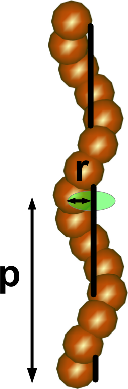
Figure 1: Model for a hard helix, with $r$ its radius and $p$ the pitch.

We focus on increasingly twisted helical shapes in the range $r/D\in[0.2;0.4]$ and $p/D\in[2;8]$. Such particles have a sufficiently large effective aspect ratio to display a rich polymorphic liquid-crystal phase behaviour, and yet they have an intermediate degree of ”curliness” ($L/p={\cal O}(1)$), so that phase sequences and phase structures are expected to depend sensitively on the overall set of parameters defining the particle shape. Hereafter, all lengths will be expressed in units of $D$.

To trace the full phase diagrams of such objects, we resorted to Monte Carlo (MC) numerical simulations in the isobaric(-isothermal) ensemble (MC-NPT) Allen87 ; Frenkel02 . These calculations were preceded by the construction of the initial compact configurations. Additional MC simulations in the canonical ensemble (MC-NVT) Allen87 ; Frenkel02 were performed in one specific case to identify the precise value of the volume fractions and pressure at the coexistence. Onsager theory, in different forms,Onsager49 ; Parsons79 ; Lee87 was used for studying the isotropic-to-nematic and nematic–screw-nematic phase transitions. The remainder of this section provides details on the various methods used to investigate the phase behaviour.

II.1 Isopointal search method (ISM)

One of the difficulties arising in simulations of non-spherical objects stems from the choice of a judicious set of initial conditions that allow a correct span of the whole phase diagram. Usually, a disordered initial condition is unable to probe the most compact phases. On the other hand, high-density compact configurations of particles of arbitrary shape are not readily envisageable and unexpected features may arise. In this respect, hard (sphero-)cylinders seem an exception;Bolhuis97 hard ellipsoids, thought for long to crystallise in a ”stretched-fcc” structure,Frenkel85 were recently shown to also do otherwise.Donev04 In order to cope with this problem, we have exploited an isopointal search method Hudson08 to construct compact configurations that we then used as initial configurations in most of the simulations. The method hinges on a structural search for dense packing, supported and guided by crystallographic inputs helping to reduce its computational cost, and coupled to an annealing scheme that progressively increases the density of a small number of helices within a unit cell, until the maximum possible packing is achieved.

Calculations were made for a single layer of parallel helices with their centres of mass lying on the same plane. This led to a considerable simplification in that one could limit the analysis to the $17$ two-dimensional wallpaper space groups, rather than having to deal with the full set of the $230$ three-dimensional space groups. When applied to a system of hard helices with radii ranging in the interval $0.1\leq r\leq 1$ and pitches in the range $1\leq p\leq 10$, the ISM predicts that, apart from the peculiar case of $p=1$, a specific wallpaper group with a single helix per unit cell provides the maximum possible packing fraction. Fig. 2 (bottom panel) provides a top view of the resulting structure in the case $r=0.2$ and $p=3$, with the circles having their centre coincident with the projection on a perpendicular plane to the helix axis, and their radius equal to the helix radius $r$ (the red circle) and to $r+1/2$ (the black circle). The black thick lines inside the red circles give the orientation of the twofold (C₂) symmetry axis of the helices. Notice that they are aligned along the same direction, meaning that helices are all in register. The darker grey areas indicate overlapping regions, where the grooves of neighbouring helices intrude into each other voids. For any given helix morphology, the method provides the shape and area of the unit cell, also displayed in Fig. 2.

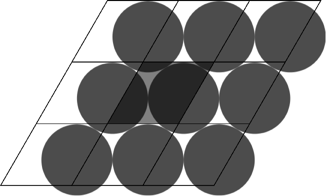
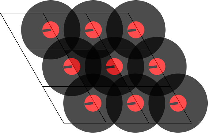
Figure 2: Maximally packed structure for two different cases. (Top) Non-overlapping circles, the two-dimensional counterpart of hard cylinders (limit case of helices with $r=0$ and $p=\infty$, having $\eta_{hex}=\pi/\sqrt{12}$). (Bottom) Overlapping circles corresponding to hard helices with $r=0.2$ and $p=3$.

The crucial quantity provided by the calculation is the ratio $A_{helix}/A_{cell}$ where $A_{helix}$ is the area occupied by the helix (i.e. the section of the cylinder containing the helix) and $A_{cell}$ the area of the unit cell. Because of the significant overlap between neighbouring helices, this ratio might exceed unity, as clearly indicated by the differences in the two pictures in Fig.2. In case of no overlap, the maximal packing would be the bidimensional hexagonal, having a packing fraction $\eta_{hex}=\pi/\sqrt{12}=0.9064\ldots$ and with each larger circle inscribed in the unit cell of area $A_{cell,hex}=(2r+1)^{2}\pi/3$ (Fig.2 top). This is significantly different from the reported example of a helix with $r=0.2$ and $p=3$ (Fig.2 bottom) where the black circle covers a surface substantially larger than the corresponding unit cell. The result for $A_{helix}/A_{cell}$ can then be translated into a volume fraction as

$$\eta = \frac{n_{helix}v_{0}}{A_{cell}\left(\Lambda+D\right)}$$ (1)

where $n_{helix}$ is the number of helices in the unit cell ($=1$ in the large majority of the cases, as anticipated), $v_{0}$ is the volume of the helix, calculated as in Ref.Frezza13 , and $\Lambda$ is the Euclidean length measured as the component parallel to the main axis of the helix of the distance between the first and the last bead.Frezza13 ; note3

The value of $\eta$ is reported in Fig. 3 in a colour map as a function of helix $r$ and $p$.

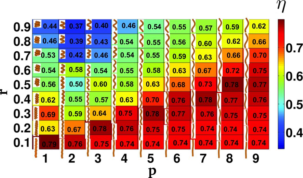
Figure 3: Colour map of the maximal packing fraction ($\eta$) as function of the helix $r$ and $p$. The digit inserts indicate the value of $\eta$. A snapshot of the correspoding helix is also shown in the inset.

Since these values for $\eta$ have been obtained by considering each layer as independent, they can only be regarded as a reasonable lower bound of the real maximally packed configuration that could be achieved by a further interlayer occupancy optimization. Yet, the so-built configurations constitute a very handy compact initial condition to achieve well equilibrated high density structures, as we will see below.

II.2 Isobaric Monte Carlo simulations

The MC-NPT method Wood68 was used for calculating the equation of state of a system of hard helical particles. Up to $N$=2000 particles were inserted in a generally triclinic and floppy (i.e. shape adapting) computational box, with standard periodic boundary conditions. Such conditions are fully appropriate as long as the spatial periodicity of the mesophases are comparable with the particle length scale, as it is the case of the various phases that we will be discussing in the present study. They would not be appropriate, however, for phases with a periodicity much longer than the particle size. This is in general the case of the cholesteric phase,Priestley74 ; deGennes93 which for this reason cannot be observed in our simulations. However, just because of its long length scale, the absence of the twist distortion is not expected to substantially affect the boundaries and the local structure of the nematic phase. For this reason, we will henceforth always refer to an untwisted conventional nematic phase, in spite of the chiral nature of helical particles. We will return to this point later on.

In the majority of cases, simulations were started from a compact configuration as generated by the ISM. Few tests were additionally carried out to check the robustness of the obtained results with respect to the choice of the initial conditions. Every simulation run was organised in cycles, each of them consisting of $N/2$ translational and $N/2$ rotational trial moves, performed either using quaternions or the Barker-Watts method Allen87 supplemented with a rotation around the helix main axis, and an attempt to vary shape and volume of the computational box. The typical length of the equilibration runs was $3-4\times 10^{6}$ MC cycles. Equilibration runs were then followed by typically $2\times 10^{6}$ MC cycle long production runs, during which averages of several order parameters and correlation functions were accumulated. These quantities were used to characterise and distinguish the various phases.

Dedicated additional simulations were also carried out with the helix long axes constrained along a fixed direction to validate the theory for the nematic–to–screw-nematic phase transition described in Section II.4.

II.3 Order parameters and correlation functions

Different liquid crystal phases will be distinguished by using appropriate order parameters combined with suitable correlation functions. For the definition of these quantities, we refer to Fig.4 where the helix main axis $\widehat{\mathbf{u}}$ and secondary axis $\widehat{\mathbf{w}}$, parallel to the C₂ symmetry axis, are shown, along with the unit vectors parallel to the main phase director ($\widehat{\mathbf{n}}$) and to the minor phase director ($\widehat{\mathbf{c}}$) at a given position. The various order parameters calculated are as follows.

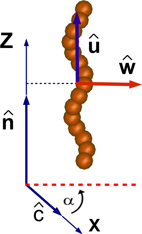
Figure 4: Helix with arrows showing the unit vectors $\widehat{\mathbf{u}}$ and $\widehat{\mathbf{w}}$ defined in the molecular frame, and the unit vectors $(\widehat{\mathbf{n}},\widehat{\mathbf{c}})$ defined in the laboratory frame. $X$, $Z$ are the axes of the laboratory frame, with $\alpha$ the angle between $\widehat{\mathbf{w}}$ and the $X$ axis.

• The nematic order parameter Priestley74 ; deGennes93 is defined as the averaged second Legendre polynomial

  $$\left\langle P_{2}\right\rangle = \left\langle\frac{3}{2}(\widehat{\mathbf{u}}\cdot\widehat{\mathbf{n}})^{2}-\frac{1}{2}\right\rangle,$$ (2)

  where the average is over the configurations. It can be computed using the standard procedure patterned after the early work of Veilliard-Baron Veilliard-Baron74 by introducing, for each configuration, the second-rank tensor

  $$Q_{\alpha\beta} = \frac{1}{N}\sum_{i=1}^{N}\frac{3}{2}\widehat{u}_{\alpha}^{i}\widehat{u}_{\beta}^{i}-\frac{1}{2}\delta_{\alpha\beta}$$ (3)

  with $\widehat{u}_{\alpha}$, $\widehat{u}_{\beta}$ the Cartesian components of $\widehat{\mathbf{u}}$ and $\delta_{\alpha,\beta}$ the Krönecker symbol. This second-rank traceless tensor is then diagonalized to compute the largest eigenvalue and the corresponding eigendirection. The latter is identified as the configuration’s nematic director $\widehat{\mathbf{n}}$. The maximum eigenvalues are then averaged over the configurations, to give the order parameter $\langle P_{2}\rangle$ defined in Eq.(2). This order parameter (essentially) vanishes in the isotropic phase (I) whereas in the nematic phase is (distinctly) larger than zero and approaches unity as density increases.

• The screw-nematic order parameter Kolli14 ; Manna07 is defined as

  $$\left\langle P_{1,c}\right\rangle = \left\langle\widehat{\mathbf{w}}\cdot\widehat{\mathbf{c}}\right\rangle.$$ (4)

  This order parameter measures the average alignment along a common direction ($\widehat{\mathbf{c}}$) of the secondary axes ($\widehat{\mathbf{w}}$) of helices having their centre of mass on the same plane perpendicular to the main director $\widehat{\mathbf{n}}$. In the screw-like organisation, the minor phase director $\widehat{\mathbf{c}}$, perpendicular to $\widehat{\mathbf{n}}$, rotates around it in a helical fashion with a pitch $p$. To determine this order parameter, we have followed the following procedure. Firstly for each configuration, after having determined the main director $\widehat{\mathbf{n}}$ as explained in the previous item, an untwisting of $-2\pi Z_{i}/p$ around $\widehat{\mathbf{n}}$ is enforced on the coordinates of particles, where $Z_{i}$ is the coordinate of the center mass of the $i$-th helix along the $Z$ axis parallel to $\widehat{\mathbf{n}}$. Then the quantity $\widehat{\mathbf{w}}\cdot\widehat{\mathbf{c}}$ is calculated for each helix and finally $\left\langle P_{1,c}\right\rangle$ is obtained by averaging over all helices and configurations. The order parameter $\left\langle P_{1,c}\right\rangle$ thus enables us to distinguish between the conventional (N) and the unconventional screw-nematic (N${}_{S}^{*}$) phases.

• The smectic order parameter Priestley74 ; deGennes93 is defined as

  $$\left\langle\tau_{1}\right\rangle = \left|\left\langle\mathsf{e}^{i2\pi\frac{\mathbf{R}\cdot\widehat{\mathbf{n}}}{d}}\right\rangle\right|,$$ (5)

  with $\mathbf{R}$ the position of a particle centre of mass and $d$ the optimal layer spacing. Evaluated following standard prescriptions (e.g. Ref.Memmer02 ; Cifelli06 ), $\langle\tau_{1}\rangle$ indicates the onset of a smectic phase, where particles tend to organise in layers perpendicular to the director $\widehat{\mathbf{n}}$.

• The sixfold bond-orientational (hexatic) order parameter and the average number of nearest-neighbours. The former order parameter is defined as:

  $$\left\langle\psi_{6}\right\rangle = \left\langle\frac{1}{N}\sum_{i=1}^{N}\left|\frac{1}{n(i)}\sum_{j=1}^{n(i)}e^{6\mathrm{i}\theta_{ij}}\right|\right\rangle.$$ (6)

  Here $\theta_{ij}$ is the angle that the $i$,$j$ intermolecular distance vector forms with a pre-fixed axis in a plane perpendicular to $\widehat{\mathbf{n}}$, while $n(i)$ is the number of nearest-neighbours of molecule $i$ within a single layer. As $\langle\tau_{1}\rangle$ can only signal the onset of a generic smectic phase, we will then be using $\langle\psi_{6}\rangle$ to probe the onset of hexatic order (e.g. Memmer02 ; Cinacchi08 ). The piece of information stemming from $\langle\psi_{6}\rangle$ can be supported by computing the average number $\langle n\rangle$ of nearest-neighbours within each layer, that tends to $6$ in the hexatic phase. This quantity is computed by averaging $n(i)$ over all helices in a plane, and over all possible configurations. We remark here that the actual value of $n(i)$ is rather sensitive to the definition of nearest-neighbours distance, that has always a certain degree of arbitrariness, especially for hard-body particles, and here is taken to be $1.1$. Both $\psi_{6}$ and $n(i)$ display consistent behaviour for different layers, and hence the results for a single, arbitraly chosen layer will be shown below.

In addition to order parameters, we have calculated several positional and orientational correlation functions that provide a more detailed picture of a single thermodynamic state point.

• The parallel positional correlation function:Cinacchi02

  $$g_{\|}(R_{\|}) = \frac{1}{N}\left\langle\frac{1}{\rho L_{x}L_{y}}\sum_{i=1}^{N}\sum_{j\neq i}^{N}\delta(R_{\|}-\mathbf{R}_{ij}\cdot\hat{\mathbf{n}})\right\rangle$$ (7)

• The perpendicular positional correlation function:Cinacchi02

  $$g_{\perp}(R_{\perp}) = \frac{1}{2\pi R_{\perp}N}\left\langle\frac{1}{\rho L_{z}}\sum_{i=1}^{N}\sum_{j\neq i}^{N}\delta\left(R_{\perp}-\left|\mathbf{R}_{ij}\times\hat{\mathbf{n}}\right|\right)\right\rangle$$

• The screw-like parallel orientational correlation function:Kolli14

  $$g_{1,\|}^{\widehat{\mathbf{w}}}(R_{\|}) = \left\langle\frac{\sum_{i=1}^{N}\sum_{j\neq i}^{N}\delta(R_{\|}-\mathbf{R}_{ij}\cdot\hat{\mathbf{n}})(\widehat{\mathbf{w}}_{i}\cdot\widehat{\mathbf{w}}_{j})}{\sum_{i=1}^{N}\sum_{j\neq i}^{N}\delta(R_{\|}-\mathbf{R}_{ij}\cdot\hat{\mathbf{n}})}\right\rangle.$$

  In Eqs. (7)-(LABEL:gw), $\rho=N/V$ is the number density of the system; $V$ is the volume of the sample; $L_{x}$ and $L_{y}$ are the computational box dimensions along mutually orthogonal directions normal to $\widehat{\mathbf{n}}$; $L_{z}$ is the computational box dimension along $\widehat{\mathbf{n}}$; $\delta()$ is the Dirac $\delta$-function and $\mathbf{R}_{ij}=\mathbf{R}_{j}-\mathbf{R}_{i}$ is the vector joining the centres of helices $i$ and $j$.

  The first two positional correlation functions, Eqs. (7) and (LABEL:gperp), are used to distinguish a homogeneous (isotropic or nematic) phase (both $g_{\|}(R_{\|})$ and $g_{\perp}(R_{\perp})$ liquid-like), a layered (smectic) phase ($g_{\|}(R_{\|})$ solid-like and $g_{\perp}(R_{\perp})$ liquid-like), a columnar phase ($g_{\|}(R_{\|})$ liquid-like and $g_{\perp}(R_{\perp})$ solid-like) or a crystalline phase (both $g_{\|}(R_{\|})$ and $g_{\perp}(R_{\perp})$ solid-like). Eq. (LABEL:gw) is used in connection with the screw-nematic order parameter, Eq. (4), for establishing and quantifying the existence of a screw-like type of order in the system.

II.4 Density Functional Theory (DFT)

This section describes the general density functional theory Wu07 framework that has been used for studying the I–N and the N–N${}^{*}_{S}$ phase transitions.

Let us consider a pure system of hard helices whose mechanical state is described by a set of translational and rotational variables. The former are collected under the symbol $\mathbf{R}$, while the latter under the symbol $\Omega$. The single–particle density function is then denoted as $\rho(\mathbf{R},\Omega)=\rho(\mathbf{x})$ and normalised such that $\int d\mathbf{x}\rho(\mathbf{x})=N$.

By retaining only the second and third terms in the virial expansion, the excess Helmholtz free energy of such a system is given by:

$$\beta\mathsf{F}^{ex} = \frac{1}{2}\int d\mathbf{x}d\mathbf{x}^{\prime}\rho(\mathbf{x})M(\mathbf{x},\mathbf{x}^{\prime})\rho(\mathbf{x}^{\prime})\left[1+\frac{1}{3}\int d\mathbf{x}^{\prime\prime}M(\mathbf{x},\mathbf{x}^{\prime\prime})\rho(\mathbf{x}^{\prime\prime})M(\mathbf{x}^{\prime\prime},\mathbf{x}^{\prime})\right],$$ (10)

with $\beta=1/k_{B}T$ and $M(\mathbf{x},\mathbf{x}^{\prime})$ the Mayer function changed in sign.McQuarrie00

Let us assume that the system can form liquid crystal phases and that the translational order, if any, is only present along one direction, $Z$, with a periodicity equal to $p$. Thus, the single-particle density function can be expressed as $\rho(\mathbf{x})=\rho(Z,\Omega)$. Therefore the excess free energy density of the system is given by:

$$\frac{\beta\mathsf{F}^{ex}}{V}=\beta\mathsf{f}^{ex}=\frac{1}{2p}\int_{0}^{p}dZd\Omega\rho(Z,\Omega)\int dZ^{\prime}d\Omega^{\prime}\rho(Z^{\prime},\Omega^{\prime})\biggl{[}a_{excl}(Z,\Omega,Z^{\prime},\Omega^{\prime})+\frac{1}{3}\int dZ^{\prime\prime}d\Omega^{\prime\prime}\rho(Z^{\prime\prime},\Omega^{\prime\prime})a_{3}(Z,\Omega,Z^{\prime},\Omega^{\prime},Z^{\prime\prime},\Omega^{\prime\prime})\biggr{]},$$

(11)

where the functions $a_{excl}(Z,\Omega,Z^{\prime},\Omega^{\prime})$ and $a_{3}(Z,\Omega,Z^{\prime},\Omega^{\prime},Z^{\prime\prime},\Omega^{\prime\prime})$ have been introduced. The first is given by:

$$a_{excl}(Z,\Omega,Z^{\prime},\Omega^{\prime})=\int\int dX^{\prime}dY^{\prime}M(0,Z,\Omega,X^{\prime},Y^{\prime},Z^{\prime},\Omega^{\prime})$$ (12)

and is interpreted as the area of the surface obtained by cutting with a plane perpendicular to the director and at position $Z^{\prime}$ the volume excluded to a particle with orientation $\Omega^{\prime}$ by a particle at position $Z$ and with orientation $\Omega$.Cinacchi04 The second function in eq.11 is given by:

$$a_{3}(Z,\Omega,Z^{\prime},\Omega^{\prime},Z^{\prime\prime},\Omega^{\prime\prime})=$$

$$\int dX^{\prime}dY^{\prime}dX^{\prime\prime}dY^{\prime\prime}M(0,Z,\Omega,X^{\prime},Y^{\prime},Z^{\prime},\Omega^{\prime})M(0,Z,\Omega,X^{\prime\prime},Y^{\prime\prime},Z^{\prime\prime},\Omega^{\prime\prime})M(X^{\prime},Y^{\prime},Z^{\prime},\Omega^{\prime},X^{\prime\prime},Y^{\prime\prime},Z^{\prime\prime},\Omega^{\prime\prime}),$$

but does not lend itself to a ready geometrical interpretation. Since $a_{excl}$ and $a_{3}$ actually depend on the differences $\zeta^{\prime}=Z^{\prime}-Z$ and $\zeta^{\prime\prime}=Z^{\prime\prime}-Z$, the equation above can be re-written in a slightly neater way as:

$$\frac{\beta\mathsf{F}^{ex}}{V}=\beta\mathsf{f}^{ex}=\frac{1}{2p}\int_{0}^{p}dZd\Omega\rho(Z,\Omega)\int d\zeta^{\prime}d\Omega^{\prime}\rho(Z+\zeta^{\prime},\Omega^{\prime})\biggl{[}a_{excl}(\Omega,\zeta^{\prime},\Omega^{\prime})+\frac{1}{3}\int d\zeta^{\prime\prime}d\Omega^{\prime\prime}\rho(Z+\zeta^{\prime\prime},\Omega^{\prime\prime})a_{3}(\zeta^{\prime},\Omega,\Omega^{\prime},\zeta^{\prime\prime},\Omega^{\prime\prime})\biggr{]}$$

(13)

The single-particle density function can be decomposed as follows:

$$\rho(Z,\Omega)=\rho(Z)f(\Omega|Z),$$ (14)

with $\rho(Z)$ the purely translational single particle density, normalised such that $(1/p)\int_{0}^{p}dZ\rho(Z)=\rho$, and $f(\Omega|Z)$ the particle orientational distribution function at position $Z$, normalised such that $\int d\Omega f(\Omega|Z)=1$, irrespective of $Z$. Thus:

$$\frac{\beta\mathsf{F}^{ex}}{V} = \beta\mathsf{f}^{ex}=\frac{1}{2p}\int_{0}^{p}dZ\rho(Z)\int d\Omega f(\Omega|Z)\int d\zeta^{\prime}\rho(Z+\zeta^{\prime})\int d\Omega^{\prime}f(\Omega^{\prime}|Z+\zeta^{\prime})$$ (15)

$$\biggl{[}a_{excl}(\Omega,\zeta^{\prime},\Omega^{\prime})+\frac{1}{3}\int d\zeta^{\prime\prime}\rho(Z+\zeta^{\prime\prime})f(\Omega^{\prime\prime}|Z+\zeta^{\prime\prime})a_{3}(\Omega,\zeta^{\prime},\Omega^{\prime},\zeta^{\prime\prime},\Omega^{\prime\prime})\biggr{]}.$$

In the I, N and N${}^{*}_{s}$ phases the translational single-particle density does not depend on $Z$, i.e. $\rho(Z)=\rho$. Eq. 15 can thus be re-written as:

$$\frac{\beta\mathsf{F}^{ex}}{N}=\frac{\rho}{2}\int d\Omega f(\Omega|0)\int d\zeta^{\prime}\int d\Omega^{\prime}f(\Omega^{\prime}|\zeta^{\prime})\left[a_{excl}(\Omega,\zeta^{\prime},\Omega^{\prime})+\right.\left.\frac{\rho}{3}\int d\zeta^{\prime\prime}\int d\Omega^{\prime\prime}f(\Omega^{\prime\prime}|\zeta^{\prime\prime})a_{3}(\Omega,\zeta^{\prime},\Omega^{\prime},\zeta^{\prime\prime},\Omega^{\prime\prime})\right].$$ (16)

If the expansion is truncated at the second virial term, Onsager theory Onsager49 is recovered. One approximate form of the excess free energy density was proposed where the expansion is still truncated at the leading order and a pre-factor introduced that is meant to correct for higher order terms:Parsons79 ; Lee87

$$\frac{\beta\mathsf{F}^{ex}}{N}=\frac{G(\eta)}{2}\rho\int d\Omega f(\Omega|0)\int d\zeta^{\prime}\int d\Omega^{\prime}f(\Omega^{\prime}|\zeta^{\prime})a_{excl}(\Omega,\zeta^{\prime},\Omega^{\prime})$$ (17)

where $G(\eta)=(4-3\eta)/4(1-\eta)^{2}$, $\eta$ being the volume fraction, equal to $\rho v_{0}$. This will be denoted as Parsons-Lee (PL) approximation. It was originally formulated for monodisperse systems of hard rod-like particles. Later it was used for other more complex systems (e.g. Refs. Cinacchi04 ; Wensink04 ).

The total free energy density contains also an ideal term McQuarrie00 and a contribution accounting for the entropy cost of orientational ordering, which is expressed as:

$$\frac{\beta\mathsf{F}^{or}}{N}=\int d\Omega f(\Omega)\ln\left[8\pi^{2}f(\Omega)\right].$$ (18)

The orientational distribution function in the I and N phases is independent of $Z$, constant in the former and peaked at $\pm\mathbf{\widehat{n}}$ in the latter. In the N${}^{*}_{s}$ phase it has an implicit dependence on $Z$ because of the local frame rotation around $\mathbf{\widehat{n}}$ with a period equal to $p$. The equilibrium orientational distribution function is obtained by functional minimization of the free energy density under the constraint of normalisation. This leads to the non-linear self-consistent equation:

$$\ln\left[Kf(\Omega|0)\right]=-\rho\int d\zeta^{\prime}\int d\Omega^{\prime}f(\Omega^{\prime}|\zeta^{\prime})\biggl{[}a_{excl}(\Omega,\zeta^{\prime},\Omega^{\prime})+\frac{\rho}{2}\int d\zeta^{\prime\prime}\int d\Omega^{\prime\prime}f(\Omega^{\prime\prime}|\zeta^{\prime\prime})a_{3}(\Omega,\zeta^{\prime},\Omega^{\prime},\zeta^{\prime\prime},\Omega^{\prime\prime})\biggr{]},$$ (19)

with $K$ ensuring that $f(\Omega)$ is correctly normalised. Once $f(\Omega)$ is known, thermodynamic properties such as pressure and chemical potential are obtained by differentiating the free energy.

We determined the I–N coexistence for helices using Onsager theory with PL correction. Since the orientational distribution function in the I and N phases is independent of the position, $f=f(\Omega)$, eq. 17 takes the form:Frezza13

$$\frac{\beta\mathsf{F}^{ex}}{N}=\frac{G(\eta)}{2}\rho\int d\Omega f(\Omega)\int d\Omega^{\prime}f(\Omega^{\prime})v_{excl}(\Omega,\Omega^{\prime})$$ (20)

where $v_{excl}(\Omega,\Omega^{\prime})=\int d\zeta^{\prime}a_{excl}(\Omega,\zeta^{\prime},\Omega^{\prime})$ is the excluded volume. A modified form of the Parsons-Lee factor was adopted, as proposed in ref. Varga00 for non-spherical particles, using the helix volume $v_{0}$ calculated as in ref. Frezza13 . Numerical minimisation of the Helmholtz free energy was performed under the constraint of equal pressure, $P$, and chemical potential, $\mu$, in the two coexisting phases: $P_{I}=P_{N}$, $\mu_{I}=\mu_{N}$. Starting from one point in the isotropic (low density) and one in the nematic phase (high density), calculations at increasing and decreasing density, respectively, were performed. Coexistence was then identified by the crossing of the curves for the I and N branches in the ($P$, $\mu$) plot.

For the second order N–N${}^{*}_{s}$ phase transition we assumed perfect orientational ordering, which can be justified by the fact that in MC simulations this phase transition is observed at very large values of the nematic order parameter. In this approximation, the functions $a_{excl}$ and $a_{3}$ in eq.16 depend, respectively on $(\zeta^{\prime},\gamma^{\prime})$ and $(\zeta^{\prime},\gamma^{\prime},\zeta^{\prime\prime},\gamma^{\prime\prime}$), with $\gamma^{\prime}$ ($\gamma^{\prime\prime}$) being the angle between the $\widehat{\mathbf{w}}$ axes of two helices whose centres of mass are separated by a distance $\zeta^{\prime}$ ($\zeta^{\prime\prime}$) along $\widehat{\mathbf{n}}$. Thus eq. 16 becomes:

$$\frac{\beta\mathsf{F}^{ex}}{N}=\frac{\rho}{2}\int d\tilde{\gamma}f(\tilde{\gamma}|0)\int d\zeta^{\prime}\int d\tilde{\gamma}^{\prime}f(\tilde{\gamma}^{\prime}|\zeta^{\prime})\left[a_{excl}(\zeta^{\prime},\gamma^{\prime})+\frac{\rho}{3}\int d\zeta^{\prime\prime}\int d\tilde{\gamma}^{\prime\prime}f(\tilde{\gamma}^{\prime\prime}|\zeta^{\prime\prime})a_{3}(\zeta^{\prime},\gamma^{\prime},\zeta^{\prime\prime},\gamma^{\prime\prime})\right],$$ (21)

where the angles $\tilde{\gamma}$, $\tilde{\gamma}^{\prime}$, $\tilde{\gamma}^{\prime\prime}$ define the orientation of the the $\widehat{\mathbf{w}}$ axes of helices in the laboratory frame, so $\gamma^{\prime}=\tilde{\gamma}^{\prime}-\tilde{\gamma}$, $\gamma^{\prime\prime}=\tilde{\gamma}^{\prime\prime}-\tilde{\gamma}$. In turn, in this approximation Eq. 17 becomes:

$$\frac{\beta\mathsf{F}^{ex}}{N}=G(\eta)\frac{\rho}{2}\int d\tilde{\gamma}f(\tilde{\gamma}|0)\int d\zeta^{\prime}\int d\tilde{\gamma}^{\prime}f(\tilde{\gamma}^{\prime}|\zeta^{\prime})a_{excl}(\zeta^{\prime},\gamma^{\prime}).$$ (22)

Calculations were performed using Onsager theory with and without PL correction, as well as with the virial expansion extended to the third order contribution. The orientational distribution function at various density values was obtained either by numerical solution of the integral equation, Eq. (19), by adapting the method of Ref. Herzfeld84 , or by numerical minimisation of the Helmholtz free energy.Frezza13 Compared to the calculations at a second-virial level, the incorporation of the third-virial terms called for a significant, but still manageable, increase in the computational cost. Note that it has been assumed that phase pitch coincides with the helix’s. Exploratory calculations were performed in which this constraint was released. These calculations confirmed that the equilibrium phase pitch coincides with the helix’s, as was indeed plainly expected and as MC simulations were showing.

III Results

III.1 Phase diagrams from MC-NPT

We start by presenting the results obtained for the straightest among the helices investigated, those corresponding to $r=0.2$ and $p=8$. Fig. 5 shows the equation of state of this system, with the reduced pressure $P^{*}=\beta PD^{-3}$ plotted versus the volume fraction $\eta=Nv_{0}/V$.

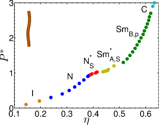
Figure 5: Equation of state for helices having $r=0.2$ and $p=8$. Different colours indicate different phases: I=isotropic; N=nematic; N${}_{S}^{*}$=screw-nematic; Sm${}_{A,S}^{*}$=screw-smectic A; Sm_B,p= smectic B polar.

Different phases can be distinguished with the help of the order parameters and correlation functions defined in Section II.3. At low $\eta$ the system is in the I phase, but, as $\eta$ approaches a value $\approx 0.23$, helices tend to align their long axis ($\widehat{\mathbf{u}}$) along a common direction, the main director $\widehat{\mathbf{n}}$. The onset of the nematic phase is signaled by a jump of the order parameter $\langle P_{2}\rangle$ to a value $\sim 0.4$, as shown in Fig.6 (left panel). This is the conventional N phase, as indicated by the absence of translational order and the low or vanishing value of all the other order parameters defined in section II.3. Above $\eta\approx 0.4$, Fig.6 (right panel) illustrates how the $\langle P_{1,c}\rangle$ order parameter has a marked upswing, the signature of screw-like ordering: the C₂ axes of helices ($\widehat{\mathbf{w}}$) tend to preferentially align along a common axis $\widehat{\mathbf{c}}$, orthogonal to $\widehat{\mathbf{n}}$ and spiralling around it. Unlike the nematic, this order is locally polar, i.e. the $\widehat{\mathbf{w}}$ vectors on a given plane perpendicular to $\widehat{\mathbf{n}}$ preferentially point to the same direction.

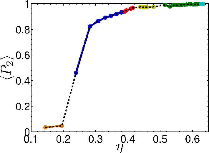
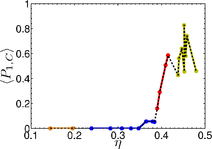
Figure 6: Order parameters $\langle P_{2}\rangle$ and $\langle P_{1,c}\rangle$, for helices with $r=0.2$ and $p=8$. Different colours indicate state points belonging to different phases (see fig. 5).

Additional insights on the onset of the N${}_{S}^{*}$ phase are provided by the correlation functions $g_{\|}(R_{\|})$ and $g_{1,\|}^{\widehat{\mathbf{w}}}(R_{\|})$, shown in Fig. 7,

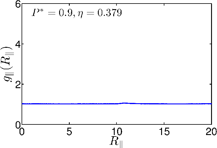
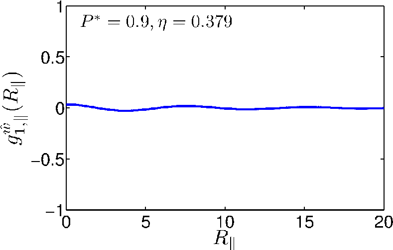
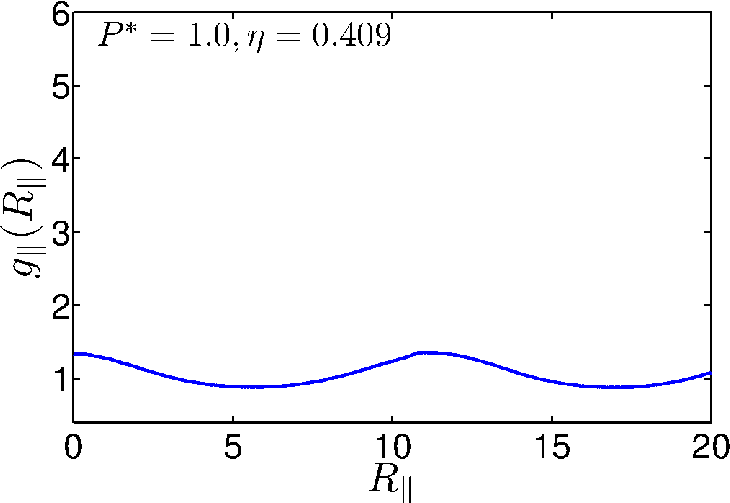
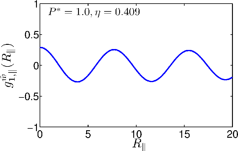
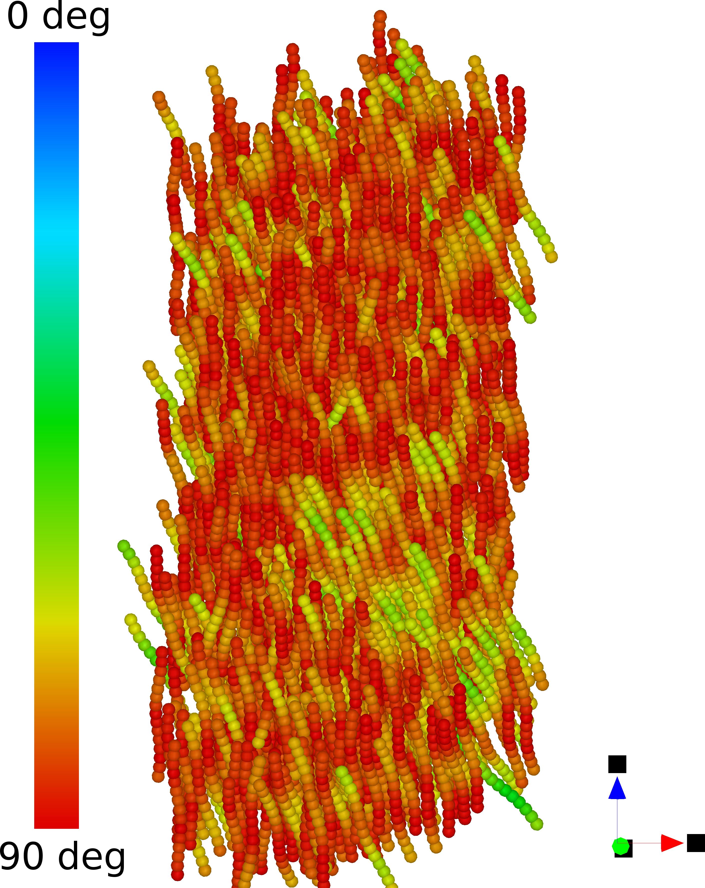
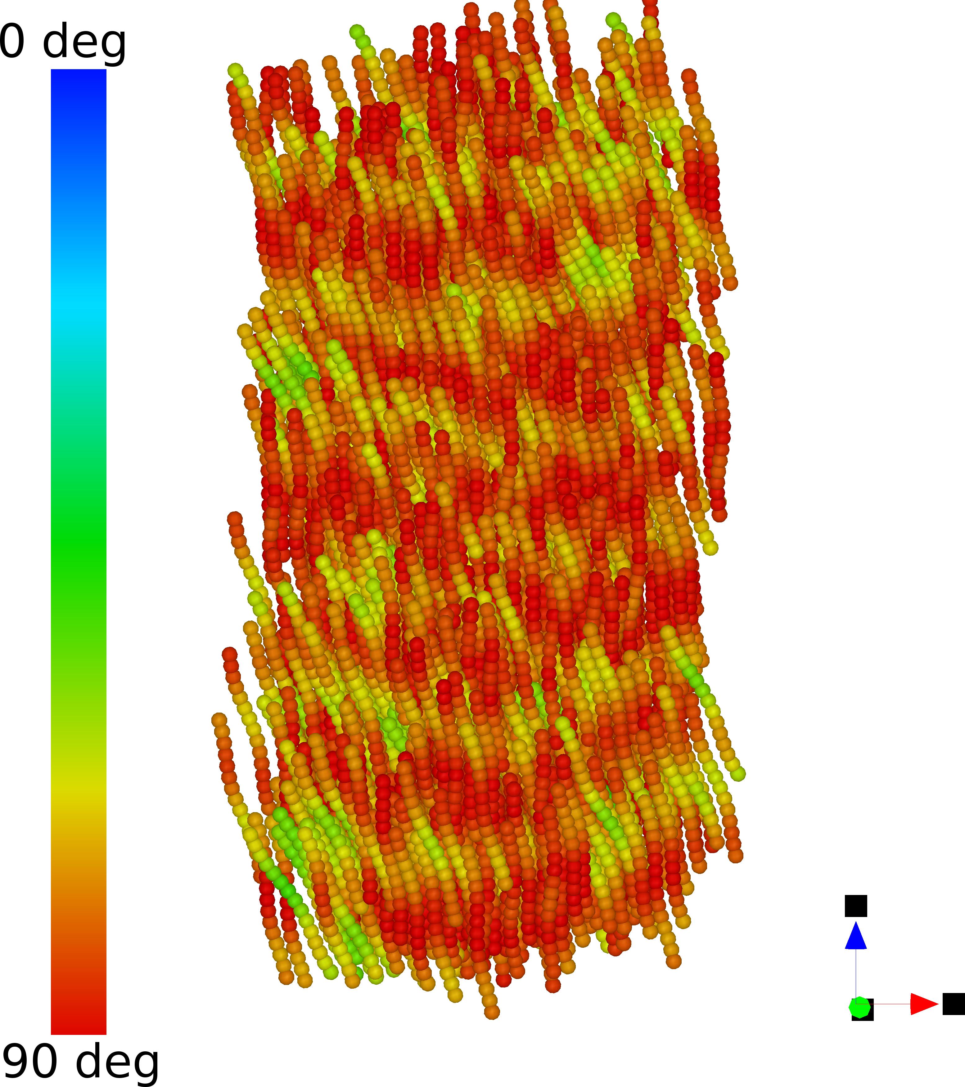
Figure 7: The $g_{\|}(R_{\|})$ and $g_{1,\|}^{\widehat{\mathbf{w}}}(R_{\|})$ correlation functions for helices with $r=0.2$ and $p=8$, calculated for $P^{*}=0.9$ in the $N$ phase (left) and $P^{*}=1.0$ in the N${}_{S}^{*}$ phase (right). Also depicted are two corresponding snapshots, colour coded according to the local tangent as explained in the text.

for two selected state points corresponding to pressure $P^{*}=0.9$ and $P^{*}=1.0$, across the N–N${}_{S}^{*}$ phase transition. One can clearly notice the difference in the behaviour of $g_{1,\|}^{\widehat{\mathbf{w}}}(R_{\|})$ at the two sides of the phase transition, with the function at $P^{*}=1.0$ showing a well developed periodicity that matches the pitch of helices $p$. The sinusoidal behaviour of $g_{1,\|}^{\widehat{\mathbf{w}}}(R_{\|})$ is representative of an azimuthal correlation in planes perpendicular to $\widehat{\mathbf{n}}$, indeed a footprint of the N${}_{S}^{*}$ phase. A glance at two snapshots Gabriel08 also reported in Fig. 7 gives a visual support of this interpretation. Here, as well as in other snapshots reported henceforth, helices are colour coded according to their $P_{2}(\cos\theta)$ value, where $P_{2}$ is the second Legendre polynomial and $\theta$ is the angle between the local tangent to helices and an arbitrarily chosen axis, not parallel to the main director ${\widehat{\mathbf{n}}}$. This angle changes as the tangent moves along a helix, so that $P_{2}(\cos\theta)$ and then the colour changes, with a periodicity equal to half the pitch $p$. Therefore, the regular stripes occurring in the bottom right snapshot of Fig. 7 corresponding to the N${}_{S}^{*}$ state point ($P^{*}=1$), but absent in the bottom left snapshot corresponding to the N state point ($P^{*}=0.9$), highlight the different organization occurring at the two pressures.

In Fig. 7 one can further notice a small amplitude oscillation in function $g_{\|}(R_{\|})$ at $P^{*}=1$, that is absent in the corresponding lower pressure case $P^{*}=0.9$. This is indicative of an incipient smectic order, which sets in at the slightly higher pressure $P^{*}=1.1$, as confirmed by the solid-like behaviour of $g_{\|}(R_{\|})$ shown in Fig.8 (top left). Here we can recognize a periodicity of $\sim 12$, only slightly longer than the effective length of the helices, which is equal to 10.88. This is different from the periodicity of $g_{1,\|}^{\widehat{\mathbf{w}}}(R_{\|})$ (top right), which corresponds to the helix pitch $p$, here equal to 8. Thus the screw-like order has combined with layer ordering to give rise to a new chiral smectic phase. The presence of two different periodicities is evident in the snapshot in Fig. 8. The correlation function $g_{\perp}(R_{\perp})$ (Fig. 8, bottom left) does not provide indication of translational order within each single layer, and $\langle\psi_{6}\rangle$ is found to be very small. This screw-smectic phase, globally uniaxial with the main director perpendicular to the layers, is of type $A$ and labelled as Sm${}_{A,S}^{*}$.

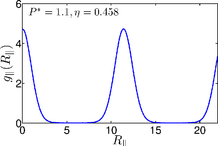
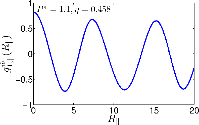
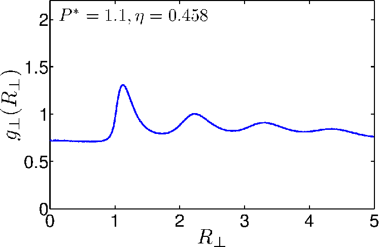
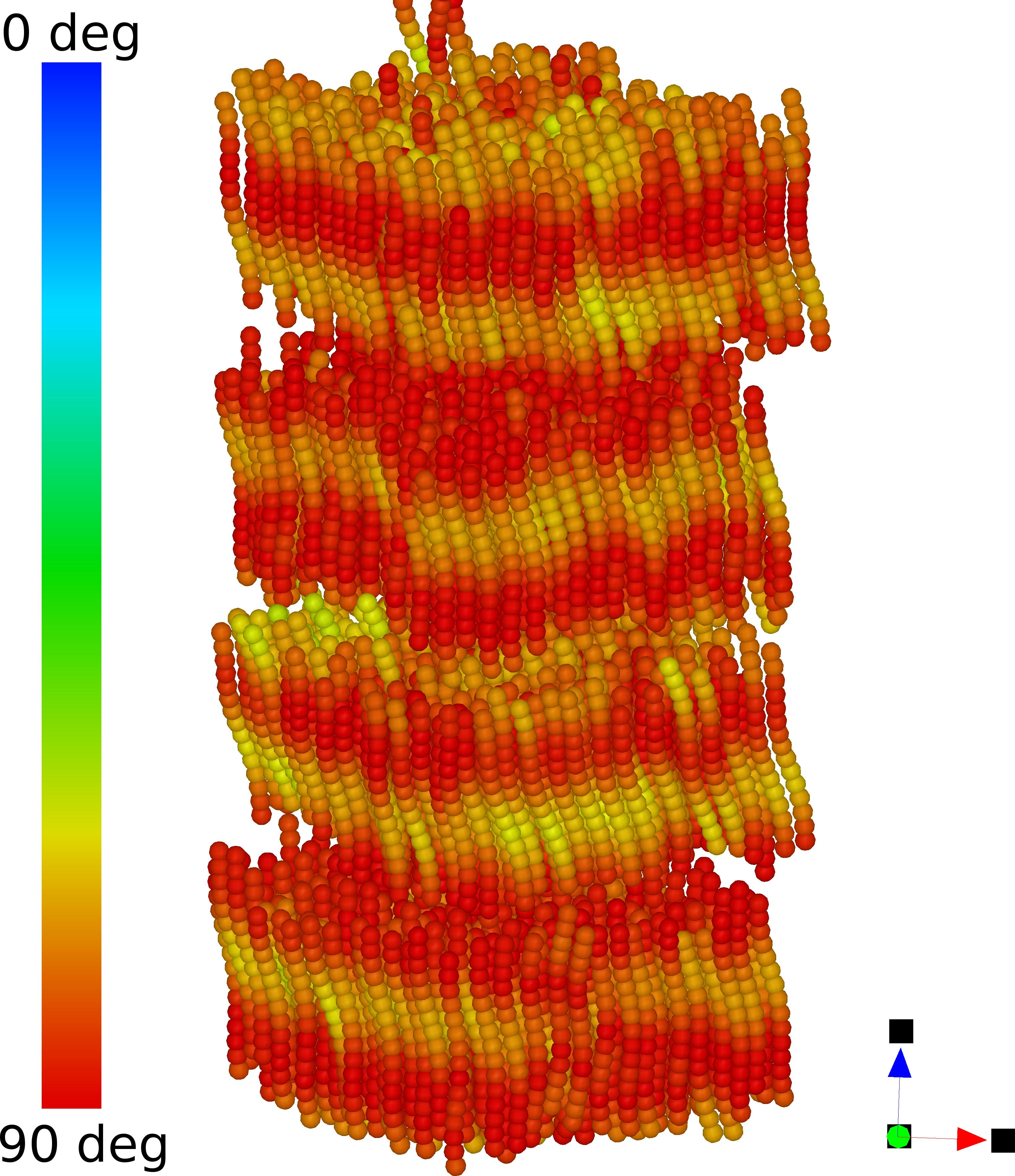
Figure 8: The functions $g_{\|}(R_{\|})$ (top left) and $g_{1,\|}^{\widehat{\mathbf{w}}}(R_{\|})$ (top right) at $P^{*}=1.1$, for helices with $r=0.2$ and $p=8$ (Sm${}_{A,S}^{*}$ phase.. Also depicted is $g_{\perp}(R_{\perp})$ and a corresponding snapshot colour coded according to the local tangent to helices (right).

At higher pressure, $P^{*}=1.3$ ($\eta\approx 0.52$), hexatic order sets in within each single layer, as shown by the behavior of $g_{\perp}(R_{\perp})$ that exhibits well developed characteristic double peak structure, with maxima at $\sqrt{3}\sigma$ and $2\sigma$ (Fig. 9, left panel), $\sigma$ being the position of the main, nearest-neighbour peak. The presence of hexatic order is further confirmed by the high value of $\langle\psi_{6}\rangle$ (Fig.10 left panel) and by the fact that the average number of nearest-neighbours $\langle n\rangle$ tends to $6$ at $\eta\approx 0.52$. The plot of $g_{1,\|}^{\widehat{\mathbf{w}}}(R_{\|})$ (Fig.9, top right panel) shows a clear in-plane azimuthal correlation, but the absence of the helical periodicity that was present in the Sm${}_{A,S}^{*}$ phase. The correlation now is only within layers, which are uncorrelated from each other. This difference from the Sm${}_{A,S}^{*}$ phase clearly appears from comparison of the relative snapshots of Fig. 8 with those of Fig. 9. We refer to this phase as smectic B polar (Sm_B,p), to highlight the presence of hexatic order combined with polarity within layers. Note that the gaps appearing in the $g_{1,\|}^{\widehat{\mathbf{w}}}(R_{\|})$ are indicative of the absence of particles with those particular $R_{\|}$ values and are specific of state points at very high density.

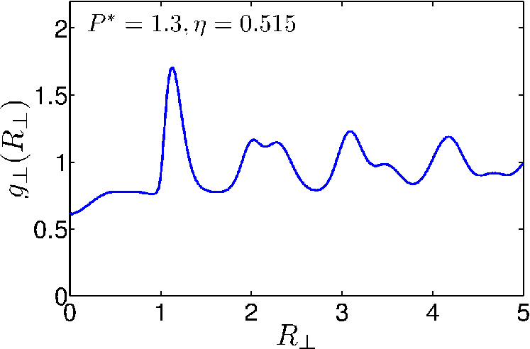
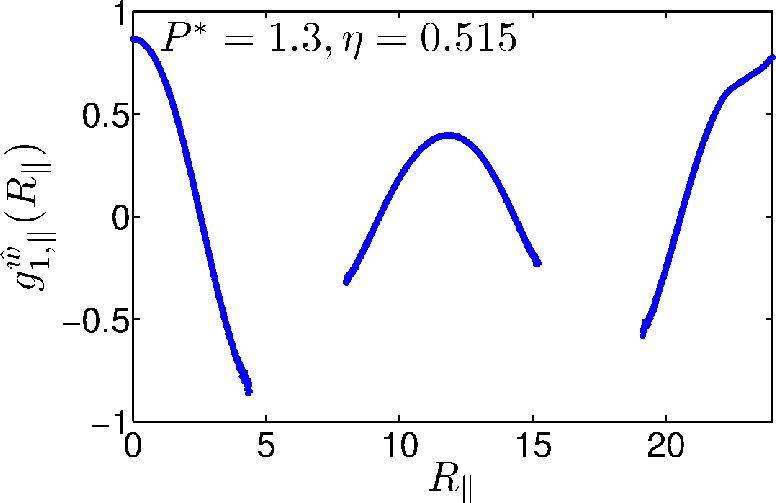
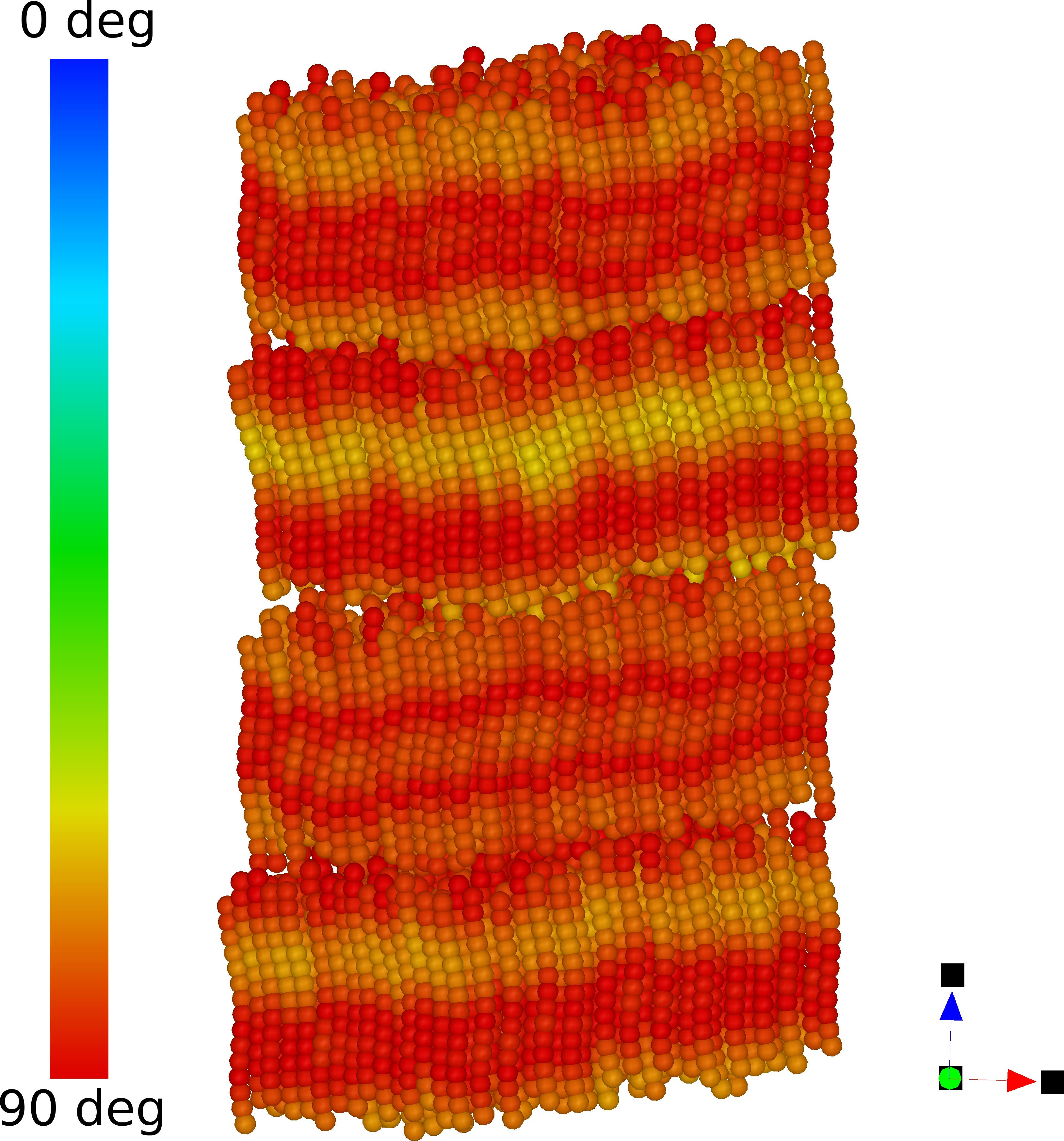
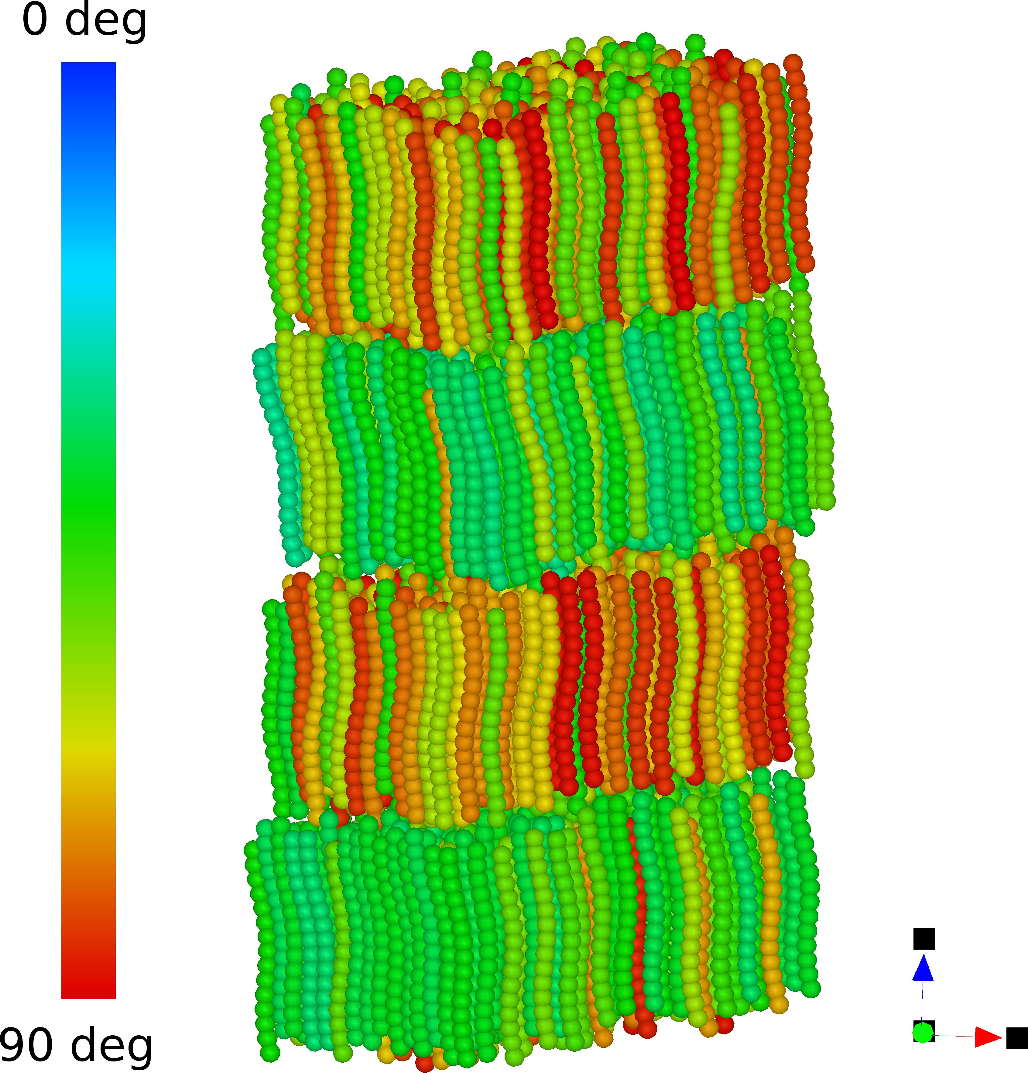
Figure 9: Behaviour of $g_{\perp}(R_{\perp})$ (left) and $g_{\|}(R_{\|})$ (right) and relative snapshot, colour coded according to the local tangent (left) and to the C₂ axis (right) at $P^{*}=1.3$, in the case $r=0.2$ and $p=8$. This state point belongs to the Sm_B,p phase. Note that in the case of the C₂ axis, azimuthal rotations of angles in the range $[90^{\circ},180^{\circ}]$ are colour coded in the same way as in the case $[0^{\circ},90^{\circ}]$ because of the limitations in the QMGA software Gabriel08 . For this reason, this color coding will not be further exploited in the remaining of the paper.

Figure 10: Hexatic order parameter $\langle\psi_{6}\rangle$ and average nearest-neigbour number $\langle n\rangle$, both indicative of in-plane hexatic ordering, for helices with $r=0.2$ and $p=8$. State points belonging to different phases are colour as in Fig. 5.

On increasing the helical twist, the onset of unconventional screw-like phases becomes more and more pronounced. We first keep the radius fixed at $r=0.2$ and decrease the pitch down to $p=4$. The equation of state and corresponding order parameters are reported in Fig.11. As for the case $r=0.2$ and $p=8$, there are both the N and the N${}_{S}^{*}$ phase, but the latter becomes predominant in this case. Also the higher density smectic phase exhibits new features, with the $\langle P_{1,c}\rangle$ order parameter being large throughout the entire smectic range and a final sudden drop only at the onset of the compact phase C. Thus all smectic phases exhibit screw-like order. However they are distinguished by the profile of $g_{\perp}(R_{\perp})$ and by a substantially different behaviour of $\langle\psi_{6}\rangle$, which is larger in the state points belonging to the phase denoted as Sm${}_{B,S}^{*}$ than the Sm${}_{A,S}^{*}$ phase. Perhaps surprisingly, the average nearest-neighbour number $\langle n\rangle$ in the Sm${}_{B,S}^{*}$ phase remains significantly smaller than $6$, in spite of the large value of $\langle\psi_{6}\rangle$. As remarked, this quantity is very sensitive to the definition of the nearest-neighbour distance that contains a significant degree of arbitrariness, and hence might be more accurate for some state points than others. A top view of the relative snapshots none the less confirms the presence of a hexatic ordering in the state points labelled as Sm${}_{B,S}^{*}$ and not in those labelled as Sm${}_{A,S}^{*}$.

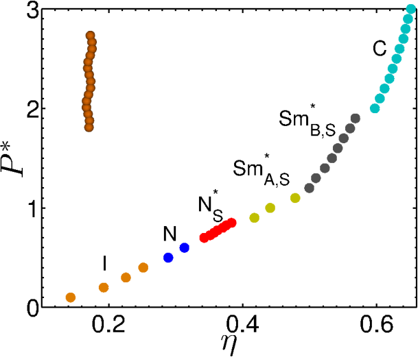
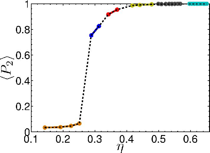
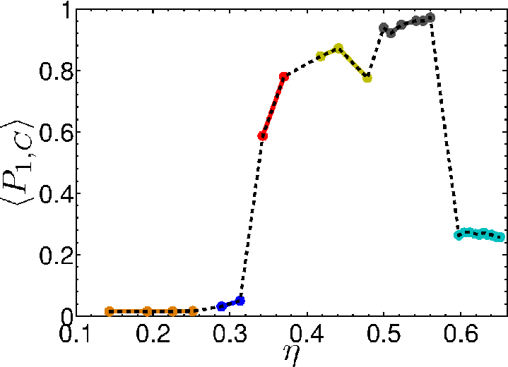
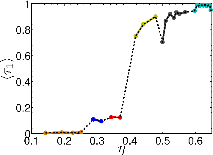
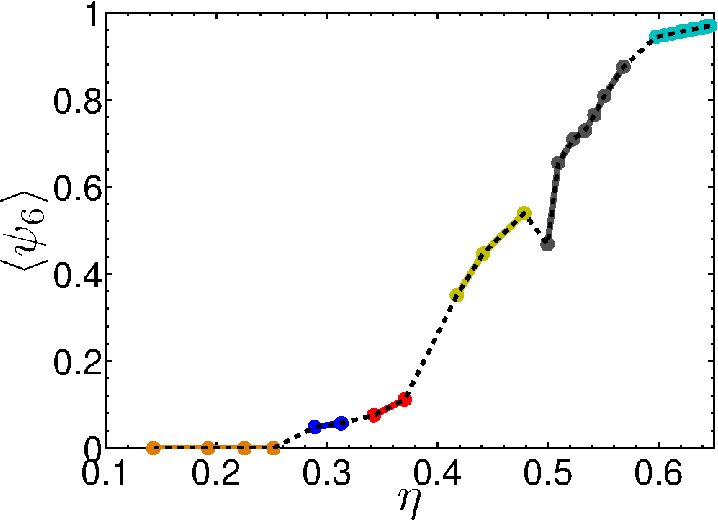
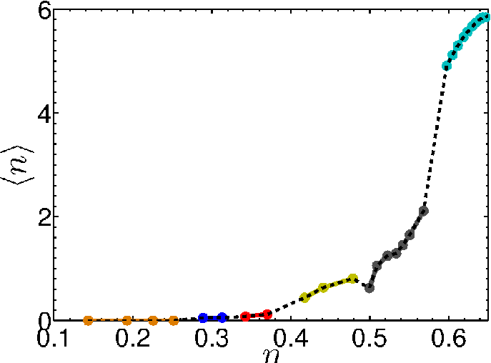
Figure 11: Equation of state and order parameters $\langle P_{2}\rangle$, $\langle P_{1,c}\rangle$, $\langle\tau_{1}\rangle$, $\langle\psi_{6}\rangle$ and average nearest-neigbors $\langle n\rangle$, (in typewriter order) in the case $r=0.2$ and $p=4$. Note that in the plot for the equation of state (top,left), additional points between the two extrema, have been included in the N${}_{s}^{*}$ phase, for completness.

The ”curliest” among the investigated helices are those with $r=0.4$ and $p=4$, whose morphology is displayed in the inset of Figure 12 showing the equation of state.

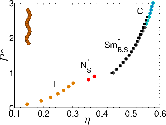
Figure 12: Equation of state for helices with $r=0.4$ and $p=4$. Filled circles refer to the same initial conditions used throughout this work, whereas filled darker squares refer to different initial condition, as detailed in the text.

This exhibits important differences with the phase diagram reported in Figs. 5 and 11, with only two intermediate high-density liquid crystal phases being present, the N${}_{S}^{*}$ and Sm${}_{B,S}^{*}$. The system then undergoes a direct first-order transition from the I to the N${}_{S}^{*}$ phase, without an intermediate N phase. This behaviour can be ascribed to the combined effect of significant twist and small effective aspect ratio, in agreement with the interpretation given above of the results obtained for the less curly helices. One more novel feature is a direct transition from the N${}_{S}^{*}$ phase to a smectic phase with in-plane ordering Sm${}_{B,S}^{*}$. The profile of $g_{\|}(R_{\|})$ obtained at $P^{*}=1.5$ (Fig. 13 top panel) indicates layering with a periodicity close to the effective helix length, 9.47 in the present case. Hexatic in-plane order is inferred from the behavior of $g_{\perp}(R_{\perp})$ (Fig. 13 central panel) and from the corresponding high value of $\langle\psi_{6}\rangle$. However, differently from Sm_B,p phase (Fig. 9), here there is additional screw-like ordering, with a period equal to the helix pitch $p=4$, which is evidenced by the correlation function $g_{1,\|}^{\widehat{\mathbf{w}}}(R_{\|})$ (Fig. 13 bottom panel) and by the high $\langle P_{1,c}\rangle$ order parameter. Another interesting feature supporting the Sm${}_{B,S}^{*}$ nature of the smectic phase is included in the (red) dotted line of $g_{\perp}(R_{\perp})$ (Fig. 13 central panel) that reports the behaviour of $g_{\perp}(R_{\perp})$ when the average is limited to a single layer. In particular, the absence of the first peak at $R_{\perp}\approx 0$ in this case, and conversely present when the average is carried out over all layers, is a clear indication of a AAA structure, reminiscent of a columnar structure, where a helix belonging to a given layer locks with the one stacked immediately on its top, and belonging to the successive layer, to form an essentially ”infinite” helix spanning the full computational box.

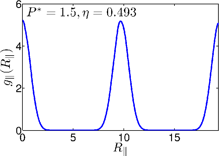
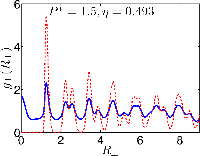
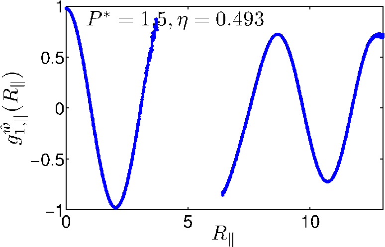
Figure 13: Top left panel. Plot of $g_{\|}(R_{\|})$ in the case of $r=0.4$, $=4$, at reduced pressure $P^{*}=1.5$ (Sm${}^{\ast}_{B,S}$ phase). Top right panel. Profile of $g_{\perp}(R_{\perp})$ calculated by averaging over all layers (solid line) and over a single layer (red dotted line). Bottom panel. Behavior of $g_{1,\|}^{\widehat{\mathbf{w}}}(R_{\|})$.

This essential difference between the structure of the Sm${}_{B,S}^{*}$ and the Sm${}_{B,p}^{*}$ phases is summarized in the sketch of Fig. 14. While in the Sm${}_{B,S}^{*}$ phase (Fig. 14 left) helices are azimuthally correlated within each plane and screw-like correlated between different planes, in the Sm_B,p phase (Fig. 14 right) only intra-plane azimuthal correlation is present, with different layers being uncorrelated both positionally and orientationally.

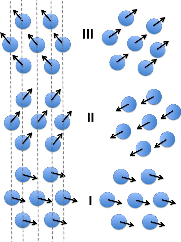
Figure 14: Cartoon of the smectic B phases discussed in the text. Circles represent transversal sections through the center of helices and arrows the corresponding $\widehat{\mathbf{w}}$ vectors. I,II, III indicate adjacent layers. Left: Sm${}_{B,S}^{*}$ phase, with through-layers positional correlation (AAA structure, highlighted by the dashed lines) and screw-like (orientational) correlation of $\widehat{\mathbf{w}}$ vectors. Right: Sm_B,p phase, with in-layer correlation of $\widehat{\mathbf{w}}$ vectors and neither positional nor orientational correlation between layers.

Given the crucial role that starting configurations may have at high density, as a final point it is instructive to dwell on their effect on the final phase diagram. We remind at this stage that all results discussed so far were obtained by starting from a very compact initial configuration, obtained by the ISM and then equilibrated at the appropriate value of $P^{*}$. While for the isotropic and nematic phases a different initial condition would result into an almost indistinguishable picture, this is not necessarily true for higher density phases, as it also happens in the case of hard spherocylinders.Bolhuis97 This turns out to be also the case here, as reported in Fig.12, where the original results (filled circles) are contrasted with those obtained starting from an equilibrated configuration at the immediately lower pressure (filled squares). In both cases the first smectic point was obtained from the original compact configuration. This small reagion of hysteresis indicates a maximal range of uncertainty of the true thermodynamic coexistence pressure. The results collected so far point to the existence of a first-order transition between the Compact and the Smectic phases: the hysteresis observed may be interpreted as a signal of it.

III.2 Locating the isotropic-to-nematic phase transition

It proves of interest, at this stage, to discuss how to properly locate the volume fractions and pressure at the isotropic–nematic coexistence. The most direct method is a technique known as Successive Umbrella Sampling (SUS),Virnau04 originally developed for the calculation of the gas-liquid coexistence in the grand-canonical ensemble. In the isotropic-nematic coexistence of hard rods this has been discussed in Ref.Vink05 . Although it could be clearly applied to the present case as well, we have found this to be particularly problematic as a result of the combination of the sole hard-core interactions and of the reduced aspect ratio. As the aspect ratio decreases, the I–N transition shifts to higher densities, and insertion of a particle becomes increasingly harder. This agrees with a similar observation made by the authors of Ref.Vink05 , who estimated $15$ as the minimum aspect ratio to study the phase transition with a reasonable computational effort, whereas our helices have typical aspect ratios of the order of $10$ or less. This notwithstanding, SUS can still be applied to a helical particle system by using a somewhat more elaborate procedure that will be discussed elsewhere.

Under these conditions, we have here found it more convenient to resort to a different procedure that, albeit less direct, is still able to provide a rather accurate value of the coexisting densities and pressure. The basic idea is to perform, via MC-NVT simulations, a detailed description of the equation of state across the I–N transition, and then use an equal area construction to infer the coexisting volume fractions and pressure. This is depicted in Fig. 15 in the case $r=0.2$ and $p=4$, which is a blow-up of the case analyzed in Fig.11 close to the I–N phase transition. The Mayer-Wood loop Mayer65 is consistent with a first order transition, and an equal area construction provides the two coexisting volume fractions $\eta_{I}=0.2642\pm 0.0002$ and $\eta_{N}=0.2772\pm 0.0001$ (crossed points) at pressure $P_{IN}=0.4805\pm 0.0035$ (dotted line). Notwithstanding the finite size effects, it is worth noticing that the precision and reliability of this result does not unfavourably compare with those usually obtained via SUS calculations.

These findings can be contrasted with those obtained via the DFT theory, eq. 20, as illustrated in Section II.4. This result is also reported in Fig.15 as a thick solid line. Roughly speaking, we find DFT to underestimate the coexistence pressure by $\approx 15\%$ and the coexistence densities by $\approx 4\%$. This is consistent with previous comparison with NPT simulations Frezza13 and with the typical accuracy achieved by DFT calculations.

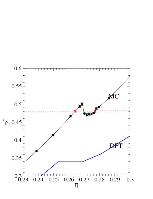
Figure 15: Equal area construction in the case of $r=0.2$ and $p=4$. Points are results from MC simulations, traversed by their Akima spline interpolation. Resulting values for coexisting volume fractions are $\eta_{I}=0.2642\pm 0.0002$ and $\eta_{N}=0.2772\pm 0.0001$ (crossed points) at pressure $P_{IN}=0.4805\pm 0.0035$ (dotted line). Also displayed are the results from DFT (think solid line).

III.3 Theoretical description of the nematic–screw-nematic phase transition

In this Subsection, we will assess the accuracy of the various DFT approximations introduced in Section II.4 to investigate the N-N${}_{S}^{*}$ transition, through a direct comparison with numerical simulations. To this aim, we will consider the particular case of helices having full translational and azimuthal freedom, but with their $\hat{\mathbf{u}}$ axis parallel to the $\hat{\mathbf{n}}$ director. This assumption, partly justified by the observation that the N-N${}^{*}_{S}$ phase transition occurs at large values of the nematic order parameter, has the advantage of simplifying the theoretical treatment and considerably reducing its computational cost. This notwithstanding, it can still be useful for several different reasons. Firstly, it provides direct insights into the order of the N-N${}_{S}^{*}$ transition, and its relationship with the helix morphology, decoupled from the effects of the particle structure on the stability of the nematic phase. Secondly, it allows us to probe the reliability of theory to describe this rich and unconventional scenario. Finally, it is an interesting problem on its own right as the behavior of non-convex hard particles has so far largely overlooked in spite of the large number of examples in real systems.

We remark that, unlike previous cases, we have here used the number of complete turns ($n$) as input variable, thus resulting in a non-integer pitch value $p$. The relation between $n$ and $p$ can be found in Ref.Frezza13 . Fig. 16 gives an example of the function $a_{excl}(\zeta^{\prime},\gamma^{\prime})$ (Eq. 21), for the case with $r=0.4$ and $p=4.322$. This function exhibits oscillations, whose number reflects the number of turns in the helix. Oscillations are comprised between the values of excluded area for cylinders enclosing the whole helix ($a_{excl}=\pi(2r+1)^{2}$) and for cylinders enclosing a linear chain of beads ($a_{excl}=\pi$), as they should. The decrease of $a_{excl}$ resulting from the interpenetration of helices is related to the entropy gain that drives the formation of the N${}_{S}^{*}$ phase.

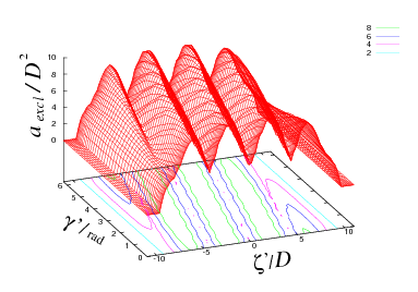
Figure 16: The function $a_{excl}(\zeta^{\prime},\gamma^{\prime})$ (see Eq. 21), calculated for helices with $r=0.4$ and $p=4.322$.

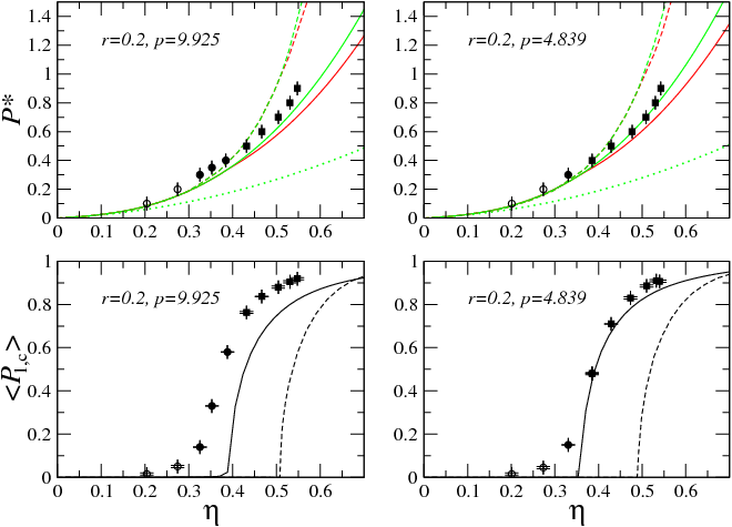
Figure 17: Equation of state (top) and screw-nematic order parameter as a function of the volume fraction $\eta$ (bottom), for perfectly aligned hard helices with $r=0.2$ and $p=9.925$ (left) and $p=4.839$ (right). Results from Onsager theory (dotted), from modified PL theory (dashed) and from third-virial theory (solid). Top panels: green is for the N phase and red for the N${}_{S}^{*}$ phase. Symbols are results from MC simulations: N (empty circles), N${}^{*}_{S}$ (full circles) and Sm${}_{S}^{*}$ (full squares).

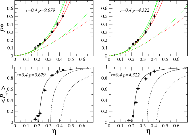
Figure 18: Equation of state (top) and screw-nematic order parameter as a function of the volume fraction $\eta$ (bottom), for perfectly aligned hard helices with $r=0.4$ and $p=9.679$ (left) and $p=4.322$ (right). Results from Onsager theory (dotted), from modified PL theory (dashed) and from third-virial theory (solid). Top panels: green is for the N phase and red for the N${}_{S}^{*}$ phase. Symbols are results from MC simulations: N (empty circles), N${}^{*}_{S}$ (full circles) and Sm${}_{S}^{*}$ (full squares).

Fig. 17 shows equation of state and screw-nematic order parameter as a function of $\eta$ for the cases with $r=0.2$ and $p=9.925$ and $4.839$, while Fig. 18 shows the same quantities for the cases with $r=0.4$ and $p=9.679$ and $4.322$. These figures provide results from second- and third-virial theories along with corresponding MC simulation data. We can see that for these helices, which have a pitch larger than the bead diameter, the location of the phase transition is essentially determined by the radius $r$, depending mildly on $p$, and in particular it occurs at increasing density with decreasing radius. This can be understood considering that less curly helices have weaker oscillations of $a_{excl}$, thus a lower entropy gain is achieved for them upon the settling in of the screw-like order. Present results would seem to hardly reconcile with the phase diagrams shown in Sec. III A, where the N-N${}^{*}_{S}$ phase transition occurs at a volume fraction that increases on moving from $r=0.2$, $p=4$, to $r=0.4$, $p=4$ and then to $r=0.2$, $p=8$. However, it has to be recalled that, on one hand, the hard helices considered here have the same contour length and their effective aspect ratio thus decreases on going from straight to curly particles and, on the other hand, that in the MC-NPT simulations helices are freely rotating. The onset of any liquid-crystalline order thus always competes with the I phase, favoured at low densities and whose stability shifts to higher densities as the effective aspect ratio becomes smaller.

Compared to MC data for perfectly aligned helices, while a purely second-virial theory alone proves overall inadequate, significant improvements are achieved including PL correction and the third-virial term. By looking at each and confronting one another all these figures, it seems that the predictions of a third-virial theory improve as $r$ increases and $p$ decreases, to such an extent that, for the cases with $r$=0.4 quantitative agreement is there between theory and simulations. This situation is in a way spoilt by the fact that the phase observed in simulations at higher densities is actually a Sm${}_{S}^{*}$ note6 rather than a N${}_{S}^{*}$ phase. Theoretical calculations that include the former are not available at present (it would amount to deal with Eq.15 rather than simpler Eq.16). In spite of this caveat, results from a third-virial theory are considered overall encouraging.

IV Discussion

We are now in the position to try and understand the physical origin of the phase sequence exhibited by helical particles. The nematic phase spans a density range that can be subdivided in two regions, the first being the conventional N phase at lower densities, the second being the screw-like N${}_{S}^{*}$ phase at higher density. The relative width of the two regions varies depending upon the helix parameters, but with the screw-like N${}_{S}^{*}$ phase always popping out at the right edge of the nematic window, while the N phase may or may not be present. Indeed, the latter can be absent altogether for sufficiently high degree of curliness as shown by our results in the case of $r=0.4$ and $p=4$. Indeed, on increasing the helical twist, the relative width of the screw-like region increases with respect to the conventional N region, until the latter eventually disappears. The underlying mechanism is as follows.

Imagine to have two neighbouring helices that are sufficiently far apart to be able to rotate about their own main axis. Effectively, they behave as cylinders, their specific helix character being rather irrelevant and the liquid-crystal phase they may be in is the conventional N phase. This is however no longer the case if the two helices are in close contact one another so that neighbouring grooves significantly intrude into each other into a in-phase locked configuration, as illustrated in Fig.19. Because of this azimuthal locking of the C₂ axes, there is then a severe limitation of the rotational entropy and there must then be a correspondingly higher gain in translational entropy in order for the new chiral nematic phase to be stable with respect to the N phase. This is achieved through a screw-like organization, schematically illustrated in Fig.19 where the right helix rotates about its own axis by performing an additional translation along the same axis.

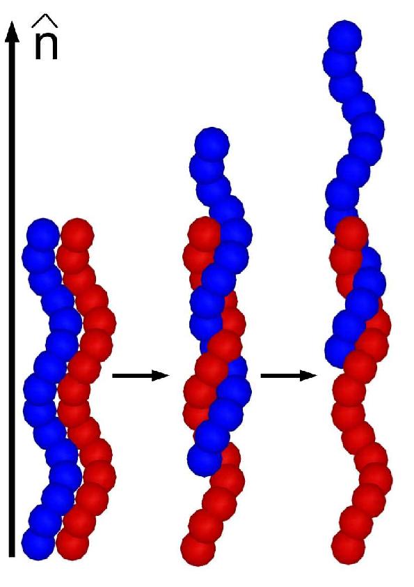
Figure 19: The screw-like coupled translation and rotation.

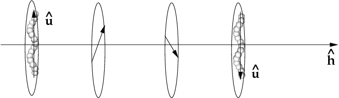
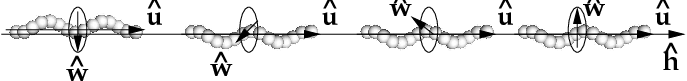
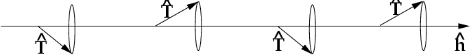
Figure 20: Cartoon of the cholesteric (top), and of the screw-nematic (middle) organization. Here $\widehat{\mathbf{h}}$ is a unit vector parallel to the axis around which either the molecular axis $\widehat{\mathbf{u}}$ (cholesteric) or $\widehat{\mathbf{w}}$ (screw-nematic) spirals, respectively. In the latter case, the tip of the tangent to the helices $\widehat{\mathbf{T}}$ forms a conical path (bottom).

The N${}_{S}^{*}$ is a novel kind of chiral nematic phase, different from the well known cholesteric. The latter may be formed in general by any kind of chiral mesogenic particles, whereas the former is special of helical particles. It may be useful to highlight analogies and differences between these phases. In the cholesteric phase the $\widehat{\mathbf{u}}$ axes of helices spiral around a perpendicular axis ($\widehat{\mathbf{h}}$) as illustrated in Fig.20 (top). The order of the $\widehat{\mathbf{u}}$ axes is non-polar, i.e. there is up-down symmetry. In the N${}_{S}^{*}$ phase the $\widehat{\mathbf{u}}$ axes of helices are preferentially aligned along the same direction throughout the sample, but the transversal $\widehat{\mathbf{w}}$ axes spiral around this direction, as depicted in Fig. 20 (center). In this case the $\widehat{\mathbf{w}}$ axes have polar order, i.e. they preferentially point in the same direction. Another important difference between screw-nematic and cholesteric is the length scale of the phase periodicity, which is equal to the pitch of the helical particles in the former, and orders of magnitude longer in the latter. This is the reason why the screw-like organization, unlike the cholesteric, can be observed in simulations with box sizes of a few molecular lengths and standard periodic boundary conditions.

A different description of the screw-nematic phase could be made, in terms of the Frenet frame routinely used for the description of flexible and semi-flexible polymers (e.g. Kamien02 ). This however provides a redundant description for rigid objects of finite lengths as the helices considered in the present work. Using this picture, the tip of the local tangent the helices ( $\widehat{\mathbf{T}}$) follows a conical path on moving along the director $\widehat{\mathbf{n}}$, due to the variation of the azimuthal angle at fixed polar angle, as shown in Fig.20 (bottom). This was the description used in Ref.Barry06 to explain the experimental results for helical flagella and that led to denoting this phase as conical.Meyer68 ; Kamien96 We also have found it useful for the visualization of snapshots colour coded according to the local tangent of helices.

The situation is expectedly much more complex in smectic phases, where screw-like organization, layering and hexatic order may compete and combine one another. As the system is entering a smectic phase, there still exists a non-negligible fraction of interlayer helices while positional ordering along the $\widehat{\mathbf{n}}$ direction progressively increases. These helices lying in the interlayer regions provide a bridge between two adjacent layers, and allow a screw-like organization to be present througout the whole smectic phase. When the concentration of helices is still moderate, hexatic ordering is not significantly present and the first smectic phase encountered upon increasing density is the Sm${}_{A,S}^{*}$. As in the nematic phase, this roto-translational coupling may be more or less effective depending upon the morphology of the helix, but is always present in the initial part of the smectic phases.

As pressure is further increased, the hexatic order gradually sets in, typically accompanied by a concomitant increase of the azimuthal correlation of the $\widehat{\mathbf{w}}$ axes of helices within each layer. This may lead to two different, and up to a certain extent competing, effects. The first possibility is that helices are azimuthally aligned within each each layer, but with neither positional nor orientational correlations between layers. Each layer can also in principle rigidly slide with respect to next layers, to gain translational entropy. Under these conditions, layering is very strong as testified by the solid-like peaks in the observed $g_{\|}(R_{\|})$. This situation, depicted in the cartoon of Fig.14 (right panel), differs from the conventional smectic B phase for the presence of the in-plane (polar) correlation between the $\widehat{\mathbf{w}}$ axes of helices, and hence the phase was denoted as Sm_B,p.

The alternative scenario stems from the possibility that tips of helices protruding out from a layer are still able to propagate the ordering to the neighboring layers. Thus, helices belonging to different layers stack on top of each other along $\widehat{\mathbf{n}}$ to form parallel, ”infinitely” long, helices. The alignement of the the $\widehat{\mathbf{w}}$ axes then translates into a screw-like ordering propagating across the layers. Under these conditions, clearly different layers are strongly correlated with each other. The layer structure along $\widehat{\mathbf{n}}$ is preserved, but positional ordering along $\widehat{\mathbf{n}}$ is less effective, due to the presence of protruding helices, as testified by the reduced peaked structure of $g_{\|}(R_{\|})$. This is the situation represented in the left panel of Fig.14. We denoted this phase as Sm${}_{B,S}^{*}$, because it couples layering with hexatic positional order and screw-like azimuthal correlations. The entropic advantage of this scheme is to form a set of ”infinite” parallel helices, which allows the favourable screw-like motion to be still operative. One may envisage the additional presence of a columnar phase in the case of helices with sufficiently long contour lengths, well beyond those considered here. This is a subject that deserves a dedicated study.

V Conclusions and outlook

Phase	Code	Organisation type
Conventional nematic	N	$(a)$
Screw- nematic	N${}_{S}^{*}$	$(b)$
Screw-smectic A	Sm${}_{A,S}^{*}$	$(c)$
Polar smectic B	SmB,p	$(d)$
Screw-smectic B	Sm${}_{B,S}^{*}$	$(e)$

Table 1: Summary of the different phases exhibited by hard helices. $(a)$$\widehat{\mathbf{u}}$ axes oriented along $\widehat{\mathbf{n}}$; $(b)$ as in N with azimuthal coupling of $\widehat{\mathbf{w}}$ axes along $\widehat{\mathbf{c}}$ that in turn spirals about $\widehat{\mathbf{n}}$; $(c)$as in Sm_A with azimuthal coupling of $\widehat{\mathbf{w}}$ axes along $\widehat{\mathbf{c}}$ that in turn spirals about $\widehat{\mathbf{n}}$; $(d)$ as in Sm_A with additional in-plane polar and hexatic order; $(e)$ as in Sm${}_{A,S}^{*}$ with additional hexatic order.

In this work, we have studied the self-assembly properties of systems of hard helices as a function of helix morphology. Helical particles have been modelled as a set of fused hard spheres properly arranged to form a rigid helix of a fixed contour length. Using a combination of numerical simulations and density functional theories, we have analyzed the sequence of different liquid crystal phases appearing at increasing density, using a set of suitable order parameters and correlation functions.

The rich and unconventional polymorphism that we found is in striking contrast with the conventional wisdom of assimilating the phase behaviour of helical particles to that of rods, an assumption commonly adopted also in the analysis of experiments on helical (bio)polymers. Table 1 summarizes the distinctive features of all phases discussed in this work.

The first novel phase encountered with increasing density is the screw-nematic (N${}_{S}^{*}$). As neighboring helices tend to lock into an in-phase nematic configuration by an azimuthal correlation of the helix $\widehat{\mathbf{w}}$ axes along a common direction $\widehat{\mathbf{c}}$, there must be a concomitant gain in translational entropy counterbalancing that loss of rotational entropy for this new phase to be stable. This is achieved through a translational-rotational coupling where $\widehat{\mathbf{c}}$ spirals around the main nematic director $\widehat{\mathbf{n}}$, with a periodicity equal to the pitch of the single helix. We have also implemented a density functional theory with increasing degrees of accuracy, for the screw-nematic N${}_{S}^{*}$ phase, under the assumption of perfectly aligned helices, and tested its accuracy with numerical simulations on the same system. We find the results of the most accurate versions of the theory in reasonably good quantitative agreement with numerical simulations.

With increasing density a smectic A phase with screw-like order (Sm${}_{A,S}^{*}$) can appear, which differs from the N${}_{S}^{*}$ for the presence of layers. However helices laying in the interlayer regions provide a bridge between adjacent layers, which allows to keep the screw-like organization. As density increases, positional ordering along $\widehat{\mathbf{n}}$ also increases, while in-plane hexatic order tends to set in. This leads to the formation of either a polar Sm_B,p phase, characterized by the fact that different layers can rotate and translate independently of each other with no coupling between orientations of $\widehat{\mathbf{w}}$ axes in different layers, or of a Sm${}_{B,S}^{*}$, with screw-like coupling between adjacent layers, Our results indicate that a Sm_B,p phase is more favoured for slender helices, with a gradual transition to screw-smectic Sm${}_{B,S}^{*}$ phases for curlier particles. At even higher densities, a very compact phase, that we generally labelled as C, is achieved. This phase is likely to display some regular crystal structure, as indicated by the regular peaks in several correlation functions the we have monitored. A detailed study of this phase will be discussed elsewhere.

The results presented here call for experimental verification. To this purpose, an important distinctive feature of most of the novel phases identified in our study is the presence of a phase modulation with the periodicity equal to the pitch of the constituting helical particles. In principle, helical biopolymers such as DNA or helical colloidal particles, appear as good candidates for this investigation. Nakata07 ; Zanchetta10 ; DeMichele12 Indeed, a screw-nematic phase was already observed a few years ago in colloidal suspensions of helical flagella isolated from prokaryotic bacteria.Barry06 The helical pitch $p$ of these particles is $\mu$m in size and hence the phase modulation is easily visible under polarized optical microscopy. However, for chiral polymers typical values of the pitch are in the nm range, which is far too small to be observable by any optical microscopy. In this case the experimental determination of the phase periodicity constitutes an experimental challenge. We hope that our study can stimulate new work in this direction.

- (1) Barker, J.A. and Henderson, D., Rev.Mod.Phys., 48, 587 (1976)
- (2) Pusey, P.N. and van Megen, W, Nature, 320, 340 (1986)
- (3) Glotzer, S.C. and Solomon, M.J, Nature Mat., 6, 557 (2007)
- (4) Sacanna, S. and Korpics, M. and Rodriguez, K. and Colon-Melendez, L. and Kim, S.H. and Pine, D.J. and Yi, G.R., Nature Comm, 4 1 (2013)
- (5) Sacanna, S. and Pine, D.J. and Yi G.R., Soft Matter, 9, 8096 (2013)
- (6) Solomon, M.J, Curr. Op. Coll. Int. Scie, 16, 158 (2011)
- (7) Stevens, M.J., Science, 343, 981 (2014)
- (8) Nakano, T. and Okamoto, Y., Chem. Rev, 101, 2001
- (9) Yashima, E. and Maeda, K. and Iida, I. and Furusho, Y. and Nagai, K., Chem. Rev, 109 (2009)
- (10) N.C. Seeman, Nature 421, 427 (2003)
- (11) Douglas, S.M. and Dietz, H. and Liedl, T. and Högberg, B. and Graf, F. and Shih, W.H, Nature 459, 414 (2009)
- (12) Allen, M.P. and Evans, G.T. and Frenkel, D. and Mulder, B., Adv. Chem. Phys 86, 1 (1993)
- (13) Tarazona, P. and Cuesta, J.A. and Martinez-Raton, Y., Lect. Notes Phys.753, 247 (2008)
- (14) Frezza, E. and Ferrarini, A. and Kolli, H.B. and Giacometti, A. and Cinacchi, G., J. Chem. Phys. 138, 164906 (2013)
- (15) The effective length of helices is taken equal to +, where is the Euclidean length Frezza13 to which the bead diameter is added.
- (16) Kolli, H.B. and Frezza, E. and Cinacchi, G. and Ferrarini, A. and Giacometti, A. and Hudson, T.S, J. Chem. Phys. Communications 140, 081101 (2014)
- (17) Barry, E. and Hensel, Z. and Dogic, Z. and Shribak, M. and Oldenbourg, R., Phys. Rev. Lett. 96, 018305, (2006)
- (18) Manna, F. and Lorman, V. and Podgornik, R. and B. Zeks, B., Phys. Rev. E 75,030901(R) (2007)
- (19) Allen, M.P. and Tildesley, D.J. Computer Simulation of Liquids, (Clarendon Press, Oxford) (1987)
- (20) Frenkel, D. and Smit, B. Understanding Molecular Simulation: From Algorithms to Applications, (Clarendon Press, Oxford) (1987)
- (21) Onsager, L, Ann. N.Y. Acad. Sci 51, 627 (1949)
- (22) Parsons, J.D., Phys. Rev. A 19, 1225 (1979)
- (23) Lee, S.D., J. Chem. Phys. 87, 1225 (1987)
- (24) Cinacchi, G. and Mederos, L. and Velasco, E., J. Chem. Phys. 121, 3854 (2004)
- (25) Wensink, H.H. and Vroege, G. J., J. Phys.; Condens. Matt., 16, S015 (2004)
- (26) Bolhuis, P. and Frenkel, D., J. Chem. Phys., 106, 666 (1997)
- (27) Frenkel, D. and Mulder, B.M., Mol. Phys., 55 (1985)
- (28) Donev, A. and Stillinger, F.H. and Chaikin, P.M. and Torquato, S., Phys.Rev.Lett. 92,255506 (2004)
- (29) Hudson, T.S. and Harrowell, P., J. Phys. Chem. B 112, 8139 (2008)
- (30) Elias, N.T. and Hudson, T.S., J. Phys.:Conf. Ser. 402, 012005 (2012)
- (31) Wood, W.W., J. Chem. Phys 48, 415 (1968)
- (32) Wood, W.W., J. Chem. Phys 52, 729 (1970)
- (33) Priestley, E.B. and Woitowiczs, P.J. and Sheng, P Introduction to Liquid Crystals, (Plenum Press, New York) (1974)
- (34) de Gennes, P.G. and Prost, J. The Physics of Liquid Crystals, (Clarendon Press, Oxford) (1993)
- (35) Veilliard-Baron, J., Mol. Phys. 28, 809 (1974)
- (36) Memmer, R, Liquid Crystals 29, 483 (2002)
- (37) Cifelli, M. and Cinacchi, G. and De Gaetani, L., J. Chem. Phys 125, 164912 (2006)
- (38) Cinacchi, G. and De Gaetani, L., Phys. Rev. E 77, 051705 (2008)
- (39) Cinacchi, G. and Tani, A., J. Chem. Phys. 117, 11392 (2002)
- (40) Wu, J. and Li, Z.,Ann. Rev. Phys. Chem. 58 , 85 (2007)
- (41) McQuarrie, D.A. Statistical Mechanics, (Sausalito, CA) (2000)
- (42) Herzfeld, J. and Berger, A.E. and Wingate, J.W. , Macromolecules 17, 1718 (2984)
- (43) Gabriel, A.T. and Meyer, T. and Germano, G., J. Chem. Theo. Comp. 4,468 (2008)
- (44) Virnau, P. and Müller, M., J. Chem. Phys. 120,10925 (2004)
- (45) Vink, R.L.C. and Wolfsheimer, S. and Schilling, T., J. Chem. Phys. 123, 074901 (2005)
- (46) Mayer, J.E. and Wood, W.W., J. Chem. Phys. 42, 4268 (2965)
- (47) We did not pursue the further characterisation of this screw-smectic phase as this would have been contingent here.
- (48) Kamien, R.D., Rev. Mod. Phys. 74, 953 (2002)
- (49) Meyer, R.B., Appl.Phys.Lett. 12, 281 (1968)
- (50) Kamien, R.D.,J. Phys. II 6, 461 (1996)
- (51) Nakata, M. and Zanchetta, G. and Champam, B.D. and Jones, C.D. and Cross, J.O. and Pindak, R. and Bellini, T. and Clark, N.A., Science (2007)
- (52) Zanchetta, G. and Giavazzi, F. and Nakata, M. and Buscaglia, M. and Cerbino, R. and Clark, N.A. and Bellini, T., Proc. Natl. Acad. Sci U.S.A 107, 17497 (2010)
- (53) De Michele, C. and Bellini, T. and Sciortino, F, Macromolecules 45, 1090 (2012)
- (54) Varga, S. and Sazlai, I., Mol. Phys. 98, 693 (2000)