Estimating Renyi Entropy of Discrete Distributions

Abstract

It was recently shown that estimating the Shannon entropy $H(\mathrm{p})$ of a discrete $k$-symbol distribution $\mathrm{p}$ requires $\Theta(k/\log k)$ samples, a number that grows near-linearly in the support size. In many applications $H(\mathrm{p})$ can be replaced by the more general Rényi entropy of order $\alpha$, $H_{\alpha}(\mathrm{p})$. We determine the number of samples needed to estimate $H_{\alpha}(\mathrm{p})$ for all $\alpha$, showing that $\alpha<1$ requires a super-linear, roughly $k^{1/\alpha}$ samples, noninteger $\alpha>1$ requires a near-linear $k$ samples, but, perhaps surprisingly, integer $\alpha>1$ requires only $\Theta(k^{1-1/\alpha})$ samples. Furthermore, developing on a recently established connection between polynomial approximation and estimation of additive functions of the form $\sum_{x}f(\mathrm{p}_{x})$, we reduce the sample complexity for noninteger values of $\alpha$ by a factor of $\log k$ compared to the empirical estimator. The estimators achieving these bounds are simple and run in time linear in the number of samples. Our lower bounds provide explicit constructions of distributions with different Rényi entropies that are hard to distinguish.

I Introduction

I-A Shannon and Rényi entropies

One of the most commonly used measure of randomness of a distribution $\mathrm{p}$ over a discrete set ${\mathcal{X}}$ is its Shannon entropy

$$H(\mathrm{p})\stackrel{{\scriptstyle{\rm def}}}{{=}}\sum_{x\in{\mathcal{X}}}\mathrm{p}_{x}\log\frac{1}{\mathrm{p}_{x}}.$$

The estimation of Shannon entropy has several applications, including measuring genetic diversity [37], quantifying neural activity [32, 29], network anomaly detection [20], and others. It was recently shown that estimating the Shannon entropy of a discrete distribution $\mathrm{p}$ over $k$ elements to a given additive accuracy requires $\Theta(k/\log k)$ independent samples from $\mathrm{p}$ [33, 41]; see [16, 43] for subsequent extensions. This number of samples grows near-linearly with the alphabet size and is only a logarithmic factor smaller than the $\Theta(k)$ samples needed to learn $\mathrm{p}$ itself to within a small statistical distance.

A popular generalization of Shannon entropy is the Rényi entropy of order $\alpha\geq 0$, defined for $\alpha\neq 1$ by

$$H_{\alpha}(\mathrm{p})\stackrel{{\scriptstyle{\rm def}}}{{=}}\frac{1}{1-\alpha}\log\sum_{x\in{\mathcal{X}}}\mathrm{p}_{x}^{\alpha}$$

and for $\alpha=1$ by

$$H_{1}(\mathrm{p})\stackrel{{\scriptstyle{\rm def}}}{{=}}\lim_{\alpha\to 1}H_{\alpha}(\mathrm{p}).$$

It was shown in the seminal paper [36] that Rényi entropy of order 1 is Shannon entropy, namely $H_{1}(\mathrm{p})=H(\mathrm{p})$, and for all other orders it is the unique extension of Shannon entropy when of the four requirements in Shannon entropy’s axiomatic definition, continuity, symmetry, and normalization are kept but grouping is restricted to only additivity over independent random variables ($cf.$ [13]).

Rényi entropy too has many applications. It is often used as a bound on Shannon entropy [26, 29, 12], and in many applications it replaces Shannon entropy as a measure of randomness [7, 24, 3]. It is also of interest in its own right, with diverse applications to unsupervised learning [44, 15], source adaptation [22], image registration [21, 28], and password guessability [3, 35, 10] among others. In particular, the Rényi entropy of order 2, $H_{2}(\mathrm{p})$, measures the quality of random number generators [19, 30], determines the number of unbiased bits that can be extracted from a physical source of randomness [14, 6], helps test graph expansion [8] and closeness of distributions [5, 34], and characterizes the number of reads needed to reconstruct a DNA sequence [27].

Motivated by these and other applications, unbiased and heuristic estimators of Rényi entropy have been studied in the physics literature following [9], and asymptotically consistent and normal estimates were proposed in [45, 18]. However, no systematic study of the complexity of estimating Rényi entropy is available. For example, it was hitherto unknown if the number of samples needed to estimate the Rényi entropy of a given order $\alpha$ differs from that required for Shannon entropy, or whether it varies with the order $\alpha$, or how it depends on the alphabet size $k$.

I-B Definitions and results

We answer these questions by showing that the number of samples needed to estimate $H_{\alpha}(\mathrm{p})$ falls into three different ranges. For $\alpha<1$ it grows super-linearly with $k$, for $1<\alpha\not\in\mathbb{Z}$ it grows almost linearly with $k$, and most interestingly, for the popular orders $1<\alpha\in\mathbb{Z}$ it grows as $\Theta(k^{1-1/\alpha})$, which is much less than the sample complexity of estimating Shannon entropy.

To state the results more precisely we need a few definitions. A Rényi-entropy estimator for distributions over support set ${\mathcal{X}}$ is a function $f:{\mathcal{X}}^{*}\to\mathbb{R}$ mapping a sequence of samples drawn from a distribution to an estimate of its entropy. The sample complexity of an estimator $f$ for distributions over $k$ elements is defined as

$$S_{\alpha}^{f}(k,\delta,\epsilon)\stackrel{{\scriptstyle{\rm def}}}{{=}}\min_{n}\left\{n:\mathrm{p}\left(|H_{\alpha}(\mathrm{p})-f\left(X^{n}\right)|>\delta\right)<\epsilon,\forall\,\mathrm{p}\text{ with }\|p\|_{0}\leq k\right\},$$

$i.e.$, the minimum number of samples required by $f$ to estimate $H_{\alpha}(\mathrm{p})$ of any $k$-symbol distribution $\mathrm{p}$ to a given additive accuracy $\delta$ with probability greater than $1-\epsilon$. The sample complexity of estimating $H_{\alpha}(\mathrm{p})$ is then

$$S_{\alpha}(k,\delta,\epsilon)\stackrel{{\scriptstyle{\rm def}}}{{=}}\min_{f}S_{\alpha}^{f}(k,\delta,\epsilon),$$

the least number of samples any estimator needs to estimate $H_{\alpha}(\mathrm{p})$ for all $k$-symbol distributions $\mathrm{p}$, to an additive accuracy $\delta$ and with probability greater than $1-\epsilon$. This is a min-max definition where the goal is to obtain the best estimator for the worst distribution.

The desired accuracy $\delta$ and confidence $1-\epsilon$ are typically fixed. We are therefore most interested in the dependence of $S_{\alpha}(k,\delta,\epsilon)$ on the alphabet size $k$ and omit the dependence of $S_{\alpha}(k,\delta,\epsilon)$ on $\delta$ and $\epsilon$ to write $S_{\alpha}(k)$. In particular, we are interested in the large alphabet regime and focus on the essential growth rate of $S_{\alpha}(k)$ as a function of $k$ for large $k$. Using the standard asymptotic notations, let $S_{\alpha}(k)=O(k^{\beta})$ indicate that for some constant $c$ which may depend on $\alpha$, $\delta$, and $\epsilon$, for all sufficiently large $k$, $S_{\alpha}(k,\delta,\epsilon)\leq c\cdot k^{\beta}$. Similarly, $S_{\alpha}(k)=\Theta(k^{\beta})$ adds the corresponding $\Omega(k^{\beta})$ lower bound for $S_{\alpha}(k,\delta,\epsilon)$, for all sufficiently small $\delta$ and $\epsilon$. Finally, extending the $\tilde{\Omega}$ notation, we let $S_{\alpha}(k)=\,\stackrel{{\scriptstyle\sim}}{{\smash{\stackrel{{\scriptstyle\sim}}{{\smash{\Omega}\rule{0.0pt}{4.73611pt}}}}\rule{0.0pt}{6.45831pt}}}(k^{\beta})$ indicate that for every sufficiently small $\epsilon$ and arbitrary $\eta>0$, there exist $c$ and $\delta$ depending on $\eta$ such that for all $k$ sufficiently large $S_{\alpha}(k,\delta,\epsilon)>ck^{\beta-\eta}$, namely $S_{\alpha}(k)$ grows polynomially in $k$ with exponent not less than $\beta-\eta$ for $\delta\leq\delta_{\eta}$.

We show that $S_{\alpha}(k)$ behaves differently in three ranges of $\alpha$. For $0\leq\alpha<1$,

$$\stackrel{{\scriptstyle\sim}}{{\smash{\stackrel{{\scriptstyle\sim}}{{\smash{\Omega}\rule{0.0pt}{4.73611pt}}}}\rule{0.0pt}{6.45831pt}}}\left(k^{1/\alpha}\right)\leq S_{\alpha}(k)\leq O\left(\frac{k^{1/\alpha}}{\log k}\right),$$

namely the sample complexity grows super-linearly in $k$ and estimating the Rényi entropy of these orders is even more difficult than estimating the Shannon entropy. In fact, the upper bound follows from a corresponding result on estimation of power sums considered in [16] (see Section III-C for further discussion). For completeness, we show in Theorem 10 that the empirical estimator requires $O(k^{1/\alpha})$ samples and in Theorem 14 prove the improvement by a factor of $\log k$. The lower bound is proved in Theorem 22.

For $1<\alpha\notin\mathbb{N}$,

$$\stackrel{{\scriptstyle\sim}}{{\smash{\stackrel{{\scriptstyle\sim}}{{\smash{\Omega}\rule{0.0pt}{4.73611pt}}}}\rule{0.0pt}{6.45831pt}}}(k)\leq S_{\alpha}(k)\leq O\left(\frac{k}{\log k}\right),$$

namely as with Shannon entropy, the sample complexity grows roughly linearly in the alphabet size. The lower bound is proved in Theorem 21. In a conference version of this paper [1], a weaker $O(k)$ upper bound was established using the empirical-frequency estimator. For the sake of completeness, we include this result as Theorem 9. The tighter upper bound reported here uses the best polynomial approximation based estimator of [16, 43] and is proved in Theorem 13. In fact, in the Appendix we show that the empirical estimator can’t attain this $\log k$ improvement and requires $\Omega(k/\delta)$ and $\Omega((k/\delta)^{1/\alpha})$ samples for $\alpha>1$ and $\alpha<1$, respectively.

For $1<\alpha\in\mathbb{N}$ and $\delta$ and $\epsilon$ sufficiently small,

$$S_{\alpha}(k,\delta,\epsilon)=\Theta\left(\frac{k^{1-1/\alpha}}{\delta^{2}}\right),$$

and in particular, the sample complexity is strictly sublinear in the alphabet size. The upper and lower bounds are shown in Theorems 12 and 16, respectively. Figure 1 illustrates our results for different ranges of $\alpha$.

Figure 1: Exponent of $k$ in $S_{\alpha}(k)$ as a function of $\alpha$.

Of the three ranges, the most frequently used, and coincidentally the one for which the results are most surprising, is the last with $\alpha=2,3,\ldots$. Some elaboration is in order.

First, for all integral $\alpha>1$, $H_{\alpha}(\mathrm{p})$ can be estimated with a sublinear number of samples. The most commonly used Rényi entropy, $H_{2}(\mathrm{p})$, can be estimated within $\delta$ using just $\Theta\left(\sqrt{k}/\delta^{2}\right)$ samples, and hence Rényi entropy can be estimated much more efficiently than Shannon Entropy, a useful property for large-alphabet applications such as language processing genetic analysis.

Also, note that Rényi entropy is continuous in the order $\alpha$. Yet the sample complexity is discontinuous at integer orders. While this makes the estimation of the popular integer-order entropies easier, it may seem contradictory. For instance, to approximate $H_{2.001}(\mathrm{p})$ one could approximate $H_{2}(\mathrm{p})$ using significantly fewer samples. The reason for this is that the Rényi entropy, while continuous in $\alpha$, is not uniformly continuous. In fact, as shown in Example 2, the difference between say $H_{2}(\mathrm{p})$ and $H_{2.001}(\mathrm{p})$ may increase to infinity when the alphabet-size increases.

It should also be noted that the estimators achieving the upper bounds are simple and run in time linear in the number of samples. Furthermore, the estimators are universal in that they do not require the knowledge of $k$. On the other hand, the lower bounds on $S_{\alpha}(k)$ hold even if the estimator knows $k$.

I-C The estimators

The power sum of order $\alpha$ of a distribution $\mathrm{p}$ over ${\mathcal{X}}$ is

$${P}_{\alpha}(\mathrm{p})\stackrel{{\scriptstyle{\rm def}}}{{=}}\sum_{x\in{\mathcal{X}}}\mathrm{p}_{x}^{\alpha},$$

and is related to the Rényi entropy for $\alpha\neq 1$ via

$$H_{\alpha}(\mathrm{p})=\frac{1}{1-\alpha}\log{P}_{\alpha}(\mathrm{p}).$$

Hence estimating $H_{\alpha}(\mathrm{p})$ to an additive accuracy of $\pm\delta$ is equivalent to estimating ${P}_{\alpha}(\mathrm{p})$ to a multiplicative accuracy of $2^{\pm\delta\cdot(1-\alpha)}$. Furthermore, if $\delta(\alpha-1)\leq 1/2$ then estimating ${P}_{\alpha}(\mathrm{p})$ to multiplicative accuracy of $1\pm\delta(1-\alpha)/2$ ensures a $\pm\delta$ additive accurate estimate of $H_{\alpha}(\mathrm{p})$.

We construct estimators for the power-sums of distributions with a multiplicative-accuracy of $(1\pm\delta)$ and hence obtain an additive-accuracy of $\Theta(\delta)$ for Rényi entropy estimation. We consider the following three different estimators for different ranges of $\alpha$ and with different performance guarantees.

Empirical estimator

The empirical, or plug-in, estimator of ${P}_{\alpha}(\mathrm{p})$ is given by

$$\widehat{P}_{\alpha}^{\text{e}}\stackrel{{\scriptstyle{\rm def}}}{{=}}\sum_{x}\left(\frac{N_{x}}{n}\right)^{\alpha}.$$ (1)

For $\alpha\neq 1$, $\widehat{P}_{\alpha}^{\text{e}}$ is a not an unbiased estimator of ${P}_{\alpha}(\mathrm{p})$. However, we show in Theorem 10 that for $\alpha<1$ the sample complexity of the empirical estimator is $O(k^{1/\alpha})$ and in Theorem 9 that for $\alpha>1$ it is $O(k)$. In the appendix, we show matching lower bounds thereby characterizing the $k$-dependence of the sample complexity of empirical estimator.

Bias-corrected estimator

For integral $\alpha>1$, the bias-corrected estimator for ${P}_{\alpha}(\mathrm{p})$ is

$$\widehat{P}_{\alpha}^{\text{u}}\stackrel{{\scriptstyle{\rm def}}}{{=}}\sum_{x}\frac{N_{x}^{\underline{\alpha}}}{n^{\alpha}},$$ (2)

where for integers $N$ and $r>0$, $N^{\underline{r}}\stackrel{{\scriptstyle{\rm def}}}{{=}}N(N-1)\ldots(N-r+1)$. A variation of this estimator was proposed first in [4] for estimating moments of frequencies in a sequence using random samples drawn from it. Theorem 12 shows that for $1<\alpha\in\mathbb{Z}$, $\widehat{P}_{\alpha}^{\text{u}}$ estimates ${P}_{\alpha}(\mathrm{p})$ within a factor of $1\pm\delta$ using $O(k^{1-1/\alpha}/\delta^{2})$ samples, and Theorem 16 shows that this number is optimal up to a constant factor.

Polynomial approximation estimator

To obtain a logarithmic improvement in $S_{\alpha}(k)$, we consider the polynomial approximation estimator proposed in [43, 16] for different problems, concurrently to a conference version [1] of this paper. The polynomial approximation estimator first considers the best polynomial approximation of degree $d$ to $y^{\alpha}$ for the interval $y\in[0,1]$ [39]. Suppose this polynomial is given by $a_{0}+a_{1}y+a_{2}y^{2}+\ldots+a_{d}y^{d}$. We roughly divide the samples into two parts. Let $N_{x}^{\prime}$ and $N_{x}$ be the multiplicities of $x$ in the first and second parts respectively. The polynomial approximation estimator uses the empirical estimate of $\mathrm{p}_{x}^{\alpha}$ for large $N_{x}^{\prime}$, but estimates a polynomial approximation of $\mathrm{p}_{x}^{\alpha}$ for a small $N_{x}^{\prime}$; the integer powers of $\mathrm{p}_{x}$ in the latter in turn is estimated using the bias-corrected estimator.

The estimator is roughly of the form

$$\widehat{P}_{\alpha}^{d,\tau}\stackrel{{\scriptstyle{\rm def}}}{{=}}\sum_{x:N_{x}^{\prime}\leq\tau}\left(\sum_{m=0}^{d}\frac{a_{m}(2\tau)^{\alpha-m}N_{x}^{\underline{m}}}{n^{\alpha}}\right)+\sum_{x:N_{x}^{\prime}>\tau}\left(\frac{N_{x}}{n}\right)^{\alpha},$$ (3)

where $d$ and $\tau$ are both $O(\log n)$ and chosen appropriately.

Theorem 13 and Theorem 14 show that for $\alpha>1$ and $\alpha<1$, respectively, the sample complexity of $\widehat{P}_{\alpha}^{d,\tau}$ is $O(k/\log k)$ and $O(k^{\frac{1}{\alpha}}/\log k)$, resulting in a reduction in sample complexity of $O(\log k)$ over the empirical estimator.

Table I summarizes the performance of these estimators in terms of their sample complexity. The last column denote the lower bounds from Section V.

Our goal in this work was to identify the exponent of $k$ in $S_{\alpha}(k)$. In the process, we were able to characterize the sample complexity $S_{\alpha}(k,\delta,\epsilon)$ for $1<\alpha\in{\mathbbm{N}}$. However, we only obtain partial results towards characterizing the sample complexity $S_{\alpha}(k,\delta,\epsilon)$ for a general $\alpha$. Specifically, while we show that the empirical estimator attains the aforementioned exponent for every $0<\alpha\notin{\mathbbm{N}}$, we note that the polynomial approximation estimator has a lower sample complexity than the empirical estimator. The exact characterization of $S_{\alpha}(k,\delta,\epsilon)$ for a general $\alpha$ remains open.

Range of $\alpha$	Empirical	Bias-corrected	Polynomial	Lower bounds
$\alpha<1$	$O\left(\frac{k^{1/\alpha}}{\delta^{\max(4,2/{\alpha})}}\right)$		$O\left(\frac{k^{1/\alpha}}{\delta^{1/\alpha}\log k}\right)$	for all $\eta>0$, $\Omega(k^{1/\alpha-\eta})$
$\alpha>1$, $\alpha\notin\mathbb{N}$	$O\left(\frac{k}{\min(\delta^{1/{(\alpha-1)},\delta^{2}})}\right)$		$O\left(\frac{k}{\delta^{1/\alpha}\log k}\right)$	for all $\eta>0$, $\Omega(k^{1-\eta})$
$\alpha>1$, $\alpha\in\mathbb{N}$	$O\left(\frac{k}{\delta^{2}}\right)$	$O\left(\frac{k^{1-1/\alpha}}{\delta^{2}}\right)$		$\Omega\left(\frac{k^{1-1/\alpha}}{\delta^{2}}\right)$

TABLE I: Performance of estimators and lower bounds for estimating Rényi entropy .

I-D Organization

The rest of the paper is organized as follows. Section II presents basic properties of power sums of distributions and moments of Poisson random variables, which may be of independent interest. The estimation algorithms are analyzed in Section III, in Section III-A we show results for the empirical or plug-in estimate, in Section III-B we provide optimal results for integral $\alpha$ and finally we provide an improved estimator for non-integral $\alpha>1$. Examples and simulation of the proposed estimators are given in Section IV. Section V contains our lower bounds for the sample complexity of estimating Rényi entropy. Furthermore, in the Appendix we analyze the performance of the empirical estimator for power-sum estimation with an additive-accuracy and also derive lower bounds for its sample complexity.

II Technical preliminaries

II-A Bounds on power sums

Consider a distribution $\mathrm{p}$ over $[k]=\{1,\ldots,k\}$. Since Rényi entropy is a measure of randomness (see [36] for a detailed discussion), it is maximized by the uniform distribution and the following inequalities hold:

$$0\leq H_{\alpha}(\mathrm{p})\leq\log k,\quad\alpha\neq 1,$$

or equivalently

$$1\leq{P}_{\alpha}(\mathrm{p})\leq k^{1-\alpha},\quad\alpha<1\quad\text{ and }\quad k^{1-\alpha}\leq{P}_{\alpha}(\mathrm{p})\leq 1,\quad\alpha>1.$$ (4)

Furthermore, for $\alpha>1$, ${P}_{\alpha+\beta}(\mathrm{p})$ and ${P}_{\alpha-\beta}(\mathrm{p})$ can be bounded in terms of ${P}_{\alpha}(\mathrm{p})$, using the monotonicity of norms and of Hölder means (see, for instance, [11]).

Lemma 1.

For every $0\leq\alpha$,

$${P}_{2\alpha}(\mathrm{p})\leq{{P}_{\alpha}(\mathrm{p})}^{2}$$

Further, for $\alpha>1$ and $0\leq\beta\leq\alpha$,

$${P}_{\alpha+\beta}(\mathrm{p})\leq k^{(\alpha-1)(\alpha-\beta)/\alpha}\,{P}_{\alpha}(\mathrm{p})^{2},$$

and

$${P}_{\alpha-\beta}(\mathrm{p})\leq k^{\beta}\,{P}_{\alpha}(\mathrm{p}).$$

Proof.

By the monotonicity of norms,

$${P}_{\alpha+\beta}(\mathrm{p})\leq{P}_{\alpha}(\mathrm{p})^{{\frac{\alpha+\beta}{\alpha}}},$$

which gives

$$\frac{{P}_{\alpha+\beta}(\mathrm{p})}{{P}_{\alpha}(\mathrm{p})^{2}}\leq{{P}_{\alpha}(\mathrm{p})}^{\frac{\beta}{\alpha}-1}.$$

The first inequality follows upon choosing $\beta=\alpha$. For $1<\alpha$ and $0\leq\beta\leq\alpha$, we get the second by (4). Note that by the monotonicity of Hölder means, we have

$$\left(\frac{1}{k}\sum_{x}\mathrm{p}_{x}^{\alpha-\beta}\right)^{\frac{1}{\alpha-\beta}}\leq\left(\frac{1}{k}\sum_{x}\mathrm{p}_{x}^{\alpha}\right)^{\frac{1}{\alpha}}.$$

The final inequality follows upon rearranging the terms and using (4). ∎

II-B Bounds on moments of a Poisson random variable

Let ${\rm Poi}(\lambda)$ be the Poisson distribution with parameter $\lambda$. We consider Poisson sampling where $N\sim{\rm Poi}(n)$ samples are drawn from the distribution $\mathrm{p}$ and the multiplicities used in the estimation are based on the sequence $X^{N}=X_{1},...,X_{N}$ instead of $X^{n}$. Under Poisson sampling, the multiplicities $N_{x}$ are distributed as ${\rm Poi}(n\mathrm{p}_{x})$ and are all independent, leading to simpler analysis. To facilitate our analysis under Poisson sampling, we note a few properties of the moments of a Poisson random variable.

We start with the expected value and the variance of falling powers of a Poisson random variable.

Lemma 2.

Let $X\sim{\rm Poi}(\lambda)$. Then, for all $r\in\mathbb{N}$

$$\mathbb{E}\!\left[X^{\underline{r}}\,\right]=\lambda^{r}$$

and

$$\mathrm{\mathbb{V}ar}\!\left[X^{\underline{r}}\,\right]\leq\lambda^{r}\left((\lambda+r)^{r}-\lambda^{r}\right).$$

Proof.

The expectation is

$$\mathbb{E}\!\left[X^{\underline{r}}\,\right] =\sum_{i=0}^{\infty}{\rm Poi}(\lambda,i)\cdot i^{\underline{r}}$$

$$=\sum_{i=r}^{\infty}e^{-\lambda}\cdot\frac{\lambda^{i}}{i!}\cdot\frac{i!}{(i-r)!}$$

$$=\lambda^{r}\sum_{i=0}^{\infty}e^{-\lambda}\cdot\frac{\lambda^{i}}{i!}$$

$$=\lambda^{r}.$$

The variance satisfies

$$\mathbb{E}\!\left[(X^{\underline{r}})^{2}\,\right] =\sum_{i=0}^{\infty}{\rm Poi}(\lambda,i)\cdot(i^{\underline{r}})^{2}$$

$$=\sum_{i=r}^{\infty}e^{-\lambda}\cdot\frac{\lambda^{i}}{i!}\frac{i!^{2}}{(i-r)!^{2}}$$

$$=\lambda^{r}\sum_{i=0}^{\infty}e^{-\lambda}\cdot\frac{\lambda^{i}}{i!}\cdot(i+r)^{\underline{r}}$$

$$=\lambda^{r}\cdot\mathbb{E}\!\left[(X+r)^{\underline{r}}\,\right]$$

$$\leq\lambda^{r}\cdot\mathbb{E}\!\left[\sum_{j=0}^{r}\binom{r}{j}X^{\underline{j}}\cdot r^{r-j}\,\right]$$

$$=\lambda^{r}\cdot\sum_{j=0}^{r}\binom{r}{j}\cdot\lambda^{j}\cdot r^{r-j}$$

$$=\lambda^{r}(\lambda+r)^{r},$$

where the inequality follows from

$$(X+r)^{\underline{r}}=\prod_{j=1}^{r}\left[(X+1-j)+r\right]\leq\sum_{j=0}^{r}\binom{r}{j}\cdot X^{\underline{j}}\cdot r^{r-j}.$$

Therefore,

$$\mathrm{\mathbb{V}ar}\!\left[X^{\underline{r}}\,\right]=\mathbb{E}\!\left[(X^{\underline{r}})^{2}\,\right]-[\,\mathbb{E}\,X^{\underline{r}}\,]^{2}\leq\lambda^{r}\cdot\left((\lambda+r)^{r}-\lambda^{r}\right).\qed$$

The next result establishes a bound on the moments of a Poisson random variable.

Lemma 3.

Let $X\sim{\rm Poi}(\lambda)$ and let $\beta$ be a positive real number. Then,

$$\mathbb{E}\!\left[X^{\beta}\,\right]\leq 2^{\beta+2}\max\{\lambda,\lambda^{\beta}\}.$$

Proof.

Let $Z=\max\{\lambda^{1/\beta},\lambda\}$.

$$\mathbb{E}\!\left[\frac{X^{\beta}}{Z^{\beta}}\,\right] \leq\mathbb{E}\!\left[\left(\frac{X}{Z}\right)^{\lceil\beta\rceil}+\left(\frac{X}{Z}\right)^{\lfloor\beta\rfloor}\,\right]$$

$$=\sum^{\lceil\beta\rceil}_{i=1}\left(\frac{\lambda}{Z}\right)^{\lceil\beta\rceil}{\lceil\beta\rceil\choose i}+\sum^{\lfloor\beta\rfloor}_{i=1}\left(\frac{\lambda}{Z}\right)^{\lfloor\beta\rfloor}{\lfloor\beta\rfloor\choose i}$$

$$\leq\sum^{\lceil\beta\rceil}_{i=1}{\lceil\beta\rceil\choose i}+\sum^{\lfloor\beta\rfloor}_{i=1}{\lfloor\beta\rfloor\choose i}$$

$$\leq 2^{\beta+2}.$$

The first inequality follows from the fact that either $X/Z>1$ or $\leq 1$. The equality follows from the fact that the integer moments of Poisson distribution are Touchard polynomials in $\lambda$. The second inequality uses the property that $\lambda/Z\leq 1$. Multiplying both sides by $Z^{\beta}$ results in the lemma. ∎

We close this section with a bound for $|\mathbb{E}\!\left[X^{\alpha}\,\right]-\lambda^{\alpha}|$, which will be used in the next section and is also of independent interest.

Lemma 4.

For $X\sim{\rm Poi}(\lambda)$,

$$\left|\mathbb{E}\!\left[X^{\alpha}\,\right]-\lambda^{\alpha}\right|\leq\begin{cases}\alpha\left(2^{\alpha}\lambda+(2^{\alpha}+1)\lambda^{\alpha-1/2}\right)&\alpha>1\\ \min\left\{\lambda^{\alpha},\lambda^{\alpha-1}\right\}&\alpha\leq 1.\end{cases}$$

Proof.

For $\alpha\leq 1$, $(1+y)^{\alpha}\geq 1+\alpha y-y^{2}$ for all $y\in[-1,\infty]$, hence,

$$X^{\alpha} =\lambda^{\alpha}\left(1+\Bigl{(}\frac{X}{\lambda}-1\Bigr{)}\right)^{\alpha}$$

$$\geq\lambda^{\alpha}\left(1+\alpha\Bigl{(}\frac{X}{\lambda}-1\Bigr{)}-\Bigl{(}\frac{X}{\lambda}-1\Bigr{)}^{2}\right).$$

Taking expectations on both sides,

$$\mathbb{E}\!\left[X^{\alpha}\,\right] \geq\lambda^{\alpha}\left(1+\alpha\mathbb{E}\!\left[\frac{X}{\lambda}-1\,\right]-\mathbb{E}\!\left[\Bigl{(}\frac{X}{\lambda}-1\Bigr{)}^{2}\,\right]\right)$$

$$=\lambda^{\alpha}\left(2-\frac{1}{\lambda}\right).$$

Since $x^{\alpha}$ is a concave function and $X$ is nonnegative, the previous bound yields

$$\left|\mathbb{E}\!\left[X^{\alpha}\,\right]-\lambda^{\alpha}\right| =\lambda^{\alpha}-\mathbb{E}\!\left[X^{\alpha}\,\right]$$

$$\leq\min\left\{\lambda^{\alpha},\lambda^{\alpha-1}\right\}.$$

For $\alpha>1$,

$$|x^{\alpha}-y^{\alpha}|\leq\alpha|x-y|\left(x^{\alpha-1}+y^{\alpha-1}\right),$$

hence by the Cauchy-Schwarz Inequality,

$$\mathbb{E}\!\left[\left|X^{\alpha}-\lambda^{\alpha}\right|\,\right] \leq\alpha\mathbb{E}\!\left[|X-\lambda|\left(X^{\alpha-1}+\lambda^{\alpha-1}\right)\,\right]$$

$$\leq\alpha\sqrt{\mathbb{E}\!\left[(X-\lambda)^{2}\,\right]}\sqrt{\mathbb{E}\!\left[\left(X^{2\alpha-2}+\lambda^{2\alpha-2}\right)\,\right]}$$

$$\leq\alpha\sqrt{\lambda}\sqrt{\mathbb{E}\!\left[\left(X^{2\alpha-2}+\lambda^{2\alpha-2}\right)\,\right]}$$

$$\leq\alpha\sqrt{2^{2\alpha}\max\{\lambda^{2},\lambda^{2\alpha-1}\}+\lambda^{2\alpha-1}}$$

$$\leq\alpha\left(2^{\alpha}\max\{\lambda,\lambda^{\alpha-1/2}\}+\lambda^{\alpha-1/2}\right),$$

where the last-but-one inequality is by Lemma 3. ∎

II-C Polynomial approximation of $x^{\alpha}$

In this section, we review a bound on the error in approximating $x^{\alpha}$ by a $d$-degree polynomial over a bounded interval. Let ${\mathcal{P}}_{d}$ denote the set of all polynomials of degree less than or equal to $d$ over $\mathbb{R}$. For a continuous function $f(x)$ and $\lambda>0$, let

$$E_{d}(f,[0,\lambda])\stackrel{{\scriptstyle{\rm def}}}{{=}}\inf_{q\in{\mathcal{P}}_{d}}\max_{x\in[0,\lambda]}|q(x)-f(x)|.$$

Lemma 5 ([39]).

There is a constant $c^{\prime}_{\alpha}$ such that for any $d>0$,

$$E_{d}(x^{\alpha},[0,1])\leq\frac{c^{\prime}_{\alpha}}{d^{2\alpha}}.$$

To obtain an estimator which does not require a knowledge of the support size $k$, we seek a polynomial approximation $q_{\alpha}(x)$ of $x^{\alpha}$ with $q_{\alpha}(0)=0$. Such a polynomial $q_{\alpha}(x)$ can be obtained by a minor modification of the polynomial $q^{\prime}_{\alpha}(x)=\sum^{d}_{j=0}q_{j}x^{j}$ satisfying the error bound in Lemma 5. Specifically, we use the polynomial $q_{\alpha}(x)=q^{\prime}_{\alpha}(x)-q_{0}$ for which the approximation error is bounded as

$$\max_{x\in[0,1]}|q_{\alpha}(x)-x^{\alpha}| \leq|q_{0}|+\max_{x\in[0,1]}|q^{\prime}_{\alpha}(x)-x^{\alpha}|$$

$$=|q^{\prime}_{\alpha}(0)-0^{\alpha}|+\max_{x\in[0,1]}|q^{\prime}_{\alpha}(x)-x^{\alpha}|$$

$$\leq 2\max_{x\in[0,1]}|q^{\prime}_{\alpha}(x)-x^{\alpha}|$$

$$=\frac{2c^{\prime}_{\alpha}}{d^{2\alpha}}$$

$$\stackrel{{\scriptstyle{\rm def}}}{{=}}\frac{c_{\alpha}}{d^{2\alpha}}.$$ (5)

To bound the variance of the proposed polynomial approximation estimator, we require a bound on the absolute values of the coefficients of $q_{\alpha}(x)$. The following inequality due to Markov serves this purpose.

Lemma 6 ([23]).

Let $p(x)=\sum_{j=0}^{d}c_{j}x^{j}$ be a degree-$d$ polynomial so that $|p(x)|\leq 1$ for all $x\in[-1,1]$. Then for all $j=0,\ldots,m$

$$\max_{j}|c_{j}|\leq(\sqrt{2}+1)^{d}.$$

Since $|x^{\alpha}|\leq 1$ for $x\in[0,1]$, the approximation bound (5) implies $|q_{\alpha}(x)|<1+\frac{c_{\alpha}}{d^{2\alpha}}$ for all $x\in[0,1]$. It follows from Lemma 6 that

$$\max_{m}|a_{m}|<\left(1+\frac{c_{\alpha}}{d^{2\alpha}}\right)(\sqrt{2}+1)^{d}.$$ (6)

III Upper bounds on sample complexity

In this section, we analyze the performances of the estimators we proposed in Section I-C. Our proofs are based on bounding the bias and the variance of the estimators under Poisson sampling. We first describe our general recipe and then analyze the performance of each estimator separately.

Let $X_{1},...,X_{n}$ be $n$ independent samples drawn from a distribution $\mathrm{p}$ over $k$ symbols. Consider an estimate $f_{\alpha}\left(X^{n}\right)=\frac{1}{1-\alpha}\log\widehat{\rm P}_{\alpha}(n,X^{n})$ of $H_{\alpha}(\mathrm{p})$ which depends on $X^{n}$ only through the multiplicities and the sample size. Here $\widehat{\rm P}_{\alpha}(n,X^{n})$ is the corresponding estimate of ${P}_{\alpha}(\mathrm{p})$ – as discussed in Section I, small additive error in the estimate $f_{\alpha}\left(X^{n}\right)$ of $H_{\alpha}(\mathrm{p})$ is equivalent to small multiplicative error in the estimate $\widehat{\rm P}_{\alpha}(n,X^{n})$ of ${P}_{\alpha}(\mathrm{p})$. For simplicity, we analyze a randomized estimator $\tilde{f}_{\alpha}$ described as follows: For $N\sim{\rm Poi}(n/2)$, let

$$\tilde{f}_{\alpha}\left(X^{n}\right)=\begin{cases}&\text{constant},\quad N>n,\\ &\frac{1}{1-\alpha}\log\widehat{\rm P}_{\alpha}(n/2,X^{N}),\quad N\leq n.\end{cases}$$

The following reduction to Poisson sampling is well-known.

Lemma 7.

(Poisson approximation 1) For $n\geq 8\log(2/\epsilon)$ and $N\sim{\rm Poi}(n/2)$,

$${\mathbb{P}}\left(|H_{\alpha}(\mathrm{p})-\tilde{f}_{\alpha}\left(X^{n}\right)|>\delta\right)\leq{\mathbb{P}}\left(|H_{\alpha}(\mathrm{p})-\frac{1}{1-\alpha}\log\widehat{\rm P}_{\alpha}(n/2,X^{N})|>\delta\right)+\frac{\epsilon}{2}.$$

It remains to bound the probability on the right-side above, which can be done provided the bias and the variance of the estimator are bounded.

Lemma 8.

For $N\sim{\rm Poi}(n)$, let the power sum estimator $\widehat{\rm P}_{\alpha}=\widehat{\rm P}_{\alpha}(n,X^{N})$ have bias and variance satisfying

$$\left|\mathbb{E}\!\left[\widehat{\rm P}_{\alpha}\,\right]-{P}_{\alpha}(\mathrm{p})\right| \leq\frac{\delta}{2}{P}_{\alpha}(\mathrm{p}),$$

$$\mathrm{\mathbb{V}ar}\!\left[\widehat{\rm P}_{\alpha}\,\right] \leq\frac{\delta^{2}}{12}{P}_{\alpha}(\mathrm{p})^{2}.$$

Then, there exists an estimator $\widehat{\rm P}^{\prime}_{\alpha}$ that uses $18n\log(1/\epsilon)$ samples and ensures

$${\mathbb{P}}\left(\left|\widehat{\rm P}^{\prime}_{\alpha}-{P}_{\alpha}(\mathrm{p})\right|>\delta\,{P}_{\alpha}(\mathrm{p})\right) \leq\epsilon.$$

Proof.

By Chebyshev’s Inequality

$${\mathbb{P}}\left(\left|\widehat{\rm P}_{\alpha}-{P}_{\alpha}(\mathrm{p})\right|>\delta\,{P}_{\alpha}(\mathrm{p})\right)\leq{\mathbb{P}}\left(\left|\widehat{\rm P}_{\alpha}-\mathbb{E}\!\left[\widehat{\rm P}_{\alpha}\,\right]\right|>\frac{\delta}{2}\,{P}_{\alpha}(\mathrm{p})\right)\leq\frac{1}{3}.$$

To reduce the probability of error to $\epsilon$, we use the estimate $\widehat{\rm P}_{\alpha}$ repeatedly for $O(\log(1/\epsilon))$ independent samples $X^{N}$ and take the estimate $\widehat{\rm P}^{\prime}_{\alpha}$ to be the sample median of the resulting estimates. Specifically, let $\widehat{\rm P}_{1},...,\widehat{\rm P}_{t}$ denote $t$-estimates of ${P}_{\alpha}(\mathrm{p})$ obtained by applying $\widehat{\rm P}_{\alpha}$ to independent sequences $X^{N}$, and let $\mathds{1}_{{\mathcal{E}}_{i}}$ be the indicator function of the event ${\mathcal{E}}_{i}=\{|\widehat{\rm P}_{i}-{P}_{\alpha}(\mathrm{p})|>\delta\,{P}_{\alpha}(\mathrm{p})\}$. By the analysis above we have $\mathbb{E}\!\left[\mathds{1}_{{\mathcal{E}}_{i}}\,\right]\leq 1/3$ and hence by Hoeffding’s inequality

$${\mathbb{P}}\left(\sum_{i=1}^{t}\mathds{1}_{{\mathcal{E}}_{i}}>\frac{t}{2}\right)\leq\exp(-t/18).$$

The claimed bound follows on choosing $t=18\log(1/\epsilon)$ and noting that if more than half of $\widehat{\rm P}_{1},...,\widehat{\rm P}_{t}$ satisfy $|\widehat{\rm P}_{i}-{P}_{\alpha}(\mathrm{p})|\leq\delta\,{P}_{\alpha}(\mathrm{p})$, then their median must also satisfy the same condition. ∎

In the remainder of the section, we bound the bias and the variance for our estimators when the number of samples $n$ are of the appropriate order. Denote by $f_{\alpha}^{\text{e}}$, $f_{\alpha}^{\text{u}}$, and $f_{\alpha}^{d,\tau}$, respectively, the empirical estimator $\frac{1}{1-\alpha}\log\widehat{P}_{\alpha}^{\text{e}}$, the bias-corrected estimator $\frac{1}{1-\alpha}\log\widehat{P}_{\alpha}^{\text{u}}$, and the polynomial approximation estimator $\frac{1}{1-\alpha}\log\widehat{P}_{\alpha}^{d,\tau}$. We begin by analyzing the performances of $f_{\alpha}^{\text{e}}$ and $f_{\alpha}^{\text{u}}$ and build-up on these steps to analyze $f_{\alpha}^{d,\tau}$.

III-A Performance of empirical estimator

The empirical estimator was presented in (1). Using the Poisson sampling recipe given above, we derive upper bound for the sample complexity of the empirical estimator by bounding its bias and variance. The resulting bound for $\alpha>1$ is given in Theorem 9 and for $\alpha<1$ in Theorem 10.

Theorem 9.

For $\alpha>1$, $0<\delta<1/2$, and $0<\epsilon<1$, the estimator $f_{\alpha}^{\text{e}}$ satisfies

$$S_{\alpha}^{f_{\alpha}^{\text{e}}}(k,\delta,\epsilon)\leq O_{\alpha}\left(\frac{k}{\min(\delta^{1/(\alpha-1)},\delta^{2})}\log\frac{1}{\epsilon}\right),$$

for all $k$ sufficiently large.

Proof.

Denote $\lambda_{x}\stackrel{{\scriptstyle{\rm def}}}{{=}}n\mathrm{p}_{x}$. For $\alpha>1$, we bound the bias of the power sum estimator as follows:

$$\left|\mathbb{E}\!\left[\frac{\sum_{x}N_{x}^{\alpha}}{n^{\alpha}}\,\right]-{P}_{\alpha}(\mathrm{p})\right| \stackrel{{\scriptstyle(a)}}{{\leq}}\frac{1}{n^{\alpha}}\sum_{x}\left|\mathbb{E}\!\left[N_{x}^{\alpha}\,\right]-\lambda_{x}^{\alpha}\right|$$

$$\stackrel{{\scriptstyle(b)}}{{\leq}}\frac{\alpha}{n^{\alpha}}\sum_{x}\left(2^{\alpha}\lambda_{x}+(2^{\alpha}+1)\lambda_{x}^{\alpha-1/2}\right)$$

$$=\frac{\alpha 2^{\alpha}}{n^{\alpha-1}}+\frac{\alpha(2^{\alpha}+1)}{\sqrt{n}}{P}_{\alpha-1/2}(\mathrm{p})$$

$$\stackrel{{\scriptstyle(c)}}{{\leq}}\alpha\left(2^{\alpha}\left(\frac{k}{n}\right)^{\alpha-1}+(2^{\alpha}+1)\sqrt{\frac{k}{n}}\right){P}_{\alpha}(\mathrm{p})$$

$$\leq 2\alpha 2^{\alpha}\left[\left(\frac{k}{n}\right)^{\alpha-1}+\left(\frac{k}{n}\right)^{1/2}\right]{P}_{\alpha}(\mathrm{p}),$$ (7)

where $(a)$ is from the triangle inequality, $(b)$ from Lemma 4, and $(c)$ follows from Lemma 1 and (4). Thus, the bias of the estimator is less than $\delta(\alpha-1){P}_{\alpha}(\mathrm{p})/2$ when

$$n\geq k\cdot\left(\frac{8\alpha 2^{\alpha}}{\delta(\alpha-1)}\right)^{\max(2,1/(\alpha-1))}.$$

Similarly, to bound the variance, using independence of multiplicities:

$$\mathrm{\mathbb{V}ar}\!\left[\sum_{x}\frac{N_{x}^{\alpha}}{n^{\alpha}}\,\right] =\frac{1}{n^{2\alpha}}\sum_{x}\mathrm{\mathbb{V}ar}\!\left[N_{x}^{\alpha}\,\right]$$

$$=\frac{1}{n^{2\alpha}}\sum_{x}\mathbb{E}\!\left[N_{x}^{2\alpha}\,\right]-\left[\mathbb{E}N_{x}^{\alpha}\right]^{2}$$

$$\stackrel{{\scriptstyle(a)}}{{\leq}}\frac{1}{n^{2\alpha}}\sum_{x}\mathbb{E}\!\left[N_{x}^{2\alpha}\,\right]-\lambda_{x}^{2\alpha}$$

$${\leq}\frac{1}{n^{2\alpha}}\sum_{x}\left|\mathbb{E}\!\left[N_{x}^{2\alpha}\,\right]-\lambda_{x}^{2\alpha}\right|$$

$${\leq}\frac{2\alpha}{n^{2\alpha}}\sum_{x}\left(2^{2\alpha}\lambda_{x}+(2^{2\alpha}+1)\lambda_{x}^{2\alpha-1/2}\right)$$ (8)

$$=\frac{2\alpha 2^{2\alpha}}{n^{2\alpha-1}}+\frac{2\alpha(2^{2\alpha}+1)}{\sqrt{n}}{P}_{2\alpha-1/2}(\mathrm{p})$$

$$\stackrel{{\scriptstyle(c)}}{{\leq}}2\alpha 2^{2\alpha}\left(\frac{k}{n}\right)^{2\alpha-1}{P}_{\alpha}(\mathrm{p})^{2}+2\alpha(2^{2\alpha}+1)\left(\frac{k^{\frac{\alpha-1}{\alpha}}}{n}\right)^{1/2}{P}_{\alpha}(\mathrm{p})^{2}$$

$(a)$ is from Jensen’s inequality since $z^{\alpha}$ is convex and $\mathbb{E}\!\left[N_{x}\,\right]=\lambda_{x}$, $(c)$ follows from Lemma 1. Thus, the variance is less than $\delta^{2}(\alpha-1)^{2}{P}_{\alpha}(\mathrm{p})^{2}/12$ when

$$n\geq k\cdot\max\left\}\left(\frac{48\alpha 2^{2\alpha}}{\delta^{2}(\alpha-1)^{2}}\right)^{1/(2\alpha-1)},\left(\frac{96\alpha 2^{2\alpha}}{k^{1/2\alpha}\delta^{2}(\alpha-1)^{2}}\right)^{2}\right\}=k\cdot\left(\frac{48\alpha 2^{2\alpha}}{\delta^{2}(\alpha-1)^{2}}\right)^{1/(2\alpha-1)},$$

where the equality holds for $k$ sufficiently large. The theorem follows by using Lemma 8. ∎

Theorem 10.

For $\alpha<1$, $\delta>0$, and $0<\epsilon<1$, the estimator $f_{\alpha}^{\text{e}}$ satisfies

$$S_{\alpha}^{f_{\alpha}^{\text{e}}}(k,\delta,\epsilon)\leq O\left(\frac{k^{1/\alpha}}{\delta^{\,\max\{4,\,2/\alpha\}}}\log\frac{1}{\epsilon}\right).$$

Proof.

For $\alpha<1$, once again we take a recourse to Lemma 4 to bound the bias as follows:

$$\left|\mathbb{E}\!\left[\frac{\sum_{x}N_{x}^{\alpha}}{n^{\alpha}}\,\right]-{P}_{\alpha}(\mathrm{p})\right| \leq\frac{1}{n^{\alpha}}\sum_{x}\left|\mathbb{E}\!\left[N_{x}^{\alpha}\,\right]-\lambda_{x}^{\alpha}\right|$$

$$\leq\frac{1}{n^{\alpha}}\sum_{x}\min\left(\lambda_{x}^{\alpha},\lambda_{x}^{\alpha-1}\right)$$

$$\leq\frac{1}{n^{\alpha}}\left[\sum_{x\notin A}\lambda_{x}^{\alpha}+\sum_{x\in A}\lambda_{x}^{\alpha-1}\right],$$

for every subset $A\subset[k]$. Upon choosing $A=\{x:\lambda_{x}\geq 1\}$, we get

$$\left|\mathbb{E}\!\left[\frac{\sum_{x}N_{x}^{\alpha}}{n^{\alpha}}\,\right]-{P}_{\alpha}(\mathrm{p})\right| \leq 2\frac{k}{n^{\alpha}}$$

$$=2\left(\frac{k^{1/\alpha}}{n}\right)^{\alpha}$$

$$\leq 2{P}_{\alpha}(\mathrm{p})\left(\frac{k^{1/\alpha}}{n}\right)^{\alpha},$$ (9)

where the last inequality uses (4). For bounding the variance, note that

$$\mathrm{\mathbb{V}ar}\!\left[\sum_{x}\frac{N_{x}^{\alpha}}{n^{\alpha}}\,\right] =\frac{1}{n^{2\alpha}}\sum_{x}\mathrm{\mathbb{V}ar}\!\left[N_{x}^{\alpha}\,\right]$$

$$=\frac{1}{n^{2\alpha}}\sum_{x}\mathbb{E}\!\left[N_{x}^{2\alpha}\,\right]-\left[\mathbb{E}N_{x}^{\alpha}\right]^{2}$$

$$=\frac{1}{n^{2\alpha}}\sum_{x}\mathbb{E}\!\left[N_{x}^{2\alpha}\,\right]-\lambda_{x}^{2\alpha}+\frac{1}{n^{2\alpha}}\sum_{x}\lambda_{x}^{2\alpha}-\left[\mathbb{E}N_{x}^{\alpha}\right]^{2}.$$ (10)

Consider the first term on the right-side. For $\alpha\leq 1/2$, it is bounded above by $0$ since $z^{2\alpha}$ is concave in $z$, and for $\alpha>1/2$ the bound in (8) and Lemma 1 applies to give

$$\frac{1}{n^{2\alpha}}\sum_{x}\mathbb{E}\!\left[N_{x}^{2\alpha}\,\right]-\lambda_{x}^{2\alpha}\leq 2\alpha\left(\frac{c}{n^{2\alpha-1}}+(c+1)\sqrt{\frac{k}{n}}\right){P}_{\alpha}(\mathrm{p})^{2}.$$ (11)

For the second term, we have

$$\sum_{x}\lambda_{x}^{2\alpha}-\left[\mathbb{E}N_{x}^{\alpha}\right]^{2} =\sum_{x}\left(\lambda_{x}^{\alpha}-\mathbb{E}\!\left[N_{x}^{\alpha}\,\right]\right)\left(\lambda_{x}^{\alpha}+\mathbb{E}\!\left[N_{x}^{\alpha}\,\right]\right)$$

$$\stackrel{{\scriptstyle(a)}}{{\leq}}2n^{\alpha}{P}_{\alpha}(\mathrm{p})\left(\frac{k^{1/\alpha}}{n}\right)^{\alpha}\sum_{x}\left(\lambda_{x}^{\alpha}+\mathbb{E}\!\left[N_{x}^{\alpha}\,\right]\right)$$

$$\stackrel{{\scriptstyle(b)}}{{\leq}}4n^{2\alpha}{P}_{\alpha}(\mathrm{p})^{2}\left(\frac{k^{1/\alpha}}{n}\right)^{\alpha},$$

where $(a)$ is from (9) and $(b)$ from the concavity of $z^{\alpha}$ in $z$. The proof is completed by combining the two bounds above and using Lemma 8. ∎

In fact, we show in the appendix that the dependence on $k$ implied by the previous two results are optimal.

Theorem 11.

Given a sufficiently small $\delta$, the sample complexity $S_{\alpha}^{f_{\alpha}^{\text{e}}}(k,\delta,\epsilon)$ of the empirical estimator $f_{\alpha}^{\text{e}}$ is bounded below as

$$S_{\alpha}^{f_{\alpha}^{\text{e}}}(k,\delta,0.9)=\begin{cases}\Omega\left(\frac{k}{\delta}\right),\quad&\alpha>1,\\ \Omega\left(\frac{k^{1/\alpha}}{\delta^{1/\alpha}}\right),\quad&\alpha<1.\end{cases}$$

While the performance of the empirical estimator is limited by these bounds, below we exhibit estimators that beat these bounds and thus outperform the empirical estimator.

III-B Performance of bias-corrected estimator for integral $\alpha$

To reduce the sample complexity for integer orders $\alpha>1$ to below $k$, we follow the development of Shannon entropy estimators. Shannon entropy was first estimated via an empirical estimator, analyzed in, for instance, [2]. However, with $o(k)$ samples, the bias of the empirical estimator remains high [33]. This bias is reduced by the Miller-Madow correction [25, 33], but even then, $O(k)$ samples are needed for a reliable Shannon-entropy estimation [33].

Similarly, we reduce the bias for Rényi entropy estimators using unbiased estimators for $\mathrm{p}_{x}^{\alpha}$ for integral $\alpha$. We first describe our estimator, and in Theorem 12 we show that for $1<\alpha\in\mathbb{Z}$, $\widehat{P}_{\alpha}^{\text{u}}$ estimates ${P}_{\alpha}(\mathrm{p})$ using $O(k^{1-1/\alpha}/\delta^{2})$ samples. Theorem 16 in Section V shows that this number is optimal up to constant factors.

Consider the unbiased estimator for ${P}_{\alpha}(\mathrm{p})$ given by

$$\widehat{P}_{\alpha}^{\text{u}}\stackrel{{\scriptstyle{\rm def}}}{{=}}\sum_{x}\frac{N_{x}^{\underline{\alpha}}}{n^{\alpha}},$$

which is unbiased since by Lemma 2,

$$\mathbb{E}\!\left[\widehat{P}_{\alpha}^{\text{u}}\,\right]=\sum_{x}\mathbb{E}\!\left[\frac{N_{x}^{\underline{\alpha}}}{n^{\alpha}}\,\right]=\sum_{x}p_{x}^{\alpha}={P}_{\alpha}(\mathrm{p}).$$

Our bias-corrected estimator for $H_{\alpha}(\mathrm{p})$ is

$${\hat{H}}_{\alpha}=\frac{1}{1-\alpha}\log\widehat{P}_{\alpha}^{\text{u}}.$$

The next result provides a bound for the number of samples needed for the bias-corrected estimator.

Theorem 12.

For an integer $\alpha>1$, any $\delta>0$, and $0<\epsilon<1$, the estimator $f_{\alpha}^{\text{u}}$ satisfies

$$S_{\alpha}^{f_{\alpha}^{\text{u}}}(k,\delta,\epsilon)\leq O\left(\frac{k^{(\alpha-1)/\alpha}}{\delta^{2}}\log\frac{1}{\epsilon}\right).$$

Proof.

Since the bias is 0, we only need to bound the variance to use Lemma 8. To that end, we have

$$\mathrm{\mathbb{V}ar}\!\left[\frac{{\sum_{x}N_{x}^{\underline{\alpha}}}}{n^{\alpha}}\,\right] =\frac{1}{n^{2\alpha}}\sum_{x}\mathrm{\mathbb{V}ar}\!\left[N_{x}^{\underline{\alpha}}\,\right]$$

$$\leq\frac{1}{n^{2\alpha}}\sum_{x}\left(\lambda_{x}^{\alpha}(\lambda_{x}+\alpha)^{\alpha}-\lambda_{x}^{2\alpha}\right)$$

$$=\frac{1}{n^{2\alpha}}\sum_{r=0}^{\alpha-1}\sum_{x}{\alpha\choose r}\alpha^{\alpha-r}{\lambda_{x}}^{\alpha+r}$$

$$=\frac{1}{n^{2\alpha}}\sum_{r=0}^{\alpha-1}n^{\alpha+r}{\alpha\choose r}\alpha^{\alpha-r}{P}_{\alpha+r}(\mathrm{p}),$$ (12)

where the inequality uses Lemma 2. It follows from Lemma 1 that

$$\frac{1}{n^{2\alpha}}\frac{\mathrm{\mathbb{V}ar}\!\left[\sum_{x}N_{x}^{\underline{\alpha}}\,\right]}{{P}_{\alpha}(\mathrm{p})^{2}} \leq\frac{1}{n^{2\alpha}}\sum_{r=0}^{\alpha-1}n^{\alpha+r}{\alpha\choose r}\alpha^{\alpha-r}\frac{{P}_{\alpha+r}(\mathrm{p})}{{P}_{\alpha}(\mathrm{p})^{2}}$$

$$\leq\sum_{r=0}^{\alpha-1}n^{r-\alpha}{\alpha\choose r}\alpha^{\alpha-r}k^{{(\alpha-1)(\alpha-r)/\alpha}}$$

$$\leq\sum_{r=0}^{\alpha-1}\left(\frac{\alpha^{2}k^{{(\alpha-1)/\alpha}}}{n}\right)^{\alpha-r},$$

which is less than $\delta^{2}/12$ if $\alpha^{2}k^{1-1/\alpha}/n$, for all $\delta$ sufficiently small. Applying Lemma 8 completes the proof. ∎

III-C The polynomial approximation estimator

Concurrently with a conference version of this paper [1], a polynomial approximation based approach was proposed in [16] and [43] for estimating additive functions of the form $\sum_{x}f(\mathrm{p}_{x})$. As seen in Theorem 12, polynomials of probabilities have succinct unbiased estimators. Motivated by this observation, instead of estimating $f$, these papers consider estimating a polynomial that is a good approximation to $f$. The underlying heuristic for this approach is that the difficulty in estimation arises from small probability symbols since empirical estimation is nearly optimal for symbols with large probabilities. On the other hand, there is no loss in estimating a polynomial approximation of the function of interest for symbols with small probabilities.

In particular, [16] considered the problem of estimating power sums ${P}_{\alpha}(\mathrm{p})$ up to additive accuracy and showed that $O\left(k^{1/\alpha}/\log k\right)$ samples suffice for $\alpha<1$. Since ${P}_{\alpha}(\mathrm{p})\geq 1$ for $\alpha<1$, this in turn implies a similar sample complexity for estimating $H_{\alpha}(\mathrm{p})$ for $\alpha<1$. On the other hand, $\alpha>1$, the power sum ${P}_{\alpha}(\mathrm{p})\leq 1$ and can be small ($e.g.$, it is $k^{1-\alpha}$ for the uniform distribution). In fact, we show in the Appendix that additive-accuracy estimation of power sum is easy for $\alpha>1$ and has a constant sample complexity. Therefore, additive guarantees for estimating the power sums are insufficient to estimate the Rényi entropy . Nevertheless, our analysis of the polynomial estimator below shows that it attains the $O(\log k)$ improvement in sample complexity over the empirical estimator even for the case $\alpha>1$.

We first give a brief description of the polynomial estimator of [43] and then in Theorem 13 prove that for $\alpha>1$ the sample complexity of $\widehat{P}_{\alpha}^{d,\tau}$ is $O(k/\log k)$. For completeness, we also include a proof for the case $\alpha<1$, which is slightly different from the one in [16].

Let $N_{1},N_{2}$ be independent ${\rm Poi}(n)$ random variables. We consider Poisson sampling with two set of samples drawn from $\mathrm{p}$, first of size $N_{1}$ and the second $N_{2}$. Note that the total number of samples $N=N_{1}+N_{2}\sim{\rm Poi}(2n)$. The polynomial approximation estimator uses different estimators for different estimated values of symbol probability $\mathrm{p}_{x}$. We use the first $N_{1}$ samples for comparing the symbol probabilities $\mathrm{p}_{x}$ with $\tau/n$ and the second is used for estimating $\mathrm{p}_{x}^{\alpha}$. Specifically, denote by $N_{x}$ and $N_{x}^{\prime}$ the number of appearances of $x$ in the $N_{1}$ and $N_{2}$ samples, respectively. Note that both $N_{x}$ and $N_{x}^{\prime}$ have the same distribution ${\rm Poi}(n\mathrm{p}_{x})$. Let $\tau$ be a threshold, and $d$ be the degree chosen later. Given a threshold $\tau$, the polynomial approximation estimator is defined as follows:

• $N_{x}^{\prime}>\tau$: For all such symbols, estimate $\mathrm{p}_{x}^{\alpha}$ using the empirical estimate $(N_{x}/n)^{\alpha}$.

• $N_{x}^{\prime}\leq\tau$: Suppose $q(x)=\sum_{m=0}^{d}a_{m}x^{m}$ is the polynomial satisfying Lemma 5. Since we expect $\mathrm{p}_{x}$ to be less than $2\tau/n$ in this case, we estimate $\mathrm{p}_{x}^{\alpha}$ using an unbiased estimate of $(2\tau/n)^{\alpha}q(n\mathrm{p}_{x}/2\tau)$, namely

  $$\left(\sum_{m=0}^{d}\frac{a_{m}(2\tau)^{\alpha-m}N_{x}^{\underline{m}}}{n^{\alpha}}\right).$$

Therefore, for a given $\tau$ and $d$ the combined estimator $\widehat{P}_{\alpha}^{d,\tau}$ is

$$\widehat{P}_{\alpha}^{d,\tau}\stackrel{{\scriptstyle{\rm def}}}{{=}}\sum_{x:N_{x}^{\prime}\leq\tau}\left(\sum_{m=0}^{d}\frac{a_{m}(2\tau)^{\alpha-m}N_{x}^{\underline{m}}}{n^{\alpha}}\right)+\sum_{x:N_{x}^{\prime}>\tau}\left(\frac{N_{x}}{n}\right)^{\alpha}.$$

Denoting by $\hat{\mathrm{p}}_{x}$ the estimated probability of the symbol $x$, note that the polynomial approximation estimator relies on the empirical estimator when $\hat{\mathrm{p}}_{x}>\tau/n$ and uses the the bias-corrected estimator for estimating each term in the polynomial approximation of $\mathrm{p}_{x}^{\alpha}$ when $\hat{\mathrm{p}}_{x}\leq\tau/n$.

We derive upper bounds for the sample complexity of the polynomial approximation estimator.

Theorem 13.

For $\alpha>1$, $\delta>0$, $0<\epsilon<1$, there exist constants $c_{1}$ and $c_{2}$ such that the estimator $\widehat{P}_{\alpha}^{d,\tau}$ with $\tau=c_{1}\log n$ and $d=c_{2}\log n$ satisfies

$$S_{\alpha}^{\widehat{P}_{\alpha}^{d,\tau}}(k,\delta,\epsilon)\leq O\left(\frac{k}{\log k}\frac{\log(1/\epsilon)}{\delta^{1/\alpha}}\right).$$

Proof.

We follow the approach in [43] closely. Choose $\tau={c^{*}}{\log n}$ such that with probability at least $1-\epsilon$ the events $N_{x}^{\prime}>\tau$ and $N_{x}^{\prime}\leq\tau$ do not occur for all symbols $x$ satisfying $\mathrm{p}_{x}\leq\tau/(2n)$ and $\mathrm{p}_{x}>2\tau/n$, respectively. Or equivalently, with probability at least $1-\epsilon$ all symbols $x$ such that $N_{x}^{\prime}>\tau$ satisfy $\mathrm{p}_{x}>\tau/(2n)$ and all symbols such that $N_{x}^{\prime}\leq\tau$ satisfy $\mathrm{p}_{x}\leq 2\tau/n$. We condition on this event throughout the proof. For concreteness, we choose $c^{*}=4$, which is a valid choice for $n>20\log(1/\epsilon)$ by the Poisson tail bound and the union bound.

Let $q(x)=\sum_{m=0}^{d}a_{m}x^{m}$ satisfy the polynomial approximation error bound guaranteed by Lemma 5, $i.e.$,

$$\max_{x\in(0,1)}|q(x)-x^{\alpha}|<{c_{\alpha}}/{d^{2\alpha}}$$ (13)

To bound the bias of $\widehat{P}_{\alpha}^{d,\tau}$, note first that for $N_{x}^{\prime}<\tau$ (assuming $\mathrm{p}_{x}\leq 2\tau/nsmp$ and estimating $(2\tau/n)^{\alpha}q(n\mathrm{p}_{x}/2\tau)$)

$$\left|\mathbb{E}\!\left[\sum_{m=0}^{d}\frac{a_{m}(2\tau)^{\alpha-m}N_{x}^{\underline{m}}}{n^{\alpha}}\,\right]-\mathrm{p}_{x}^{\alpha}\right| =\left|\sum_{m=0}^{d}a_{m}\left(\frac{2\tau}{n}\right)^{\alpha-m}\mathrm{p}_{x}^{m}-\mathrm{p}_{x}^{\alpha}\right|$$

$$=\frac{(2\tau)^{\alpha}}{n^{\alpha}}\left|\sum_{m=0}^{d}a_{m}\left(\frac{n\mathrm{p}_{x}}{2\tau}\right)^{m}-\left(\frac{n\mathrm{p}_{x}}{2\tau}\right)^{\alpha}\right|$$

$$=\frac{(2\tau)^{\alpha}}{n^{\alpha}}\left|q\left(\frac{n\mathrm{p}_{x}}{2\tau}\right)-\left(\frac{n\mathrm{p}_{x}}{2\tau}\right)^{\alpha}\right|$$

$$<\frac{(2\tau)^{\alpha}c_{\alpha}}{(nd^{2})^{\alpha}},$$ (14)

where the last inequality uses (13) and $n\mathrm{p}_{x}/(2\tau)\leq 1$.

For $N_{x}^{\prime}>\tau$, the bias of empirical part of the power sum is bounded as

$$\left|\mathbb{E}\!\left[\left(\frac{N_{x}}{n}\right)^{\alpha}\,\right]-\mathrm{p}_{x}^{\alpha}\right| \stackrel{{\scriptstyle(a)}}{{\leq}}\alpha c\frac{\mathrm{p}_{x}}{n^{\alpha-1}}+\alpha(c+1)\frac{\mathrm{p}_{x}^{\alpha-\frac{1}{2}}}{\sqrt{n}}$$

$$\stackrel{{\scriptstyle(b)}}{{\leq}}\alpha c\frac{\mathrm{p}_{x}^{\alpha}}{(\tau/2)^{\alpha-1}}+\alpha(c+1)\frac{\mathrm{p}_{x}^{\alpha}}{\sqrt{\tau/2}},$$

and $(a)$ is from Lemma 4 and $(b)$ from $\mathrm{p}_{x}>\tau/(2n)$, which holds when $N_{x}^{\prime}>\tau$. Thus, by using the triangle inequality and applying the bounds above to each term, we obtain the following bound on the bias of $\widehat{P}_{\alpha}^{d,\tau}$:

$$\left|\mathbb{E}\!\left[\widehat{\rm P}_{\alpha}\,\right]-{P}_{\alpha}(\mathrm{p})\right| \leq\frac{k(2\tau)^{\alpha}c_{\alpha}}{(nd^{2})^{\alpha}}+\alpha{P}_{\alpha}(\mathrm{p})\left[\frac{c}{{(\tau/2)}^{\alpha-1}}+\frac{c+1}{\sqrt{\tau/2}}\right]$$

$$\leq{P}_{\alpha}(\mathrm{p})\left[c_{\alpha}\left(\frac{k\cdot 2\tau}{nd^{2}}\right)^{\alpha}+\frac{\alpha c}{{(\tau/2)}^{\alpha-1}}+\frac{\alpha(c+1)}{\sqrt{\tau/2}}\right],$$ (15)

where the last inequality uses (4).

For variance, independence of multiplicities under Poisson sampling gives

$$\mathrm{\mathbb{V}ar}\!\left[\widehat{\rm P}_{\alpha}\,\right]=\sum_{x:N_{x}^{\prime}\leq\tau}\mathrm{\mathbb{V}ar}\left(\sum_{m=0}^{d}\frac{a_{m}(2\tau)^{\alpha-m}N_{x}^{\underline{m}}}{n^{\alpha}}\right)\ +\sum_{x:N_{x}>\tau}\mathrm{\mathbb{V}ar}\left(\frac{N_{x}}{n}\right)^{\alpha}.$$ (16)

Let $a=\max_{m}|a_{m}|$. By Lemma 2, for any $x$ with $\mathrm{p}_{x}\leq 2\tau/n$,

$$\mathrm{\mathbb{V}ar}\left(\sum_{m=0}^{d}\frac{a_{m}(2\tau)^{\alpha-m}N_{x}^{\underline{m}}}{n^{\alpha}}\right) \leq a^{2}d^{2}\max_{1\leq m\leq d}\left\{\frac{(2\tau)^{2\alpha-2m}}{n^{2\alpha}}{\mathrm{\mathbb{V}ar}N_{x}^{\underline{m}}}\right\}$$

$$\stackrel{{\scriptstyle(a)}}{{\leq}}a^{2}d^{2}\max_{1\leq m\leq d}\left\{\frac{(2\tau)^{2\alpha-2m}}{n^{2\alpha}}(n\mathrm{p}_{x})^{m}((n\mathrm{p}_{x}+m)^{m}-n\mathrm{p}_{x}^{m})\right\}$$

$$\stackrel{{\scriptstyle(b)}}{{\leq}}\frac{a^{2}d^{2}(2\tau+d)^{2\alpha}}{n^{2\alpha}},$$ (17)

where $(a)$ is from Lemma 2, and $(b)$ from plugging $n\mathrm{p}_{x}\leq 2\tau$. Furthermore, using similar steps as (8) together with Lemma 4, for $x$ with $\mathrm{p}_{x}>\tau/(2n)$ we get

$$\mathrm{\mathbb{V}ar}\!\left[\left(\frac{N_{x}}{n}\right)^{\alpha}\,\right]\leq 2\alpha c\frac{\mathrm{p}_{x}^{2\alpha}}{(\tau/2)^{2\alpha-1}}+2\alpha(c+1)\frac{\mathrm{p}_{x}^{2\alpha}}{\sqrt{\tau/2}}.$$

The two bounds above along with Lemma 1 and (4) yield

$$\mathrm{\mathbb{V}ar}\!\left[\widehat{\rm P}_{\alpha}\,\right] \leq{P}_{\alpha}(\mathrm{p})^{2}\left[\frac{a^{2}d^{2}(2\tau+d)^{2\alpha}}{n}\left(\frac{k}{n}\right)^{2\alpha-1}+\frac{2\alpha c}{(\tau/2)^{2\alpha-1}}+\frac{2\alpha(c+1)}{\sqrt{\tau/2}}\right].$$ (18)

For $d=\tau/8=\frac{1}{2}\log n$, the last terms in (15) are $o(1)$ which gives

$$\left|\mathbb{E}\!\left[\widehat{\rm P}_{\alpha}\,\right]-{P}_{\alpha}(\mathrm{p})\right|={P}_{\alpha}(\mathrm{p})\left(c_{\alpha}\left(\frac{32k}{(n\log n)}\right)^{\alpha}+o(1)\right).$$

Recall from (6) that $a<(1+c_{\alpha}/d^{2\alpha})(\sqrt{2}+1)^{d}$, and therefore, $a^{2}=O((\sqrt{2}+1)^{\log n})=n^{c_{0}}$ for some $c_{0}<1$. Using (18) we get

$$\mathrm{\mathbb{V}ar}\!\left[\widehat{\rm P}_{\alpha}\,\right]=O\left({P}_{\alpha}(\mathrm{p})^{2}\frac{n^{c_{0}}\log^{2\alpha+2}n}{n}\left(\frac{k}{n}\right)^{2\alpha-1}\right).$$

Therefore, the result follows from Lemma 8 for $k$ sufficiently large. ∎

We now prove an analogous result for $\alpha<1$.

Theorem 14.

For $\alpha<1$, $\delta>0$, $0<\epsilon<1$, there exist constants $c_{1}$ and $c_{2}$ such that the estimator $\widehat{P}_{\alpha}^{d,\tau}$ with $\tau=c_{1}\log n$ and $d=c_{2}\log n$ satisfies

$$S_{\alpha}^{\widehat{P}_{\alpha}^{d,\tau}}(k,\delta,\epsilon)\leq O\left(\frac{k^{1/\alpha}}{\log k}\frac{\log(1/\epsilon)}{\alpha^{2}\delta^{1/\alpha}}\right).$$

Proof.

We proceed as in the previous proof and set $\tau$ to be $4\log n$. The contribution to the bias of the estimator for a symbol $x$ with $N_{x}^{\prime}<\tau$ remains bounded as in (14). For a symbol $x$ with $N_{x}^{\prime}>\tau$, the bias contribution of the empirical estimator is bounded as

$$\left|\mathbb{E}\!\left[\left(\frac{N_{x}}{n}\right)^{\alpha}\,\right]-\mathrm{p}_{x}^{\alpha}\right| \stackrel{{\scriptstyle(a)}}{{\leq}}\frac{\mathrm{p}_{x}^{\alpha-1}}{n}$$

$$\stackrel{{\scriptstyle(b)}}{{\leq}}\frac{2\mathrm{p}_{x}^{\alpha}}{\tau},$$

where $(a)$ is by Lemma 4 and $(b)$ uses $\mathrm{p}_{x}>\tau/(2n)$, which holds if $N_{x}^{\prime}>\tau$. Thus, we obtain the following bound on the bias of $\widehat{P}_{\alpha}^{d,\tau}$:

$$\left|\mathbb{E}\!\left[\widehat{\rm P}_{\alpha}\,\right]-{P}_{\alpha}(\mathrm{p})\right| {\leq}\frac{k(2\tau)^{\alpha}c_{\alpha}}{(nd^{2})^{\alpha}}+\frac{2}{\tau}{P}_{\alpha}(\mathrm{p})$$

$${\leq}{P}_{\alpha}(\mathrm{p})\left[c_{\alpha}\left(\frac{k^{1/\alpha}\cdot 2\tau}{nd^{2}}\right)^{\alpha}+\frac{2}{\tau}\right],$$

where the last inequaliy is by (4).

To bound the variance, first note that bound (17) still holds for $\mathrm{p}_{x}\leq 2\tau/n$. To bound the contribution to the variance from the terms with $n\mathrm{p}_{x}>\tau/2$, we borrow steps from the proof of Theorem 10. In particular, (10) gives

$$\mathrm{\mathbb{V}ar}\!\left[\sum_{x:N_{x}^{\prime}>\tau}\frac{N_{x}^{\alpha}}{n^{\alpha}}\,\right]\leq\frac{1}{n^{2\alpha}}\sum_{x:N_{x}^{\prime}>\tau}\mathbb{E}\!\left[N_{x}^{2\alpha}\,\right]-\lambda_{x}^{2\alpha}+\frac{1}{n^{2\alpha}}\sum_{x:N_{x}^{\prime}>\tau}\lambda_{x}^{2\alpha}-\left[\mathbb{E}N_{x}^{\alpha}\right]^{2}.$$ (19)

The first term can be bounded in the manner of (11) as

$$\frac{1}{n^{2\alpha}}\sum_{{x:N_{x}^{\prime}>\tau}}\mathbb{E}\!\left[N_{x}^{2\alpha}\,\right]-\lambda_{x}^{2\alpha}{\leq}2\alpha\left(\frac{c}{n^{2\alpha-1}}+(c+1)\frac{1}{\sqrt{\tau/2}}\right){P}_{\alpha}(\mathrm{p})^{2},$$

For the second term, we have

$$\frac{1}{n^{2\alpha}}\sum_{{x:N_{x}^{\prime}>\tau}}\lambda_{x}^{2\alpha}-\left[\mathbb{E}N_{x}^{\alpha}\right]^{2} =\frac{1}{n^{2\alpha}}\sum_{x:N_{x}^{\prime}>\tau}\left(\lambda_{x}^{\alpha}-\mathbb{E}\!\left[N_{x}^{\alpha}\,\right]\right)\left(\lambda_{x}^{\alpha}+\mathbb{E}\!\left[N_{x}^{\alpha}\,\right]\right)$$

$$\stackrel{{\scriptstyle(a)}}{{\leq}}\frac{1}{n^{2\alpha}}\sum_{x:N_{x}^{\prime}>\tau}\left(\lambda_{x}^{\alpha-1}\right)\left(2\lambda_{x}^{\alpha}\right)$$

$${=}2\sum_{x:N_{x}^{\prime}>\tau}\frac{\mathrm{p}_{x}^{2\alpha}}{n\mathrm{p}_{x}}$$

$$\stackrel{{\scriptstyle(b)}}{{\leq}}\frac{4}{\tau}{P}_{\alpha}(\mathrm{p})^{2},$$

where $(a)$ follows from Lemma 4 and concavity of $z^{\alpha}$ in $z$ and $(b)$ from $n\mathrm{p}_{x}>\tau/2$ and Lemma 1.

Thus, the contribution of the terms corresponding to $N_{x}^{\prime}>\tau$ in the bias and the variance are ${P}_{\alpha}(\mathrm{p})\cdot o(1)$ and ${P}_{\alpha}(\mathrm{p})^{2}\cdot o(1)$, respectively, and can be ignored. Choosing $d=\frac{\alpha}{2}\log n$ and combining the observations above, we get the following bound for the bias:

$$\left|\mathbb{E}\!\left[\widehat{\rm P}_{\alpha}\,\right]-{P}_{\alpha}(\mathrm{p})\right|={P}_{\alpha}(\mathrm{p})\left(c_{\alpha}\left(\frac{32k^{1/\alpha}}{n\log n\alpha^{2}}\right)^{\alpha}+o(1)\right),$$

and, using (17), the following bound for the variance:

$$\mathrm{\mathbb{V}ar}\!\left[\widehat{\rm P}_{\alpha}\,\right] \leq k\frac{a^{2}d^{2}(2\tau+d)^{2\alpha}}{n^{2\alpha}}+{P}_{\alpha}(\mathrm{p})^{2}\cdot o(1)$$

$$\leq{P}_{\alpha}(\mathrm{p})^{2}\left[\left(\frac{a^{2}}{n^{\alpha}}\right)(9\log n)^{2\alpha+2}\left(\frac{k^{1/\alpha}}{n}\right)^{\alpha}+o(1)\right]$$

Here $a^{2}$ is the largest squared coefficient of the approximating polynomial and, by (6), is $O(2^{2c_{0}d})=O(n^{c_{0}\alpha})$ for some $c_{0}<1$. Thus, $a^{2}=o(n^{\alpha})$ and the proof follows by Lemma 8. ∎

IV Examples and experiments

We begin by computing Rényi entropy for uniform and Zipf distributions; the latter example illustrates the lack of uniform continuity of $H_{\alpha}(\mathrm{p})$ in $\alpha$.

Example 1.

The uniform distribution $U_{k}$ over $[k]=\left\{1,\ldots,k\right\}$ is given by

$$p_{i}=\frac{1}{k}\text{\quad for }i\in[k].$$

Its Rényi entropy for every order $1\neq\alpha\geq 0$, and hence for all $\alpha\geq 0$, is

$$H_{\alpha}(U_{k})=\frac{1}{1-\alpha}\log\sum_{i=1}^{k}\frac{1}{k^{\alpha}}=\frac{1}{1-\alpha}\log k^{1-\alpha}=\log k.\hfill$$

Example 2.

The Zipf distribution $Z_{\beta,k}$ for $\beta>0$ and $k\in[k]$ is given by

$$\mathrm{p}_{i}=\frac{i^{-\beta}}{\sum_{j=1}^{k}j^{-\beta}}\quad\text{for }i\in[k].$$

Its Rényi entropy of order $\alpha\neq 1$ is

$$H_{\alpha}(Z_{\beta,k})=\frac{1}{1-\alpha}\log\sum_{i=1}^{k}i^{-\alpha\beta}-\frac{\alpha}{1-\alpha}\log\sum_{i=1}^{k}i^{-\beta}.$$

Table II summarizes the leading term $g(k)$ in the approximation $H_{\alpha}(Z_{\beta,k})\sim g(k)$.

	$\beta<1$	$\beta=1$	$\beta>1$
$\alpha\beta<1$	$\log k$	$\frac{1-\alpha\beta}{1-\alpha}\log k$	$\frac{1-\alpha\beta}{1-\alpha}\log k$
$\alpha\beta=1$	$\frac{\alpha-\alpha\beta}{\alpha-1}\log k$	$\frac{1}{2}\log k$	$\frac{1}{1-\alpha}\log\log k$
$\alpha\beta>1$	$\frac{\alpha-\alpha\beta}{\alpha-1}\log k$	$\frac{\alpha}{\alpha-1}\log\log k$	constant

TABLE II: The leading terms $g(k)$ in the approximations $H_{\alpha}(Z_{\beta,k})\sim g(k)$ for different values of $\alpha\beta$ and $\beta$. The case $\alpha\beta=1$ and $\beta=1$ corresponds to the Shannon entropy of $Z_{1,k}$.

In particular, for $\alpha>1$

$$H_{\alpha}(Z_{1,k})=\frac{\alpha}{1-\alpha}\log\log k+\Theta\left(\frac{1}{k^{\alpha-1}}\right)+c(\alpha),$$

and the difference $|H_{2}(\mathrm{p})-H_{2+\epsilon}(\mathrm{p})|$ is $O\left(\epsilon\log\log k\right)$. Therefore, even for very small $\epsilon$ this difference is unbounded and approaches infinity in the limit as $k$ goes to infinity.

We now illustrate the performance of the proposed estimators for various distributions for $\alpha=2$ in Figures 2 and $\alpha=1.5$ in Figures 3. For $\alpha=2$, we compare the performance of bias-corrected and empirical estimators. For $\alpha=1.5$, we compare the performance of the polynomial-approximation and the empirical estimator. For the polynomial-approximation estimator, the threshold $\tau$ is chosen as $\tau=\ln(n)$ and the approximating polynomial degree is chosen as $d=\lceil 1.5\tau\rceil$.

We test the performance of these estimators over six different distributions: the uniform distribution, a step distribution with half of the symbols having probability $1/(2k)$ and the other half have probability $3/(2k)$, Zipf distribution with parameter $3/4$ ($p_{i}\propto i^{-3/4}$), Zipf distribution with parameter $1/2$ ($p_{i}\propto i^{-1/2}$), a randomly generated distribution using the uniform prior on the probability simplex, and another one generated using the Dirichlet-$1/2$ prior.

In both the figures the true value is shown in black and the estimated values are color-coded, with the solid line representing their mean estimate and the shaded area corresponding to one standard deviation. As expected, bias-corrected estimators outperform empirical estimators for $\alpha=2$ and polynomial-approximation estimators perform better than empirical estimators for $\alpha=1.5$.

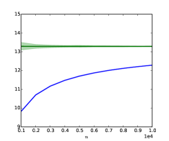
(a) Uniform

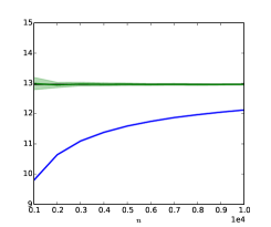
(b) Step

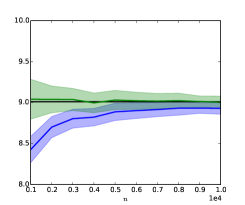
(c) Zipf with parameter $3/4$

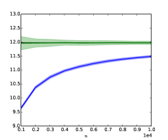
(d) Zipf with parameter $1/2$

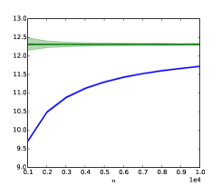
(e) Uniform prior (Dirichlet $1$)

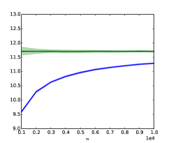
(f) Dirichlet $1/2$ prior

True value
Bias-corrected estimator
Empirical estimator estimator

Figure 2: Rényi entropy estimates for order $2$ for support $10000$, number of samples ranging from $1000$ to $10000$, averaged over $100$ trials.

(a) Uniform

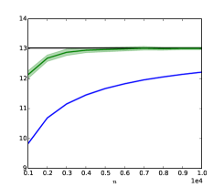
(b) Step

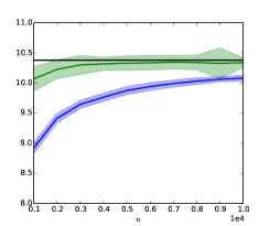
(c) Zipf with parameter $3/4$

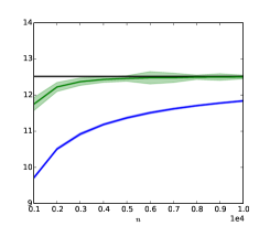
(d) Zipf with parameter $1/2$

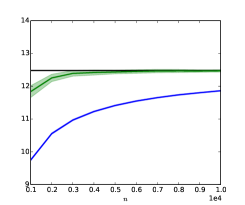
(e) Uniform prior (Dirichlet $1$)

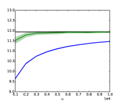
(f) Dirichlet $1/2$ prior

True value
Polynomial-approximation estimator
Empirical estimator estimator

Figure 3: Rényi entropy estimates for order $1.5$ for support $10000$, number of samples ranging from $1000$ to $10000$, averaged over $100$ trials.

V Lower bounds on sample complexity

We now establish lower bounds on $S_{\alpha}(k,\delta,\epsilon)$. The proof is based on exhibiting two distributions $\mathrm{p}$ and $\mathrm{q}$ with $H_{\alpha}(\mathrm{p})\neq H_{\alpha}(\mathrm{q})$ such that the set of $N_{x}$’s have very similar distribution from $\mathrm{p}$ and $\mathrm{q}$, if fewer samples than the claimed lower bound are available. This method is often referred to as Le Cam’s two-point method (see, for instance, [46]). The key idea is summarized in the following result which is easy to derive.

Lemma 15.

If for two distributions $\mathrm{p}$ and $\mathrm{q}$ on ${\mathcal{X}}$ and $n\in{\mathbbm{N}}$ the total variation distance $\|\mathrm{p}^{n}-\mathrm{q}^{n}\|<\epsilon$, then one of the following holds for every function $\hat{f}$:

$$\mathrm{p}\left(|H_{\alpha}(\mathrm{p})-\hat{f}(X^{n})|\geq\frac{|H_{\alpha}(\mathrm{p})-H_{\alpha}(\mathrm{q})|}{2}\right)\geq\frac{1-\epsilon}{2},$$

or $$\mathrm{q}\left(|H_{\alpha}(\mathrm{q})-\hat{f}(X^{n})|\geq\frac{|H_{\alpha}(\mathrm{p})-H_{\alpha}(\mathrm{q})|}{2}\right)\geq\frac{1-\epsilon}{2}.$$

We first prove the lower bound for integers $\alpha>1$, which matches the upper bound in Theorem 12 up to a constant factor.

Theorem 16.

Given an $1<\alpha\in{\mathbbm{N}}$ and $1<\epsilon<1$, for every sufficienly small $\delta>0$

$$S_{\alpha}(k,\delta,\epsilon)=\Omega\left(\frac{k^{(\alpha-1)/\alpha}}{\delta^{2}}\right),$$

where the constant implied by $\Omega$ may depend on $\epsilon$.

Proof.

We rely on Lemma 15 and exhibit two distributions $\mathrm{p}$ and $\mathrm{q}$ with appropriate properties. Specifically, consider the following distributions $\mathrm{p}$ and $\mathrm{q}$ over $[k]$: $\mathrm{p}_{1}=1/{k^{1-1/\alpha}}$, and for $x=2,\ldots,k$, $\mathrm{p}_{x}=(1-\mathrm{p}_{1})/(k-1)$; $\mathrm{q}_{1}=(1+\delta)/{k^{1-1/\alpha}}$, and for $x=2,\ldots,k$, $\mathrm{q}_{x}=(1-\mathrm{q}_{1})/(k-1)$. Then, we have

$${P}_{\alpha}(\mathrm{p}) =\frac{1}{k^{\alpha-1}}+(k-1)\cdot\left(\frac{1-\frac{1}{k^{1-1/\alpha}}}{k-1}\right)^{\alpha}$$

$$=\frac{1}{k^{\alpha-1}}+\frac{1}{(k-1)^{\alpha-1}}\cdot\left(1-\frac{1}{k^{1-1/\alpha}}\right)^{\alpha}$$

$$=\frac{(2+o_{k}(1))}{k^{\alpha-1}}.$$

Similarly,

$${P}_{\alpha}(\mathrm{q}) =\frac{(1+\delta)^{\alpha}}{k^{\alpha-1}}+(k-1)\cdot\left(\frac{1-\frac{(1+\delta)}{k^{1-1/\alpha}}}{k-1}\right)^{\alpha}$$

$$=\frac{(2+\alpha\delta+o_{k}(1))}{k^{\alpha-1}}.$$

Therefore, $|H_{\alpha}(\mathrm{p})-H_{\alpha}(\mathrm{q})|=\Omega(\delta)$. To complete the proof, we show that there exists a constant $C_{\epsilon}$ such that $\|\mathrm{p}^{n}-\mathrm{q}^{n}\|\leq\epsilon$ if $n\leq C_{\epsilon}k^{1-1/\alpha}/\delta^{2}$. To that end, we bound the squared Hellinger distance between $\mathrm{p}^{n}$ and $\mathrm{q}^{n}$ given by

$$h^{2}(\mathrm{p},\mathrm{q})=2-2\sum_{x}\sqrt{\mathrm{p}_{x}\mathrm{q}_{x}}=\sum_{x}(\sqrt{\mathrm{p}_{x}}-\sqrt{\mathrm{q}_{x}})^{2}.$$

Since for small values of $\delta$ we have $(1+\delta)^{1/2}<1+\delta$,

$$h^{2}(\mathrm{p},\mathrm{q}) =\left(\sqrt{\frac{1+\delta}{k^{1-1/\alpha}}}-\sqrt{\frac{1}{k^{1-1/\alpha}}}\right)^{2}+\left(\sqrt{1-\frac{1+\delta}{k^{1-1/\alpha}}}-\sqrt{1-\frac{1}{k^{1-1/\alpha}}}\right)^{2}$$

$$=O\left(\frac{\delta^{2}}{k^{1-1/\alpha}}\right).$$

The required bound for $\|\mathrm{p}^{n}-\mathrm{q}^{n}\|$ follows using the following standard steps ($cf.$ [46])

$$\|\mathrm{p}^{n}-\mathrm{q}^{n}\| \leq\sqrt{h^{2}(\mathrm{p},\mathrm{q})}$$

$$=\sqrt{1-\left(1-\frac{1}{2}h^{2}(\mathrm{p},\mathrm{q})\right)^{n}}$$

$$\leq\sqrt{\frac{n}{2}h^{2}(\mathrm{p},\mathrm{q})}.$$

∎

Next, we lower bound $S_{\alpha}(k)$ for noninteger $\alpha>1$ and show that it must be almost linear in $k$. While we still rely on Lemma 15 for our lower bound, we take recourse to Poisson sampling to simplify our calculations.

Lemma 17.

(Poisson approximation 2) Suppose there exist $\delta,\epsilon>0$ such that, with $N\sim{\rm Poi}(2n)$, for all estimators $\hat{f}$ we have

$$\max_{\mathrm{p}\in{\mathcal{P}}}{\mathbb{P}}\left(|H_{\alpha}(\mathrm{p})-\hat{f}_{\alpha}(X^{N})|>\delta\right)>\epsilon,$$

where ${\mathcal{P}}$ is a fixed family of distributions. Then, for all fixed length estimators $\tilde{f}$

$$\max_{\mathrm{p}\in{\mathcal{P}}}{\mathbb{P}}\left(|H_{\alpha}(\mathrm{p})-\tilde{f}_{\alpha}(X^{n})|>\delta\right)>\frac{\epsilon}{2},$$

when $n>4\log(2/\epsilon)$.

Also, it will be convenient to replace the observations $X^{N}$ with its profile $\Phi=\Phi(X^{N})$ [31], i.e., $\Phi=(\Phi_{1},\Phi_{2},\ldots)$ where $\Phi_{l}$ is the number of elements $x$ that appear $l$ times in the sequence $X^{N}$. The following well-known result says that for estimating $H_{\alpha}(\mathrm{p})$, it suffices to consider only the functions of the profile.

Lemma 18.

(Sufficiency of profiles). Consider an estimator $\hat{f}$ such that

$${\mathbb{P}}\left(|H_{\alpha}(\mathrm{p})-\hat{f}(X^{N})|>\delta\right)\leq\epsilon,\quad\text{for all }\mathrm{p}.$$

Then, there exists an estimator $\tilde{f}(X^{N})=\tilde{f}(\Phi)$ such that

$${\mathbb{P}}\left(|H_{\alpha}(\mathrm{p})-\tilde{f}(\Phi)|>\delta\right)\leq\epsilon,\quad\text{for all }\mathrm{p}.$$

Thus, lower bounds on the sample complexity will follow upon showing a contradiction for the second inequality above when the number of samples $n$ is sufficiently small. We obtain the required contradiction by using Lemma 15 upon showing there are distributions $\mathrm{p}$ and $\mathrm{q}$ of support-size $k$ such that the following hold:

• There exists $\delta>0$ such that

  $$|H_{\alpha}(\mathrm{p})-H_{\alpha}(\mathrm{q})|>\delta;$$ (20)

• denoting by $\mathrm{p}_{\Phi}$ and $\mathrm{q}_{\Phi}$, respectively, the distributions on the profiles under Poisson sampling corresponding to underlying distributions $\mathrm{p}$ and $\mathrm{q}$, there exist $\epsilon>0$ such that

  $$\|\mathrm{p}_{\Phi}-\mathrm{q}_{\Phi}\|<\epsilon,$$ (21)

  if $n<k^{\,c(\alpha)}$.

Therefore, it suffices to find two distributions $\mathrm{p}$ and $\mathrm{q}$ with different Rényi entropies and with small total variation distance between the distributions of their profiles, when $n$ is sufficiently small. For the latter requirement, we recall a result of [42] that allows us to bound the total variation distance in (21) in terms of the differences of power sums $|{P}_{a}(\mathrm{p})-{P}_{a}(\mathrm{q})|$.

Theorem 19.

[42] Given distributions $\mathrm{p}$ and $\mathrm{q}$ such that

$$\max_{x}\max\{\mathrm{p}_{x};\mathrm{q}_{x}\}\leq\frac{\epsilon}{40n},$$

for Poisson sampling with $N\sim{\rm Poi}(n)$, it holds that

$$\|\mathrm{p}_{\Phi}-\mathrm{q}_{\Phi}\|\leq\frac{\epsilon}{2}+5\sum_{a}n^{a}|{P}_{a}(\mathrm{p})-{P}_{a}(\mathrm{q})|.$$

It remains to construct the required distributions $\mathrm{p}$ and $\mathrm{q}$, satisfying (20) and (21) above. By Theorem 19, the total variation distance $\|\mathrm{p}_{\Phi}-\mathrm{q}_{\Phi}\|$ can be made small by ensuring that the power sums of distributions $\mathrm{p}$ and $\mathrm{q}$ are matched, that is, we need distributions $\mathrm{p}$ and $\mathrm{q}$ with different Rényi entropies and identical power sums for as large an order as possible. To that end, for every positive integer ${d}$ and every vector $\mathbf{x}=(x_{1},...,x_{d})\in{\mathbbm{R}}^{d}$, associate with $\mathbf{x}$ a distribution $\mathrm{p}^{\mathbf{x}}$ of support-size ${d}k$ such that

$$\mathrm{p}^{\mathbf{x}}_{ij}=\frac{|x_{i}|}{k\|\mathbf{x}\|_{1}},\quad 1\leq i\leq{d},\,1\leq j\leq k.$$

Note that

$$H_{\alpha}(\mathrm{p}^{\mathbf{x}}) =\log k+\frac{\alpha}{\alpha-1}\log\frac{\|\mathbf{x}\|_{1}}{\|\mathbf{x}\|_{\alpha}},$$

and for all $a$

$${P}_{a}\left(\mathrm{p}^{\mathbf{x}}\right) =\frac{1}{k^{a-1}}\left(\frac{\|\mathbf{x}\|_{a}}{\|\mathbf{x}\|_{1}}\right)^{a}.$$

We choose the required distributions $\mathrm{p}$ and $\mathrm{q}$, respectively, as $\mathrm{p}^{\mathbf{x}}$ and $\mathrm{p}^{\mathbf{y}}$, where the vectors $\mathbf{x}$ and $\mathbf{y}$ are given by the next result.

Lemma 20.

For every ${d}\in{\mathbbm{N}}$ and $\alpha$ not integer, there exist positive vectors $\mathbf{x},\mathbf{y}\in{\mathbbm{R}}^{d}$ such that

$$\|\mathbf{x}\|_{r} =\|\mathbf{y}\|_{r},\quad 1\leq r\leq{{d}-1},$$

$$\|\mathbf{x}\|_{d} \neq\|\mathbf{y}\|_{d},$$

$$\|\mathbf{x}\|_{\alpha} \neq\|\mathbf{y}\|_{\alpha}.$$

Proof.

Let $\mathbf{x}=(1,...,{d}))$. Consider the polynomial

$$p(z) =(z-x_{1})...(z-x_{d}),$$

and $q(z)=p(z)-\Delta$, where $\Delta$ is chosen small enough so that $q(z)$ has ${d}$ positive roots. Let $y_{1},...,y_{d}$ be the roots of the polynomial $q(z)$. By Newton-Girard identities, while the sum of ${d}$th power of roots of a polynomial does depend on the constant term, the sum of first ${d}-1$ powers of roots of a polynomial do not depend on it. Since $p(z)$ and $q(z)$ differ only by a constant, it holds that

$$\sum_{i=1}^{{d}}x_{i}^{r}=\sum_{i=1}^{{d}}y_{i}^{r},\quad 1\leq r\leq{d}-1,$$

and that

$$\sum_{i=1}^{{d}}x_{i}^{{d}}\neq\sum_{i=1}^{{d}}y_{i}^{d}.$$

Furthermore, using a first order Taylor approximation, we have

$$y_{i}-x_{i}=\frac{\Delta}{p^{\prime}(x_{i})}+o(\Delta),$$

and for any differentiable function $g$,

$$g(y_{i})-g(x_{i})=g^{\prime}(x_{i})(y_{i}-x_{i})+o(|y_{i}-x_{i}|).$$

It follows that

$$\sum_{i=1}^{d}g(y_{i})-g(x_{i})=\sum_{i=1}^{d}\frac{g^{\prime}(x_{i})}{p^{\prime}(x_{i})}\Delta+o(\Delta),$$

and so, the left side above is nonzero for all $\Delta$ sufficiently small provided

$$\sum_{i=1}^{d}\frac{g^{\prime}(x_{i})}{p^{\prime}(x_{i})}\neq 0.$$

Upon choosing $g(x)=x^{\alpha}$, we get

$$\sum_{i=1}^{d}\frac{g^{\prime}(x_{i})}{p^{\prime}(x_{i})}=\frac{\alpha}{{d}!}\sum_{i=1}^{d}\left(\begin{matrix}{d}\\ i\end{matrix}\right)(-1)^{{d}-i}\,i^{\alpha}.$$

Denoting the right side above by $h(\alpha)$, note that $h(i)=0$ for $i=1,...,{d}-1$. Since $h(\alpha)$ is a linear combination of ${d}$ exponentials, it cannot have more than ${d}-1$ zeros (see, for instance, [40]). Therefore, $h(\alpha)\neq 0$ for all $\alpha\notin\{1,...,{d}-1\}$; in particular, $\|\mathbf{x}\|_{\alpha}\neq\|\mathbf{y}\|_{\alpha}$ for all $\Delta$ sufficiently small. ∎

We are now in a position to prove our converse results.

Theorem 21.

Given a nonintegral $\alpha>1$, for any fixed $0<\epsilon<1/2$, we have

$$S_{\alpha}(k,\delta,\epsilon)=\stackrel{{\scriptstyle\sim}}{{\smash{\stackrel{{\scriptstyle\sim}}{{\smash{\Omega}\rule{0.0pt}{4.73611pt}}}}\rule{0.0pt}{6.45831pt}}}(k).$$

Proof.

For a fixed $d$, let distributions $\mathrm{p}$ and $\mathrm{q}$ be as in the previous proof. Then, as in the proof of Theorem 21, inequality (20) holds by Lemma 20 and (21) holds by Theorem 19 if $n<C_{2}k^{({d}-1)/{d}}$. The theorem follows since $d$ can be arbitrary large. ∎

Finally, we show that $S_{\alpha}(k)$ must be super-linear in $k$ for $\alpha<1$.

Theorem 22.

Given $\alpha<1$, for every $0<\epsilon<1/2$, we have

$$S_{\alpha}(k,\delta,\epsilon)=\stackrel{{\scriptstyle\sim}}{{\smash{\stackrel{{\scriptstyle\sim}}{{\smash{\Omega}\rule{0.0pt}{4.73611pt}}}}\rule{0.0pt}{6.45831pt}}}\left(k^{1/\alpha}\right).$$

Proof.

Consider distributions $\mathrm{p}$ and $\mathrm{q}$ on an alphabet of size $kd+1$, where

$$\mathrm{p}_{ij}=\frac{\mathrm{p}^{\mathbf{x}}_{ij}}{k^{\beta}}\text{ and }\mathrm{q}_{ij}=\frac{\mathrm{p}^{\mathbf{x}}_{ij}}{k^{\beta}},\quad 1\leq i\leq{d},\,1\leq j\leq k,$$

where the vectors $\mathbf{x}$ and $\mathbf{y}$ are given by Lemma 20 and $\beta$ satisfies $\alpha(1+\beta)<1$, and

$$\mathrm{p}_{0}=\mathrm{q}_{0}=1-\frac{1}{k^{\beta}}.$$

For this choice of $\mathrm{p}$ and $\mathrm{q}$, we have

$${P}_{a}\left(\mathrm{p}\right) =\left(1-\frac{1}{k^{\beta}}\right)^{a}+\frac{1}{k^{a(1+\beta)-1}}\left(\frac{\|\mathbf{x}\|_{a}}{\|\mathbf{x}\|_{1}}\right)^{a},$$

$$H_{\alpha}(\mathrm{p}) =\frac{1-\alpha(1+\beta)}{1-\alpha}\log k+\frac{\alpha}{1-\alpha}\log\frac{\|\mathbf{x}\|_{\alpha}}{\|\mathbf{x}\|_{1}}+O(k^{a(1+\beta)-1}),$$

and similarly for $\mathrm{q}$, which further yields

$$|H_{\alpha}(\mathrm{p})-H_{\alpha}(\mathrm{q})| =\frac{\alpha}{1-\alpha}\left|\log\frac{\|\mathbf{x}\|_{\alpha}}{\|\mathbf{y}\|_{\alpha}}\right|+O(k^{a(1+\beta)-1}).$$

Therefore, for sufficiently large $k$, (20) holds by Lemma 20 since $\alpha(1+\beta)<1$, and for $n<C_{2}k^{(1+\beta-1/d)}$ we get (21) by Theorem 19 as

$$\|\mathrm{p}_{\Phi}-\mathrm{q}_{\Phi}\|\leq\frac{\epsilon}{2}+5\sum_{a\geq{d}}\left(\frac{n}{k^{1+\beta-1/a}}\right)^{a}\leq\epsilon.$$

The theorem follows since $d$ and $\beta<1/\alpha-1$ are arbitrary. ∎

Appendix A: Estimating power sums

The broader problem of estimating smooth functionals of distributions was considered in [41]. Independently and concurrently with this work, [16] considered estimating more general functionals and applied their technique to estimating the power sums of a distribution to a given additive accuracy. Letting $S^{P+}_{\alpha}(k)$ denote the number of samples needed to estimate ${P}_{\alpha}(\mathrm{p})$ to a given additive accuracy, [16] showed that for $\alpha<1$,

$$S^{P+}_{\alpha}(k)=\Theta\left(\frac{k^{1/\alpha}}{\log k}\right),$$ (22)

and [17] showed that for $1<\alpha<2$,

$$S^{P+}_{\alpha}(k)\leq O\left(k^{2/\alpha-1}\right).$$

In fact, using techniques similar to multiplicative guarantees on ${P}_{\alpha}(\mathrm{p})$ we show that for $S^{P+}_{\alpha}(k)$ is a constant independent of $k$ for all $k>1$.

Since ${P}_{\alpha}(\mathrm{p})>1$ for $\alpha<1$, power sum estimation to a fixed additive accuracy implies also a fixed multiplicative accuracy, and therefore

$$S_{\alpha}(k)=\Theta(S^{P\times}_{\alpha}(k))\leq O(S^{P+}_{\alpha}(k)),$$

namely for estimation to an additive accuracy, Rényi entropy requires fewer samples than power sums. Similarly, ${P}_{\alpha}(\mathrm{p})<1$ for $\alpha>1$, and therefore

$$S_{\alpha}(k)=\Theta(S^{P\times}_{\alpha}(k))\geq\Omega(S^{P+}_{\alpha}(k)),$$

namely for an additive accuracy in this range, Rényi entropy requires more samples than power sums.

It follows that the power sum estimation results in [16, 17] and the Rényi-entropy estimation results in this paper complement each other in several ways. For example, for $\alpha<1$,

$$\stackrel{{\scriptstyle\sim}}{{\smash{\stackrel{{\scriptstyle\sim}}{{\smash{\Omega}\rule{0.0pt}{4.73611pt}}}}\rule{0.0pt}{6.45831pt}}}\left(k^{1/\alpha}\right)\leq S_{\alpha}(k)=\Theta(S^{P\times}_{\alpha}(k))\leq O(S^{P+}_{\alpha}(k))\leq O\left(\frac{k^{1/\alpha}}{\log k}\right),$$

where the first inequality follows from Theorem 22 and the last follows from the upper-bound (22) derived in [16] using a polynomial approximation estimator. Hence, for $\alpha<1$, estimating power sums to additive and multiplicative accuracy require a comparable number of samples.

On the other hand, for $\alpha>1$, Theorems 9 and  21 imply that for non integer $\alpha$, $\stackrel{{\scriptstyle\sim}}{{\smash{\stackrel{{\scriptstyle\sim}}{{\smash{\Omega}\rule{0.0pt}{4.73611pt}}}}\rule{0.0pt}{6.45831pt}}}\left(k\right)\leq S^{P\times}_{\alpha}(k)\leq O\left(k\right),$ while in the Appendix we show that for $1<\alpha$, $S^{P+}_{\alpha}(k)$ is a constant. Hence in this range, power sum estimation to a multiplicative accuracy requires considerably more samples than estimation to an additive accuracy.

We now show that the empirical estimator requires a constant number of samples to estimate ${P}_{\alpha}(\mathrm{p})$ independent of $k$, $i.e.$, $S^{P+}_{\alpha}(k)=O(1)$. In view of Lemma 8, it suffices to bound the bias and variance of the empirical estimator. Concurrently with this work, similar results were obtained in an updated version of [16].

As before, we comsider Poisson sampling with $N\sim{\rm Poi}(n)$ samples. The empirical or plug-in estimator of ${P}_{\alpha}(\mathrm{p})$ is

$$\widehat{P}_{\alpha}^{\text{e}}\stackrel{{\scriptstyle{\rm def}}}{{=}}\sum_{x}\left(\frac{N_{x}}{n}\right)^{\alpha}.$$

The next result shows that the bias and the variance of the empirical estimator are $o(1)$.

Lemma 23.

For an appropriately chosen constant $c>0$, the bias and the variance of the empirical estimator are bounded above as

$$\left|\widehat{P}_{\alpha}^{\text{e}}-{P}_{\alpha}(\mathrm{p})\right| \leq 2c\max\{n^{-(\alpha-1)},n^{-1/2}\},$$

$$\mathrm{\mathbb{V}ar}[{\widehat{\rm P}_{\alpha}}] \leq 2c\max\{n^{-(2\alpha-1)},n^{-1/2}\},$$

for all $n\geq 1$.

Proof.

Denoting $\lambda_{x}=n\mathrm{p}_{x}$, we get the following bound on the bias for an appropriately chosen constant $c$:

$$\left|\widehat{P}_{\alpha}^{\text{e}}-{P}_{\alpha}(\mathrm{p})\right| \leq\frac{1}{n^{\alpha}}\sum_{\lambda_{x}\leq 1}\left|\mathbb{E}\!\left[N_{x}^{\alpha}\,\right]-\lambda_{x}\right|+\frac{1}{n^{\alpha}}\sum_{\lambda_{x}>1}\left|\mathbb{E}\!\left[N_{x}^{\alpha}\,\right]-\lambda_{x}\right|$$

$$\leq\frac{c}{n^{\alpha}}\sum_{\lambda_{x}\leq 1}\lambda_{x}+\frac{c}{n^{\alpha}}\sum_{\lambda_{x}>1}\left(\lambda_{x}+\lambda_{x}^{\alpha-1/2}\right),$$

where the last inequality holds by Lemma 4 and Lemma 2since $x^{\alpha}$ is convex in $x$. Noting $\sum_{i}\lambda_{x}=n$, we get

$$\left|\widehat{P}_{\alpha}^{\text{e}}-{P}_{\alpha}(\mathrm{p})\right|\leq\frac{c}{n^{\alpha-1}}+\frac{c}{n^{\alpha}}\sum_{\lambda_{x}>1}\lambda_{x}^{\alpha-1/2}.$$

Similarly, proceeding as in the proof of Theorem 9, the variance of the empirical estimator is bounded as

$$\mathrm{\mathbb{V}ar}[{\widehat{\rm P}_{\alpha}}] =\frac{1}{n^{2\alpha}}\sum_{x\in{\mathcal{X}}}\mathbb{E}\!\left[N_{x}^{2\alpha}\,\right]-\mathbb{E}[N_{x}^{\alpha}]^{2}$$

$$\leq\frac{1}{n^{2\alpha}}\sum_{x\in{\mathcal{X}}}\left|\mathbb{E}\!\left[N_{x}^{2\alpha}\,\right]-\lambda_{x}^{2\alpha}\right|$$

$$\leq\frac{c}{n^{2\alpha-1}}+\frac{c}{n^{2\alpha}}\sum_{\lambda_{x}>1}\lambda_{x}^{2\alpha-1/2}.$$

The proof is completed upon showing that

$$\sum_{\lambda_{x}>1}\lambda_{x}^{\alpha-1/2}\leq\max\{n,n^{\alpha-1/2}\},\quad\alpha>1.$$

To that end, note that for $\alpha<3/2$

$$\sum_{\lambda_{x}>1}\lambda_{x}^{\alpha-1/2}\leq\sum_{\lambda_{x}>1}\lambda_{x}\leq n,\quad\alpha<3/2.$$

Further, since $x^{\alpha-1/2}$ is convex for $\alpha\geq 3/2$, the summation above is maximized when one of the $\lambda_{x}$’s is $n$ and the remaining equal $0$ which yields

$$\sum_{\lambda_{x}>1}\lambda_{x}^{\alpha-1/2}\leq n^{\alpha-1/2},\quad\alpha\geq 3/2,$$

and completes the proof. ∎

Appendix B: Lower bound for sample complexity of empirical estimator

We now derive lower bounds for the sample complexity of the empirical estimator of $H_{\alpha}(\mathrm{p})$.

Lemma 24.

Given $\alpha<1$ and $\delta<c_{\alpha}$ for a constant $c_{\alpha}$ depending only on $\alpha$, the sample complexity $S_{\alpha}^{f_{\alpha}^{\text{e}}}(k,\delta,\epsilon)$ of the empirical estimator $f_{\alpha}^{\text{e}}$ is bounded below as

$$S_{\alpha}^{f_{\alpha}^{\text{e}}}(k,\delta,0.9)=\Omega\left(\frac{k}{\delta}\right).$$

Proof.

We prove the lower bound for the uniform distributon over $k$ symbols in two steps. We first show that for any constant $c_{1}>1$ if $n<k/c_{1}$ then the additive approximation error is at least $\delta$ with probability one, for every $\delta<\log c_{1}$. Then, assuming that $n\geq k/c_{1}$, we show that the additve approximation error is at least $\delta$ with probability greater than $0.9$ if $n<k/\delta$.

For the first claim, we assume without loss of generality that $n\leq k$, since otherwise the proof is complete. Note that for $\alpha>1$ the function $(\mathrm{p}_{i}-y)^{\alpha}+(\mathrm{p}_{j}+y)^{\alpha}$ is decreasing in $y$ for all $y$ such that $(\mathrm{p}_{i}-y)>(\mathrm{p}_{j}+y)$. Thus, the minimum value of $\sum_{x}\left(\frac{N_{x}}{n}\right)^{\alpha}$ is attained when each $N_{x}$ is either $0$ or $1$. It follows that

$$\widehat{P}_{\alpha}^{\text{e}}=\sum_{x}\left(\frac{N_{x}}{n}\right)^{\alpha}\geq\frac{1}{n^{\alpha-1}},$$

which is the same as

$$H_{\alpha}(\mathrm{p})-\frac{1}{\alpha-1}\log\frac{1}{\widehat{P}_{\alpha}^{\text{e}}}\geq\log\frac{k}{n}.$$

Hence, for any $c_{1}>1$ and $n<k/c_{1}$ and any $0\leq\delta\leq\log c_{1}$, the additive approximation error is more than $\delta$ with probability one.

Moving to the second claim, suppose now $n>k/c_{1}$. We first show that with high probability, the multiplicities of a linear fraction of $k$ symbols should be at least a factor of standard deviaton higher than the mean. Specifically, let

$$A=\sum_{x}\mathds{1}\left(N_{x}\geq\frac{n}{k}+c_{2}\sqrt{\frac{n}{k}\left(1-\frac{1}{k}\right)}\right).$$

Then,

$$\mathbb{E}\!\left[A\,\right] =\sum_{x}\mathbb{E}\!\left[\mathds{1}\left(N_{x}\geq\frac{n}{k}+c_{2}\sqrt{\frac{n}{k}\left(1-\frac{1}{k}\right)}\right)\,\right]$$

$$=k\cdot p\left(N_{x}\geq\frac{n}{k}+c_{2}\sqrt{\frac{n}{k}\left(1-\frac{1}{k}\right)}\right)$$

$$\geq kQ(c_{2}),$$

where $Q$ denotes the $Q$-function, $i.e.$, the tail of the standard normal random variable, and the final inequality uses Slud’s inequality [38, Theorem 2.1].

Note that $A$ is a function of $n$ i.i.d. random variables $X_{1},X_{2},\ldots,X_{n}$, and changing any one $X_{i}$ changes $A$ by at most $2$. Hence, by McDiarmid’s inequality,

$$\Pr(A\geq\mathbb{E}\!\left[A\,\right]-\sqrt{8n})\geq 1-e^{-4}\geq 0.9.$$

Therefore, for all $k$ sufficiently large (depending on $\delta$) and denoting $c=Q(c_{2})/2$, at least $ck$ symbols occur more than $\frac{n}{k}+c_{2}\sqrt{\frac{n}{k}}$ times with probability greater than $0.9$. Using the fact that $(\mathrm{p}_{i}-y)^{\alpha}+(\mathrm{p}_{j}+y)^{\alpha}$ is decreasing if $(\mathrm{p}_{i}-y)>(\mathrm{p}_{j}+y)$ once more, we get

$$\sum_{x\in{\mathcal{X}}}\frac{N_{x}^{\alpha}}{n^{\alpha}} =\sum_{x:N_{x}\geq t}\frac{N_{x}^{\alpha}}{n^{\alpha}}+\sum_{x:N_{x}<t}\frac{N_{x}^{\alpha}}{n^{\alpha}}$$

$$\geq ck\left(\frac{1}{k}+c_{2}\sqrt{\frac{1}{nk}}\right)^{\alpha}+(1-c)k\left(\frac{1}{k}-\frac{cc_{2}}{1-c}\sqrt{\frac{1}{nk}}\right)^{\alpha}$$

$$=\frac{1}{k^{\alpha-1}}\left[c\left(1+c_{2}\sqrt{\frac{k}{n}}\right)^{\alpha}+(1-c)\left(1-\frac{cc_{2}}{1-c}\sqrt{\frac{k}{n}}\right)^{\alpha}\right]$$

$$\geq\frac{1}{k^{\alpha-1}}\left[c\left(1+c_{2}\sqrt{\frac{k}{n}}\right)^{\alpha}+(1-c)\left(1-\frac{\alpha cc_{2}}{1-c}\sqrt{\frac{k}{n}}\right)\right]$$

$$\geq\frac{1}{k^{\alpha-1}}\left[c\left(1+\alpha c_{2}\sqrt{\frac{k}{n}}+c_{4}\frac{k}{n}\right)+(1-c)\left(1-\frac{\alpha cc_{2}}{1-c}\sqrt{\frac{k}{n}}\right)\right]$$

$$=\frac{1}{k^{\alpha-1}}\left(1+cc_{4}\frac{k}{n}\right)$$

where the second inequality is by Bernoulli’s inequality and the third inequality holds for every $c_{4}\leq\alpha(\alpha-1)(c_{2}\sqrt{c_{1}})^{\alpha-2}/2$. Therefore, with probability $\geq 0.9$,

$$H_{\alpha}(\mathrm{p})-\frac{1}{\alpha-1}\log\frac{1}{\widehat{P}_{\alpha}^{\text{e}}}\geq\frac{1}{\alpha-1}\log\left(1+cc_{4}\frac{k}{n}\right),$$

which yields the desired bound. ∎

Lemma 25.

Given $\alpha<1$ and $\delta<c_{\alpha}$ for a constant $c_{\alpha}$ depending only on $\alpha$, the sample complexity $S_{\alpha}^{f_{\alpha}^{\text{e}}}(k,\delta,\epsilon)$ of the empirical estimator $f_{\alpha}^{\text{e}}$ is bounded as

$$S_{\alpha}^{f_{\alpha}^{\text{e}}}(k,\delta,0.9)=\Omega\left(\frac{k^{1/\alpha}}{\delta^{1/\alpha}}\right).$$

Proof.

We proceed as in the proof of the previous lemma. However, instead of using the uniform distribution, we use a distribution which has one “heavy element” and is uniform conditioned on the occurance of the remainder. The key observation is that there will be roughly $n^{\alpha}$ occurances of the “light elements”. Thus, when we account for the error in the estimation of the contribution of light elements to the power sum, we can replace $n$ with $n^{1/\alpha}$ in our analysis of the previous lemma, which yields the required bound for sample complexity.

Specifically, consider a distribution with one heavy element $0$ such that

$$\mathrm{p}_{0}=1-\frac{\delta}{n^{1-\alpha}},\,\,\text{ and }\,\,\mathrm{p}_{i}=\frac{\delta}{kn^{1-\alpha}},\quad 1\leq i\leq k.$$

Thus,

$${P}_{\alpha}(\mathrm{p})=\left(1-\frac{\delta}{n^{1-\alpha}}\right)^{\alpha}+\delta^{\alpha}\left(\frac{k}{n^{\alpha}}\right)^{1-\alpha}.$$ (23)

We begin by analyzing the estimate of the second term in power sum, namely

$$\sum_{i\in[k]}\left(\frac{N_{i}}{n}\right)^{\alpha}.$$

Let $R=\sum_{i\in[k]}N_{i}$ be the total number of occurances of light elements. Since $R$ is a binomial $(n,\delta n^{\alpha-1})$ random variable, for every constant $c>0$

$${\mathbb{P}}\left(1-c<\frac{R}{\delta n^{\alpha}}<1+c\right)\geq 1-\frac{1}{c^{2}n}.$$

In the remainder of the proof, we shall assume that this large probability event holds.

As in the proof of the previous lemma, we first prove a $\delta$ independent lower bound for sample complexity. To that end, we fix $\delta=1$ in the definition of $\mathrm{p}$. Assuming $(1+c)n^{\alpha}\leq k$, which implies $R\leq k$, and using the fact that $(\mathrm{p}_{i}-y)^{\alpha}-(\mathrm{p}_{j}+y)^{\alpha}$ is increasing in $y$ if $(\mathrm{p}_{i}-y)>(\mathrm{p}_{j}+y)$, we get

$$\widehat{P}_{\alpha}^{\text{e}} \leq 1+\left(\frac{R}{n}\right)^{\alpha}\sum_{i\in[k]}\left(\frac{N_{i}}{R}\right)^{\alpha}$$

$$\leq 1+\frac{(1+c)^{\alpha}}{n^{\alpha(1-\alpha)}}\sum_{i\in[k]}\left(\frac{N_{i}}{R}\right)^{\alpha}$$

$$\leq 1+\frac{(1+c)^{\alpha}}{n^{\alpha(1-\alpha)}}R^{1-\alpha}$$

$$\leq 3,$$

where the last inequality uses $R\leq(1+c)n^{\alpha}\leq 2n^{\alpha}$. Thus, the empirical estimate is at most $3$ with probability close to $1$ when $k$ (and therefore $n$) large. It follows from (23) that

$$H_{\alpha}(\mathrm{p})-\frac{1}{1-\alpha}\log{\widehat{P}_{\alpha}^{\text{e}}} \geq\log\frac{k}{3n^{\alpha}}.$$

Therefore, for all $c_{1}>1$, $\delta<\log 3c_{1}$ and $k$ sufficiently large, at least $\left(k/c_{1}\right)^{1/\alpha}$ samples are needed to get a $\delta$-additive approximation of $H_{\alpha}(\mathrm{p})$ with probability of error less than $1-1/({c^{2}n})$. Note that we only needed to assume $R\leq(10/9)n^{\alpha}$, an event with probability greater than $0.9$, to get the contradiction above. Thus, we may assume that $n\geq\left(k/c_{1}\right)^{1/\alpha}$. Under this assumption, for $k$ sufficiently large, $n$ is sufficiently large so that $(1-c)n^{\alpha}\leq R\leq(1+c)n^{\alpha}$ holds with probability arbitrarily close to $1$.

Next, assuming that $n\geq\left(k/c_{1}\right)^{1/\alpha}$, we obtain a $\delta$-dependent lower bound for sample complexity of the empirical estimator. We use the $\mathrm{p}$ mentioned above with a general $\delta$ and assume that the large probability event

$$(1-c)\leq\frac{R}{\delta n^{\alpha}}\leq(1+c)$$ (24)

holds. Note that conditioned on each value of $R$, the random variables $(N_{i},i\in[k])$ have a multinomial distribution with uniform probabilities, $i.e.$, these random variables behave as if we drew $R$ i.i.d. samples from a uniform distribution on $[k]$ elements. Thus, we can follow the proof of the previous lemma mutatis mutandis. We now define $A$ as

$$A=\sum_{x}\mathds{1}\left(N_{x}\leq\frac{n}{k}-c_{2}\sqrt{\frac{n}{k}\left(1-\frac{1}{k}\right)}\right).$$

and satisfies Then,

$$\mathbb{E}\!\left[A\,\right] =\sum_{x}\mathbb{E}\!\left[\mathds{1}\left(N_{x}\leq\frac{n}{k}-c_{2}\sqrt{\frac{n}{k}\left(1-\frac{1}{k}\right)}\right)\,\right]$$

$$=k\cdot p\left(N_{x}\leq\frac{n}{k}-c_{2}\sqrt{\frac{n}{k}\left(1-\frac{1}{k}\right)}\right).$$

To lower bound $p\left(N_{x}\leq\frac{n}{k}-c_{2}\sqrt{\frac{n}{k}\left(1-\frac{1}{k}\right)}\right)$ Slud’s inequality is no longer available (since it may not hold for ${\tt Bin}(n,p)$ with $p>1/2$ and that is the regime of interest for the lower tail probability bounds needed here). Instead we take recourse to a combination of Bohman’s inequality and Anderson-Samuel inequality, as suggested in [38, Eqns. (i) and (ii)]. It can be verified that the condition for [38, Eqns. (ii)] holds, and therefore,

$$p\left(N_{x}\leq\frac{n}{k}-c_{2}\sqrt{\frac{n}{k}\left(1-\frac{1}{k}\right)}\right)\geq Q(c_{2}).$$

Continuing as in the proof of the previous lemma, we get that the following holds with conditional probability greater than $0.9$ given each value of $R$ satisfying (24):

$$\sum_{i\in[k]}\left(\frac{N_{x}}{R}\right)^{\alpha} \leq k^{1-\alpha}\left(1-c_{3}\frac{k}{R}\right)$$

$$\leq k^{1-\alpha}\left(1-c_{4}\frac{k}{\delta n^{\alpha}}\right),$$

where $c_{3}$ is a sufficiently small constant such that $(1+x)^{\alpha}\leq 1+\alpha x-c_{3}x^{2}$ for all $x\geq 0$ and $c_{4}=c_{3}/(1+c)$. Thus,

$$\widehat{P}_{\alpha}^{\text{e}} \leq 1+\left(\frac{R}{n}\right)^{\alpha}\sum_{i\in[k]}\left(\frac{N_{i}}{R}\right)^{\alpha}$$

$$\leq 1+\left(\frac{R}{n}\right)^{\alpha}k^{1-\alpha}\left(1-c_{4}\frac{k}{\delta n^{\alpha}}\right)$$

$$\leq 1+\left(1+c\right)^{\alpha}\delta^{\alpha}\left(\frac{k}{n^{\alpha}}\right)^{1-\alpha}\left(1-c_{4}\frac{k}{\delta n^{\alpha}}\right).$$

Denoting $y=(k/n^{\alpha})$ and choosing $c_{1}$ and $c$ small enough such that $\widehat{P}_{\alpha}^{\text{e}}\leq 2$, for all sufficiently large $n$ we get from (23) that

$$\frac{{P}_{\alpha}(\mathrm{p})}{\widehat{P}_{\alpha}^{\text{e}}} \geq\frac{1-\delta+y^{1-\alpha}}{1+\delta^{\alpha}(1+c)^{\alpha}y^{1-\alpha}-(1+c)^{\alpha}c_{4}\delta^{\alpha-1}y^{2-\alpha}}$$

$$\geq\frac{1-\delta+y^{1-\alpha}}{1+y^{1-\alpha}-\delta^{\alpha-1}y^{2-\alpha}}$$

$$\geq 1-\frac{\delta}{2}+\frac{\delta^{\alpha-1}y^{2-\alpha}}{2},$$

where the second inequality uses the fact that $\delta^{\alpha}(1+c)^{\alpha}y^{1-\alpha}-(1+c)^{\alpha}c_{4}\delta^{\alpha-1}y^{2-\alpha}$ is negative, $c_{4}>1$ and $\delta<1$. Therefore, $\frac{{P}_{\alpha}(\mathrm{p})}{\widehat{P}_{\alpha}^{\text{e}}}\geq 1+\delta$ if $y^{2-\alpha}\geq 3\delta^{2-\alpha}$, which completes the proof. ∎

References

- [1] J. Acharya, A. Orlitsky, A. T. Suresh, and H. Tyagi, “The complexity of estimating rényi entropy,” in Proceedings of the Twenty-Sixth Annual ACM-SIAM Symposium on Discrete Algorithms, SODA 2015, San Diego, CA, USA, January 4-6, 2015, 2015, pp. 1855–1869.
- [2] A. Antos and I. Kontoyiannis, “Convergence properties of functional estimates for discrete distributions,” Random Struct. Algorithms, vol. 19, no. 3-4, pp. 163–193, Oct. 2001.
- [3] E. Arikan, “An inequality on guessing and its application to sequential decoding,” IEEE Transactions on Information Theory, vol. 42, no. 1, pp. 99–105, 1996.
- [4] Z. Bar-Yossef, R. Kumar, and D. Sivakumar, “Sampling algorithms: lower bounds and applications,” in Proceedings on 33rd Annual ACM Symposium on Theory of Computing, July 6-8, 2001, Heraklion, Crete, Greece, 2001, pp. 266–275.
- [5] T. Batu, L. Fortnow, R. Rubinfeld, W. D. Smith, and P. White, “Testing closeness of discrete distributions,” J. ACM, vol. 60, no. 1, p. 4, 2013.
- [6] C. Bennett, G. Brassard, C. Crepeau, and U. Maurer, “Generalized privacy amplification,” IEEE Transactions on Information Theory, vol. 41, no. 6, Nov 1995.
- [7] I. Csiszár, “Generalized cutoff rates and Renyi’s information measures,” IEEE Transactions on Information Theory, vol. 41, no. 1, pp. 26–34, Jan. 1995.
- [8] O. Goldreich and D. Ron, “On testing expansion in bounded-degree graphs,” Electronic Colloquium on Computational Complexity (ECCC), vol. 7, no. 20, 2000.
- [9] P. Grassberger, “Finite sample corrections to entropy and dimension estimates,” Physics Letters A, vol. 128, no. 6, pp. 369–373, 1988.
- [10] M. K. Hanawal and R. Sundaresan, “Guessing revisited: A large deviations approach,” IEEE Transactions on Information Theory, vol. 57, no. 1, pp. 70–78, 2011.
- [11] G. Hardy, J. E. Littlewood, and G. Pólya, Inequalities. 2nd edition. Cambridge University Press, 1952.
- [12] N. J. A. Harvey, J. Nelson, and K. Onak, “Sketching and streaming entropy via approximation theory,” in 49th Annual IEEE Symposium on Foundations of Computer Science, FOCS 2008, October 25-28, 2008, Philadelphia, PA, USA, 2008, pp. 489–498.
- [13] V. M. Ilic and M. S. Stankovic, “A unified characterization of generalized information and certainty measures,” CoRR, vol. abs/1310.4896, 2013. [Online]. Available: http://arxiv.org/abs/1310.4896
- [14] R. Impagliazzo and D. Zuckerman, “How to recycle random bits,” in FOCS, 1989.
- [15] R. Jenssen, K. Hild, D. Erdogmus, J. Principe, and T. Eltoft, “Clustering using Renyi’s entropy,” in Proceedings of the International Joint Conference on Neural Networks. IEEE, 2003.
- [16] J. Jiao, K. Venkat, Y. Han, and T. Weissman, “Minimax estimation of functionals of discrete distributions,” IEEE Transactions on Information Theory, vol. 61, no. 5, pp. 2835–2885, May 2015.
- [17] J. Jiao, K. Venkat, and T. Weissman, “Maximum likelihood estimation of functionals of discrete distributions,” CoRR, vol. abs/1406.6959, 2014.
- [18] D. Källberg, N. Leonenko, and O. Seleznjev, “Statistical inference for rényi entropy functionals,” CoRR, vol. abs/1103.4977, 2011.
- [19] D. E. Knuth, The Art of Computer Programming, Volume III: Sorting and Searching. Addison-Wesley, 1973.
- [20] A. Lall, V. Sekar, M. Ogihara, J. Xu, and H. Zhang, “Data streaming algorithms for estimating entropy of network traffic,” SIGMETRICS Perform. Eval. Rev., vol. 34, no. 1, pp. 145–156, Jun. 2006.
- [21] B. Ma, A. O. H. III, J. D. Gorman, and O. J. J. Michel, “Image registration with minimum spanning tree algorithm,” in ICIP, 2000, pp. 481–484.
- [22] Y. Mansour, M. Mohri, and A. Rostamizadeh, “Multiple source adaptation and the Renyi divergence,” CoRR, vol. abs/1205.2628, 2012.
- [23] V. Markov, “On functions deviating least from zero in a given interval,” Izdat. Imp. Akad. Nauk, St. Petersburg, pp. 218–258, 1892.
- [24] J. Massey, “Guessing and entropy,” in Information Theory, 1994. Proceedings., 1994 IEEE International Symposium on, Jun 1994, pp. 204–.
- [25] G. A. Miller, “Note on the bias of information estimates,” Information theory in psychology: Problems and methods, vol. 2, pp. 95–100, 1955.
- [26] A. Mokkadem, “Estimation of the entropy and information of absolutely continuous random variables,” IEEE Transactions on Information Theory, vol. 35, no. 1, pp. 193–196, 1989.
- [27] A. Motahari, G. Bresler, and D. Tse, “Information theory of dna shotgun sequencing,” Information Theory, IEEE Transactions on, vol. 59, no. 10, pp. 6273–6289, Oct 2013.
- [28] H. Neemuchwala, A. O. Hero, S. Z., and P. L. Carson, “Image registration methods in high-dimensional space,” Int. J. Imaging Systems and Technology, vol. 16, no. 5, pp. 130–145, 2006.
- [29] I. Nemenman, W. Bialek, and R. R. de Ruyter van Steveninck, “Entropy and information in neural spike trains: Progress on the sampling problem,” Physical Review E, vol. 69, pp. 056 111–056 111, 2004.
- [30] P. C. V. Oorschot and M. J. Wiener, “Parallel collision search with cryptanalytic applications,” Journal of Cryptology, vol. 12, pp. 1–28, 1999.
- [31] A. Orlitsky, N. P. Santhanam, K. Viswanathan, and J. Zhang, “On modeling profiles instead of values,” 2004.
- [32] L. Paninski, “Estimation of entropy and mutual information,” Neural Computation, vol. 15, no. 6, pp. 1191–1253, 2003.
- [33] ——, “Estimating entropy on m bins given fewer than m samples,” IEEE Transactions on Information Theory, vol. 50, no. 9, pp. 2200–2203, 2004.
- [34] ——, “A coincidence-based test for uniformity given very sparsely sampled discrete data,” vol. 54, no. 10, pp. 4750–4755, 2008.
- [35] C.-E. Pfister and W. Sullivan, “Renyi entropy, guesswork moments, and large deviations,” IEEE Transactions on Information Theory, vol. 50, no. 11, pp. 2794–2800, Nov 2004.
- [36] A. Rényi, “On measures of entropy and information,” in Proceedings of the Fourth Berkeley Symposium on Mathematical Statistics and Probability, Volume 1: Contributions to the Theory of Statistics, 1961, pp. 547–561.
- [37] P. S. Shenkin, B. Erman, and L. D. Mastrandrea, “Information-theoretical entropy as a measure of sequence variability,” Proteins, vol. 11, no. 4, pp. 297–313, 1991.
- [38] E. V. Slud, “Distribution Inequalities for the Binomial Law,” The Annals of Probability, vol. 5, no. 3, pp. 404–412, 1977.
- [39] A. F. Timan, Theory of Approximation of Functions of a Real Variable. Pergamon Press, 1963.
- [40] T. Tossavainen, “On the zeros of finite sums of exponential functions,” Australian Mathematical Society Gazette, vol. 33, no. 1, pp. 47–50, 2006.
- [41] G. Valiant and P. Valiant, “Estimating the unseen: an n/log(n)-sample estimator for entropy and support size, shown optimal via new clts,” 2011.
- [42] P. Valiant, “Testing symmetric properties of distributions,” in STOC, 2008.
- [43] Y. Wu and P. Yang, “Minimax rates of entropy estimation on large alphabets via best polynomial approximation,” CoRR, vol. abs/1407.0381v1, 2014.
- [44] D. Xu, “Energy, entropy and information potential for neural computation,” Ph.D. dissertation, University of Florida, 1998.
- [45] D. Xu and D. Erdogmuns, “Renyi’s entropy, divergence and their nonparametric estimators,” in Information Theoretic Learning, ser. Information Science and Statistics. Springer New York, 2010, pp. 47–102.
- [46] B. Yu, “Assouad, Fano, and Le Cam,” in Festschrift for Lucien Le Cam. Springer New York, 1997, pp. 423–435.