Finite-$N$ corrections to Vlasov dynamics and the range of pair interactions

Abstract

Abstract

We explore the conditions on a pair interaction for the validity of the Vlasov equation to describe the dynamics of an interacting $N$ particle system in the large $N$ limit. Using a coarse-graining in phase space of the exact Klimontovich equation for the $N$ particle system, we evaluate, neglecting correlations of density fluctuations, the scalings with $N$ of the terms describing the corrections to the Vlasov equation for the coarse-grained one particle phase space density. Considering a generic interaction with radial pair force $F(r)$, with $F(r)\sim 1/r^{\gamma}$ at large scales, and regulated to a bounded behaviour below a “softening” scale $\varepsilon$, we find that there is an essential qualitative difference between the cases $\gamma<d$ and $\gamma>d$, i.e., depending on the integrability at large distances of the pair force. In the former case the corrections to the Vlasov dynamics for a given coarse-grained scale are essentially insensitive to the softening parameter $\varepsilon$, while for $\gamma>d$ the amplitude of these terms is directly regulated by $\varepsilon$, and thus by the small scale properties of the interaction. This corresponds to a simple physical criterion for a basic distinction between long-range ($\gamma\leq d$) and short range ($\gamma>d$) interactions, different to the canonical one ($\gamma\leq d+1$ or $\gamma>d+1$ ) based on thermodynamic analysis. This alternative classification, based on purely dynamical considerations, is relevant notably to understanding the conditions for the existence of so-called quasi-stationary states in long-range interacting systems.

today

Interactions are canonically characterized as short-range or long-range on the basis of the fundamental distinction which arises in equilibrium statistical mechanics between interactions for which the energy is additive and those for which it is non-additive (for reviews, see e.g. (Campa2009, ; Dauxois2002, ; Campa2008, ; Bouchet2010, )). For a system of particles interacting via two body interactions with a pair potential $V(r)$, the system is then long-range (or “strongly long range” (Bouchet2010, ) ) if and only if $V(r)$ decays at large distances slower than one over the separation $r$ to the power of the spatial dimension $d$. In the last decade there has been considerable study of this class of interactions. One of the very interesting results about systems in this class which has emerged — essentially through numerical study of different models — is that, like for the much studied case of gravity in astrophysics, their dynamics leads, from generic initial conditions, to so-called quasi-stationary states: macroscopic non-equilibrium states which evolve only on timescales which diverge with particle number. Theoretically these states are interpreted in terms of a description of the system’s dynamics by the Vlasov equation, of which they represent stationary solutions. Their physical realizations arise in numerous and very diverse systems, ranging from galaxies and “dark matter halos” in astrophysics and cosmology (see e.g. Binney2008 ) to the red spot on Jupiter (see e.g. Bouchet2002 ), to laboratory systems such as cold atoms Olivetti2009 , and even to biological systemsSopik2005 . A basic question is whether the appearance of these out of equilibrium stationary states — and more generally the validity of the Vlasov equation to describe the system’s dynamics — applies to the same class of long-range interactions as defined by equilibrium statistical mechanics, or only to a sub-class of them, or indeed to a larger class of interactions. In short, in what class of systems can we expect to see these quasi-stationary states? Are they typical of long-range interactions as defined canonically? Or are they characteristic of a different class?

To answer these questions requires establishing the conditions of validity of the Vlasov equation, and specifically how such conditions depend on the two-body interaction. In the literature there are, on the one hand, some rigourous mathematical results establishing sufficient conditions for the existence of the Vlasov limit. It has been proven notably (Braun1977, ; Spohn1991, ; Hauray2007, ) that the Vlasov equation is valid on times scales of order $\sim logN$ times the dynamical time, for strictly bound pair potentials decaying at large separations $r$ slower than $r^{-(d-2)}$. On the other hand, both results of numerical study and various theoretical approaches, based on different approximations or assumptions, suggest that much weaker conditions are sufficient, and the timescales for the validity of the Vlasov equation can be much longer. In the much studied case of gravity, notably, a treatment originally introduced by Chandrasekhar, (Chandrasekhar1943, ) and subsequently refined by other authors (see e.g. (Henon1958, ; Chavanis2010, ; Farouki1994, ; Farouki1982, )) in which non-Vlasov effects are assumed to be dominated by incoherent two body interactions gives a time scale $\sim N/logN$ times the dynamical time for the validity of the Vlasov equation, at least close to stationary solutions representing quasi-stationary states, and this in absence of a regularisation of the singularity in the two-body potential. Theoretical approaches in the physics literature derive the Vlasov equation and kinetic equations describing corrections to it (for a review see(Campa2009, ; Chavanis2012a, ) either within the framework of the BBGKY hierarchy(balescu1975, ) or starting from the exact Klimontovich equation for the N body system (Klimontovich1967, ; Nicholson1983, )). These approaches are both widely argued (see e.g. (Chavanis2012a, ; Chavanis2013, ; Campa2009, ; Bouchet2010, ; Filho2012, )), to lead generally to lifetimes of quasi-stationary states of order $\sim N$ times the dynamical time for any softened pair potential , except in the special case of spatially homogeneous quasi-stationary states one dimension.

In this article we address the question of the validity of Vlasov dynamics using an approach starting from the exact Klimontovich equation. Instead of considering, as is often done (see e.g. Campa2009 ; Chavanis2012a ; Bouchet2010 ), an average over an ensemble of initial conditions to define a smooth one particle phase density, we follow an approach (described e.g. in Buchert2005 ) in which such a smoothed density is obtained by performing a coarse-graining in phase space. This approach gives the Vlasov equation for the coarse-grained phase space density when certain terms are discarded. We then study how the latter “non-Vlasov” terms depend on the particle number $N$, and on the scales introduced by the coarse-graining. In particular we develop this study analyzing the dependence on the large and small distance behavior of the two body potential. Our analysis leading to the scaling behaviours of these terms is based only one very simple — but physically reasonable — hypothesis that we can neglect all correlations in the (microscopic) $N$ body configurations other than those coming from the mean (coarse-grained) phase space density. The main physical result we highlight is that, under this simple hypothesis, the coarse-grained dynamics of an interacting $N$-particle system shows a very different dependence on the pair interaction at small scale depending on how fast the interaction decays at large distances: for interactions of which the pair force is integrable at large scales the coarse-grained $N$ body dynamics is highly sensitive to how the potential is softened at much smaller scales, while for pair forces which are non-integrable the opposite is true. Correspondingly, while the Vlasov limit may be obtained for any pair interaction which is softened suitably at small scales, the conditions on the short-scale behaviour of the interaction are very different depending on whether its large scale behaviour is in one of of these two classes. This result provides a more rigorous basis for a “dynamical classification” of interactions as long-range or short-range, which has been introduced on the basis of simple considerations of the probability distribution of the force on a random particle in a uniform particle distribution in (Gabrielli2010, ), and found also in (Gabrielli2010a, ) to coincide with a classification based on the dependence on softening of collisional time scales using a generalisation of the analysis of Chandrasekhar for the case of gravity.

The article is organized as follows. In the next section we derive the equation for the coarse-grained phase space density and write in a simple form the non-Vlasov terms which our subsequent analysis focusses on. In section II we first explain our central hypothesis concerning the $N$-body dynamics, and then apply it to evaluate the statistical properties of the non-Vlasov terms. In the following section we then determine the scaling behaviours of these expressions, i.e., how they depend parametrically on the relevant parameters introduced, and in particular on the two parameters characterising the two body interaction — its large scale decay and the scale at which it is softened. In section IV we use these expressions to identify the dominant contributions to the non-Vlasov terms, which turn out to differ depending on how rapidly the interaction decays at large scales. In the following section we present more complete exact results for the one dimensional case and the comparison with a simple numerical simulation. We then summarize our results and conclusions, discussing in particular the central assumptions and the dependence of our findings on them.

I A Vlasov-like equation for the coarse-grained phase space density

In this section we summarize an approach used to justify the validity of the Vlasov equation for long-range interacting systems. The approach involves using a coarse-graining, in phase space, of the full N body dynamics and leads to an evolution equation for the coarse grained phase space density which consists of the Vlasov terms, plus additional terms. This equation, and the specific form of the non-Vlasov terms we derive, is the starting point for our analysis in the subsequent sections. We follow closely at the beginning the presentation and notation of Buchert2005 .

We consider a $d$-dimensional system of $N$ particles of identical mass $m=1$ interacting only through the a generic two body force, denoting ${\mathbf{g}}({\bf x})$ the force on a particle at ${\bf x}$ exerted by another one at the origin.

At any time $t$, the $N$ particles have phase space positions which we denote $\{({\bf x}_{i},{\bf v}_{i})\}_{i=1..N}$, and the microscopic (or fine-grained, or Klimontovich) one particle phase-space density is simply the distribution

$$f_{k}({\bf x},{\bf v},t)=\sum_{i=1}^{N}\delta({\bf x}-{\bf x}_{i}(t))\delta({\bf v}-{\bf v}_{i}(t))\,.$$ (1)

Likewise the microscopic density in one particle coordinate space is

$$n_{k}({\bf x})=\int f_{k}d^{d}{\bf v}=\sum_{i=1}^{N}\delta({\bf x}-{\bf x}_{i})$$ (2)

The full evolution of the $N$ body system can be written in the form of the so-called Klimontovich equation for the microscopic phase space density:

$$\frac{\partial f_{k}}{\partial t}+{\bf v}\frac{\partial f_{k}}{\partial{\bf x}}+{\mathbf{F}}[n_{k}]({\bf x})\frac{\partial f_{k}}{\partial{\bf v}}=0.$$ (3)

where

$${\mathbf{F}}[n_{k}]({\bf x})=\int_{\Omega}{\mathbf{g}}({\bf x}-{\bf x}^{\prime})n_{k}({\bf x}^{\prime})d^{d}{\bf x}^{\prime}=\sum_{i=1}^{N}{\mathbf{g}}({\bf x}-{\bf x}_{i})$$ (4)

is the exact force at point $x$ (due to all other particles). The only assumption made in deriving this equation from the equations of motion of the individual particles is that the force ${\mathbf{g}}({\bf x})$ is bounded as $x\rightarrow 0$.

Introducing a top-hat window function $W({\bf z}=z_{1},\dots,z_{d})$,

$$W(z_{1},\dots,z_{d})=\left\{\begin{array}[]{ll}1,&\,{\rm if}\,|z_{i}|<\frac{1}{2},\,\forall i=1\dots d\\ 0&{\rm otherwise}\end{array}\right.$$ (5)

we define the coarse-grained phase space density:

$$f_{0}({\bf x},{\bf v},t)\!=\!\!\!\int\!\!\frac{d^{d}{\bf x}^{\prime}}{\lambda_{x}^{d}}\frac{d^{d}{\bf v}^{\prime}}{\lambda_{v}^{d}}W\!\!\left(\!\frac{{\bf x}-{\bf x}^{\prime}}{\lambda_{x}}\!\right)\!\!W\!\!\left(\!\frac{{\bf v}-{\bf v}^{\prime}}{\lambda_{v}}\!\right)\!\!f_{k}({\bf x}^{\prime}\!,{\bf v}^{\prime}\!,t)$$ (6)

where $\lambda_{x}$ and $\lambda_{v}$ are the characteristic sizes of the coarse-graining cell in position and, respectively, velocity space. We will denote by $\mathcal{C}({\bf x},{\bf v})$ the coarse graining cell centred at $({\bf x},{\bf v})$, which thus has a phase space volume $\lambda_{x}^{d}\,\lambda_{v}^{d}$, and

$$N_{c}({\bf x},{\bf v},t)=\lambda_{x}^{d}\lambda_{v}^{d}f_{0}({\bf x},{\bf v},t)$$ (7)

is the number of particles in $\mathcal{C}({\bf x},{\bf v})$. We suppose that the coarse graining cell is always much smaller (in both real and velocity space) than the characteristic size of the system, but sufficiently large to contain a large number of particles, i.e., $\lambda_{x}\ll L_{x}$ and $\lambda_{v}\ll L_{v}$ where $L_{x}$ and $L_{v}$ the characteristic size of the system in coordinate and velocity space respectively, and

$$1\ll N_{c}({\bf x},{\bf v},t)\ll N\,.$$ (8)

We define also the coarse-grained spatial density as

$$n_{0}({\bf x},t)=\int d^{d}{\bf v}f_{0}({\bf x},{\bf v},t)=\int\frac{d^{d}x^{\prime}}{\lambda_{x}}W\left(\frac{{\bf x}-{\bf x}^{\prime}}{\lambda_{x}}\right)n_{k}({\bf x}^{\prime})$$ (9)

By integrating Eq. (3) over the coarse-graining cell we obtain straightforwardly the following equation:

$$\frac{\partial f_{0}}{\partial t}+{\bf v}\cdot\frac{\partial f_{0}}{\partial{\bf x}}+{\mathbf{F}}_{0}({\bf x})\cdot\frac{\partial f_{0}}{\partial{\bf v}}\!=\!-\frac{\partial}{\partial{\bf x}}[f_{0}\,\xi_{{\bf v}}]-\frac{\partial}{\partial{\bf v}}[f_{0}\,\xi_{{\mathbf{F}}}]$$ (10)

where

$${\mathbf{F}}_{0}({\bf x},t)=\int_{\Omega}{\mathbf{g}}({\bf x}-{\bf x}^{\prime})n_{0}({\bf x}^{\prime},t)d^{d}{\bf x}^{\prime}\,,$$ (11)

i.e., the force at the point ${\bf x}$ due to the coarse-grained distribution (which we will identify as the mean-field force). Furthermore

$$\xi_{v}({\bf x},{\bf v},t)=\left[\frac{1}{N_{c}({\bf x},{\bf v},t)}\sum_{i\in\mathcal{C}({\bf x},{\bf v})}{\bf v}_{i}(t)\right]-{\bf v}\,$$ (12)

where ${\bf v}_{i}$ is the velocity of particle $i$, and

$$\xi_{{\mathbf{F}}}({\bf x},{\bf v},t)=\left[\frac{1}{N_{c}({\bf x},{\bf v},t)}\sum_{i\in\mathcal{C}({\bf x},{\bf v})}{\mathbf{F}}_{i}(t)\right]-{\mathbf{F}}_{0}({\bf x},t)$$ (13)

where ${\mathbf{F}}_{i}$ is the exact force acting on the particle $i$, i.e., ${\mathbf{F}}_{i}={\mathbf{F}}({\bf x}_{i},t)$ where

$${\mathbf{F}}({\bf x},t)=\int_{\Omega}{\mathbf{g}}({\bf x}-{\bf x}^{\prime})n_{k}({\bf x}^{\prime},t)d^{d}{\bf x}^{\prime}\,.$$ (14)

Thus $\xi_{\bf v}$ is the “velocity fluctuation” in the cell $({\bf x},{\bf v})$ around the coarse-grained velocity ${\bf v}$, i.e., difference between the arithmetic mean of particles velocities in the cell (i.e. the velocity of the center of mass) and the velocity at the centre of the coarse-graining cell, and $\xi_{{\mathbf{F}}}({\bf x},{\bf v},t)$ is the “force fluctuation” around the coarse-grained force, i.e., the difference between the arithmetic mean of the exact forces acting on each particle in the cell (equal to the force on the centre of mass of the particles in the cell) and the force at the centre of the cell due to the coarse-grained particle distribution.

If the right hand side of Eq. (10) is set equal to zero, we obtain, given Eq. (11), the Vlasov equation for the coarse-grained phase space density $f_{0}({\bf x},{\bf v},t)$. Establishing the validity of the Vlasov equation in an appropriate limit thus requires showing that the terms on the right-hand side may indeed be taken to zero in this limit. For a real system, for which $N$ is finite and the typical number of particles in a coarse-graining cell is finite, Eq. (10) is not closed for the coarse-grained phase space density, but rather coupled to the fine-grained density through the terms on the right-hand side. If it is possible to define the Vlasov limit for the system, these terms will represent at any finite (but large) $N$, small perturbations to the pure Vlasov evolution of the coarse-grained distribution associated with the “graininess” of the system which, under suitable hypothesis, are responsible for the relaxation of the system to the thermodynamic equilibrium. In the rest of this article we focus on these terms, and establish their scaling with $N$ (or, equivalently, as a function of the characteristic scales of the coarse-graining cell), given certain simplifying hypotheses.

II Statistical evaluation of the finite-$N$ fluctuating terms

We now focus on the two terms on the right-hand side of Eq. (10). Their direct evaluation is clearly impossible as in principle it requires knowledge of the full fine-grained phase space density. We can, however, determine how they scale as a function of relevant parameters by using a statistical approach: given a coarse-grained distribution $f_{0}({\bf x},{\bf v})$ we can consider the fine-grained distribution to be characterized by an ensemble of realizations of particle distributions having $f_{0}({\bf x},{\bf v})$ as mean density. If we know the statistical properties of this ensemble, we can then, in principle, calculate those of the fluctuating terms on the right-hand side of Eq. (10). In particular, we can then consider how the amplitudes of these statistical quantities depend on the relevant parameters.

We make here the most simple possible hypothesis about this ensemble for the fine-grained phase space density: we suppose that it corresponds to the ensemble of realizations of an inhomogeneous Poissonian point process with mean density given by the coarse-grained phase space density $f_{0}({\bf x},{\bf v})$. In other words we assume that the particles are randomly distributed, without any correlation, inside each coarse-grained cell, with a mean density which varies from cell to cell following $f_{0}({\bf x},{\bf v})$. The density-density correlations are thus fully described by the one point distribution $f_{0}({\bf x},{\bf v})$, and all other correlations, of the fluctuations around this mean density, are neglected. Physically this means we retain the “pure” finite $N$ (discreteness) effects arising from the fluctuations of the mean density, but neglect the correlation of these fluctuations. Alternatively one can consider that we proceed by assuming complete ignorance of the distribution of particles below the coarse-graining scale, other than the information furnished about it by the coarse-grained density itself. This allows us in effect to close, at least in a statistical formulation, Eq. (10) for $f_{0}({\bf x},{\bf v})$. Indeed this hypothesis is arguably the most natural one to make in seeking to obtain a criterion for the validity of the Vlasov equation which is based only on the coarse graining density $f_{0}({\bf x},{\bf v})$ and the properties of the pair interaction itself.

Formally we can state our assumption to be that the relevant terms can be evaluated by considering an ensemble of realizations of a point process with the N particle probability distribution in phase space given by (see, e.g., gabrielli2006statistical )

$$\mathcal{P}_{N}({\bf x}_{1},{\bf v}_{1};..;{\bf x}_{N},{\bf v}_{N})=\prod^{N}_{i=1}\frac{f_{0}({\bf x}_{i},{\bf v}_{i})}{N}$$ (15)

assuming the coarse-grained phase space density $f_{0}({\bf x},{\bf v})$ to be a smooth function. In practice it is convenient to perform the calculation with finite coarse-grained cells in which $f_{0}({\bf x},{\bf v})$ is fixed, and the particles are distributed randomly in each coarse-grained cell.

II.1 Mean and variance of $\xi_{\bf v}$

We first evaluate the mean and variance of $\xi_{v}$, as defined by Eq. (12), assuming now the defined properties of the ensemble of realizations. Given that the latter assigns randomly the velocities of the particles in the coarse-grained cell, which is centred at $({\bf x},{\bf v})$, we evidently have

$$\left<\frac{1}{N_{c}({\bf x},{\bf v},t)}\sum_{i\in\mathcal{C}({\bf x},{\bf v})}{\bf v}_{i}(t)\right>={\bf v}\,,$$ (16)

where $\left<...\right>$ denotes the ensemble average. Therefore we have, as would be expected,

$$\left<\xi_{{\bf v}}\right>=0\,.$$ (17)

Calculating the variance of $\xi_{{\bf v}}$ gives straightforwardly that

$$\left<\xi_{{\bf v}}^{2}\right>=\frac{1}{N_{c}({\bf x},{\bf v})}\frac{d}{12}\lambda_{v}^{2}$$ (18)

where we can take $N_{c}=f_{0}({\bf x},{\bf v})\lambda_{x}^{d}\lambda_{v}^{d}$ to be the average number of particles in the cell, given that $N_{c}=\left<N_{c}\right>+\delta N_{c}$ where by hypothesis $\delta N_{c}\sim\sqrt{N_{c}}\ll N_{c}$ . Given that $N_{c}({\bf x},{\bf v})$ is large, and ${\bf v}_{i}$ are considered independent and identically distributed variables, $\xi_{{\bf v}}$ is thus simply a Gaussian random variable with mean zero and variance given by Eq. (18).

II.2 Mean and variance of $\xi_{\mathbf{F}}$

Let us evaluate now the first two moments of $\xi_{{\mathbf{F}}}$. To evaluate these quantities in the ensemble defined above, it is useful first to note that

$$\bar{{\mathbf{F}}}({\bf x},{\bf v},t) \doteq\frac{1}{N_{c}({\bf x},{\bf v},t)}\sum_{i\in\mathcal{C}({\bf x},{\bf v})}{\mathbf{F}}_{i}(t)$$ (19)

$$=\frac{1}{N_{c}}\sum_{i=1}^{N_{c}}\sum_{I=1}^{N-N_{c}}{\mathbf{g}}({\bf x}_{i}-{\bf y}_{I})$$

where the $i$ runs over the $N_{c}$ particles inside the coarse-graining cell $\mathcal{C}({\bf x},{\bf v})$, and the index $I$ over the other $N-N_{c}$ particles outside the cell. This is the case because we assume ${\mathbf{g}}(-{\bf x})=-{\mathbf{g}}({\bf x})$ (making the sum over all the mutual forces of the pairs of particles in the cell $\mathcal{C}({\bf x},{\bf v})$ vanishes). As the individual pair forces depend only on the spatial positions of particles, we need only specify, to calculate the ensemble average of powers of the force, the probability distribution for the spatial positions of these points. Given the writing of the force in (19), in which the sum is performed separately over the particles inside and outside the coarse-grained cell $\mathcal{C}({\bf x},{\bf v})$ considered, it is convenient to write the ensemble average in a similar form. As noted above we can take $N_{c}$ to be fixed and equal to its average value, $n_{0}({\bf x})\lambda_{x}^{d}$, up to negligible corrections of order $1/\sqrt{N_{c}}$. We can then write the N particle probability distribution as

$$\mathcal{P}_{N}^{\,\prime}({\bf x}_{1},..{\bf x}_{N_{c}};{\bf y}_{1},..{\bf y}_{N-N_{c}})=\prod^{N_{c}}_{i=1}p({\bf x}_{i})\prod^{N-N_{c}}_{I=1}\hat{p}({\bf y}_{I})$$ (20)

where $p({\bf x})$ is the one-point probability distribution function of the spatial position of a particle given the condition that it is contained in the cell, and $\hat{p}({\bf y})$ is the one-point probability distribution of the spatial position of a particle given the condition that it is outside the cell. Given that the $N_{c}$ particles are randomly distributed inside the cell, we have simply

$$p({\bf x}_{i})=\left\{\begin{array}[]{ll}\lambda_{x}^{-d},&{\bf x}\in\mathcal{S}({\bf x})\\ 0,&{\rm otherwise}\end{array}\right.$$ (21)

where $\mathcal{S}({\bf x})$ is the support of $W({\bf x}/\lambda_{x})$, i.e., the “stripe” in phase space with the same spatial coordinates as the phase space cell $\mathcal{C}({\bf x},{\bf v})$ (see Fig. 1). Assuming the number of particles in the cell $N_{c}$ to be small compared to the total number of particles $N_{s}({\bf x},{\bf v})$ in this stripe (which is itself small compared to the total number of particles $N$), $\hat{p}({\bf y})$ can be approximated everywhere simply by the unconditional one point PDF for the spatial distribution obtained by integrating (15) over all but one space coordinate, i.e.,

$$\hat{p}({\bf y})=\frac{n_{0}({\bf y})}{N}$$ (22)

II.2.1 Mean of $\xi_{{\mathbf{F}}}$

Using (20) to calculate the ensemble average of the exact force exerted by all particles on those in a coarse-grained cell, we have

$$\left<\bar{{\mathbf{F}}}({\bf x},{\bf v},t)\right> = (N-N_{c})\int_{\Omega}d^{d}{\bf x}^{\prime}\int_{\Omega}d^{d}y^{\prime}p({\bf x}^{\prime})\hat{p}({\bf y}^{\prime}){\mathbf{g}}({\bf x}^{\prime}-{\bf y}^{\prime})$$ (23)

$$= \int_{\mathcal{S}({\bf x})}\frac{d^{d}{\bf x}^{\prime}}{\lambda_{x}^{d}}\int_{\Omega}d^{d}{\bf y}^{\prime}n_{0}({\bf y}^{\prime}){\mathbf{g}}({\bf x}^{\prime}-{\bf y}^{\prime})$$

$$= \int_{\mathcal{S}({\bf x})}\frac{d^{d}{\bf x}^{\prime}}{\lambda_{x}^{d}}{\mathbf{F}}_{0}({\bf x}^{\prime})$$

Thus

$$\left<\xi_{{\mathbf{F}}}({\bf x},{\bf v},t)\right>=\int_{\mathcal{S}({\bf x})}\frac{d^{d}{\bf x}^{\prime}}{\lambda_{x}^{d}}[{\mathbf{F}}_{0}({\bf x}^{\prime})-{\mathbf{F}}_{0}({\bf x})]\,.$$ (24)

Assuming that we can neglect the variation of the mean-field ${\mathbf{F}}_{0}$ in the coarse-graining cell, we obtain

$$\left<\xi_{{\mathbf{F}}}({\bf x},{\bf v},t)\right>=0$$ (25)

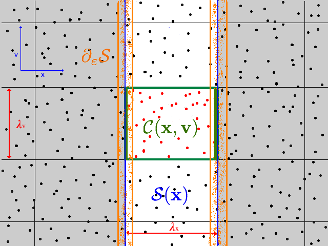
Figure 1: (Color online) Schema, in one dimension, of the coarse-graining of phase space, showing also the different regions into which the domain of integration is divided for our analysis of the integrals in the force variance: $\mathcal{C}$ is the coarse-grained cell with centre at $({\bf x},{\bf v})$, $\mathcal{S}$ (in white) is the “stripe” enclosing all points in $[{\bf x}-\frac{\lambda_{x}}{2},{\bf x}+\frac{\lambda_{x}}{2}]$; $\partial_{\varepsilon}\mathcal{S}$ is the region containing particles within a distance $\varepsilon$ of the boundary of the stripe.

II.2.2 Variance of $\xi_{{\mathbf{F}}}$

We now calculate

$$\bigl{<}\xi^{2}_{F}({\bf x},{\bf v},t)\bigr{>}=\left<\bar{{\mathbf{F}}}^{2}({\bf x},t)\right>-{\mathbf{F}}_{0}^{2}({\bf x},t)$$ (26)

We first break $\left<\xi^{2}_{F}({\bf x},{\bf v},t)\right>$ into two parts

$$\left<\bar{{\mathbf{F}}}^{2}({\bf x},t)\right>=\left<\frac{1}{N^{2}_{c}}\sum_{i}{\mathbf{F}}^{2}({\bf x}_{i})\right>+\left<\frac{1}{N^{2}_{c}}\sum_{i,j;j\neq i}{\mathbf{F}}({\bf x}_{i})\cdot{\mathbf{F}}({\bf x}_{j})\right>$$ (27)

where all the sums are over the $N_{c}$ particles in the cell $\mathcal{C}({\bf x},{\bf v})$. We will refer to the first term on the right hand side as the “diagonal” contribution, and the second term as the “off-diagonal” contribution to the variance: the first is the contribution to the variance due to the variance of the force on each particle of the cell, the second the contribution to the variance arising from the correlation of the forces on different particles in the cell.

Further we can use Eq. (19) to rewrite each term as two terms

$$\left<\bar{{\mathbf{F}}}^{2}({\bf x},t)\right> = \left<\frac{1}{N^{2}_{c}}\sum_{i}\sum_{I}{\mathbf{g}}^{2}({\bf x}_{i}-{\bf x}_{I})\right>$$

$$+ \left<\frac{1}{N^{2}_{c}}\sum_{i}\sum_{I,J;I\neq J}{\mathbf{g}}({\bf x}_{i}-{\bf x}_{I})\cdot{\mathbf{g}}({\bf x}_{i}-{\bf x}_{J})\right>$$

$$+ \left<\frac{1}{N^{2}_{c}}\sum_{i,j;i\neq j}\sum_{I}{\mathbf{g}}({\bf x}_{i}-{\bf x}_{I})\cdot{\mathbf{g}}({\bf x}_{j}-{\bf x}_{I})\right>$$

$$+ \left<\frac{1}{N^{2}_{c}}\sum_{i,j;i\neq j}\sum_{I,J;I\neq J}{\mathbf{g}}({\bf x}_{i}-{\bf x}_{I})\cdot{\mathbf{g}}({\bf x}_{j}-{\bf x}_{J})\right>$$

where $i,j$ again denote sums over the $N_{c}$ particles inside the coarse-grained cell and $I,J$ over the $N-N_{c}$ particles outside the cell. Performing the ensemble average by integrating over the PDF (20), the result can be conveniently divided in two parts. The first and third terms give

$$\int_{\Omega}\!\!\frac{d^{d}{\bf x}^{\prime}}{\lambda_{x}^{d}}n_{0}({\bf x}^{\prime})\int_{\mathcal{S}({\bf x})}d^{d}{\bf y}\,{\mathbf{g}}^{2}({\bf y}^{\prime}-{\bf x}^{\prime})$$ (28)

and

$$\left(1-\frac{1}{N_{c}({\bf x},{\bf v})}\right)\int_{\Omega}\!\!\frac{d^{d}{\bf x}^{\prime}}{\lambda_{x}^{d}}n_{0}({\bf x}^{\prime})\left[\int_{\mathcal{S}({\bf x})}\!\!\!\!\!\!\!\!d^{d}{\bf y}^{\prime}{\mathbf{g}}({\bf y}^{\prime}-{\bf x}^{\prime})\right]^{2}$$ (29)

respectively. Both the second and fourth terms can be expressed purely in terms of the mean-field, as

$$\frac{1}{N_{c}}\left(1-\frac{1}{N}\right)\int_{\mathcal{S}({\bf x})}\!\!\frac{d^{d}x^{\prime}}{\lambda_{x}^{d}}{\mathbf{F}}_{0}^{2}({\bf x}^{\prime})$$ (30)

and

$$\left(1-\frac{1}{N_{c}}\right)\!\!\left(1-\frac{1}{N}\right)\!\!\int_{\mathcal{S}({\bf x})}\!\!\!\!\!\frac{d^{d}{\bf x}_{1}}{\lambda_{x}^{d}}\int_{\mathcal{S}({\bf x})}\!\!\!\!\!\frac{d^{d}{\bf x}_{2}}{\lambda_{x}^{d}}{\mathbf{F}}_{0}({\bf x}_{1})\cdot{\mathbf{F}}_{0}({\bf x}_{2})$$ (31)

respectively.

Assuming again that we can neglect the variation of the mean-field ${\mathbf{F}}_{0}$ in the coarse-graining cell, we can perform the integrals in the last two expressions, and then obtain

$$\left<\xi^{2}_{F}({\bf x},{\bf v})\right>=\frac{1}{N_{c}({\bf x},{\bf v})}\int_{\Omega}\!\!d^{d}{\bf x}^{\prime}n_{0}({\bf x}^{\prime})\int_{\mathcal{S}({\bf x},\lambda)}\!\!\!\!\!\!\!\!\!\!\!\!\!\!d^{d}{\bf y}\lambda_{x}^{-d}{\mathbf{g}}^{2}({\bf y}^{\prime}-{\bf x}^{\prime})$$

$$+(1-\frac{1}{N_{c}({\bf x},{\bf v})})\int_{\Omega}\!\!d^{d}{\bf x}^{\prime}n_{0}({\bf x}^{\prime})\left[\int_{\mathcal{S}({\bf x},\lambda)}\!\!\!\!\!\!\!\!\!\!\!\!\!\!d^{d}{\bf y}^{\prime}\lambda_{x}^{-d}{\mathbf{g}}({\bf y}^{\prime}-{\bf x}^{\prime})\right]^{2}$$

$$-\frac{1}{N}{\mathbf{F}}^{2}_{0}({\bf x})$$ (32)

Our analysis below will focus essentially on the first two terms in this expression as they are those which describe the contribution to the fluctuating terms which are potentially sensitive to the small scale properties of the pair force ${\mathbf{g}}({\bf x})$. We note that the first term comes from the “diagonal” part of the variance, and more specifically it represents the contribution to the variance arising from the force on a single particle in the cell due to a particle outside the cell: we will thus refer to it as the two body contribution. The second integral in (II.2.2), on the other hand, arises from the “off-diagonal” part of the variance, and more specifically it represents the contribution to the variance of the force on the cell due to the correlation of the force exerted on two particles inside the cell exerted by a particle outside the the cell: we will refer to it therefore as the three body contribution.

III Parametric dependence of the fluctuations

We now analyse the expressions we have obtained, focussing on how their value depends parametrically on the relevant parameters we have introduced, notably the number of particles in the system ($N$), its size ($L_{x}$, $L_{v}$), the number of particles in the coarse-graining cells ($N_{c}$) and the coarse-graining scales ($\lambda_{x}$, $\lambda_{v}$). Further we will take the pair force to be given by ${\mathbf{g}}({\bf x})=g|{\bf x}|^{-\gamma}\hat{{\bf x}}$ for $\gamma<0$, and by

$${\mathbf{g}}({\bf x})=g\left\{\begin{array}[]{ll}|{\bf x}|^{-\gamma}\hat{{\bf x}},&|{\bf x}|\geq\varepsilon\\ \varepsilon^{-\gamma}\;\hat{{\bf x}},&|{\bf x}|<\varepsilon\end{array}\right.$$ (33)

for $\gamma>0$, where $g$ is the coupling constant (and $g<0$ for the case of an attractive interaction). We will focus then on how the amplitude of the fluctuations of the force depend also on the exponent $\gamma$ and the characteristic length $\varepsilon$ at which the force is regularized at small scales. Indeed it is evident that we must introduce such a regularization of the pair force, as without it the integrals in (II.2.2) can be ill-defined. It is important to note that our essential scaling results are not dependent on the use of the specific form of the regularization in Eq. (33): what is necessary to obtain these results is only that the force be bounded above by a constant of order $\varepsilon^{-\gamma}$ below a scale of order $\varepsilon$.

III.1 Mean field Vlasov limit

The mean-field Vlasov limit is formulated by taking $N\rightarrow\infty$ at fixed system size, and scaling $g\propto N^{-1}$ so that the mean field ${\mathbf{F}}_{0}$ remains fixed. Applying this procedure to the expressions we have obtained for $\left<\xi_{\bf v}^{2}\right>$ and $\left<\xi_{\bf v}^{2}\right>$, both indeed converge to zero, for any non-zero $\varepsilon$. In order to obtain these expressions we have, as noted, assumed also that the mean-field does not vary on the scale of the coarse-graining cell. Assuming that the characteristic scale of variation of the coarse-grained phase space density, and mean field, is the system size $L_{x}$, for a finite coarse-graining cell we expect corrections to our expressions due to the variation of these quantities on the scale $\lambda_{x}$ which are suppressed at least by $\lambda_{x}/L_{x}$ relative to those we have calculated. The coarse-grained phase space density $f_{0}({\bf x},{\bf v},t)$ thus indeed obeys the Vlasov equation in the usual formulation of this limit, when the size of the coarse-graining cell is taken to be negligible with respect to the system size.

We now study more closely the approach to the Vlasov limit as characterized by the scaling behaviour of the corrections to it. We assume that these are given by those of the statistical quantities we have calculated, i.e., we take

$$|\xi_{\bf v}|\sim\sqrt{\left<\xi_{\bf v}^{2}\right>}\,,\,\,\,|\xi_{\mathbf{F}}|\sim\sqrt{\left<\xi_{\mathbf{F}}^{2}\right>}$$ (34)

III.2 Velocity fluctuations

Given the result (18) and that $N_{c}\sim\frac{N}{L_{x}^{d}L_{v}^{d}}\lambda_{x}^{d}\lambda_{v}^{d}$ we infer

$$|\xi_{\bf v}|\sim\frac{1}{\sqrt{N}}\left(\frac{L_{x}}{\lambda_{x}}\right)^{d/2}\left(\frac{L_{v}}{\lambda_{v}}\right)^{d/2}\lambda_{v}$$ (35)

There is evidently no dependence on the pair force in this term. As already noted we can recover the Vlasov limit by taking $N\rightarrow\infty$. Further we can see that this result remains valid for arbitrarily small (but non-zero) values of the ratio $\frac{\lambda_{x}}{L_{x}}$ so that variation of coarse-grained quantities on the coarse-grained scale can indeed be neglected.

III.3 Force fluctuations

The scaling of the last term on the right-hand side (II.2.2) is already explicited, representing simply a fluctuation of the force about the mean field of order $1/\sqrt{N}$ times the mean field itself. In order to determine the dependences of the first two terms we need to analyse carefully that of the integrals. To do so we divide the domains of integration in the double integral into appropriate subdomains, isolating the region which may depends on the lower cut-off $\varepsilon$ in the pair force.

III.3.1 2 body contribution

We consider first the diagonal two body contribution, writing the double integral as

$$\left[\int_{\Omega/S/\partial_{\varepsilon}\mathcal{S}}d^{d}{\bf x}^{\prime}+\int_{\partial_{\varepsilon}\mathcal{S}}d^{d}{\bf x}^{\prime}+\int_{S/\partial_{\varepsilon}\mathcal{S}}d^{d}{\bf x}^{\prime}\right]\otimes$$

$$\left(n_{0}({\bf x}^{\prime})\int_{\mathcal{B}({\bf x}^{\prime},\varepsilon)}d^{d}{\bf y}^{\prime}\lambda_{x}^{-d}{\mathbf{g}}^{2}({\bf y}^{\prime}-{\bf x}^{\prime})\right.$$

$$\left.+n_{0}({\bf x}^{\prime})\!\!\int_{\mathcal{S}({\bf x})/\mathcal{B}({\bf x}^{\prime},\varepsilon)}d^{d}{\bf y}\lambda_{x}^{-d}{\mathbf{g}}^{2}({\bf y}^{\prime}-{\bf x}^{\prime})\right)$$ (36)

where in this context $\otimes$ indicates the integration operation on the terms in square brackets. As illustrated for the one dimensional case in Fig. 1, the integral over ${\bf x}^{\prime}$, over the whole of space ($\Omega$), has been divided into three parts:

• $\partial_{\varepsilon}\mathcal{S}$: the set of points which are within a distance $\varepsilon$ of the boundary of the stripe $\mathcal{S}$. The volume of this region is of order $\varepsilon\lambda_{x}^{d-1}$.

• $\mathcal{S}/\partial_{\varepsilon}\mathcal{S}$: the set of points belonging to $\mathcal{S}$ but not belonging to $\partial_{\varepsilon}\mathcal{S}$. For $\varepsilon\ll\lambda_{x}$, its volume is of order $\lambda_{x}^{d}$.

• $\Omega/\mathcal{S}/\partial_{\varepsilon}\mathcal{S}$: the rest of space.

and the integral over ${\bf y}^{\prime}$, over the stripe $\mathcal{S}$ has been divided into two parts:

• $B({\bf x}^{\prime},{\varepsilon})$: the set of points in $\mathcal{S}$ which are a distance of less than $\varepsilon$ from the point ${\bf x}^{\prime}$. This region has a volume of order $\varepsilon^{d}$.

• $\mathcal{S}/B({\bf x}^{\prime},{\varepsilon})$: the rest of $\mathcal{S}$; for $\varepsilon\ll\lambda_{x}$, its volume is of order $\lambda_{x}^{d}$.

We consider now one by one the terms in the integral written as in (36). The first term in the integration over ${\bf x}^{\prime}$ excludes the region where the pair force is $\varepsilon$-dependent, and is over a volume of order $L_{x}^{d}$. Hence if we suppose $n_{0}\sim const$, it gives a contribution which scales as

$$\sim n_{0}L_{x}^{d-2\gamma}$$ (37)

For the second region of integration over ${\bf x}^{\prime}$, of volume of order $\varepsilon\lambda_{x}^{d-1}$, the region $\mathcal{B}({\bf x}^{\prime},\varepsilon)$ of the integration over ${\bf y}^{\prime}$ gives a contribution of order $\varepsilon^{-2\gamma}$ over a volume of order $\varepsilon^{d}$, and thus

$$\sim n_{0}(\varepsilon\lambda_{x}^{d-1})\varepsilon^{d}\lambda_{x}^{-d}\varepsilon^{-2\gamma}\,.$$ (38)

In the region $\mathcal{S}({\bf x})/\mathcal{B}({\bf x}^{\prime},\varepsilon)$ on the other hand, of volume of order $\lambda_{x}^{d}$, we have

$$\sim n_{0}(\varepsilon\lambda_{x}^{d-1})\lambda_{x}^{-2\gamma}$$ (39)

In the third region of integration over ${\bf x}^{\prime}$, of volume of order $\lambda_{x}^{d}$, we obtain again a contribution of order $\varepsilon^{-2\gamma}$ in the volume $\mathcal{B}({\bf x}^{\prime},\varepsilon)$, and thus

$$\sim n_{0}\varepsilon^{d-2\gamma}$$ (40)

while the second term region of the ${\bf y}^{\prime}$ integration gives

$$\sim n_{0}\lambda_{x}^{d-2\gamma}\,.$$ (41)

III.3.2 3 body contribution

Proceeding in the same manner we write the 3-body contribution to the variance of the force as

$$\left[\int_{\Omega/S/\partial_{\varepsilon}\mathcal{S}}d^{d}{\bf x}^{\prime}+\int_{\partial_{\varepsilon}\mathcal{S}}d^{d}{\bf x}^{\prime}+\int_{\mathcal{S}/\partial_{\varepsilon}\mathcal{S}}d^{d}{\bf x}^{\prime}\right]\otimes$$

$$\left(n_{0}({\bf x}^{\prime})\int_{\mathcal{B}({\bf x}^{\prime},\varepsilon)}d^{d}{\bf y}^{\prime}\lambda_{x}^{-d}{\mathbf{g}}({\bf y}^{\prime}-{\bf x}^{\prime})\right.$$

$$\left.+n_{0}({\bf x}^{\prime})\int_{\mathcal{S}({\bf x},\lambda)/\mathcal{B}({\bf x}^{\prime},\varepsilon)}d^{d}{\bf y}\lambda_{x}^{-d}{\mathbf{g}}({\bf y}^{\prime}-{\bf x}^{\prime})\right)^{2}$$

The first term in the integration over ${\bf x}^{\prime}$ gives then a contribution

$$\sim n_{0}L_{x}^{d-2\gamma}$$

Compared to the 2-body integral, the analysis of the remaining parts is essentially the same, except for one important difference: as the integration over ${\bf y}^{\prime}$ is over the vector pair force, the integral over ${\bf y}^{\prime}$ is zero when integrated in a sphere around ${\bf x}^{\prime}$; in particular the integration over $\mathcal{B}({\bf x}^{\prime},\varepsilon)$ vanishes when $\mathcal{B}({\bf x}^{\prime},\varepsilon)$ is fully contained in $\mathcal{S}$. This is the case for the integration region $\mathcal{S}/\partial_{\varepsilon}\mathcal{S}$, which therefore does not depend on $\varepsilon$ and simply gives a contribution of order

$$\sim n_{0}\lambda_{x}^{d-2\gamma}\,.$$ (42)

For the second integration region in the integral over ${\bf x}^{\prime}$, of volume $\sim\varepsilon\lambda_{x}^{d-1}$, $\mathcal{B}({\bf x}^{\prime},\varepsilon)$ is not fully contained in $\mathcal{S}$ and we have therefore a contribution from this part of the integration over ${\bf y}^{\prime}$ of order $\varepsilon^{d}\lambda_{x}^{-d}\varepsilon^{-\gamma}$, while the second part, which does not depend on $\varepsilon$, gives a contribution of order $\lambda_{x}^{-\gamma}$. Taking the square and multiplying by the volume of $\partial_{\varepsilon}\mathcal{S}$, we obtain three terms:

$$\sim n_{0}\varepsilon\lambda_{x}^{d-1}\varepsilon^{2d}\lambda_{x}^{-2d}\varepsilon^{-2\gamma}$$ (43)

from the square of the first term,

$$\sim n_{0}\varepsilon\lambda_{x}^{d-1}\varepsilon^{d}\lambda_{x}^{-d}\varepsilon^{-\gamma}\lambda_{x}^{-\gamma}$$ (44)

from the cross term, and

$$\sim n_{0}\varepsilon\lambda_{x}^{d-1}\lambda_{x}^{-2\gamma}$$ (45)

from the square of the second term.

IV Force fluctuations about the Vlasov limit: dependence on $\varepsilon$

Gathering together the expressions derived above, we obtain, keeping only the leading divergence in $\varepsilon$ in each of the 2-body and 3-body contributions,

$$\left<\xi^{2}_{F}({\bf x},{\bf v})\right>\!\!=\!\!\frac{g^{2}}{N_{c}}\!\!\left(\!C_{\Omega}\,n_{0}L_{x}^{d-2\gamma}\!+\!C_{\mathcal{S}}\,n_{0}\lambda_{x}^{d-2\gamma}\!+\!C_{\partial\mathcal{S}}\,n_{0}\varepsilon^{d-2\gamma}\right)$$

$$+g^{2}(1-\frac{1}{N_{c}})\left(C^{\prime}_{\Omega}\,n_{0}L_{x}^{d-2\gamma}+C^{\prime}_{\mathcal{S}}\,n_{0}\lambda_{x}^{d-2\gamma}\right.$$

$$\left.+C^{\prime}_{\partial\mathcal{S}}\,n_{0}\varepsilon^{2d+1-2\gamma}\lambda_{x}^{-(d+1)}\right)-\frac{1}{N}|{\mathbf{F}}[n_{0}]({\bf x})|^{2}$$

where all $C_{*}$and $C^{\prime}_{*}$ are constants (Note that we have not included (44) because when it diverges, for $\gamma>d+1$, the term retained is indeed more rapidly divergent.)

Depending on the values of $\gamma$ and $d$ different terms dominate. We consider each case.

IV.1 Case $\gamma<\frac{d}{2}$

In this range there are no divergences as $\varepsilon\rightarrow 0$, and for $\varepsilon\ll\lambda_{x}\ll L_{x}$, the dominant term from the two integrals is

$$g^{2}n_{0}L_{x}^{d-2\gamma}\sim\frac{1}{n_{0}L_{x}}g^{2}n^{2}_{0}L_{x}^{2}\sim\frac{1}{N}|{\mathbf{F}}_{0}|^{2}$$ (47)

and therefore we infer the scaling of the total force fluctuation is

$$|\xi_{{\mathbf{F}}}|\sim\frac{1}{\sqrt{N}}|{\mathbf{F}}_{0}|$$ (48)

As noted above we therefore obtain in this case the Vlasov limit taking $N\rightarrow\infty$ with $g\sim 1/N$. Further we conclude that, at finite $N$, the fluctuations around the mean-field force are dominated by contributions coming from fluctuations of the density at the scale of the system size, which dominate those coming both from the scale $\lambda_{x}$ of the coarse-graining cell and those from the scale $\varepsilon$ at which the pair force is regularized.

IV.2 Case $\frac{d}{2}<\gamma<d+\frac{1}{2}$

In this range of $\gamma$, there is a divergence at $\varepsilon\rightarrow 0$ in the contribution coming from the 2-body term, while the 3-body term remains finite. Keeping only the dominant contributions to the two integrals when $\varepsilon\ll\lambda_{x}\ll L_{x}$, we obtain

$$\langle\xi_{{\mathbf{F}}}^{2}({\bf x})\rangle\sim C_{\varepsilon}\frac{g^{2}n_{0}({\bf x})}{N_{c}({\bf x},{\bf v})}\varepsilon^{d-2\gamma}+C^{\prime}_{\lambda}g^{2}n_{0}({\bf x})\lambda_{x}^{d-2\gamma}$$ (49)

where $C_{\varepsilon}$ and $C^{\prime}_{\lambda}$ are constants.

Given the divergence in $\varepsilon$ we see explicitly that in this case the Vlasov limit is obtained taking $N\rightarrow\infty$ with $g\sim N^{-1}$ at finite non-zero $\varepsilon$, and this limit can only be defined if such a small scale regularisation of the pair force is introduced.

Using $N_{c}({\bf x},{\bf v})\propto f_{0}({\bf x},{\bf v})\lambda_{x}^{d}\lambda_{v}^{d}$, we can write the dominant fluctuations as

$$\langle\xi_{{\mathbf{F}}}^{2}({\bf x})\rangle\sim g^{2}\frac{n_{0}({\bf x})}{\lambda_{x}^{d}}\left(C_{\varepsilon}\frac{\varepsilon^{d-2\gamma}}{f_{0}({\bf x},{\bf v})\lambda_{v}^{d}}+C^{\prime}_{\lambda}\lambda_{x}^{2d-2\gamma}\right)$$ (50)

This expression allows us to conclude, as anticipated, that there is a crucial difference between the following sub-cases: i) the range of $\gamma$ in which the first term dominates, and ii) the range in which the second term dominates:

IV.2.1 For $\frac{d}{2}<\gamma<d$ :

In this case the exponent of $\lambda_{x}$ in the second term inside the brackets in (50) is positive, and therefore when we increase $\lambda_{x}$ at fixed $\varepsilon$ (and fixed $\lambda_{v}$), this term dominates over the first one. More specifically when $\lambda_{x}\gg\varepsilon(f_{0}({\bf x},{\bf v})\lambda_{v}^{d}\varepsilon^{d})^{-\frac{1}{2d-2\gamma}}$ this term dominates, and

$$\langle\xi^{2}_{F}\rangle\sim g^{2}n_{0}({\bf x})\lambda_{x}^{d-2\gamma}$$ (51)

Thus, even though the amplitude of the fluctuations depend on $\varepsilon$, and diverges as $\varepsilon\rightarrow 0$, for a sufficiently large coarse-graining cell the fluctuations become in practice effectively insensitive to the value of $\varepsilon$, for a wide range of values which is such that the larger is $\lambda_{x}$ the smaller is the lower limit on $\varepsilon$, with the latter vanishing as $\lambda_{x}\to\infty$. Note that since

$$|\xi_{{\mathbf{F}}}|\sim\frac{1}{\sqrt{n_{0}({\bf x})\lambda_{x}^{d}}}\left(\frac{\lambda_{x}}{L_{x}}\right)^{d-\gamma}|{\mathbf{F}}_{0}({\bf x})|$$

$$\sim\frac{1}{\sqrt{N}}\left(\frac{\lambda_{x}}{L_{x}}\right)^{d/2-\gamma}|{\mathbf{F}}_{0}|$$

we can also neglect the final term in (II.2.2).

IV.2.2 For $d<\gamma<d+\frac{1}{2}$ :

In this range it is instead the exponent of $\lambda_{x}$ in the second term inside the brackets in (50) which is negative, and as a consequence it is now the first term which dominates when we make the coarse-graining scale $\lambda_{x}$ large. We have therefore

$$\langle\xi^{2}_{\mathbf{F}}\rangle\sim g^{2}\frac{n_{0}}{f_{0}\lambda_{x}^{d}\lambda_{v}^{d}}\varepsilon^{d-2\gamma}\,.$$ (52)

Further as this can be rewritten as

$$|\xi_{{\mathbf{F}}}|\sim\frac{1}{\sqrt{NN_{c}}}\left(\frac{\varepsilon}{L_{x}}\right)^{d/2-\gamma}|{\mathbf{F}}_{0}|$$ (53)

it follows that for sufficiently small $\varepsilon$ this is the dominant contribution to the fluctuations. In this range therefore the leading contribution to the force fluctuations is directly dependent on $\varepsilon$.

IV.3 Case $d+\frac{1}{2}<\gamma$

In this case both the integrals giving the 2-body and 3-body contributions are divergent at small $\varepsilon$, but the dominant divergence comes from the latter giving

$$\langle\xi^{2}_{F}({\bf x})\rangle\sim g^{2}n_{0}({\bf x})\frac{\varepsilon^{2d+1-2\gamma}}{\lambda_{x}^{d+1}}$$ (54)

This case is therefore like the previous case ($d<\gamma<d+\frac{1}{2}$): the dominant contribution to the fluctuations is divergent as $\varepsilon\rightarrow 0$.

V Exact one dimensional calculation and numerical results

In the case of a one dimensional system, $d=1$, it is possible to perform explicitly the integrals in (II.2.2) to obtain exactly the expression of the force fluctuations. In order to illustrate our main result above, we can compare the expressions we obtain, and in particular their leading scaling behaviours, with what is obtained directly by measuring the force fluctuations in cells on realizations of a homogeneous Poisson particle distribution. As we are interested primarily in the $\varepsilon$ dependence of these fluctuations we consider solely the contribution to them from the part of the integral which is potentially sensitive to them. We can therefore write

$$\langle\xi_{{\mathbf{F}}}^{2}({\bf x})\rangle_{\mathcal{S}}=\frac{n_{0}}{N_{c}}\int_{-\frac{\lambda_{x}}{2}}^{\frac{\lambda_{x}}{2}}dx^{\prime}\int_{-\frac{\lambda_{x}}{2}}^{\frac{\lambda_{x}}{2}}dy^{\prime}\lambda_{x}^{-1}g^{2}(y^{\prime}-x^{\prime})$$

$$+n_{0}(1-\frac{1}{N_{c}})\int_{-\frac{\lambda_{x}}{2}}^{\frac{\lambda_{x}}{2}}dx^{\prime}\left[\int_{-\frac{\lambda_{x}}{2}}^{\frac{\lambda_{x}}{2}}dy^{\prime}\lambda_{x}^{-1}g(y^{\prime}-x^{\prime})\right]^{2}$$

where we use the subscript in $\langle\xi_{{\mathbf{F}}}^{2}({\bf x})\rangle_{\mathcal{S}}$ to indicate that this is the contribution to the force variance sourced by particles in the phase space “stripe” $\mathcal{S}$, and

$$g(x)=g\left\{\begin{array}[]{ll}\frac{x}{|x|^{\gamma+1}},&|x|\geq\varepsilon\\ \frac{x}{|x|}\varepsilon^{-\gamma}&|x|<\varepsilon\end{array}\right.$$ (55)

Integrating we obtain

$$\langle\xi_{{\mathbf{F}}}^{2}({\bf x})\rangle_{\mathcal{S}}=$$ (56)

$$g^{2}\frac{1}{N_{c}}\frac{n_{0}({\bf x})}{\lambda_{x}}\left[\frac{1}{1-\gamma}\varepsilon^{2-2\gamma}-\frac{4}{1-2\gamma}\lambda_{x}\varepsilon^{1-2\gamma}\right.$$

$$+\left.\frac{1}{(1-2\gamma)(1-\gamma)}\lambda_{x}^{2-2\gamma}\right]$$

$$+g^{2}(1-\frac{1}{N_{c}})\frac{n_{0}({\bf x})}{\lambda_{x}^{2}}\left[\frac{2\gamma(1+2\gamma)}{2(1-\gamma)(3-2\gamma)}\varepsilon^{3-2\gamma}\right.$$

$$-\frac{4\gamma}{(1-\gamma)^{2}(2-\gamma)}\varepsilon^{1-\gamma}(\lambda_{x}^{2-\gamma}-(\lambda_{x}-\varepsilon)^{2-\gamma})$$

$$-\frac{4}{(1-\gamma)(2-\gamma)(3-\gamma)}\varepsilon^{-\gamma}(\lambda_{x}^{3-\gamma}-(\lambda_{x}-\varepsilon)^{3-\gamma})$$

$$+\frac{4}{(1-\gamma)(2-\gamma)}\varepsilon^{1-\gamma}(\lambda_{x}-\varepsilon)^{2-\gamma}$$

$$-\frac{4}{(1-\gamma)^{2}}\left(\frac{\lambda_{x}}{2}\right)^{2-2\gamma}\!\!\!\left(\frac{\lambda_{x}}{2}-\varepsilon\right)\!\!\!\sum^{\infty}_{n=0}\frac{(\gamma-1)_{n}}{1+2n}\frac{1}{n!}\!\!\left(1-2\frac{\varepsilon}{\lambda_{x}}\right)^{2n}$$

$$+\left.\frac{2}{(1-\gamma)^{2}(3-2\gamma)}\lambda_{x}^{3-2\gamma}\right]$$

where $(x)_{n}$ is the Pochhammer symbol, $(x)_{n}=\frac{\Gamma(x+n)}{\Gamma(x)}=x(x+1)...(x+n-1)$.

Expanding this expression in the limit $\varepsilon/\lambda\rightarrow 0$, and keeping only the leading $\varepsilon$-dependent terms, we obtain:

$$\langle\xi_{{\mathbf{F}}}^{2}({\bf x})\rangle_{\mathcal{S}}=$$ (57)

$$g^{2}\frac{n_{0}({\bf x})}{N_{c}}\left[-\frac{4}{1-2\gamma}\varepsilon^{1-2\gamma}+\frac{1}{(1-2\gamma)(1-\gamma)}\lambda_{x}^{1-2\gamma}\right]$$

$$+g^{2}n_{0}({\bf x})(1-\frac{1}{N_{c}})\left[\frac{2\gamma(1+2\gamma)}{2(1-\gamma)(3-2\gamma)}\lambda_{x}^{-2}\varepsilon^{3-2\gamma}\right.$$

$$\left.+\frac{4}{(1-\gamma)^{2}}\lambda_{x}^{-1-\gamma}\varepsilon^{2-\gamma}+C\lambda_{x}^{1-2\gamma}\right]$$

where $C$ is a constant depending on $\gamma$. Comparing this expression with (IV) which we obtained for the $d$-dimensional case, we note that we indeed have agreement when we take $d=1$. The term of order $\varepsilon^{2-\gamma}$ corresponds to the term of order $\varepsilon^{d+1-\gamma}$ in (44) which we did not include in (IV) because it is never the leading divergence.

We now compare these analytical expressions with those obtained from a direct numerical estimation of the same quantity in a Poissonian realization of a particle system. To do so we have distributed $N=72900$ particles randomly in a “phase space box” (cf. illustration in Fig. 1) of side $27\lambda_{v}$ (in velocity) and $9\lambda_{x}$ (in position). Thus there are $243$ cells, containing, on average, $300$ particles. We then calculate the exact force on each particle in the system due to all particles in the stripe to which it belongs, i.e., ${\mathbf{F}}(x_{i})=\sum_{j\in\mathcal{S}}{\mathbf{g}}(x_{i}-x_{j})$. For each cell we then average this quantity to get $\bar{\mathbf{F}}=\frac{1}{N_{c}}\sum_{i\in\mathcal{C}}{\mathbf{F}}_{k}(x_{i})$, and we finally estimate the variance of this quantity over the $243$ cells.

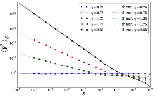
Figure 2: (Color online) The variance of the force on particles in a phase space cell due to particles in the corresponding stripe, plotted as a function of $\varepsilon$, for the different values of $\gamma$. The crosses indicate the points obtained from the numerical simulation described in the text and dotted lines are the corresponding analytical results, Eq. (56). We use units in which $\lambda_{x}=1$ and $g=1$.

Shown in Fig. 2 are the results of these numerical simulations compared with the theoretical results, Eq. (56), for a range of values of $\varepsilon$ and different values of $\gamma$. The agreement is excellent in all cases. Further we have verified that, except in the region where $\varepsilon$ approaches $\lambda_{x}$, the results are in excellent agreement with the expression (57) for the small $\varepsilon/\lambda_{x}$ behaviour. Thus we find results completely in line with our determination of the scalings in this limit for the $d$-dimensional case, leading to the different behaviours described in Section IV: for $\gamma=0.25$, in the range $\gamma<d/2$, the force fluctuations are independent of $\varepsilon$; for $\gamma=0.75$ and $\gamma=1.25$, in the range $d/2<\gamma<d/2+1$, the divergent 2-body term $\sim\varepsilon^{1-2\gamma}$ dominates at small $\varepsilon$, but is then overtaken at larger $\varepsilon$ by the flat behaviour of the the dominant $\varepsilon$-independent term in the 3-body term; for $\gamma=1.75$ and $\gamma=2.5$, both in the range $d/2+1<\gamma$ we have again at the smallest $\epsilon$ the behaviour $\sim\varepsilon^{1-2\gamma}$ from the 2-body term, but at larger $\epsilon$ instead the dominant behaviour $\varepsilon$-dependent term $\sim\varepsilon^{3-2\gamma}$ from the 3-body term.

VI Discussion and conclusions

Let us now discuss further the physical significance of these results, and in particular how they justify the basic qualitative distinction between interactions as we have anticipated in the introduction. We have considered a generic $N$-particle system with Hamiltonian dynamics described by a two body interaction with a pair force $\sim 1/r^{\gamma}$ and regularized below a scale $\varepsilon$ to a constant value. Introducing a coarse-graining in phase space, one obtains an equation for the coarse-grained phase space density with terms corresponding to the Vlasov equation, in addition to “non-Vlasov” terms which are functionals of the microscopic phase density. We then made the hypothesis that the typical amplitude of these terms can be estimated by assuming this microscopic phase space density to be given by a realization of an inhomogeneous Poissonian point process, in which the mean density is specified by the coarse-grained phase space density but the density fluctuations are uncorrelated. In other words we neglect all contributions due to correlation of density fluctuations with respect to the ones due to the simple products of mean densities. Doing so we have determined the scalings of these latter terms as a function of the different scales in the problem, of $\gamma$ and of the spatial dimension $d$. If the assumed hypothesis is valid (for large $N$), a limit in which the Vlasov equation applies is simply any one in which the derived non-Vlasov terms go to zero while the Vlasov terms tend to fixed finite values. Our results show firstly that, for any interaction in the class we have considered, such a limit exists and can be defined in different ways: notably, by taking $N$ to infinity at fixed values of the other scales, and in particular at fixed smoothing; or, alternatively, by taking the limit in which the coarse-graining scale, while always remaining small compared to the system size, is taken arbitrarily large compared to the other scales, and in particular the smoothing scale $\varepsilon$. However, when this limit is taken, there is a important difference between the case in which $\gamma>d$ or $\gamma<d$: for the former case the dominant correction term to the Vlasov limit is always strongly dependent on $\varepsilon$, while in the latter case the dominant term, at fixed $\lambda_{x}$, is independent of $\varepsilon$ in a wide range whose lower limit vanishes as $\lambda_{x}$ diverges. This different leading dependence on $\varepsilon$ corresponds to fluctuations which are sourced by quite different contributions in the two cases: for $\gamma>d$, the dominant fluctuation in the force on a coarse-graining cell comes from the contributions coming from forces on individual particles due to single particles which are “closeby”, i.e., within a radius $\varepsilon$: for $\gamma<d$, on the other hand, the dominant fluctuation comes from the coherent effect on two different particles in the cell coming from a single particle which is “far-away”, i.e. at a distance of order the size of the coarse-graining cell, or, even for $\gamma<d/2$, of order the size of the system. Given that these amplitudes are those of the terms describing the corrections to the Vlasov evolution due to the large, but finite, number of particles in a real system, this means that the dynamics of the particle system at a coarse-grained scale in the two cases is dominated by completely different contributions: by the particle distribution at the smallest scales when $\gamma>d$, and by the particle distribution at the coarse-graining scale or larger when $\gamma<d$. Thus in the latter case we can decouple the dynamics at the coarse-graining scale from that at smaller scales (the interparticle distance, the scale of particle size), while for $\gamma>d$ we cannot do so. Or, in the language of renormalisation theory, the former admit a kind of universality in which the coarse-grained dynamics is insensitive to the form of the interaction below this scale, while the latter do not. This is a basic qualitative distinction between the dynamics in these two cases, which corresponds naturally to what one call “short-range” or “long-range”. In order to distinguish it from the canonical distinction based on thermodynamical considerations, following (Gabrielli2010, ), we can refer to $\gamma>d$ as dynamically short-range, and $\gamma<d$ as dynamically long-range .

For what concerns quasi-stationary states the implications of this result and relevance of the classification are simple: for all cases one would expect that such states may exist (since the Vlasov limit exists) but the conditions for their existence, which requires that the time scales of their persistence be long compared to the system dynamical time, will be very different. For $\gamma>d$, their lifetime, which would be expected to be directly related to the amplitude of the non-Vlasov term, can be long only if the smoothing scale in the force is sufficiently large; in the case $\gamma<d$, their lifetime will be expected to be independent of $\varepsilon$. We note that this is precisely in line with results of analytical calculations based on the Chandrasekhar approach to estimation of the relaxation rate, and the results of numerical simulations of systems of this kind reported in (Gabrielli2010a, ).

These results are all, as we have emphasized, built on our central hypothesis that correlation of density fluctuations, associated with the finite particle number, may be neglected. To formulate it we must define a smooth mean phase space density by introducing a coarse-graining scale, which is assumed to be a “mesoscopic scale”: arbitrarily small compared to the system size, and yet large enough so that the phase space cell contains many particles. Our central hypothesis is not one of which we have proven the validity, but it is a consistent, simple and physically reasonable one, analogous to that of “molecular chaos” in the derivation of the Boltzmann equation. It is also in line with the fact that when the Vlasov approximation is valid, the system dynamics is defined in terms only of the mean density and fluctuations due to higher order density correlations are considered subdominant. We note above all that it leads to conclusions and behaviours which are very reasonable physically, even in the cases we have not focussed on but to which our analysis can be applied. For example, if we consider a hard repulsive core interaction without a smoothing, i.e. let $\varepsilon\rightarrow 0$ for $\gamma$ large, we infer that the force fluctuation on a coarse-grained cell diverges and that there is thus no Vlasov limit. Indeed in this case an appropriate two body collision operator is required to take into account the effects of interactions between particles.

Finally we note that the ensemble we have assumed to describe the fine-grained phase space density is a realization of a Poisson process with mean density given by the coarse-grained space. This implies that we include (Poissonian) fluctuations of particle number at all scales: indeed these (finite particle number) fluctuations are the source of the fluctuation terms in the dynamical equations which we have analysed. One could consider that it might be more appropriate physically to take, in estimating the fluctuations induced at a given coarse-grained density, the ensemble in which the particle number is constrained to be fixed in all coarse-graining cells. In other words we could average, given a coarse-grained phase space density, only over the configurations in which the particles, of fixed number in each cell, are distributed randomly within the cells. It is straightforward to verify, with the appropriate modification of the average, that doing so can only change our results for what concerns the large scale contributions to the force fluctuations: the diverging behaviours at small scales we have focussed on arise from the fact that there is a finite probability for a particle to be arbitrarily close to another one, and the local value of the density will at most modify the amplitude but not the parametric dependence of this term. On the other hand, our determinations of the parametric dependence of the contributions to the force fluctuations from the bulk will be expected to depend on how the particle fluctuations at larger scales are constrained .

In future work we plan to explore the possibility of developing the approach used in this article to understand and describe further the effect of the “non-Vlasov” — collisional — terms on the evolution of a finite $N$ system, i.e., to use it to develop a kinetic theory for the $N$ particle system. In this context it would be interesting to determine whether existing kinetic equations such as that of Lenard-Balescu, or variants of it developed in the literature (see, e.g., (Chavanis2012a, ; Chavanis2013, ) for a discussion and references), could be derived in a different way from this starting point, or even potentially modified or formulated differently. In this respect we note that the results derived here already provide a better basis for many derivations of such equations (and in particular the Lenard-Balescu equation) which take as a starting point the assumption that the Vlasov equation applies in the large $N$ limit (and then derive the kinetic equation for perturbations about it). It would be interesting also to clarify in particular the relation between this approach and that of Chandrasekhar which, as we have noted, when extended to a generic interaction has been shown Gabrielli2010a to give very consistent conclusions about the sensitivity of collisional relaxation of quasi-stationary states to the small scale regularisation. Likewise it would be interesting to try to test directly in numerical simulations for the validity of our central hypothesis about correlations, and also characterize using analytical methods the robustness of our central conclusions to the existence of different weak correlations of the density fluctuations.

We thank Bruno Marcos and Pascal Viot for very useful discussions.

References

- (1) A. Campa, T. Dauxois, and S. Ruffo, Phys. Rep. 480, 57 (2009)
- (2) T. Dauxois, S. Ruffo, E. Arimondo, and M. Wilkens, Lecture Notes in Physics Volume 602 (Springer Berlin / Heidelberg, 2002)
- (3) A. Campa, A. Giansanti, G. Morigi, and F. Sylos Labini, Dynamics and Thermodynamics of systems with long range interactions: theory and experiments, Vol. 970 (2008)
- (4) F. Bouchet, S. Gupta, and D. Mukamel, Physica A 389, 4389 (2010)
- (5) J. Binney and S. Tremaine, Galactic Dynamics, 2nd ed. (Princeton University Press, 2008)
- (6) F. Bouchet and J. Sommeria, J. Fluid Mech. 464, 165 (2002)
- (7) A. Olivetti, J. Barré, B. Marcos, F. Bouchet, and R. Kaiser, Phys. Rev. Lett. 103, 224301 (2009)
- (8) J. Sopik, C. Sire, and P.-H. Chavanis, Phys. Rev. E 72, 26105 (2005)
- (9) W. Braun and K. Hepp, Commun. Math. Phys. 113, 101 (1977)
- (10) H. Spohn, Large scale dynamics of interacting particles (Springer, 1991) ISBN 9783642843730
- (11) M. Hauray and P.-e. Jabin, Arch. Ration. Mech. Anal. 183, 489 (2007), arXiv:arXiv:1107.3821v5
- (12) S. Chandrasekhar, Astrophys. Journal. 97, 255 (1943)
- (13) M. Henon, Ann. d’Astrophysique 21, 186 (1958)
- (14) P.-H. Chavanis, J. Stat. Mech. Theory Exp. 2010, P05019 (2010)
- (15) R. T. Farouki and E. E. Salpeter, Astrophys. J. 427, 676 (1994)
- (16) R. T. Farouki and E. E. Salpeter, Astrophys. J. 253, 512 (1982)
- (17) P. H. Chavanis, Eur. Phys. J. Plus 127, 19 (Feb. 2012)
- (18) R. Balescu, Equilibrium and Non-Equilibrium Statistical Mechanics, Wiley-Interscience publication (John Wiley & Sons, 1975) ISBN 9780471046004
- (19) I. U. L. Klimontovich, The Statistical Theory of Non-equilibrium Processes in Plasma, International series of monographs in natural philosophy (M.I.T. Press, 1967)
- (20) D. R. Nicholson, Introduction to plasma theory (Cambridge Univ Press, 1983)
- (21) P.-H. Chavanis, Eur. Phys. J. Plus 128, 106 (2013)
- (22) T. R. Filho, M. Amato, and A. Figueiredo, Phys. Rev. E 89, 1 (2012), arXiv:1203.0082v1
- (23) T. Buchert and A. Domínguez, A&A 460, 443 (2005)
- (24) A. Gabrielli, M. Joyce, B. Marcos, and F. Sicard, J. Stat. Phys. 141, 970 (2010)
- (25) A. Gabrielli, M. Joyce, and B. Marcos, Phys. Rev. Lett. 105, 210602 (2010)
- (26) A. Gabrielli, F. Labini, M. Joyce, and L. Pietronero, Statistical Physics for Cosmic Structures (Springer, 2006) ISBN 9783540269991
- (27) A. Gabrielli and M. Joyce, Phys. Rev. E 81, 21102 (2010)