Evaluation of Constant Potential Method in Simulating Electric Double-Layer Capacitors

Abstract

A major challenge in the molecular simulation of electric double layer capacitors (EDLCs) is the choice of an appropriate model for the electrode. Typically, in such simulations the electrode surface is modeled using a uniform fixed charge on each of the electrode atoms, which ignores the electrode response to local charge fluctuations in the electrolyte solution. In this work, we evaluate and compare this Fixed Charge Method (FCM) with the more realistic Constant Potential Method (CPM), [Reed, et al., J. Chem. Phys., 126, 084704 (2007)], in which the electrode charges fluctuate in order to maintain constant electric potential in each electrode. For this comparison, we utilize a simplified LiClO4-acetonitrile/graphite EDLC. At low potential difference ($\Delta\Psi\leq$$2\text{\,}\mathrm{V}$), the two methods yield essentially identical results for ion and solvent density profiles; however, significant differences appear at higher $\Delta\Psi$. At $\Delta\Psi\geq$4\text{\,}\mathrm{V}$$, the CPM ion density profiles show significant enhancement (over FCM) of “inner-sphere adsorbed” Li+ ions very close to the electrode surface. The ability of the CPM electrode to respond to local charge fluctuations in the electrolyte is seen to significantly lower the energy (and barrier) for the approach of Li+ ions to the electrode surface.

I Introduction

Electric double-layer capacitors (EDLCs) are non-Faradaic, high power-density devices that have wide application in energy storage. Together with pseudo-capacitors, EDLCs make up a class of energy storage devices called super capacitors. The energy storage and release mechanism in EDLCs is rapid and possesses a long cycle life due to the physical nature of the charging/discharging process - in the charging process, ions in the electrolyte solution aggregate at the interface to form an electric double layer, which in turn induces charges on the electrode surfaces. Over the past decade, accompanying the recent bloom of novel electrode (i.e. nanoporous material) and electrolyte materials (i.e. ionic liquid), EDLCs have been the subject of numerous experimental studies.Choi et al. (2012); Aravindan et al. (2014) From these studies, the performance of EDLCs is affected by a number of different factors including, but not limited to, electrolyte compositionSato, Masuda, and Takagi (2004); Yuyama et al. (2006), interface structureWei et al. (2014); Ji et al. (2014) and surface area.Largeot et al. (2008); Itoi et al. (2011) As a result of these efforts, the performance of EDLCs have been significantly enhanced, extending their applicability.

These experimental studies have been complemented by a number of theoretical/computational studies ranging from atomistic simulation to mesoscale continuum modeling.Fedorov and Kornyshev (2014) Analytical continuum models have been developed to describe the electrode/electrolyte interface, for example, the Gouy-Chapman-Stern model.Wang and Pilon (2012); Wang, Thiele, and Pilon (2013) Classical Density Functional Theories (cDFT)Jiang and Wu (2013) have also been applied to estimate properties of EDLCs, which are more accurate than continuum models but considerably less computationally demanding than atomistic simulation. Atomistic simulations, however, have an advantage over the continuum models and cDFT because they provide a molecular-level description of the structure, dynamics and thermodynamics of EDLCs. Molecular simulation tools, such as ab-initio molecular dynamics (AIMD) simulation Ando, Gohda, and Tsuneyuki (2013) and classical molecular-dynamics (MD) simulation are widely used to investigate EDLC interfacial phenomena at the molecular level.

In molecular simulations of EDLCs, the modeling of the electrode is a particular challenge because of the difficulty in defining a consistent classical atomistic model for a conductor. In many MD studies of EDLCs, the electrode atoms are assumed to carry a uniform fixed charge. This Fixed Charge Method (FCM), however, neglects charge fluctuations on the electrode induced by local density fluctuations in the electrolyte solution.Yang et al. (2009, 2010); Shim, Kim, and Jung (2012); Feng and Cummings (2011); Feng et al. (2013) To explicitly take into account such fluctuations, the Constant Potential Method (CPM) was developed by Reed, et al.Reed, Lanning, and Madden (2007) This method is based on earlier work of Siepmann and Sprik Siepmann and Sprik (1995) in which the constraint of constant electrode potential was enforced on average using an extended Hamiltonian approach (similar to the Nosé methodNosé (1984) for constant temperature); however, in the CPM the constraint is applied instantaneously at every step. Additional corrections to the CPM were added later by Gingrich and Wilson.Gingrich and Wilson (2010) In the CPM, the electric potential $\Psi_{i}$ on each electrode atom is constrained at each simulation step to be equal to a preset applied external potential $V$, which is constant over a given electrode. This constraint leads to the following equation for the charge, $q_{i}$, on each electrode atom (where $i$ indexes the atoms in the electrode):

$$V=\Psi_{i}=\frac{\partial U}{\partial q_{i}}$$ (1)

where $U$ is the total Coulomb energy of the system.

The structure of the Coulomb energy expression is such that Eq. 1 is a system of linear equations for $q_{i}$ and can be solved with standard linear algebra techniques. To guarantee that the linear system corresponding to Eq. 1 has a solution, the electrode point charges are generally replaced with a narrow Gaussian charge distribution. For a detailed study of the optimal choice for Gaussian width, see GingrichGingrich (2010).

Several studies of EDLCs employing the CPM have been reported. Merlet, et al.Merlet et al. (2011, 2012); Merlet, Salanne, and Rotenberg (2012); Merlet et al. (2013a) studied a nanoporous carbon electrode in contact with electrolyte consisting of an ionic liquid or an ionic liquid/acetonitrile mixture. Vatamanu and coworkersVatamanu, Borodin, and Smith (2010); Vatamanu et al. (2012); Vatamanu, Borodin, and Smith (2012); Vatamanu et al. (2013) investigated ionic liquid electrolytes with carbon or gold electrodes using the smooth particle mesh Ewald (SMPE)Kawata and Mikami (2001); Kawata, Mikami, and Nagashima (2002) method to simplify the calculation. The hydration of metal-electrode surfaces was examined by Limmer, et al.Limmer et al. (2013a, b)

In all of these studies, detailed comparisons of the CPM with the fixed charge method have been lacking. In a recent paper, Merlet, et al. Merlet et al. (2013b) examined the differences between CPM and FCM simulations as measured by the relaxation kinetics in EDLC with nanoporous carbide-derived carbon electrode and the electrolyte structure at interface in EDLC with planar graphite electrode.It was showed that CPM predicts more reasonable relaxation time than FCM. For the electrolyte structure, this study showed that there are some quantitative differences between the results of the two methods, but the qualitative features were unchanged for these ionic-liquid based EDLCs.

In this work, we study an organic electrolyte/salt-based ELDC, namely an LiClO4/acetonitrile electrolyte at a graphite electrode. To compare the results for this system using the CPM and FCM, several structural aspects normally reported in EDLC simulations are studied for comparison, specifically, the particle and charge density profiles near the electrodes and the solvation structure of the cation (Li+) both in bulk and near the surface.

II Models and Methodology

In our simulations, the atoms of the electrolyte solution are placed between two carbon electrodes, each consisting of three graphite layers. The simulation geometry is shown in Fig. 1, which shows a snapshot from a simulation at 298K with a potential difference, $\Delta\Psi$ of $2\text{\,}\mathrm{V}$. For the production runs, the distance between the two inner-most electrode layers (labeled L1 and R1, respectively, in Fig. 1) is $6.365\text{\,}\mathrm{n}\mathrm{m}$, which is far beyond the Debye length ($0.2\text{\,}\mathrm{n}\mathrm{m}$). The electrolyte between the electrodes consists of 588 acetonitrile molecules and 32 Li+/ClO4- pairs, corresponding to a LiClO₄ concentration of $1.00\text{\,}\mathrm{M}$. The total dimensions of the cell are 2.951, 2.982 and $8.040\text{\,}\mathrm{n}\mathrm{m}$. The positions of the electrode carbon atoms are held fixed during the simulation.

To model the molecular interactions we employ a variety of literature force fields. For acetonitrile, we use the united atom model of Edwards, et al.Edwards, Madden, and McDonald (1984) For the ions, we use the forcefield of Eilmes and Kubisiak,Eilmes and Kubisiak (2011) excluding the polarizability terms. The interaction parameters for the graphite electrode carbon atoms are taken from Ref. Cole and Klein, 1983. Lorentz-Berthelot mixing rules are used to construct all cross interactions.

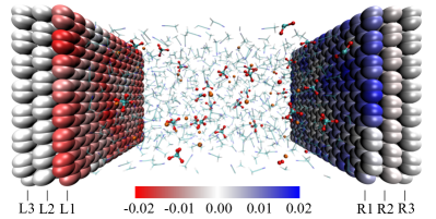
Figure 1: Simulation snapshot at 298K with $\Delta\Psi=2$V: negative electrode is on left and positive is on right. The color of each electrode atom indicates its charge (refer to color scale bar, unit e). The electrolyte solution is shown between the two electrodes. Orange spheres: Li+, Red spheres: O in ClO4-, cyan spheres: Cl in ClO4-, transparent stick models: acetonitrile. For clarity, in this figure, the distance between L1 and R1 ($5.43\text{\,}\mathrm{n}\mathrm{m}$) is smaller than that used in the production runs.

In this slab geometry, we define the z-axis as the direction normal to the electrodes and apply periodic boundary conditions only in the x-y plane (parallel to the graphite layers). Unlike the original CPM, which used 2d-periodic Ewald sums,De Leeuw and Perram (1979); Kawata and Mikami (2001) 3d-periodic Ewald sums with shape correctionsYeh and Berkowitz (1999) were used in this work to improve the calculation speed, with a volume factor set to 3. The correction term to the usual 3d-periodic energy expression is given by (see Eq. A.21 in Ref. Gingrich, 2010):

$$\frac{2\pi}{V}\left(\sum_{i}q_{i}z_{i}\right)^{2}$$ (2)

In studies using FCM, either the uniform charge on each electrode atom is either arbitrarily chosenYang et al. (2010); Shim, Kim, and Jung (2012); Feng et al. (2013) or is estimated using a time-consuming trial and error procedure to yield the specified electric potential difference,Feng and Cummings (2011) which is calculated by numerically integrating the Poisson equation using the charge density profile. The CPM is able to predict the explicit average charge on each electrode atom at a given potential difference; therefore, for consistency, in our FCM simulations we set the charge on each electrode atom to the average charge per atom obtained by the CPM calculations at the same potential difference. Otherwise, all other force-field parameters in the FCM simulations are identical to those used in the CPM simulations.

All simulations were performed using the molecular-dynamics simulation code LAMMPS,Plimpton (1995) modified to implement the CPM, using a time step of $1\text{\,}\mathrm{f}\mathrm{s}$. Constant $NVT$ conditions are enforced using a Nosé-Hoover thermostat with a relaxation time of 100 fs and a temperature of $298\text{\,}\mathrm{K}$. The cutoffs for all non-bonded interactions are $1.4\text{\,}\mathrm{n}\mathrm{m}$. For the Ewald sums, an accuracy (relative RMS error in per-atom forces) is set to $10^{-8}$. The parameter of the Gaussian electrode charge distribution (see Eq. S2 in supplementary material) is set to $19.79\text{\,}\mathrm{n}\mathrm{m}^{-1}$, which is the same as in Ref. Reed, Lanning, and Madden, 2007. All results reported here are statistical averages taken from runs of 25 to $30\text{\,}\mathrm{n}\mathrm{s}$ in length, each preceded by $2\text{\,}\mathrm{n}\mathrm{s}$ of equilibration. Further details as to the CPM method and our implementation in LAMMPS can be found in the supplementary material.

III Results and discussion

III.1 Electrode charge distribution

Unlike the FCM, the CPM allows the individual atom charges on the electrode to fluctuate in response to local charge rearrangements in the electrolyte. The total charges on each layer for several potential differences are shown in Table 2. The net electrode charge for each simulation does not show values statistically significant from zero, as expected. In a perfect conductor, the charges on the electrode atoms would be concentrated entirely on the electrode surface layers (L1 and R1 in Fig. 1); however, in the CPM the charge distribution on the electrode is approximated by discrete point charges centered on the electrode itself, so a small amount of charge is found on the second layer and to a much lesser extent the third.

Table 1: Average total charge on each electrode layer

Layer	$0\text{\,}\mathrm{V}$	$2\text{\,}\mathrm{V}$	$4\text{\,}\mathrm{V}$	$5\text{\,}\mathrm{V}$
L3	$0.00(2)$	$0.03(2)$	$0.06(2)$	$0.06(2)$
L2	$0.02(5)$	$0.33(5)$	$0.64(4)$	$0.75(5)$
L1	$-0.1(4)$	$-3.4(4)$	$-6.6(4)$	$-8.4(5)$
R1	$0.0(4)$	$3.3(4)$	$6.5(4)$	$8.4(5)$
R2	$0.01(5)$	$-0.29(4)$	$-0.58(5)$	$-0.75(6)$
R3	$0.00(2)$	$-0.02(2)$	$-0.03(2)$	$-0.06(2)$
Total	$0.01(6)$	$0.02(6)$	$0.04(6)$	$0.01(6)$

Figure 2 is a log-linear plot of the probability distribution of individual electrode atom charges, $p(q)$, on the inner electrode layers for various potential differences. For the inner layer of the positively charged electrode (R1), the charge distribution is well described by a Gaussian distribution over the entire range of potential differences studied ($\Delta\Psi$ = $0\text{\,}\mathrm{V}$ to $5\text{\,}\mathrm{V}$). For the negatively charged electrode (L1), this is true at the lower potential differences (up to $\Delta\Psi$ = $2\text{\,}\mathrm{V}$), but the charge distribution takes on a bimodal structure at higher potential differences ($\Delta\Psi$ = $4\text{\,}\mathrm{V}$ and $5\text{\,}\mathrm{V}$). A similar non-Gaussian charge distribution has also been seen in simulations at the negative electrode of a H2O/Pt system;Limmer et al. (2013a) however, that system differs somewhat from our simulated system in that no ions are present. The bimodal charge distribution at the higher potential differences in this system highlights an important difference between the CPM and the FCM. Unlike the FCM, the electrode charges in the CPM can adjust to respond to local fluctuations in the electrolyte/ion charge density. As we will see in the next section, this second peak in $p(q)$ seen at high potential differences is due to the presence of Li+ ions near the electrode surface, which induce higher than average local charges on the adjacent electrode.

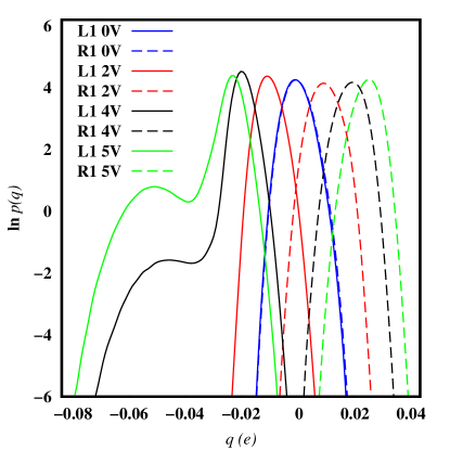
Figure 2: Distribution of electrode atom charges for the inner electrode layers at various potential differences: L1 (solid lines) and R1(dashed lines).

III.2 Density profiles for ions and electrolytes

To better understand the origin of the bimodal charge distributions in the CPM at high potential difference, we examine the ion density profiles at the interface and compare the results obtained using CPM and FCM (Fig. 3).

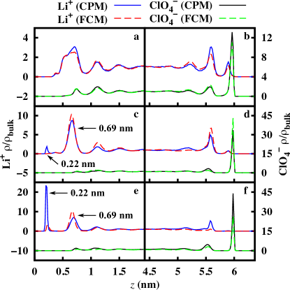
Figure 3: Ion densities near each of the two electrodes (L1 and R1) for various applied potential differences (a) L1; $\Delta\Psi=$2\text{\,}\mathrm{V}$$, (b) R1; $\Delta\Psi=$2\text{\,}\mathrm{V}$$, (c) L1; $\Delta\Psi=$4\text{\,}\mathrm{V}$$ (d) R1 $\Delta\Psi=$4\text{\,}\mathrm{V}$$ (e) L1; $\Delta\Psi=$5\text{\,}\mathrm{V}$$, (f) R1; $\Delta\Psi=$5\text{\,}\mathrm{V}$$. The negatively and positively charged electrodes (L1 and R1) are at $z=0$ and $6.365\text{\,}\mathrm{n}\mathrm{m}$, respectively.

At the lowest non-zero potential difference ($\Delta\Psi$ = $2\text{\,}\mathrm{V}$), the ion density profiles for the CPM and FCM methods show relatively minor quantitative differences in peak heights, but otherwise the density peak positions and overall structure are identical. At higher potential differences ($4\text{\,}\mathrm{V}$ and $5\text{\,}\mathrm{V}$), however, qualitative differences emerge. At $\Delta\Psi$ = $4\text{\,}\mathrm{V}$, a peak in the Li+ density profile near the negatively charged electrode (L1) at $0.22\text{\,}\mathrm{n}\mathrm{m}$ appears in the CPM calculation, but is absent in the FCM results. This peak represents inner-sphere adsorbed Li+ ions that no longer possess a full solvation shell of acetonitrile, but are also “partially solvated” by the electrode. The existence of these inner-sphere adsorbed ions is made possible because the CPM allows for more physically correct electrode charge distribution - one that can respond to the presence of the nearby Li+ ion with locally larger-than-average negative electrode charges. The partial desolvation was reported to be highly related with the confinement of ions, which fundamentally affects the capacitance.Merlet et al. (2013c)

As the potential difference is increased beyond $4\text{\,}\mathrm{V}$, the inner-sphere adsorbed ion peak grows substantially. For the FCM, we see this peak at $5\text{\,}\mathrm{V}$, but it has an amplitude that is much smaller than that predicted by the CPM. In addition, Fig. 3 also shows that the height of the Li+ density peak at $0.69\text{\,}\mathrm{n}\mathrm{m}$, representing the first fully solvated outer-sphere adsorbed Li+ layer in the ELDC, is overestimated at $\Delta\Psi=$ $4\text{\,}\mathrm{V}$ and $5\text{\,}\mathrm{V}$ in the FCM. This is due to the migration of Li+ ion density from the inner-spher adsorbed peak at $0.21\text{\,}\mathrm{n}\mathrm{m}$, compared with the CPM.

In contrast to Li+, the ClO4- density profiles are nearly identical for both methods at all studied potential differences. The charge density in ClO4- is spread out over a larger radius and does not create as large a local charge concentration in the electrolyte solution to perturb the electrode charge distribution enough to affect the density profiles.

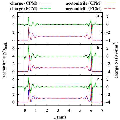
Figure 4: Acetonitirle density and charge profiles at various applied potentials (a) $\Delta\Psi=$2\text{\,}\mathrm{V}$$, (b) $\Delta\Psi=$4\text{\,}\mathrm{V}$$, (c) $\Delta\Psi=$5\text{\,}\mathrm{V}$$. Vertical lines show the position of the electrode inner layers L1 (left) and R1 (right).

In Fig. 4 we plot the solvent (acetonitrile, center of mass) and charge density profiles. Unlike the ion density profiles, the density profiles for acetonitrile are identical for both methods up to a potential difference of 4V. However, at $\Delta\Psi=$ 5V the acetonitrile peak closest to the negative electrode (L1) splits into two peaks in the CPM, a feature not seen in the FCM calculation. This is because the large amount of electrode solvated Li+ seen in the CPM pulls the acetonitrile molecules in its solvation shell closer to the surface.

The structure of the electric double layer in this system is best illustrated by the charge density profile (see Figure 4). For this quantity the results for both methods (CPM and FCM) are very similar with the only difference coming at high potential difference, where small charge peaks corresponding to the electrode-solvated Li+ are present in the CPM result, but not in the FCM.

III.3 Structure of inner-sphere adsorbed Li+

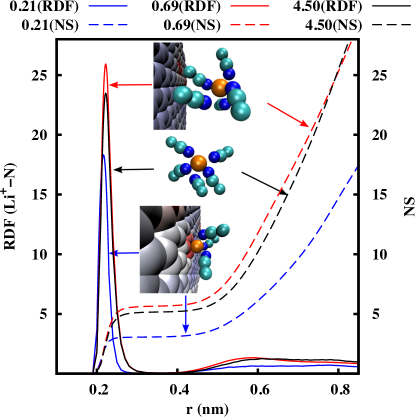
(a)

Figure 5: Radial distribution functions (RDF,solid lines) and corresponding number of solvent molecules (NS, dashed lines) between Li+ and N atom in acetonitrile for $\Delta\Psi$ = $4\text{\,}\mathrm{V}$. In the legend the number indicates the distance (nm) from the negative electrode surface to the center of bin (with width $\pm$$0.02\text{\,}\mathrm{n}\mathrm{m}$) containing the Li+ ion. The insets show typical snapshots of the Li+ solvation structure for each distance studied.

In this work, the principal difference between the results derived from the CPM and FCM is the appearance in the CPM of Li+ ions very close to the negatively charged electrode at high potentials. This inner-sphere adsorbed Li+ also is seen in the FCM, but only at very low concentration at the highest potential difference studied. To examine this feature more closely, we analyze the solvation structure of Li+ by plotting in Fig. 5 (for $\Delta\Psi=$4\text{\,}\mathrm{V}$$) the CPM radial distribution function (RDF) between the Li+ ion and the acetonitrile N for three Li+ distances from the electrode surface: 0.21, 0.69 and $4.50\text{\,}\mathrm{n}\mathrm{m}$. These correspond to the inner-sphere adsorbed Li+, the first layer of outer-sphere adsorbed Li+ and the bulk conditions, respectively. Also plotted in Fig. 5 are the number of solvent molecules (NS) within a given radius - for the bulk ions, the first plateau in this quantity corresponds to the equilibrium coordination number. The results of RDF and NS for the FCM or other potential differences are identical to that shown for the CPM at $4\text{\,}\mathrm{V}$ (Fig. 5) - except for the fact that no Li+ ions at $0.21\text{\,}\mathrm{n}\mathrm{m}$ for the CPM at $\Delta\Psi=$2\text{\,}\mathrm{V}$$ and for the FCM at $2\text{\,}\mathrm{V}$ and $4\text{\,}\mathrm{V}$ are detected and therefore no RDF (nor NS) data was obtained.

At $z$ = $0.69\text{\,}\mathrm{n}\mathrm{m}$ and $4.50\text{\,}\mathrm{n}\mathrm{m}$, the Li+ ion is fully solvated by the acetonitrile solvent and the first solvation shell peaks for both distances are nearly identical with a peak distance of $0.22\text{\,}\mathrm{n}\mathrm{m}$. In addition, the coordination number (given by the plateau value of NS) of each Li+ ion is equal to about 5.0 for the “bulk” case ($4.50\text{\,}\mathrm{n}\mathrm{m}$), just slightly smaller than that for the first fully solvated peak with 5.4, presumably due to the enhanced acetonitrile density near the electrode region (see Fig. 4). The value for the “bulk” is consistent with that seen in other simulation studies of bulk acetonitrile-lithium salt solutions.Oliveira Costa and López Cascales (2010); Spångberg and Hermansson (2004)

For Li+ ions at $0.21\text{\,}\mathrm{n}\mathrm{m}$ from the electrode, however, the solvent coordination is significantly reduced from the bulk value to 3.1 due to partial solvation by the electrode atoms themselves. The bottom inset in Fig. 5 shows a representative snapshot from the CPM simulation ($\Delta\Psi=$4\text{\,}\mathrm{V}$$) of an electrode-solvated ion and its nearby environment. In the CPM, because the charges on the electrode can fluctuate individually in response to the local electrolyte charge distribution, the presence of the Li+ ion very close to the electrode induces larger than average negative charges on the nearby electrode ions, as seen in the inset. The ability of the electrode to respond to local fluctuations is necessary for the stabilization of the electrode-solvated Li+ below $\Delta\Psi\lesssim$4\text{\,}\mathrm{V}$$, as no such ions are seen in the FCM simulations in this range. At $5\text{\,}\mathrm{V}$, such electrode-solvated ions are seen in the FCM, but at significantly lower concentration than in the CPM, indicating a much higher energy for such configurations in the FCM, relative to the CPM. We have confirmed that sampling in the simulations is sufficient, as we see multiple crossings and recrossings of Li+ ions between the positions at $0.69\text{\,}\mathrm{n}\mathrm{m}$ and $0.21\text{\,}\mathrm{n}\mathrm{m}$.

IV Summary

In this work, two methods, the Constant Potential Method (CPM) and the Fixed Charge Method (FCM), are compared in a simulation of a model for a LiClO4-acetonitrile/graphite electric double-layer capacitor. The major difference between the two methods is that in the CPM the charges on the individual electrode atoms can fluctuate in response to local fluctuations in electrolyte charge density, whereas those charges for the FCM are static. For this system, there are no measurable differences between the results of these two methods at low potential differences ($\Delta\Psi\leq$2\text{\,}\mathrm{V}$$); however, at larger potential differences significant qualitative differences emerge in the EDLC ion spatial distribution.

At a potential difference of 4V, a new peak in the Li+ density profile appears in the CPM calculation at 0.21 nm away from the electrode. This peak - absent in the FCM calculation - corresponds to a inner-sphere adsorbed Li+ ion that is close enough to the electrode to have lost some of its acetonitrile solvation shell and is partially solvated by the electrode atoms. For this electrode-solvated Li+ ion the acetonitrile coordination number is reduced from about 5.0 for a fully solvated ion to 3.1. This partial solvation is possible because in the CPM the electrode atom charges can respond to local fluctuations in the electrolyte charge density - in this case negative charges build up in the CPM electrode near the lithium ion. This ability lowers the energy of the “electrode-solvated” Li+ ion relative to that of a fixed-charge electrode (as in the FCM). This close approach of Li+ to the electrode is possible in the FCM, but only at higher electrode potential differences and a considerably lower concentrations than when CPM is used. The energetics of the approach of a Li+ ion to the electrode is important in many pseudo-capacitor applications, and, as our calculations show, the CPM would be preferable to the FCM in the calculation of the barrier energy of this process because it more accurately represents the fluctuating charges on the electrode.

^∗ Author to whom correspondence should be addressed

Table of Contents

• Details of Constant Potential Method

• Implementation of CPM in LAMMPS

S1 Constant Potential Method
In what follows, the charge and position vector of an electrode (electrolyte) atom are designated as $Q_{i}$ ($q_{j}$) and $\textbf{R}_{i}$ ($\textbf{r}_{j}$), respectively. Starting from Eq. 1 in the main text, the potential at the position of a selected electrode atom ($l$) with the charge as $Q_{l}$ and the positon as $\textbf{R}_{l}$ can be calculated by:

$$\Psi_{l}=\Psi_{l}^{\textrm{kspace}}+\Psi_{l}^{\textrm{real}}+\Psi_{l}^{\textrm{self}}+\Psi_{l}^{\textrm{slab}}$$ (S1)

Here $\Psi_{l}^{\textrm{kspace}}$ the $k$-space contribution from the 3-d Ewald sum; $\Psi_{l}^{\textrm{real}}$ is the corresponding real-space contribution; $\Psi_{l}^{\textrm{self}}$ is the self-correction and $\Psi_{l}^{\textrm{slab}}$ is the correction for the slab geometry. To guarantee the solvability of the CPM linear equations, Gaussian charges are used for electrode atomsGingrich (2010)

$$Q_{i}(\textbf{r})=Q_{i}\left(\frac{\eta^{2}}{\pi}\right)^{3/2}e^{-\eta^{2}\left(\textbf{r}-\textbf{R}_{i}\right)^{2}}$$ (S2)

Here $\eta$ is the parameter defining the width of the distribution.

Each portion of the potential for the mixed electrode (Gaussian charge) and electrolyte (point charge) system are obtained as follows.

Real-space contributions: The Ewald expression for the real-space contribution is

$$\Psi_{l}^{\textrm{real}}=\frac{1}{2}\sum_{i=1}^{n^{\prime}}Q_{i}\frac{\textrm{erfc}\left({\alpha}\,r_{li}\right)-\textrm{erfc}\left(\frac{\eta}{\sqrt{2}}r_{li}\right)}{r_{li}}+\sum_{j=1}^{m}q_{j}\frac{\textrm{erfc}\left({\alpha}\,r_{lj}\right)-\textrm{erfc}\left({\eta}\,r_{lj}\right)}{r_{lj}}$$ (S3)

Where $n^{\prime}$ denotes the $i=l$ term is excluded. $r_{li}=\lvert\textbf{R}_{l}-\textbf{R}_{i}\rvert$ and $r_{lj}=\lvert\textbf{R}_{l}-\textbf{r}_{j}\rvert$.

k-space contributions: The Ewald expression for the $k$-space contribution is

$$\Psi_{l}^{\textrm{kspace}}=\frac{1}{V}\sum_{\textbf{k}>0}\Gamma(\kappa)\left[e^{-i\,\textbf{k}{\cdot}\textbf{R}_{l}}S(\textbf{k})+e^{i\,\textbf{k}{\cdot}\textbf{R}_{l}}S(-\textbf{k})\right]$$ (S4)

Following the notation in Refs. Moore, ; Gingrich, 2010, here k is a reciprocal lattice vector, $\kappa=\lvert{\textbf{k}}\rvert$ and $\Gamma(\kappa)$ is the Fourier coefficient of the Gaussian function used in the Ewald sum

$$\Gamma(\kappa)=\frac{4{\pi}e^{-\kappa^{2}/4\alpha^{2}}}{\kappa^{2}}$$ (S5)

In Eq. S4, $S(\textbf{k})$ is the structure factor, given as

$$S(\textbf{k})=\sum_{i=1}^{n}Q_{i}e^{i\,\textbf{k}{\cdot}\textbf{R}_{i}}+\sum_{j=1}^{m}q_{j}e^{i\,\textbf{k}{\cdot}\textbf{r}_{j}}$$ (S6)

Self correction:

$$\Psi_{l}^{\textrm{self}}=\frac{\sqrt{2}\eta-2\alpha}{\sqrt{\pi}}Q_{l}$$ (S7)

Slab correction:

$$\Psi_{l}^{\textrm{slab}}=\frac{4\pi Z_{l}}{V}\left(\sum_{i=1}^{n}Q_{i}Z_{i}+\sum_{j=1}^{m}q_{j}z_{j}\right)$$ (S8)

where $Z_{i}$ is the $z$ component electrode atom position and $z_{j}$ is the corresponding quantity for an electrolyte atom.

The potential expression can then be rewritten as

$$\Psi_{l}=\sum_{i}^{n}a_{li}Q_{i}+\sum_{j}^{m}b_{lj}q_{j}$$ (S9)

where $a_{li}$ is a function of the position of selected electrode atom ($\textbf{R}_{l}$) and that of other electrode atoms ($\textbf{R}_{i}$) only, which are constant because all electrode atoms are fixed. In opposite, $\textbf{r}_{j}$ is varying during the simulation and thus ${b_{lj}}$ is updated every timestep. Because $\Psi_{l}$ is equal to the external potential $V$, above equation becomes

$$\sum_{i}^{n}a_{li}Q_{i}=V-\sum_{j}^{m}b_{lj}q_{j}$$ (S10)

Similarly we can obtain a linear equation for each electrode atom. With $\textbf{Q}=[Q_{1},Q_{2},\cdots,Q_{n}]$ as unknown, the linear system can be then written as

$$\textbf{A}\textbf{Q}=\textbf{V}-\textbf{B}$$ (S11)

By solving this well-determined linear equations system the explicit charge for electrode atoms can be determined.

S2 Implementation in LAMMPS

The implemented code includes three functions: setting up the linear system of equations, solving the linear system and updating atom charges, energy and per-atom forces. The code can be downloaded through https://code.google.com/p/lammps-conp/

Determining the real-space contribution to A and B is similar to the real-space Coulombic energy calculation in LAMMPS, but without using the table technique (see the table keyword in pair_modify command in the LAMMPS manual for details). The self correction and slab correction portion are straightforward and the approach is similar to that of the corresponding components of the energy calculation in LAMMPS. However the Ewald sum contribution is obtained in a different way. Elements in A depend on the positions of electrode atoms only, which is constant during the simulation (assuming fixed electrode atoms). Therefore, at the initial stage, all MPI tasks collect the coordinates of all electrode atoms and calculate Ewald sum contribution to A individually. In contrast, B is only the summation of the contribution from only electrolyte atoms, so that Ewald sum portion in B is calculated in a similar way as the Ewald sum in group/group interaction calculation in LAMMPS, which each MPI task only calculates the portion in its atom list and then sum them together.

At the initial stage, the matrix inverse of A is obtained using LAPACK. In each step, at the second half step of the velocity-Verlet, the B is calculated and the charges of electrode atoms obtained, after which the additional energy and per-atom force are calculated (See reference Gingrich, 2010 for details of the additional terms) and added to original energy and per-atom force.

References

- Gingrich (2010) T. Gingrich, Simulating Surface Charge Effects in Carbon Nanotube Templated Ionic Crystal Growth, Ph.D. thesis, University of Oxford (2010).
- (2) S. G. Moore, “Calculating Per-Atom and Group/Group Quantities Using the Lattice Sum Method,” http://lammps.sandia.gov/doc/PDF/kspace.pdf.