Estimating Maximally Probable Constrained Relations by Mathematical Programming

Abstract

Estimating a constrained relation is a fundamental problem in machine learning. Special cases are classification (the problem of estimating a map from a set of to-be-classified elements to a set of labels), clustering (the problem of estimating an equivalence relation on a set) and ranking (the problem of estimating a linear order on a set). We contribute a family of probability measures on the set of all relations between two finite, non-empty sets, which offers a joint abstraction of multi-label classification, correlation clustering and ranking by linear ordering. Estimating (learning) a maximally probable measure, given (a training set of) related and unrelated pairs, is a convex optimization problem. Estimating (inferring) a maximally probable relation, given a measure, is a $01$-linear program. It is solved in linear time for maps. It is NP-hard for equivalence relations and linear orders. Practical solutions for all three cases are shown in experiments with real data. Finally, estimating a maximally probable measure and relation jointly is posed as a mixed-integer nonlinear program. This formulation suggests a mathematical programming approach to semi-supervised learning.

1 Introduction

Given finite, non-empty sets, $A$ and $B$, equal or unequal, the problem of estimating a relation between $A$ and $B$ is to decide, for every $a\in A$ and every $b\in B$, whether or not the pair $ab$ is related. Classification, for instance, is the problem of estimating a map from a set $A$ of to-be-classified elements to a set $B$ of labels by choosing, for every $a\in A$, precisely one label $b\in B$. Clustering is the problem of estimating an equivalence relation on a set $A$ by deciding, for every $a,a^{\prime}\in A$, whether or not $a$ and $a^{\prime}$ are in the same cluster. Ranking is the problem of estimating a linear order on a set $A$ by deciding, for every $a,a^{\prime}\in A$, whether or not $a$ is less than or equal to $a^{\prime}$. In none of these three examples are the decisions pairwise independent: If the label of $a\in A$ is $b\in B$, it cannot be $b^{\prime}\in B\setminus\{b\}$. If $a$ and $a^{\prime}$ are in the same cluster, and $a^{\prime}$ and $a^{\prime\prime}$ are in the same cluster, $a$ and $a^{\prime\prime}$ cannot be in distinct clusters. If $a$ is less than $a^{\prime}$, $a^{\prime}$ cannot be less than $a$, etc. Constraining the set of feasible relations to maps, equivalence relations and linear orders, resp., introduces dependencies.

We define a family of probability measures on the set of all relations between two finite, non-empty sets such that the relatedness of any pair $ab$ and the relatedness of any pair $a^{\prime}b^{\prime}\not=ab$ are independent, albeit with the possibility of being conditionally dependent, given a constrained set of feasible relations. With respect to this family of probability measures, we study the problem of estimating (learning) a maximally probable measure, given (a training set of) related and unrelated pairs, as well as the problem of estimating (inferring) a maximally probable relation, given a measure. Solutions for classification, clustering and ranking are shown in experiments with real data. Finally, we state the problem of estimating the measure and relation jointly, for any constrained set of feasible relations, as a mixed-integer nonlinear programming problem (MINLP). This formulation suggests a mathematical programming approach to semi-supervised learning. Proofs are deferred to Appendix A.

2 Related Work

(a)

(b)

Figure 1: Bayesian models of probability measures. a) The model of probability measures on binary relations we consider, in plate notation. b) A more general model of probability measures on subsets.

Estimating a constrained relation is a special case of structured output prediction [1], the problem of estimating, for a set $S$ and a set $z\subseteq 2^{S}$ of feasible subsets of $S$, from observed data $x$, one feasible subset $y\in z$ of $S$ so as to maximize a margin, as in [2], entropy, as in [3], or a conditional probability of $y$, given $x$ and $z$, as in this work. For relations, $S=A\times B$ with $A\not=\emptyset$ and $B\not=\emptyset$.

The Bayesian model of probability measures on the set of all relations between two sets we consider (Fig. 1) is more specific than the general Bayesian model for structured output prediction (Fig. 1). Firstly, we assume that the relatedness of a pair $ab$ depends only on one observation, $x_{ab}$, associated with the pair $ab$. We consider no observations associated with multiple pairs. Secondly, we assume that the relatedness of any pair $ab$ and the relatedness of any pair $a^{\prime}b^{\prime}\not=ab$ are independent, albeit with the possibility of being conditionally dependent, given a constrained set $z$ of feasible relations.

One probabilistically principled way of estimating a constrained subset (such as a relation) from observed data is by maximizing entropy [3]. The maximum probability estimation we perform is different. It is invariant under transformations of the probability measure that preserve the optimum (possibly a disadvantage), and it does not require sampling.

The problem of estimating a maximally probable equivalence relation with respect to the probability measure we consider is known in discrete mathematics as the Set Partition Problem [4] and in machine learning as correlation clustering [5, 6]. The state of the art in solving this NP-hard problem is by branch-and-cut, exploiting properties of the Set Partition Polytope [7]. Correlation clustering differs from clustering based on (non-negative) distances. In correlation clustering, all partitions are, a priori, equally probable. In distance-based clustering, the prior probability of partitions is typically different from the equipartition (otherwise, the trivial solution of one-elementary clusters would be optimal). Parameter learning for distance-based clustering is discussed comprehensively in [8]. We discuss parameter learning for equivalence relations and thus, correlation clustering. Closely related to equivalence relations are multicuts [4]; for a complete graph, the complements of the multicuts are the equivalence relations on the node set. Multicuts are used, for instance, in image segmentation [9, 10, 11, 12]. The probability measure on a set of multicuts defined in [10] is a special case of the probability measure we discuss here.

The problem of estimating a maximally probable linear order with respect to the probability measure we consider is known as the Linear Ordering Problem. The state of the art in solving this NP-hard problem is by branch-and-cut, exploiting properties of the Linear Ordering Polytope. The problem and polytope are discussed comprehensively in [13], along with exact algorithms, approximations and heuristics. Solutions of the Linear Ordering problem are of interest in machine learning, for instance, to predict the order of words in sentences [14]. Our experiments in Section 6.3 are inspired by the experiments in [14]. Unlike in [14], we do not use any linguistic features and assess solutions of the Linear Ordering Problem explicitly.

We concentrate on feature vectors in $\{0,1\}^{K}$, for a finite index set $K$. This is w.l.o.g. on a finite state computer and has the advantage that every probability measure on the feature space has a (unique) multi-linear polynomial form [15]. We approximate this form by randomized multi-linear polynomial lifting, building on the approximation of polynomial kernels proposed in [16]. This modeling of probability measures by linear approximations of multi-linear polynomial forms is in stark contrast to the families of nonlinear, nonconvex functions modeled by (deep) neural networks.

3 Probability Measures on a Set of Binary Relations

For any finite, non-empty sets, $A$ and $B$, equal or unequal, we define the probability of any relation $y^{\prime}\in 2^{A\times B}$ between these sets with respect to (i) a set $z^{\prime}\subseteq 2^{A\times B}$ called the set of feasible relations (ii) a finite index set $J$ and, for every $ab\in A\times B$, an $x_{ab}\in\{0,1\}^{J}$ called the feature vector of the pair $ab$ (iii) a finite index set $K$ and a $\theta\in\mathbb{R}^{K}$ called a parameter vector. The probability measure is defined with respect to a Bayesian model in four random variables, $X$, $Y$, $Z$, and $\Theta$. The model is depicted in Fig. 1. The random variables and conditional probability measures are defined below.

• For any $ab\in A\times B$, a realization of the random variable $X_{ab}$ is a (feature) vector $x_{ab}\in\{0,1\}^{J}$. Thus, a realization of the random variable $X$ is a map $x:A\times B\to\{0,1\}^{J}$ from pairs $ab$ to their respective feature vector $x_{ab}$.

• For any $ab\in A\times B$, a realization of the random variable $Y_{ab}$ is a $y_{ab}\in\{0,1\}$. Hence, a realization of the random variable $Y$ is the characteristic vector $y\in\{0,1\}^{A\times B}$ of a relation between $A$ and $B$, namely the relation $y^{\prime}:=\{ab\in A\times B\ |\ y_{ab}=1\}$.

• A realization of the random variable $Z$ is a set $z\subseteq\{0,1\}^{A\times B}$ of characteristic vectors. It defines a set $z^{\prime}\subseteq 2^{A\times B}$ of feasible relations, namely those relations $y^{\prime}$ whose characteristic vector $y$ is an element of $z$.

• A realization of the random variable $\Theta$ is a (parameter) vector $\theta\in\mathbb{R}^{K}$.

From the conditional independence assumptions enforced by the Bayesian model (Fig. 1) follows that a probability measure of the conditional probability of a relation $y^{\prime}$ and model parameters $\theta$, given features $x$ of all pairs, and given a set $z^{\prime}$ of feasible relations, separates according to

$$\mathrm{d}p_{Y,\Theta|X,Z}(y,\theta,x,z)\ \propto\ p_{Z|Y}(z,y)\prod_{ab\in A\times B}\!\!\!\!p_{Y_{ab}|X_{ab},\Theta}(y_{ab},x_{ab},\theta)\cdot\prod_{k\in K}p_{\Theta_{k}}(\theta_{k})\ \mathrm{d}\theta_{k}\enspace.$$ (1)

We define the likelihood $p_{Z|Y}$ of a relation $y^{\prime}$ to be positive and equal for all feasible relations and zero for all infeasible relations. That is,

$$p_{Z|Y}(z,y) \propto\begin{cases}1&\textnormal{if}\ y\in z\\ 0&\textnormal{otherwise}\end{cases}\enspace.$$ (2)

By defining the likelihood $p_{Y_{ab}|X_{ab},\Theta}$, we choose a family of measures of the probability of a pair being an element of the unconstrained relation, given its features. By defining the prior $p_{\Theta_{k}}$, we choose a distribution of the parameters of this family. We consider two alternatives, a logistic model and a Bernoulli model, each with respect to a single (regularization) parameter $\sigma\in\mathbb{R}^{+}$.

	$p_{Y_{ab}|X_{ab},\Theta}(y_{ab},x_{ab},\theta)$	$p_{\Theta_{k}}(\theta_{k})$
Logistic	$\displaystyle\left(1+2^{-(2y_{ab}-1)\langle\theta,x_{ab}\rangle}\right)^{-1}$	$\displaystyle\frac{1}{\sigma\sqrt{2\pi}}\exp\left(-\frac{\theta_{k}^{2}}{2\sigma^{2}}\right)$	$\theta\in\mathbb{R}^{K}$	(3)
Bernoulli	$\displaystyle\prod_{k\in K}\left(\theta_{k}^{y_{ab}}(1-\theta_{k})^{1-y_{ab}}\right)^{{x_{ab}}_{k}}$	$\displaystyle\frac{\Gamma(2\sigma)}{\Gamma^{2}(\sigma)}\theta_{k}^{\sigma-1}(1-\theta_{k})^{\sigma-1}$	$\theta\in(0,1)^{K}$	(4)

Our assumption of a linear logistic form is without loss of generality, as we show in Appendix B. The Bernoulli model is defined for the special case in which each pair $ab$ is an element of one of finitely many classes, characterized by precisely one non-zero entry of the feature vector $x_{ab}$, and the probability of the pair being an element of the unconstrained relation depends only on its class.

Constraints as Evidence

Any property of finite relations can be enforced by introducing evidence, more precisely, by fixing the random variable $Z$ to the proper subset $z\subset\{0,1\}^{A\times B}$ of precisely the characteristic vectors of those relations $z^{\prime}\subset 2^{A\times B}$ that exhibit the property. Two examples are given below. Firstly, the property that a particular pair $ab\in A\times B$ be an element of the relation and that a different pair $a^{\prime}b^{\prime}\in A\times B$ not be an element of the relation is introduced by $z$ defined as the set of all $x\in\{0,1\}^{A\times B}$ such that $x_{ab}=1$ and $x_{a^{\prime}b^{\prime}}=0$. Secondly, the property that the relation be a map from $A$ to $B$ is introduced by $z$ defined as the set of all $x\in\{0,1\}^{A\times B}$ such that $\forall a\in A:\sum_{b\in B}x_{ab}=1$. More examples are given in Section 5.

4 Maximum Probability Estimation

4.1 Logistic Model

Lemma 1.

$(\hat{\theta},\hat{y})$ maximizes $p_{Y,\Theta|X,Z}$ defined by (1), (2) and (3) if and only if $(\hat{\theta},\hat{y})$ is a solution of the mixed-integer nonlinear program written below. Its continuous relaxation need not be convex.

$$\min_{y\in z,\theta\in\mathbb{R}^{K}}\ D_{x}(\theta,y)+R_{\sigma}(\theta)$$ (5)

$$D_{x}(\theta,y) =\sum_{ab\in A\times B}\left(-\langle\theta,x_{ab}\rangle y_{ab}+\log_{2}\left(1+2^{\langle\theta,x_{ab}\rangle}\right)\right)$$ (6)

$$R_{\sigma}(\theta) =\frac{\log_{2}e}{2\sigma^{2}}\|\theta\|_{2}^{2}$$ (7)

If the relation $y^{\prime}$ is fixed to some $\hat{y}^{\prime}$ (defined, for instance, by training data), (5) specializes to the problem of estimating (learning) maximally probable model parameters. This convex problem, stated below, is well-known as logistic regression. It can be solved using convex optimization techniques which have been implemented in mature and numerically stable open source software, notably [17].

$$\min_{\theta\in\mathbb{R}^{K}}\ D_{x}(\theta,\hat{y})+R_{\sigma}(\theta)$$ (8)

If the model parameters $\theta$ are fixed to some $\hat{\theta}$ (learned, for instance, from training data, as described above), (5) specializes to the problem of estimating (inferring) a maximally probable relation. The computational complexity of this $01$-linear program, stated below, depends on the set $z$ of feasible relations. Three special cases are discussed in Section 5.

$$\min_{y\in z}\quad-\sum_{ab\in A\times B}\langle\hat{\theta},x_{ab}\rangle y_{ab}$$ (9)

Lemma 2.

$0<\inf\limits_{\theta,y}D_{x}(\theta,y)\leq|A||B|$.

4.2 Bernoulli Model

Lemma 3.

$(\hat{\theta},\hat{y})$ maximizes $p_{Y,\Theta|X,Z}$ defined by (1), (2) and (3) if and only if $(\hat{\theta},\hat{y})$ is a solution of the mixed-integer nonlinear program written below. Its continuous relaxation need not be convex.

$$\min_{y\in z,\theta\in(0,1)^{J}}\ D_{x}(\theta,y)+R_{\sigma}(\theta)$$ (10)

$$D_{x}(\theta,y) =\sum_{ab\in A\times B}\left(\left(\sum_{j\in J}(x_{ab})_{j}\log_{2}\frac{1-\theta_{j}}{\theta_{j}}\right)y_{ab}-\sum_{j\in J}(x_{ab})_{j}\log_{2}(1-\theta_{j})\right)$$ (11)

$$R_{\sigma}(\theta) =(1-\sigma)\sum_{j\in J}\log_{2}\theta_{j}(1-\theta_{j})$$ (12)

The problem of estimating (learning) an optimal $\hat{\theta}$ for a fixed $\hat{y}$ has the well-known and unique closed-form solution stated below which can be found in linear time. For every $j\in J$:

$$\hat{\theta}_{j}=\frac{m_{j}^{+}+(\sigma-1)}{m_{j}^{+}+m_{j}^{-}+2(\sigma-1)}\quad m_{j}^{+}:=\sum_{ab\in A\times B}(x_{ab})_{j}\hat{y}_{ab}\quad m_{j}^{-}:=\sum_{ab\in A\times B}(x_{ab})_{j}(1-\hat{y}_{ab})$$ (13)

The problem of estimating (inferring) optimal parameters $\hat{y}$ for a fixed $\hat{\theta}$ is a $01$-linear program of the same form as (9), albeit with different coefficients in the objective function:

$$\min_{y\in z}\quad\sum_{ab\in A\times B}\left(\sum_{j\in J}(x_{ab})_{j}\log_{2}\frac{1-\hat{\theta}_{j}}{\hat{\theta}_{j}}\right)y_{ab}$$ (14)

5 Special Cases

5.1 Maps (Classification)

Classification is the problem of estimating a map from a finite, non-empty set $A$ of to-be-classified elements to a finite, non-empty set $B$ of labels. A map from $A$ to $B$ is a relation $y^{\prime}\in 2^{A\times B}$ that exhibits the properties which are stated below, firstly, in terms of first-order logic and, secondly, as constraints on the characteristic vector $y$ of $y^{\prime}$, in terms of integer arithmetic.

		First-Order Logic	Integer Arithmetic
Existence of images	$\forall a\in A:$	$\exists b\in B(ab\in y^{\prime})$	$1\leq\sum_{b\in B}y_{ab}$	(15)
Uniqueness of images	$\forall a\in A\ \forall\{b,b^{\prime}\}\in{B\choose 2}:$	$ab\notin y^{\prime}\vee ab^{\prime}\notin y^{\prime}$	$y_{ab}+y_{ab^{\prime}}\leq 1$	(16)

Obviously, classification is a special case of the problem of estimating a constrained relation. In order to establish one-versus-rest classification as a special case (in Appendix C), we consider not a feature vector for every pair $ab\in A\times B$ but, instead, a feature vector for every element $a\in A$. Moreover, we constrain the family of probability measures such that the learning problem separates into a set of independent optimization problems, one for each label.

5.2 Equivalence Relations (Clustering)

Clustering is the problem of estimating a partition of a finite, non-empty set $A$. A partition is a set of non-empty, pairwise disjoint subsets of $A$ whose union is $A$. The set of all partitions of $A$ is characterized by the set of all equivalence relations on $A$. For every partition $P\subseteq 2^{A}$ of $A$, the corresponding equivalence relation $y^{\prime}\in 2^{A\times A}$ consists of precisely those pairs in $A$ whose elements belong to the same set in the partition. That is $\forall aa^{\prime}\in A\times A:aa^{\prime}\in y^{\prime}\Leftrightarrow\exists S\in P:a\in S\wedge a^{\prime}\in S$. Therefore, clustering can be stated equivalently as the problem of estimating an equivalence relation $y^{\prime}\in 2^{A\times A}$ on $A$. Equivalence relations are, by definition, reflexive, symmetric and transitive.

		First-Order Logic	Integer Arithmetic
Reflexivity	$\forall a\in A:$	$aa\in y^{\prime}$	$y_{aa}=1$	(17)
Symmetry	$\forall\{a,a^{\prime}\}\in{A\choose 2}:$	$aa^{\prime}\in y^{\prime}\Rightarrow a^{\prime}a\in y^{\prime}$	$y_{aa^{\prime}}=y_{a^{\prime}a}$	(18)
Transitivity	$\forall\{a,a^{\prime},a^{\prime\prime}\}\in{A\choose 3}:$	$aa^{\prime}\in y^{\prime}\wedge a^{\prime}a^{\prime\prime}\in y^{\prime}$	$y_{aa^{\prime}}+y_{a^{\prime}a^{\prime\prime}}-1\leq y_{aa^{\prime\prime}}$
		$\quad\Rightarrow aa^{\prime\prime}\in y^{\prime}$		(19)

For equivalence relations, the learning problem is of the general form (8). The inference problems (9) and (14), with the feasible set $z$ defined as the set of those $y\in\{0,1\}^{A\times A}$ that satisfy (5.2)–(5.2), are instances of the NP-hard Set Partition Problem [4], known in machine learning as correlation clustering [5, 6].

The state of the art in solving this problem (exactly) is by branch-and-cut, exploiting properties of the Set Partition Polytope [7]. Feasible solutions of large and hard instances can be found using heuristics, notably the Kernighan-Lin Algorithm [18] that terminates in time $O(|A|^{2}\log|A|)$.

5.3 Linear Orders (Ranking)

Ranking is the problem of estimating a linear order on a finite, non-empty set $A$, that is, a relation $y^{\prime}\in 2^{A\times A}$ that is reflexive (5.2), transitive (5.2), antisymmetric and total.

		First-Order Logic	Integer Arithmetic
Antisymmetry	$\forall\{a,a^{\prime}\}\in{A\choose 2}:$	$aa^{\prime}\notin y^{\prime}\vee a^{\prime}a\notin y^{\prime}$	$y_{aa^{\prime}}+y_{a^{\prime}a}\leq 1$	(20)
Totality	$\forall\{a,a^{\prime}\}\in{A\choose 2}:$	$aa^{\prime}\in y^{\prime}\vee a^{\prime}a\in y^{\prime}$	$1\leq y_{aa^{\prime}}+y_{a^{\prime}a}$	(21)

For linear orders, the learning problem is of the general form (8). The inference problems (9) and (14), with the feasible set $z$ defined as the set of those $y\in\{0,1\}^{A\times A}$ that satisfy (5.2), (5.2), (5.3) and (5.3), are instances of the NP-hard Linear Ordering Problem [13].

The state of the art in solving this problem (exactly) is by branch-and-cut, exploiting properties of the Linear Ordering Polytope, cf. [13], Chapter 6. Feasible solutions of large and hard instances can be found using heuristics, cf. [13], Chapter 2.

6 Experiments

The formalism introduced above is used to estimate maps, equivalence relations and linear orders from real data. All figures reported in this section result from computations on one core of an Intel Xeon E5-2660 CPU operating at $2.20$ GHz. Absolute computation times are shown in Appendix E.

6.1 Maps (Classification)

Figure 2: Classification of images of handwritten digits (MNIST), using the proposed model.

Firstly, we consider the problem of classifying images of handwritten digits of the raw MNIST data set [19], based on a 6272-dimensional vector of $01$-features (8 bits for each of 28$\cdot$28 pixels). Multilinear polynomial liftings of the feature space are described in Appendix B.

Fig. 2 shows fractions of misclassified images. It can be seen from this figure that the minimal error on the test set is as low as 8.53% (at $\sigma^{-2}=2^{7}$) for a linear function ($d=1$), thanks to the $01$-features. For an approximation of a multilinear polynomial form of degree $d=2$ by $m=16348$ random features (see Appendix B for details), the error drops to 3.14% (at $\sigma^{-2}=2^{12}$). Reducing the number of random features by half increases the error by $0.5\%$. Approximating a multilinear polynomial form of degree $d=3$ by $m\leq 16348$ random features yields worse results. The overall best result of 3.14% misclassified images falls short of the impressive state of the art of 0.21% defined by deep learning [20] and encourages future work on multilinear polynomial lifting.

6.2 Equivalence Relations (Clustering)

Figure 3: Classification of pairs of images of handwritten digits (MNIST). Colors and line styles have the same meaning as in Fig. 2.

Next, we consider the problem of clustering sets of images of handwritten digits, including the entire MNIST test set of $10^{4}$ images. A training set $\{(x_{aa^{\prime}},y_{aa^{\prime}})\}_{aa^{\prime}\in T}$ of $|T|=5\cdot 10^{5}$ pairs of images is drawn randomly and without replacement from the MNIST training set, such that it contains as many pairs of images showing the same digit as pairs of images showing distinct digits. (Results for learning from unstratified data are shown in Appendix E.) For every pair $aa^{\prime}\in T$ of images, $x_{aa^{\prime}}$ is a 12544-dimensional $01$-vector (defined in Appendix D), and $y_{aa^{\prime}}=1$ iff the images show (are labeled with) the same digit. Stratified and unstratified test sets of pairs of images are drawn randomly and without replacement from the MNIST test set. Results for the independent classification of pairs (not a solution of the Set Partition Problem) are shown in Fig. 3. The fraction of misclassified pairs is 18.1% on stratified test data and 15.0% on unstratified test data, both at $\sigma^{-2}=2^{22}$ and for an approximation of a multilinear polynomial form of degree $d=2$ by 16384 random features.

For $\hat{\theta}$ learned with these parameters, we infer equivalence relations on random subsets $A$ of the MNIST test set by solving the Set Partition Problem, that is, (9) with the feasible set $z$ defined as the set of those $y\in\{0,1\}^{A\times A}$ that satisfy (5.2)–(5.2). For small instances, we use the branch-and-cut loop of the closed-source commercial software IBM ILOG Cplex. In this loop, we separate the inequalities (5.2)–(5.2). Beyond these, we resort to the general classes of cuts implemented in Cplex. For large instances, we initialize our implementation of the Kernighan-Lin Algorithm with the feasible solution in which a pair $aa^{\prime}\in A\times A$ is related iff there exists a path from $a$ to $a^{\prime}$ in the complete graph $K_{A}$ such that, for all edges $a^{\prime\prime}a^{\prime\prime\prime}$ in the path, $\hat{\theta}_{a^{\prime\prime}a^{\prime\prime\prime}}>0$. An evaluation of equivalence relations on random subsets $A$ of the MNIST test set in terms of the fraction $e_{\textnormal{RI}}$ of misclassified pairs (one minus Rand’s index), the variation of information [21] and the objective value of the Set Partition Problem is shown in Tab. 1. It can be seen form this table that the fixed points $\hat{y}^{\mathrm{KL}}$ of the Kernighan-Lin Algorithm closely approximate certified optimal solutions $\hat{y}$. It can also be seen that the runtime $t$ of the Kernighan-Lin Algorithm, unlike that of our branch-and-cut procedure, is practical for clustering the entire MNIST test set. Finally, it can be seen that the heuristic feasible solution $\hat{y}^{\mathrm{KL}}$ of the Set Partition Problem reduces the fraction of pairs of images classified incorrectly from 15.0% (for independent classification) or 10% (for the trivial partition into one-elementary sets) to $7.11\%$.

Table 1: Comparison of equivalence relations on stratified random subsets $A$ of the MNIST test set

		$|A|$	${|A|\choose 2}$	$e_{\mathrm{RI}}\ [\%]$	$\mathrm{VI}$ [21]	Sets	Obj./${|A|\choose 2}\cdot 10^{2}$	$t\ [s]$
$\hat{\theta}^{s}$	$\hat{y}$	$100$	$4950$	$8.81$ $\pm$ $1.65$	$\bf 1.16$ $\pm$ $0.20$	$12.5$ $\pm$ $1.5$	$-16.88$ $\pm$ $2.36$	$\bf 34.99$	$\pm$	$27.86$
		$170$	$14365$	$7.23$ $\pm$ $0.87$	$\bf 1.08$ $\pm$ $0.14$	$16.6$ $\pm$ $2.5$	$-16.33$ $\pm$ $1.18$	$\bf 2777.30$	$\pm$	$4532.56$
		$220$	$24090$	$7.70$ $\pm$ $0.59$	$\bf 1.23$ $\pm$ $0.11$	$19.6$ $\pm$ $2.5$	$-16.00$ $\pm$ $0.91$	$\bf 35424.71$	$\pm$	$95316.62$
	$\hat{y}^{\mathrm{KL}}$	$100$	$4950$	$8.69$ $\pm$ $1.37$	$\bf 1.15$ $\pm$ $0.21$	$12.3$ $\pm$ $1.9$	$-16.87$ $\pm$ $2.36$	$\bf 0.01$	$\pm$	$0.00$
		$170$	$14365$	$7.36$ $\pm$ $0.80$	$\bf 1.09$ $\pm$ $0.15$	$16.5$ $\pm$ $2.3$	$-16.33$ $\pm$ $1.19$	$\bf 0.03$	$\pm$	$0.01$
		$220$	$24090$	$7.71$ $\pm$ $0.60$	$\bf 1.24$ $\pm$ $0.11$	$19.7$ $\pm$ $2.5$	$-16.00$ $\pm$ $0.91$	$\bf 0.05$	$\pm$	$0.01$
		$260$	$33670$	$7.59$ $\pm$ $0.85$	$\bf 1.25$ $\pm$ $0.14$	$20.1$ $\pm$ $1.8$	$-15.56$ $\pm$ $1.25$	$\bf 0.06$	$\pm$	$0.01$
		$300$	$44850$	$7.83$ $\pm$ $0.79$	$\bf 1.22$ $\pm$ $0.10$	$20.9$ $\pm$ $3.0$	$-16.49$ $\pm$ $0.58$	$\bf 0.09$	$\pm$	$0.01$
		$\bf 10^{4}$	$\bf 5\cdot 10^{9}$	$\bf 7.11$	$\bf 1.49$	$\bf 129$	$\bf-16.65$	$\bf 595.19$

6.3 Linear Orders (Ranking)

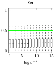
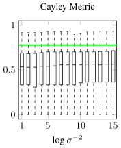
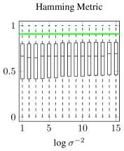
Figure 4: Distances between the optimal sentences with respect to the model and the correct sentences.

Finally, we consider the problem of estimating the linear order of words in sentences. Training data is provided by every well-formed sentence and is therefore abundant. We estimate, for every pair $jj^{\prime}$ of words $j$ and $j^{\prime}$ in a dictionary, the probability of the word $j$ to occur before the word $j^{\prime}$ in a sentence. Our dictionary consists of the 1,000 words most often used in the English Wikipedia. Our training (test) data consists of 129,389 (10,000) sentences, drawn randomly and without replacement from those sentences in the English Wikipedia that contain only words from the dictionary. We define $A$ to be the set of all occurrences of words in a sentence, as the same word can occur multiple times. For every pair $aa^{\prime}$ of occurrences of words, the feature vector $x_{aa^{\prime}}\in\{0,1\}^{J}$ is indexed by $J$, the set of all pairs of words in the dictionary. We define $(x_{aa^{\prime}})_{jj^{\prime}}=1$ iff $a$ is an occurrence of the word $j$ and $a^{\prime}$ is an occurrence of the word $j^{\prime}$. With respect to the Bernoulli model, optimal parameters $\hat{\theta}$ are learned by evaluating the closed form (13), which takes less than 10 seconds for the entire training set. Every sentence of the test set is taken to be an unordered set of words and is permuted randomly for this experiment. An optimal linear order of words is estimated by solving the Linear Ordering Problem, that is, (14), with the feasible set $z$ defined as the set of those $y\in\{0,1\}^{A\times B}$ that satisfy (5.2), (5.2), (5.3) and (5.3). For all instances, we use the branch-and-cut loop of Cplex, separating the inequalities (5.2), (5.2), (5.3) and (5.3) and otherwise resorting to the general classes of cuts implemented in Cplex.

Metric distances between the optimal sentences with respect to the model and the correct sentences are reported for three different metrics [22] in Fig. 4. For the summary statistics in this figure, the metrics have been normalized appropriately to account for the different lengths of sentences. Horizontal lines indicate the value the normalized metric would assume for randomly ordered sentences. It can be seen from this figure that the model is effective in estimating the order of words in sentences and is not sensitive to the regularization parameter $\sigma$ for the dictionary and training data we used.

7 Conclusion

We have defined a family of probability measures on the set of all relations between two finite, non-empty sets which offers a joint abstraction of multi-label classification, correlation clustering and ranking by linear ordering. The problem of estimating (learning) a maximally probable measure, given (a training set of) related and unrelated pairs, is a convex optimization problem. The problem of estimating (inferring) a maximally probable relation, given a measure, is a $01$-linear program which specializes to the NP-hard Set Partition Problem for equivalence relations and to the NP-hard Linear Ordering Problem for linear orders. Experiments with real data have shown that maximum probability learning and maximum probability inference are practical for some instances.

In the experiments we conduct, the distinction between learning and inference is motivated by the distinction between training data and test data. It is well-known, however, that a distinction between learning and inference is inappropriate if there is just one data set and partial evidence about a to-be-estimated relation. With respect to this setting which falls into the broader research area of semi-supervised learning, we have stated the problem of estimating $\theta$ and $x$ jointly as the mixed-integer nonlinear programs (5)–(7) and (10)–(12). Toward a solution of these problems, we understand that a heuristic algorithm that alternates between the optimization of $\theta$ and $x$, aside form solving, in each iteration, a problem that is NP-hard for equivalence relations and linear orders, can have sub-optimal fixed-points. We also understand that the continuous relaxations of the problems are not necessarily (and not typically) convex. We have stated these problems as mixed-integer nonlinear programs in order to foster the exchange of ideas between the machine learning community and the optimization communities.

Appendix A Proofs

A.1 Proof of Lemma 1

From (1) follows

$$\underset{\theta\in\mathbb{R}^{K},y\in\{0,1\}^{A\times B}}{\mathrm{argmax}} \ p_{Y,\Theta|X,Z}(y,\theta,x,z)$$

$$=\underset{\theta\in\mathbb{R}^{K},y\in z}{\mathrm{argmax}}\hskip 12.91663pt \ \prod_{ab\in A\times B}\underbrace{p_{Y_{ab}|X_{ab},\Theta}}_{=:p}(y_{ab},\theta,x_{ab})\cdot\prod_{k\in K}\underbrace{p_{\Theta_{k}}}_{=:q}(\theta_{k})$$

$$=\underset{\theta\in\mathbb{R}^{K},y\in z}{\mathrm{argmax}}\hskip 12.91663pt \ \sum_{ab\in A\times B}\log_{2}p(y_{ab},\theta,x_{ab})+\sum_{k\in K}\log_{2}q(\theta_{k})$$

$$=\underset{\theta\in\mathbb{R}^{K},y\in z}{\mathrm{argmin}}\hskip 12.91663pt \ -\sum_{ab\in A\times B}\Big{(}y_{ab}\log_{2}p(1,\theta,x_{ab})+(1-y_{ab})\log_{2}p(0,\theta,x_{ab})\Big{)}-\sum_{k\in K}\log_{2}q(\theta_{k})$$

$$=\underset{\theta\in\mathbb{R}^{K},y\in z}{\mathrm{argmin}}\hskip 12.91663pt \ -\sum_{ab\in A\times B}\left(y_{ab}\log_{2}\frac{p(1,\theta,x_{ab})}{p(0,\theta,x_{ab})}+\log_{2}p(0,\theta,x_{ab})\right)-\sum_{k\in K}\log_{2}q(\theta_{k})$$

$$=\underset{\theta\in\mathbb{R}^{K},y\in z}{\mathrm{argmin}}\hskip 12.91663pt \ \sum_{ab\in A\times B}\left(y_{ab}\log_{2}\frac{p(0,\theta,x_{ab})}{p(1,\theta,x_{ab})}-\log_{2}p(0,\theta,x_{ab})\right)-\sum_{k\in K}\log_{2}q(\theta_{k})\enspace.$$ (22)

From (22) and (3) follows

$$\underset{\theta\in\mathbb{R}^{K},y\in\{0,1\}^{A\times B}}{\mathrm{argmax}} \ p_{Y,\Theta|X,Z}(y,\theta,x,z)$$

$$=\underset{\theta\in\mathbb{R}^{K},y\in z}{\mathrm{argmin}}\hskip 12.91663pt \quad\sum_{ab\in A\times B}\left(-y_{ab}\langle\theta,x_{ab}\rangle+\log_{2}\left(1+2^{\langle\theta,x_{ab}\rangle}\right)\right)+|K|\log_{2}(\sigma\sqrt{2\pi})+\frac{\log_{2}e}{2\sigma^{2}}\|\theta\|_{2}^{2}$$

$$=\underset{\theta\in\mathbb{R}^{K},y\in z}{\mathrm{argmin}}\hskip 12.91663pt \quad\sum_{ab\in A\times B}\left(-y_{ab}\langle\theta,x_{ab}\rangle+\log_{2}\left(1+2^{\langle\theta,x_{ab}\rangle}\right)\right)+\frac{\log_{2}e}{2\sigma^{2}}\|\theta\|_{2}^{2}\enspace.$$ (23)

Partial derivatives of the function $D_{x}$ defined in (6) with respect to $\theta\in\mathbb{R}^{K}$ and $y\in(0,1)^{A\times B}$ are

$$(\partial_{\theta_{j}}D_{x})(\theta,y) =\sum_{ab\in A\times B}(x_{ab})_{j}\left(-y_{ab}+\frac{1}{1+2^{-\langle\theta,x_{ab}\rangle}}\right)$$ (24)

$$(\partial_{y_{ab}}D_{x})(\theta,y) =-\langle\theta,x_{ab}\rangle$$ (25)

$$(\partial_{\theta_{j},\theta_{k}}D_{x})(\theta,y) =\sum_{ab\in A\times B}(x_{ab})_{j}(x_{ab})_{k}\underbrace{\frac{2^{\langle\theta,x_{ab}\rangle}\log_{e}2}{\left(1+2^{\langle\theta,x_{ab}\rangle}\right)^{2}}}_{=:\xi_{ab}^{2}}$$ (26)

$$(\partial_{\theta_{j},y_{ab}}D_{x})(\theta,y)=(\partial_{y_{ab},\theta_{j}}D_{x})(\theta,y) =-(x_{ab})_{j}$$ (27)

$$(\partial_{y_{ab},y_{a^{\prime}b^{\prime}}}D_{x})(\theta,y) =0\enspace.$$ (28)

Thus, the Hessian of $D_{x}$ is of the special form

$$H=\left[\begin{array}[]{cc}H_{\theta\theta}&H_{\theta y}\\ H_{\theta y}^{T}&0\end{array}\right]\qquad\textnormal{with}\qquad H_{\theta\theta}=\sum\limits_{ab\in A\times B}(\xi_{ab}x_{ab})(\xi_{ab}x_{ab})^{T}\enspace.$$ (31)

It defines the quadratic form

$$\left[\theta^{T}\ y^{T}\right]H\left[\begin{array}[]{c}\theta\\ y\end{array}\right]=\log_{e}(2)\sum_{ab\in A\times B}\frac{2^{\langle\theta,x_{ab}\rangle}}{\left(1+2^{\langle\theta,x_{ab}\rangle}\right)^{2}}\langle\theta,x_{ab}\rangle^{2}-2\sum_{ab\in A\times B}y_{ab}\langle\theta,x_{ab}\rangle\enspace.$$ (34)

This quadratic form need not be positive semi-definite. Thus, $D_{x}$ need not be a convex function. However, the Hessian $H_{\theta\theta}$ of the function $D_{x}(\cdot,\hat{y})$ is positive semi-definite for any fixed $\hat{y}\in[0,1]^{A\times B}$. Thus, the function $D_{x}(\cdot,\hat{y})$ is convex.

A.2 Proof of Lemma 3

From (22) and (3) follows

$$\underset{\theta\in\mathbb{R}^{K},y\in\{0,1\}^{A\times B}}{\mathrm{argmax}} \ p_{Y,\Theta|X,Z}(y,\theta,x,z)$$

$$=\underset{\theta\in\mathbb{R}^{K},y\in z}{\mathrm{argmin}}\hskip 12.91663pt \ \sum_{ab\in A\times B}\left(y_{ab}\log_{2}\frac{\prod_{j\in J}(1-\theta_{j})^{{(x_{ab})}_{j}}}{\prod_{j\in J}\theta_{j}^{{(x_{ab})}_{j}}}-\log_{2}\prod_{j\in J}(1-\theta_{j})^{{(x_{ab})}_{j}}\right)$$

$$\ -\sum_{j\in J}\log_{2}\frac{\Gamma(2\sigma)}{\Gamma^{2}(\sigma)}\theta_{j}^{\sigma-1}(1-\theta_{j})^{\sigma-1}$$

$$=\underset{\theta\in\mathbb{R}^{K},y\in z}{\mathrm{argmin}}\hskip 12.91663pt \ \sum_{ab\in A\times B}\left(y_{ab}\log_{2}\prod_{j\in J}\left(\frac{1-\theta_{j}}{\theta_{j}}\right)^{{(x_{ab})}_{j}}-\sum_{j\in J}{(x_{ab})}_{j}\log_{2}(1-\theta_{j})\right)$$

$$\ -|J|\log_{2}\frac{\Gamma(2\sigma)}{\Gamma^{2}(\sigma)}-(\sigma-1)\sum_{j\in J}\log_{2}\theta_{j}(1-\theta_{j})$$

$$=\underset{\theta\in\mathbb{R}^{K},y\in z}{\mathrm{argmin}}\hskip 12.91663pt \ \sum_{ab\in A\times B}\left(\left(\sum_{j\in J}{(x_{ab})}_{j}\log_{2}\frac{1-\theta_{j}}{\theta_{j}}\right)y_{ab}-\sum_{j\in J}{(x_{ab})}_{j}\log_{2}(1-\theta_{j})\right)$$

$$\ +(1-\sigma)\sum_{j\in J}\log_{2}\theta_{j}(1-\theta_{j})\enspace.$$ (35)

The form $D_{x}(\theta,y)$ defined in (11) is equivalent to the form below.

$$D_{x}(\theta,y) =-\sum_{j\in J}\left(\log(1-\theta_{j})\sum_{ab\in A\times B}(x_{ab})_{j}(1-y_{ab})+\log(\theta_{j})\sum_{ab\in A\times B}(x_{ab})_{j}y_{ab}\right)$$ (36)

$$=-\sum_{j\in J}\left(m_{j}^{-}\log(1-\theta_{j})+m_{j}^{+}\log\theta_{j}\right)\enspace.$$ (37)

Partial derivarives of $D_{x}$ with respect to $\theta\in(0,1)^{K}$ and $y\in(0,1)^{A\times B}$ are

$$(\partial_{\theta_{j}}D_{x})(\theta,y) =\frac{1}{\log_{e}2}\left(\frac{m_{j}^{-}}{1-\theta_{j}}-\frac{m_{j}^{+}}{\theta_{j}}\right)$$ (38)

$$(\partial_{y_{ab}}D_{x})(\theta,y) =\sum_{j\in J}(x_{ab})_{j}\log_{2}\frac{1-\theta_{j}}{\theta_{j}}$$ (39)

$$(\partial_{\theta_{j},\theta_{k}}D_{x})(\theta,y) =\frac{\delta_{jk}}{\log_{e}2}\left(\frac{m_{j}^{-}}{(1-\theta_{j})^{2}}+\frac{m_{j}^{+}}{\theta_{j}^{2}}\right)$$ (40)

$$(\partial_{\theta_{j},y_{ab}}D_{x})(\theta,y)=(\partial_{y_{ab},\theta_{j}}D_{x})(\theta,y) =\frac{-1}{\log_{e}2}\frac{(x_{ab})_{j}}{(1-\theta_{j})\theta_{j}}$$ (41)

$$(\partial_{y_{ab},y_{a^{\prime}b^{\prime}}}D_{x})(\theta,y) =0$$ (42)

Thus, the Hessian of $D_{x}$ is of the special form

$$H=\left[\begin{array}[]{cc}H_{\theta\theta}&H_{\theta y}\\ H_{\theta y}^{T}&0\end{array}\right]\qquad\textnormal{with}\qquad(H_{\theta\theta})_{jk}=\frac{\delta_{jk}}{\log_{e}2}\left(\frac{m_{j}^{-}}{(1-\theta_{j})^{2}}+\frac{m_{j}^{+}}{\theta_{j}^{2}}\right)\enspace.$$ (45)

It defines the quadratic form

$$\left[\theta^{T}\ y^{T}\right]H\left[\begin{array}[]{c}\theta\\ y\end{array}\right]=\frac{1}{\log_{e}2}\sum_{j\in J}\left(\frac{\theta_{j}^{2}}{(1-\theta_{j})^{2}}m_{j}^{-}-\frac{1+\theta_{j}}{1-\theta_{j}}m_{j}^{+}\right)\enspace.$$ (48)

This quadratic form need not be positive semi-definite. Thus, $D_{x}$ need not be a convex function. However, the Hessian $H_{\theta\theta}$ of the function $D_{x}(\cdot,\hat{y})$ is positive semi-definite for any fixed $\hat{y}\in[0,1]^{A\times B}$. Thus, the function $D_{x}(\cdot,\hat{y})$ is convex.

A.3 Proof of Lemma 2

Proof.

Let $ab\in A\times B$ arbitrary and fixed. If $\hat{y}_{ab}=0$,

$$0\ =\ \log_{2}1\ <\ \log_{2}\left(1+2^{\langle\hat{\theta},x_{ab}\rangle}\right)\ =\ \hat{y}_{ab}\langle\hat{\theta},x_{ab}\rangle+\log_{2}\left(1+2^{\langle\hat{\theta},x_{ab}\rangle}\right)\enspace.$$

If $\hat{y}_{ab}=1$,

$$0=-\langle x_{ab},\theta\rangle+\langle x_{ab},\theta\rangle=-\hat{y}_{ab}\langle x_{ab},\theta\rangle+\log_{2}2^{\langle x_{ab},\theta\rangle}<-\hat{y}_{ab}\langle x_{ab},\theta\rangle+\log_{2}\left(1+2^{\langle x_{ab},\theta\rangle}\right)\enspace.$$

That is, every summand in the form (6) of $D_{x}$ is bounded from below by 0. Therefore, $0<D_{x}$ and thus, the infimum exists. Moreover, for any $y\in\{0,1\}^{A\times B}$, $\inf_{\theta,\hat{y}}D_{x}(\theta,\hat{y})\leq D(0,y)=|A||B|$, which establishes the upper bound.

Appendix B Multilinear Polynomial Lifting

B.1 Exact

Definition 1.

For any finite index set $J$, the multilinear polynomial lifting of $\{0,1\}^{J}$ is the map $l:\{0,1\}^{J}\to\{0,1\}^{2^{J}}$ such that $\forall v\in\{0,1\}^{J}\ \forall J^{\prime}\subseteq J$:

$$l(v)_{J^{\prime}}=\prod_{j\in J^{\prime}}v_{j}\enspace.$$ (49)

For example, consider $J=\{1,2\}$ and $l:(v_{1},v_{2})\mapsto(1,v_{1},v_{2},v_{1}v_{2})$.

Lemma 4.

A one-to-one correspondence between functions $f:\{0,1\}^{J}\to\mathbb{R}$ and vectors $\theta\in\mathbb{R}^{2^{J}}$ is established by defining $\forall v\in\{0,1\}^{J}$:

$$f(v)=\langle\theta,l(v)\rangle\enspace.$$ (50)

Proof.

By Proposition 2 in [15].

For example, consider $J=\{1,2\}$ and $f(v)=\theta_{0}+\theta_{1}v_{1}+\theta_{2}v_{2}+\theta_{12}v_{1}v_{2}$.

Lemma 5.

A one-to-one correspondence between functions $p:\{0,1\}^{J}\to(0,1)$ and functions $f:\{0,1\}^{J}\to\mathbb{R}$ is established by defining $\forall v\in\{0,1\}^{J}$:

$$p(v)=\left(1+2^{-f(v)}\right)^{-1}\enspace.$$ (51)

Proof.

Trivial.

With respect to (50) and (51) and the prior in (3), the problem (22) of estimating a $p_{Y_{ab}|X_{ab},\Theta}:\{0,1\}^{J}\to(0,1)$ and a $y\in\{0,1\}^{A\times B}$ so as to maximize (1) can be written in the functional form below and, thus, in the parametric form (5)–(7).

$$\min_{f:\{0,1\}^{J}\to\mathbb{R}}\mathcal{D}(f)+\mathcal{R}_{\sigma}(f)$$ (52)

$$\mathcal{D}(f) :=\sum_{ab\in A\times B}\left(-\langle\theta(f),l(x_{ab})\rangle y_{ab}+\log_{2}\left(1+2^{\langle\theta(f),l(x_{ab})\rangle}\right)\right)$$ (53)

$$\mathcal{R}_{\sigma}(f) :=R_{\sigma}(\theta(f))$$ (54)

B.2 Approximate

Solving for the $2^{|J|}$ parameters $\theta$ in (52)–(54) is impractical for sufficiently large $|J|$. To address this problem, we approximate the multi-linear polynomial form (50) for fixed $d,m\in\mathbb{N}$, by a linear form $\langle\theta^{\prime},l^{\prime}(x)\rangle$ where $l^{\prime}:\{0,1\}^{J}\to\mathbb{Z}^{m}$ is drawn randomly from the distribution defined in [16], such that the inner product $\langle l^{\prime}(x),l^{\prime}(x^{\prime})\rangle$ approximates the polynomial kernel $k(x,x^{\prime})=(1+\langle x,x^{\prime}\rangle)^{d}$.

This approximation of the multi-variate polynomial lifting approximates the multi-linear polynomial lifting (49) and thus, the multi-linear polynomial form (50), because every multi-linear polynomial form is a multi-variate polynomial form, and every multi-variate polynomial form in $\{0,1\}^{J}$ is equivalent to a multi-linear polynomial form in $\{0,1\}^{J}$ (because exponents are irrelevant).

Appendix C One-Versus-Rest Classification

Lemma 6.

Let $v:A\to\{0,1\}^{J}$ arbitrary and fixed. Let $x:A\times B\to\{0,1\}^{J\cup B}$ such that, for any $ab\in A\times B$, firstly, $(x_{ab})_{J}=v_{J}$ and, secondly, for all $b^{\prime}\in B$, $(x_{ab})_{b^{\prime}}=1$ iff $b^{\prime}=b$. Let

$$\mathcal{F} =\left\{f:\{0,1\}^{J\cup B}\to\mathbb{R}\ \middle|\ \exists g:B\to\mathbb{R}^{\{0,1\}^{J}}\forall w\in\{0,1\}^{J\cup B}:f(w)=\sum_{b\in B}w_{b}g_{b}(w_{J})\right\}\ .$$ (55)

Then, $\hat{f}\in\underset{f\in\mathcal{F}}{\mathrm{argmin}}\ \mathcal{D}_{x}(f)+\mathcal{R}_{\sigma}(f)$ iff, for every $b\in B$,

$$\hat{g}_{b}\in\underset{g_{b}:\{0,1\}^{J}\to\mathbb{R}}{\mathrm{argmin}}\ \sum_{a\in A}\left(-g_{b}(v_{a})y_{ab}+\log_{2}\left(1+2^{g_{b}(v_{a})}\right)\right)+\mathcal{R}_{\sigma}(g_{b})\enspace.$$ (56)

Proof.

Let $J^{\prime}\subseteq J\cup B$. If $|J^{\prime}\cap B|\not=1$ then $\theta(f)_{J^{\prime}}=0$ by (55). Otherwise, there exists a unique $b\in J^{\prime}\cap B$ and $\theta(f)_{J^{\prime}}=\theta(g_{b})_{J^{\prime}}$ by (55). Thus, $\mathcal{R}_{\sigma}(f)=\sum_{b\in B}\mathcal{R}_{\sigma}(g_{b})$. Moreover,

$$\mathcal{D}_{x}(f) =\sum_{ab\in A\times B}\left(-f(x_{ab})y_{ab}+\log_{2}\left(1+2^{f(x_{ab})}\right)\right)$$

$$=\sum_{ab\in A\times B}\left(-\left(\sum_{b^{\prime}\in B}(x_{ab})_{b^{\prime}}g_{b}((x_{ab})_{J})\right)y_{ab}+\log_{2}\left(1+2^{\left(\sum_{b^{\prime}\in B}(x_{ab})_{b^{\prime}}g_{b}((x_{ab})_{J})\right)}\right)\right)$$

$$=\sum_{b\in B}\left(\sum_{a\in A}\left(-g_{b}(v_{a})y_{ab}+\log_{2}\left(1+2^{g_{b}(v_{a})}\right)\right)\right)\enspace.$$

Lemma 7.

Let $\hat{\theta}\in\mathbb{R}^{A\times B}$ arbitrary and fixed. Call $y\in\{0,1\}^{A\times B}$ a local solution iff, for all $a\in A$, there exists a $b_{a}\in B$ such that, firstly, $b_{a}\in\mathrm{argmin}_{b^{\prime}\in B}-\langle\hat{\theta},x_{ab^{\prime}}\rangle$ and, secondly, $\forall b\in B:y_{ab}=1\Leftrightarrow b=b_{a}$. Then, $y$ is a solution iff it is a local solution.

Proof.

Any local solution is obviously feasible. Any local solution is optimal because

$$\quad\min_{\{y\in\{0,1\}^{A\times B}|y\in z\}}-\sum_{ab\in A\times B}\langle\hat{\theta},x_{ab}\rangle y_{ab}$$

$$= \quad\sum_{a\in A}\min_{\{y_{a\cdot}\in\{0,1\}^{B}|y\in z\}}-\langle\hat{\theta},x_{ab}\rangle y_{ab}$$

$$= \quad\sum_{a\in A}\min_{b\in B}-\langle\hat{\theta},x_{ab}\rangle y_{ab}\enspace.$$

Appendix D Features of Pairs

Consider the problem of estimating a relation on a set $A$, say, an equivalence relation or a linear order. Instead of a feature vector for every pair $aa^{\prime}\in A\times A$, that is, instead of $x:A\times A\to\{0,1\}^{J}$, we may be given a feature vector for every element $a\in A$, that is, $w:A\to\{0,1\}^{L}$.

Now, we need to define, for each pair $aa^{\prime}$, a feature vector $x_{aa^{\prime}}\in\{0,1\}^{J}$ with respect to $w_{a}$ and $w_{a^{\prime}}$. Ideally, $x_{aa^{\prime}}$ should be invariant under transposition of $w_{a}$ and $w_{a^{\prime}}$ and otherwise general. Our restriction to $01$-features affords a simple definition which has this property. For every $01$-feature of elements, indexed by $l\in L$, two $01$-features of pairs, indexed by $j_{l1},j_{l2}\in J$, are defined as

$$(x_{aa^{\prime}})_{j_{l1}} :=(v_{a})_{l}(v_{a^{\prime}})_{l}$$ (57)

$$(x_{aa^{\prime}})_{j_{l2}} :=(v_{a})_{l}+(v_{a^{\prime}})_{l}-2(v_{a})_{l}(v_{a^{\prime}})_{l}$$ (58)

These $01$-features are invariant under transposition of $v_{a}$ and $v_{a^{\prime}}$. Moreover, the multilinear polynomial forms in $x_{aa^{\prime}}$ comprise the basic transposition invariant multilinear polynomial forms

$$(v_{a})_{l}(v_{a^{\prime}})_{l} =(x_{aa^{\prime}})_{j_{l1}}$$ (59)

$$(v_{a})_{l}+(v_{a^{\prime}})_{l} =(x_{aa^{\prime}})_{j_{l2}}+2(x_{aa^{\prime}})_{j_{l1}}\enspace.$$ (60)

Appendix E Complementary Experiments

E.1 Maps (Classification)

Figure 5: Absolute computation times for the classification of images of handwritten digits (MNIST). Colors have the same meaning as in Fig. 2. Symbols indicate 8192 (${\color[rgb]{0,0,1}+},{\color[rgb]{0,1,0}+}$) and 16384 (${\color[rgb]{0,0,1}\bullet},{\color[rgb]{0,1,0}\bullet}$) random features, respectively.

For the classification of images of handwritten digits, absolute computation times are depicted in Fig. 5. It can be seen from this figure that it takes less than $10^{4}$ seconds to estimate (learn) all parameters of the probability measure from the entire MNIST training set, using the open-source software [17] to solve the convex learning problem. It can also be seen from this figure that it takes less than $10^{3}$ seconds to estimate (infer) the labels of all images of the MNIST test set, using our (trivial) C++ code to solve the (trivial) inference problem.

E.2 Equivalence Relations (Clustering)

Toward the clustering of sets of images of handwritten digits, we reconsider the problem of classifying pairs of images as either showing or not showing the same digit. A pair $aa^{\prime}$ of images $a$ and $a^{\prime}$ is labeled with $y_{aa^{\prime}}=1$ if the images show (are labeled with) the same digit. It is labeled with $y_{aa^{\prime}}=0$, otherwise. Analogous to the experiment described in Section 6.2, we now collect an unstratified training set $\{(x_{aa^{\prime}},y_{aa^{\prime}})\}_{aa^{\prime}\in T}$ by drawing $|T|=5\cdot 10^{5}$ pairs of images randomly, without replacement, from the MNIST training set. As the MNIST training set contains (about) equally many images for each of 10 digits, the label $y_{aa^{\prime}}=0$ is (about) 9 times as abundant in $T$ as the label $y_{aa^{\prime}}=1$. A test set of the same cardinality is drawn analogously from the MNIST test set. Results for the independent classification of pairs (not a solution of the Set Partition Problem) are shown in Fig. 6. It can be seen from this figure that the fraction of misclassified pairs is 7.45% for the unstratified test data, at $\sigma^{-2}=2^{21}$ and for an approximation of a multilinear polynomial form of degree $d=2$ by 16384 random features.

For $\hat{\theta}$ learned with these parameters, we infer equivalence relations on random subsets $A$ of the MNIST test set by solving the Set Partition Problem as described in Section 6.2. An evaluation analogous to Section 6.2 is shown in Tab. 2. In comparison with Tab. 1, it can be seen that the inferred equivalence relations on previously unseen test sets have a smaller fraction $e_{\mathrm{RI}}$ of misclassified pairs when learning from unstratified (biased) training data. However, they are worse in terms of the Variation of Information, number of sets and objective value. This shows empirically that training data in this setting should be stratified.

Figure 6: Classification of pairs of images of handwritten digits (MNIST). Colors and line styles have the same meaning as in Fig. 2.

Figure 7: Absolute computation times for the classification of pairs of handwritten digits (learning and inference).

Table 2: Comparison of equivalence relations on unstratified random subsets $A$ of the MNIST test set

		$|A|$	${|A|\choose 2}$	$e_{\mathrm{RI}}\ [\%]$	$\mathrm{VI}$ [21]	Sets	Obj./${|A|\choose 2}\cdot 10^{2}$	$t\ [s]$
$\hat{\theta}$	$\hat{y}$	100	4950	$6.36$ $\pm$ $0.74$	$\bf 1.35$ $\pm$ $0.19$	$43.0$ $\pm$ $5.8$	$-3.84$ $\pm$ $1.17$	$\bf 3.23$	$\pm$	$2.29$
		170	14365	$6.48$ $\pm$ $0.38$	$\bf 1.56$ $\pm$ $0.10$	$64.1$ $\pm$ $5.7$	$-3.76$ $\pm$ $0.66$	$\bf 5.75$	$\pm$	$4.21$
		220	24090	$6.81$ $\pm$ $0.41$	$\bf 1.75$ $\pm$ $0.12$	$77.8$ $\pm$ $3.5$	$-3.51$ $\pm$ $0.55$	$\bf 12.05$	$\pm$	$9.25$
		260	33670	$6.85$ $\pm$ $0.35$	$\bf 1.82$ $\pm$ $0.12$	$89.4$ $\pm$ $5.9$	$-3.46$ $\pm$ $0.53$	$\bf 26.97$	$\pm$	$26.25$
		300	44850	$6.57$ $\pm$ $0.22$	$\bf 1.79$ $\pm$ $0.09$	$94.8$ $\pm$ $7.2$	$-3.68$ $\pm$ $0.30$	$\bf 107.71$	$\pm$	$129.69$
	$\hat{y}^{\mathrm{KL}}$	100	4950	$6.40$ $\pm$ $0.76$	$\bf 1.36$ $\pm$ $0.19$	$43.0$ $\pm$ $5.9$	$-3.84$ $\pm$ $1.17$	$\bf 0.01$	$\pm$	$0.00$
		170	14365	$6.46$ $\pm$ $0.42$	$\bf 1.56$ $\pm$ $0.12$	$63.8$ $\pm$ $5.9$	$-3.75$ $\pm$ $0.67$	$\bf 0.03$	$\pm$	$0.01$
		220	24090	$6.80$ $\pm$ $0.44$	$\bf 1.75$ $\pm$ $0.13$	$77.3$ $\pm$ $4.1$	$-3.50$ $\pm$ $0.56$	$\bf 0.06$	$\pm$	$0.02$
		260	33670	$6.85$ $\pm$ $0.37$	$\bf 1.83$ $\pm$ $0.14$	$89.4$ $\pm$ $6.2$	$-3.46$ $\pm$ $0.53$	$\bf 0.09$	$\pm$	$0.03$
		300	44850	$6.55$ $\pm$ $0.22$	$\bf 1.78$ $\pm$ $0.09$	$94.5$ $\pm$ $7.0$	$-3.68$ $\pm$ $0.30$	$\bf 0.15$	$\pm$	$0.04$
		$\bf 10^{4}$	$\bf 5\cdot 10^{9}$	$\bf 6.69$	$\bf 2.88$	$\bf 1168$	$\bf-3.74$	$\bf 1340.70$

E.3 Orders (Ranking)

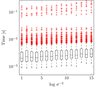
Figure 8: Absolute computation time for linear ordering of words in sentences (inference).

For the linear ordering of words in sentences, absolute computation times are summarized in Fig. 8.

References

- [1] Gükhan H. Bakır, Thomas Hofmann, Bernhard Schölkopf, Alexander J. Smola, Ben Taskar, and S. V. N. Vishwanathan. Predicting Structured Data. MIT Press, 2007.
- [2] Ioannis Tsochantaridis, Thorsten Joachims, Thomas Hofmann, Yasemin Altun, and Yoram Singer. Large margin methods for structured and interdependent output variables. JMLR, 6(9), 2005.
- [3] Tilman Lange, Martin H. C, Law Anil, K. Jain, and Joachim M. Buhmann. Learning with constrained and unlabeled data. In CVPR, pages 731–738, 2005.
- [4] Sunil Chopra and M. R. Rao. The partition problem. Mathematical Programming, 59(1–3):87–115, 1993.
- [5] Nikhil Bansal, Avrim Blum, and Shuchi Chawla. Correlation clustering. Machine Learning, 56(1–3):89–113, 2004.
- [6] Erik D. Demaine, Dotan Emanuel, Amos Fiat, and Nicole Immorlica. Correlation clustering in general weighted graphs. Theoretical Computer Science, 361(2):172–187, 2006.
- [7] Michel M. Deza and Monique Laurent. Geometry of Cuts and Metrics. Springer, 1997.
- [8] Eric P. Xing, Andrew Y. Ng, Michael I. Jordan, and Stuart Russell. Distance metric learning with application to clustering with side-information. NIPS, pages 521–528, 2003.
- [9] Bjoern Andres, Jörg H. Kappes, Thorsten Beier, Ullrich Köthe, and Fred A. Hamprecht. Probabilistic image segmentation with closedness constraints. In ICCV, 2011.
- [10] Bjoern Andres, Thorben Kroeger, Kevin L. Briggman, Winfried Denk, Natalya Korogod, Graham Knott, Ullrich Koethe, and Fred A Hamprecht. Globally optimal closed-surface segmentation for connectomics. In ECCV, 2012.
- [11] Jörg H. Kappes, Markus Speth, Gerhard Reinelt, and Christoph Schnörr. Higher-order segmentation via multicuts. ArXiv e-prints, 2013.
- [12] Sungwoong Kim, Chang D. Yoo, Sebastian Nowozin, and Pushmeet Kohli. Image segmentation using higher-order correlation clustering. PAMI, PP(99), 2014.
- [13] Rafael Martí and Gerhard Reinelt. The Linear Ordering Problem. Springer, 2011.
- [14] Roy Tromble and Jason Eisner. Learning linear ordering problems for better translation. In Proceedings of the 2009 Conference on Empirical Methods in Natural Language Processing, pages 1007–1016, Stroudsburg, PA, USA, 2009. Association for Computational Linguistics.
- [15] Endre Boros and Peter L. Hammer. Pseudo-boolean optimization. Discrete Applied Mathematics, 123(1–3):155–225, 2002.
- [16] Ninh Pham and Rasmus Pagh. Fast and scalable polynomial kernels via explicit feature maps. In KDD, pages 239–247, 2013.
- [17] Rong-En Fan, Kai-Wei Chang, Cho-Jui Hsieh, Xiang-Rui Wang, and Chih-Jen Lin. LIBLINEAR: A library for large linear classification. JMLR, 9:1871–1874, 2008.
- [18] Brian W. Kernighan and Shen Lin. An efficient heuristic procedure for partitioning graphs. Bell system technical journal, 49(2):291–307, 1970.
- [19] Yann LeCun and Corinna Cortes. The mnist database of handwritten digits, 1998.
- [20] Li Wan, Matthew Zeiler, Sixin Zhang, Yann LeCun, and Rob Fergus. Regularization of neural networks using dropconnect. In ICML, 2013.
- [21] Marina Meilă. Comparing clusterings by the variation of information. In Learning theory and kernel machines, pages 173–187. 2003.
- [22] Michael Deza and Tayuan Huang. Metrics on permutations, a survey. In Journal of Combinatorics, Information and System Sciences, 1998.