Target Detection Performance of Spectrum Sharing MIMO Radars
Abstract
Future wireless communication systems are envisioned to share radio frequency (RF) spectrum, with other services such as radars, in order to meet the growing spectrum demands. In this paper, we consider co-channel spectrum sharing between cellular systems and radars. We address the problem of target detection by radars that are subject to shape its waveform in a way that it doesn’t cause interference to cellular systems. We consider a multiple-input multiple-output (MIMO) radar and a MIMO cellular communication system with base stations (BS). We propose a spectrum sharing algorithm which steers radar nulls, by projecting radar waveform onto the null space of interference channel, towards a ‘selected’ BS, thus, protecting it from radar interference. This BS is selected, among BSs, on the basis of guaranteeing minimum waveform degradation. We study target detection capabilities of this null-space projected (NSP) waveform and compare it with the orthogonal waveform. We derive the generalized likelihood ratio test (GLRT) for target detection and derive detector statistic for NSP and orthogonal waveform. The target detection performance for NSP and orthogonal waveform is studied theoretically and via Monte Carlo simulations.
Index Terms:
MIMO Radar, Null Space Projection, Cellular System Coexistence, Target Detection, GLRT, ML Estimation.I Introduction
Spectrum sharing between wireless communication systems and radars is an emerging area of research. In the past, spectrum has been shared primarily between wireless communication systems using opportunistic approaches by users equipped with cognitive radios [1]. This type of spectrum sharing has been made possible with the use of spectrum sensing [2], or geolocation databases [3], or a combination of both in the form of radio environment maps (REM) [4]. Some recent efforts have explored co-channel sharing approaches among secondary network entities, please see [5] and reference therein. However, in contrast, co-channel spectrum sharing between wireless systems and radars has received little attention thus far because of regulatory concerns.
Spectrum policy regulators, in the past, have not allowed commercial wireless services in the radar bands, except in few cases, due to the fear of harmful interference from these services to radar systems. Recently, in the United States (U.S.), the Federal Communications Commission (FCC), has proposed to use the 3550-3650 MHz band for commercial broadband use [6]. The incumbents in this band are radar and satellite systems. The Commission has proposed that incumbents share this band with commercial communication systems. The Commission’s spectrum sharing initiative is motivated by many factors including the President’s National Broadband plan, which called to free up to 500 MHz of federal-held spectrum by 2020 [7]; surge in consumers’ demand for access to mobile broadband, which operators can’t meet with current spectrum allocation; the report on efficient spectrum utilization by President’s Council of Advisers on Science and Technology (PCAST), which emphasized to share 1000 MHz of government-held spectrum [8], and the low utilization of 3550-3650 MHz band by federal incumbents [9].
In the future, when radio frequency (RF) spectrum will be shared among many different systems, e.g., radars and cellular systems, it is important to access the interference scenario. Of course, radars will cause interference to communication systems and vice versa if proper interference mitigation methods and novel sharing algorithms are not employed. In a study conducted by National Telecommunications and Information Administration (NTIA), it was observed that in order to protect commercial cellular communication systems, from high power radar signal, large exclusion zones are required [9]. These exclusion zones cover a large portion of the U.S. where majority of the population lives and, thus, does not make a business case for commercial deployment in radar bands. In order to share radar bands for commercial operation we have to address the interference mitigation techniques at both the systems. In this work, we focus on interference caused by radar systems to communication system and propose methods to mitigate this interference.
The federal-commercial spectrum sharing is not a new practice. In fact, in the past, commercial wireless systems have shared government bands on a low transmit power basis, in order to protect incumbents from interference. An example of such a scenario is wireless local area network (WLAN) in the 5250-5350 MHz and 5470-5725 MHz radar bands [10]. So the Commission’s latest initiative to share 3.5 GHz radar band with small cells, i.e. wireless base stations operating on a low power, is in harmony with previous practices [6].
I-A Related Work
On going research efforts have shown that there are numerous ways to share spectrum between radars and communication systems. Cooperative sensing based spectrum sharing approaches can be utilized where a radar’s allocated bandwidth is shared with communication systems [11, 12, 13]. A joint communication-radar platform can be envisioned in which a spectrally-agile radar performs an additional task of spectrum sensing and upon finding of unused frequencies it can change its operating frequency. In addition of spectrum sharing such a setting can enable co-located radar and communication system platforms for integrated communications and radar applications [14, 15, 16, 17]. Radar waveforms can be shaped in a way that they don’t cause interference to communication systems [18, 19, 20, 21, 22, 23]. Moreover, database-aided sensing at communication systems [24] and beamforming approaches at MIMO radars can be realized for spectrum sharing [25].
I-B Our Contributions
The problem of target estimation, detection, and tracking lies at the heart of radar signal processing. This problem becomes critically important when we talk about sharing radar spectrum with other systems, say cellular systems. The regulatory work going on in the 3.5 GHz band to share radar spectrum with commercial systems is the motivation of this work. The focus of this work is to study target detection performance of a radar that is subject to share its spectrum with a cellular system. We consider spectrum sharing between a MIMO radar and a cellular system with many base stations. In our previous work, we have addressed the problem of radar waveform projection onto the null space of interference channel, in order to mitigate radar interference to communication system, and the problem of selection of interference channel for projection when we have a cellular system with base stations [19]. In this work, we consider the same sharing scenario but study the target detection performance of radar for the null-space projected (NSP) waveform and compare it with that of the orthogonal radar waveform. We use the generalized likelihood ratio test (GLRT) for target detection and derive detector statistic for NSP and the orthogonal waveform.
I-C Notations
Matrices are denoted by bold upper case letters, e.g. , and vectors are denoted by bold lower case letters, e.g. . Transpose, conjugate, and Hermitian operators are denoted by and , respectively. Moreover, notations used throughout the paper are provided in Table I along with descriptions for quick reference.
| Notation | Description |
|---|---|
| Transmitted radar (orthogonal) waveform | |
| Steering vector to steer signal to target angle | |
| Received radar waveform | |
| Correlation matrix of orthogonal waveforms | |
| Signal transmitted by the UE in the cell | |
| Total number of user equipments (UEs) in the cell | |
| Total number of BSs | |
| Radar transmit/receive antennas | |
| BS transmit/receive antennas | |
| interference channel | |
| Received signal at the BS | |
| Projection matrix for the channel |
I-D Organization
This paper is organized as follows. Section II discuss MIMO radar, target channel, orthogonal waveforms, interference channel, and our cellular system model. Moreover, it also discusses modeling and statistical assumptions. Section III discusses spectrum sharing between MIMO radar and cellular system and introduces sharing architecture and projection algorithms. Section IV presents the generalized likelihood ratio test (GLRT) for target detection and derives detector statistic for NSP and orthogonal waveform. Section V discusses numerical results and compares performance of NSP and orthogonal waveform. Section VI concludes the paper.
II System Model
In this section, we introduce preliminaries of MIMO radar, point target in far-field, orthogonal waveforms, interference channel, and cellular system model. Moreover, we also discuss modeling and statistical assumptions along with RF environment assumptions used throughout the paper.
II-A Radar Model
The radar we consider in this paper is a colocated MIMO radar with transmit and receive antennas and is mounted on a ship. The colocated MIMO radar has antennas that have spacing on the order of half the wavelength. Another class of MIMO radar is widely-spaced MIMO radar where elements are widely-spaced which results in enhanced spatial diversity [26]. The colocated radar gives better spatial resolution and target parameter identification as compared to the widely-spaced radar [27].
II-B Target Model/Channel
In this paper, we consider a point target model which is defined for targets having a scatterer with infinitesimal spatial extent. This model is a good assumption and is widely used in radar theory for the case when radar elements are colocated and their exists a large distance between the radar array and the target as compared to inter-element distance [28]. The signal reflected from a point target with unit radar cross-section (RCS) is mathematically represented by the Dirac delta function.
II-C Signal Model
Let be the signal transmitted from the -element MIMO radar array, defined as
| (1) |
where is the baseband signal from the transmit element, is the carrier angular frequency, , with being the observation time. We define the transmit steering vector as
| (2) |
Then, the transmit-receive steering matrix can be written as
| (3) |
Since, we are considering transmit and receive elements, we define . The signal received from a single point target, in far-field with constant radial velocity , at an angle can be written as
| (4) |
where , denoting the sum of propagation delays between the target and the transmit element and the receive element, respectively; is the Doppler frequency shift, and represents the complex path loss including the propagation loss and the coefficient of reflection.
II-D Modeling Assumptions
In order to keep the analysis tractable we have made the following assumptions about our signal model:
II-E Statistical Assumptions
We make the following assumptions for our received signal model in equation (5):
-
•
and are deterministic unknown parameters representing the target’s direction of arrival and the complex amplitude of the target, respectively.
-
•
The noise vector is independent, zero-mean complex Gaussian with known covariance matrix , i.e. , where denotes the complex Gaussian distribution.
-
•
With the above assumptions, the received signal model in equation (5) has an independent complex Gaussian distribution, i.e., .
II-F Orthogonal Waveforms
In this paper, we consider orthogonal waveforms transmitted by MIMO radars, i.e.,
| (6) |
The transmission of orthogonal signals gives MIMO radar advantages in terms of digital beamforming at the transmitter in addition to receiver, improved angular resolution, extended array aperture in the form of virtual arrays, increased number of resolvable targets, lower sidelobes, and lower probability of intercept as compared to coherent waveforms [29].
II-G Communication System
In this paper, we consider a MIMO cellular system, with base stations, each equipped with transmit and receive antennas, with BS supporting user equipments (UEs). The UEs are also multi-antenna systems with transmit and receive antennas. If is the signals transmitted by the UE in the cell, then the received signal at the BS receiver can be written as
| (7) | ||||
where is the additive white Gaussian noise.
II-H Interference Channel
In this section, we characterize the interference channel that exists between a MIMO cellular base station and a MIMO radar. In our paper, we are considering cellular BSs that’s why our model has interference channels, where the entries of are denoted by
| (8) |
where denotes the channel coefficient from the antenna element at the MIMO radar to the antenna element at the BS. We assume that elements of are independent, identically distributed (i.i.d.) and circularly symmetric complex Gaussian random variables with zero-mean and unit-variance, thus, having a i.i.d. Rayleigh distribution.
II-I Cooperative RF Environment
In the wireless communications literature, it is usually assumed that the transmitter (mostly BSs) has channel state information either by feedback from the receiver (mostly UEs), in FDD systems [30], or transmitters can reciprocate the channel, in TDD systems [30]. The feedback and reciprocity are valid and practical as long as the feedback has a reasonable overhead and coherence time of the RF channel is larger than the two-way communication time, respectively.
In the case of radars sharing their spectrum with communications systems one way to get CSI from communication systems is through feedback. Since, a radar signal is treated as interference at a communication system, we can characterize the channel as interference channel and refer to information about it as interference-channel state information (ICSI).
Spectrum sharing between radars and communications systems can be envisioned in two domains: military radars sharing spectrum with military communication systems, we call it Mil2Mil sharing; another possibility is military radars sharing spectrum with commercial communication systems, we call it Mil2Com sharing. In Mil2Mil sharing, ICSI can be acquired by radars fairly easily as both systems belong to military. In Mil2Com sharing, ICSI can be acquired by giving incentives to commercial communication system. The biggest incentive in this scenario is null-steering and protection from radar interference. Thus, regardless of the sharing scenario, Mil2Mil or Mil2Com, we have ICSI for the sake of mitigating radar interference at communication systems.
III Radar-Cellular System Spectrum Sharing
After introducing our radar and cellular system models we can now discuss the spectrum sharing scenario between radar and cellular system. In our sharing architecture MIMO radar and cellular systems are the co-primary users of the 3550-3650 MHz band under consideration. In the following sections, we will discuss the architecture of spectrum sharing problem which is followed by our spectrum sharing algorithm.
III-A Architecture
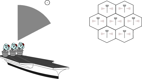
We illustrate our coexistence scenario in Figure 1 where the maritime MIMO radar is sharing interference channels with the cellular system. Considering this scenario, the received signal at the BS receiver can be written as
| (9) |
The goal of the MIMO radar is to map onto the null-space of in order to avoid interference to the BS, i.e., , so that has equation (7) instead of equation (9).
III-B Projection Matrix
In this section, we define the projection algorithm which projects radar signal onto the null space of interference channel . Assuming, the MIMO radar has channel state information of all interference channels, through feedback, in Mil2Mil or Mil2Com scenario, we can perform singular value decomposition (SVD) to find the null space and then construct a projector matrix. We proceed by first finding SVD of , i.e.,
| (10) |
Now, let us define
| (11) |
where and are the singular values of . Next, we define
| (12) |
where
| (13) |
Using above definitions we can now define our projection matrix, i.e.,
| (14) |
In order to show that is a valid projection matrix we prove two results on projection matrices below.
Property 1.
is a projection matrix if and only if .
Proof.
Let’s start by showing the ‘only if’ part. First, we show . Taking Harmition of equation (14) we have
| (15) |
Now, squaring equation (14) we have
| (16) |
where above equation follows from (since they are orthonormal matrices) and (by construction). From equations (15) and (16) it follows that . Next, we show is a projector by showing that if range (), then , i.e., for some , then
| (17) |
Moreover, null(), i.e.,
| (18) |
This concludes our proof.
∎
Property 2.
is an orthogonal projection matrix onto the null space of .
Proof.
Since , we can write
| (19) |
The above results follows from noting that by construction. ∎
In this paper, we are dealing with interference channels. Therefore, we need to select the interference channel which results in least degradation of radar waveform in a minimum norm sense, i.e.,
| (20) | ||||
| (21) |
Once we have selected our projection matrix it is straight forward to project radar signal onto the null space of interference channel via
| (22) |
The correlation matrix of our NSP waveform is given as
| (23) |
which is no longer identity and its rank depends upon the rank of the projection matrix.
III-C Spectrum Sharing and Projection Algorithms
The process of spectrum sharing by forming projection matrices and selecting interference channels is executed with the help of Algorithms (1) and (2). First, at each pulse repetition interval (PRI), the radar obtains ICSI of all interference channels. This information is sent to Algorithm (2) for the calculation of null spaces and formation of projection matrices. Algorithm (1) process projection matrices, received from Algorithm (2), to find the projection matrix which results in least degradation of radar waveform in a minimum norm sense. This step is followed by the projection of radar waveform onto the null space of the selected BS, i.e, the BS to the corresponding selected projection matrix, and waveform transmission.
IV Statistical Decision Test for Target Detection
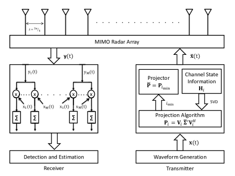
In this section, we develop a statistical decision test for target illuminated with the orthogonal radar waveforms and the NSP projected radar waveforms. The goal is to compare the performance of the two waveforms by looking at the test decision on whether the target is present or not in the range-Doppler cell of interest. We present a system-level architecture of the spectrum sharing radar in Figure 2. In our architecture, the transmitter performs the functions of waveform generation, channel selection, and projection; and the receiver performs the functions of signal detection and estimation.
For target detection and estimation, we proceed by constructing a hypothesis test where we seek to choose between two hypothesis: the null hypothesis which represents the case when the target is absent or the alternate hypothesis which represents the case when the target is present. The hypothesis for a single target model in equation (5) can be written as
| (24) |
Since, and are unknown, but deterministic, we use the generalize likelihood ratio test (GLRT). The advantage of using GLRT is that we can replace the unknown parameters with their maximum likelihood (ML) estimates. The ML estimate of and are found for various signal models, targets, and interference sources in [29, 31] when using orthogonal signals. In this paper, we consider a simpler model with one target and no interference sources in order to study the impact of NSP on target detection in a tractable manner. Therefore, we present a simpler derivation of ML estimation and GLRT.
We use Karhunen-Loève expansion for derivation of the log-likelihood function for estimating and . Let denote the space of the elements of and . Moreover, let , be an orthonormal basis function of satisfying
| (27) |
where is the Krönecker delta function. Then, the following series can be used to expand the processes, and , as
| (28) | ||||
| (29) | ||||
| (30) |
where , and are the coefficients in the Karhunen-Loève expansion of the considered processes obtained by taking the corresponding inner product with basis function . Thus, an equivalent discrete model of equation (25) can be obtained as
| (31) |
For white circular complex Gaussian processes, i.e, , the sequence is i.i.d. and . Thus, we can express the log-likelihood function as
| (32) |
Maximizing with respect to yields
| (33) |
where
| (34) | ||||
| (35) | ||||
| (36) | ||||
| (37) |
Note that, in equation (33), apart from the constant , the remaining summation goes to infinity. However, due to the non-contribution of higher order terms in the estimation of and the summation can be finite. Using the identity
| (38) |
for equations (35)-(37) can be written as
| (39) | ||||
| (40) | ||||
| (41) |
Using the definition of in equation (26), we can write the element of as
| (42) |
where
| (43) |
Similarly, we can write the element of as
| (44) |
Since, and are independent of the received signal, the sufficient statistic to calculate and is given by . Using equation (42)-(44) we can write the ML estimate in matrix-vector form as
| (45) |
Then, the GLRT for our hypothesis testing model in equation (24) is given as
| (46) |
where and are the probability density functions of the received signal under hypothesis and , respectively. Hence, the GLRT can be expressed as
| (47) |
The asymptotic statistics of for both the hypothesis is given by [32]
| (48) |
where
-
•
is the noncentral chi-squared distributions with two degrees of freedom,
-
•
is the central chi-squared distributions with two degrees of freedom,
-
•
and is the noncentrality parameter, which is given by
(49)
For the general signal model, we set according to a desired probability of false alarm , i.e.,
| (50) | ||||
| (51) |
where is the inverse central chi-squared distribution function with two degrees of freedom. The probability of detection is given by
| (52) | ||||
| (53) |
where is the noncentral chi-squared distribution function with two degrees of freedom and noncentrality parameter .
IV-A for Orthogonal Waveforms
For orthogonal waveforms , therefore, the GLRT can be expressed as
| (54) |
and the statistics of for this case is
| (55) |
where
| (56) |
We set according to a desired probability of false alarm , i.e.,
| (57) |
and then the probability of detection for orthogonal waveforms is given by
| (58) |
IV-B for NSP Waveforms
For spectrum sharing waveforms , therefore, the GLRT can be expressed as
| (59) |
and the statistics of for this case is
| (60) |
where
| (61) |
We set according to a desired probability of false alarm , i.e.,
| (62) |
and then the probability of detection for orthogonal waveforms is given by
| (63) |
V Numerical Results
In order to study the detection performance of spectrum sharing MIMO radars, we carry out Monte Carlo simulation using the radar parameters mentioned in Table II. At each run of Monte Carlo simulation we generate Rayleigh interference channels each with dimensions , calculate their null spaces and construct corresponding projection matrices using Algorithm (2), determine the best channel to perform projection of radar signal using Algorithm (1), transmit NSP signal, estimate parameters and from the received signal, and calculate the probability of detection for orthogonal and NSP waveforms.
| Parameters | Notations | Values |
|---|---|---|
| Radar/Communication System RF band | - | MHz |
| Radar antennas | 8, 4 | |
| Communication System Antennas | 2 | |
| Carrier frequency | 3.55 GHz | |
| Wavelength | 8.5 cm | |
| Inter-element antenna spacing | 6.42 cm | |
| Radial velocity | 2000 m/s | |
| Speed of light | 3 m/s | |
| Target distance from the radar | 500 Km | |
| Target angle | ||
| Doppler angular frequency | ||
| Two way propagation delay | ||
| Path loss |
V-A Performance of Algorithms (1) and (2)
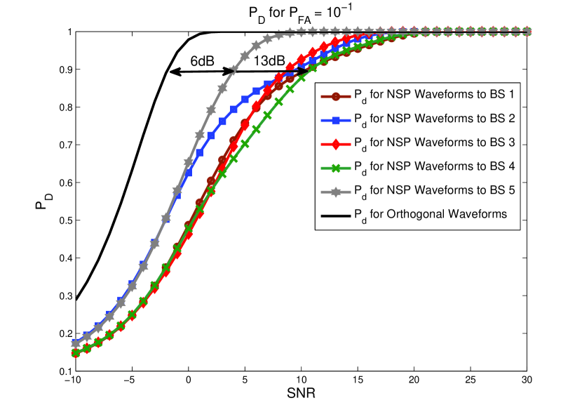
In Figure 3, we demonstrate the use of Algorithms (1) and (2) in improving target detection performance when multiple BSs are present in detection space of radar and the radar has to reliably detect target while not interfering with communication system of interest. As an example, we consider a scenario with five BSs and the radar has to select a projection channel which minimizes degradation in its waveform, thus, maximizing its probability of detection of the target.
In Figure 3(a), we consider the case when . We show detection results for five different NSP signals, i.e, radar waveform projected onto five different BSs. Note that, in order to achieve a detection probability of 90%, we need 6 dB to 13 dB more gain in SNR as compared to the orthogonal waveform, depending upon which channel we select. Using Algorithms (1) and (2) we can select interference channel that results in minimum degradation of radar waveform and results in enhanced target detection performance with the minimum additional gain in SNR required. For example, Algorithms (1) and (2) would select BS#5 because in this case NSP waveform requires least gain in SNR to achieve a detection probability of 90% as compared to other BSs.
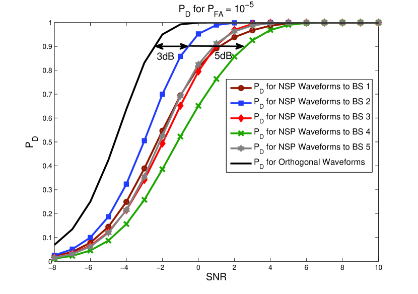
In Figure 3(b), we consider the case when . Similar to Figure 3(a) we show detection results for five different NSP signals but now MIMO radar has a larger array of antennas as compared to the previous case. In this case, in order to achieve a detection probability of 90%, we need 3 dB to 5 dB more gain in SNR as compared to the orthogonal waveform. As in the previous case, using Algorithms (1) and (2) we can select interference channel that results in minimum degradation of radar waveform and results in enhanced target detection performance with the minimum additional gain in SNR required. For example, Algorithms (1) and (2) would select BS#2 because in this case NSP waveform requires least gain in SNR to achieve a detection probability of 90% as compared to the other BSs.
The above two examples demonstrates the importance of Algorithms (1) and (2) in selecting interference channel for radar signal projection to maximize detection probability and minimize gain in SNR required as a result of NSP of radar waveforms for spectrum sharing.
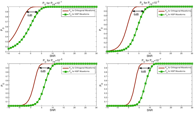
V-B Case 1:
In Figure 4, we plot the variations of probability of detection as a function of signal-to-noise ratio (SNR) for various values of probability of false alarm . Each sub-plot represents the for a fixed . We choose to evaluate against values of and when the interference channel has dimensions , i.e., the radar has antennas and the communication system has antennas, thus, we have a null space dimension of ‘’. When we compare the detection performance of two waveforms we note that in order to get a desired for a fixed we need more SNR for NSP than orthogonal waveforms. For example, say we desire , then according to Figure 4 we need 6 dB more gain in SNR for NSP waveform to get the same result produced by the orthogonal waveform.
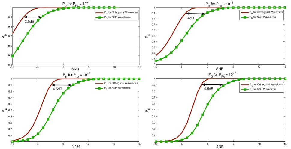
V-C Case 2:
In Figure 5, similar to Figure 4, we do an analysis of against the same values of but for interference channel having dimensions , i.e., now the radar has antennas and the communication system has antennas, thus, we have a null space dimension of ‘’. Similar to Case 1, when we compare the detection performance of two waveforms we note that in order to get a desired for a fixed we need more SNR for NSP than the orthogonal waveforms. For example, say we desire , then according to Figure 5 we need 3.5 to 4.5 dB more gain in SNR for the NSP waveform to get the same result produced by the orthogonal waveform.
V-D Comparison of Case 1 and Case 2
As expected, when SNR increases detection performance increases for both waveforms. However, when we compare the two waveforms at a fixed value of SNR, the orthogonal waveforms perform much better than the NSP waveform in detecting target. This is because our transmitted waveforms are no longer orthogonal and we lose the advantages promised by orthogonal waveforms when used in MIMO radars as discussed in Section II-F, but, we ensure zero interference to the BS of interest, thus, sharing radar spectrum at an increased cost of target detection in terms of SNR.
In Case 1, in order to achieve a desired for a fixed we need more SNR for NSP as compared to Case 2. This is because we are using more radar antennas, while the antennas at the BS remain fixed, in Case 2 which increases the dimension of the null space of the interference channel. This yields better detection performance even for NSP waveform. So, in order to mitigate the effect of NSP on radar performance one way is to employ a larger array at the radar transmitter.
VI Conclusion
In the future, radar RF spectrum will be shared with wireless communication systems to meet the growing bandwidth demands and mitigate the effects of spectrum congestion for commercial wireless services. In this paper, we analyzed a similar spectrum sharing scenario between radars and cellular systems. We proposed a spectrum sharing scenario in which a MIMO radar is sharing spectrum with a cellular system. We proposed algorithms for interference channel selection and projection of radar waveform onto the selected interference channel in order to mitigate interference to the selected BS. We evaluated the detection performance of spectrum sharing MIMO radars. We formulated the statistical detection problem for target detection and used generalized likelihood ratio test to decide about the presence of target when using orthogonal waveforms and null-space projected (NSP) waveforms. We showed that by using our spectrum sharing and projection algorithms the radar can maximize target detection probability and minimize additional gain in SNR required to detect the target. We showed that when using the NSP waveforms, the detection performance degrades as compared to the orthogonal waveforms and we need more SNR to detect reliably. Our results showed that, about 6 dB of gain in SNR is required when and 3.5 to 4.5 dB of gain in SNR is required when when NSP waveforms are used instead of orthogonal waveforms for spectrum sharing. Our analysis showed that this degradation in performance can be mitigated by using a larger array at the MIMO radar transmitter.
References
- [1] S. Haykin, “Cognitive radio: Brain-empowered wireless communications,” IEEE Journal on Selected Areas in Communications, vol. 23, pp. 201–220, Feb 2005.
- [2] T. Yucek and H. Arslan, “A survey of spectrum sensing algorithms for cognitive radio applications,” IEEE Communications Surveys Tutorials, vol. 11, pp. 116–130, First 2009.
- [3] R. Murty, R. Chandra, T. Moscibroda, and P. V. Bahl, “Senseless: A database-driven white spaces network,” IEEE Transactions on Mobile Computing, vol. 11, pp. 189–203, Feb. 2012.
- [4] Y. Zhao, L. Morales, J. Gaeddert, K. Bae, J.-S. Um, and J. Reed, “Applying radio environment maps to cognitive wireless regional area networks,” in 2nd IEEE International Symposium on New Frontiers in Dynamic Spectrum Access Networks (DySPAN), pp. 115–118, April 2007.
- [5] B. Gao, J. Park, and Y. Yang, “Uplink soft frequency reuse for self-coexistence of cognitive radio networks,” IEEE Transactions on Mobile Computing, vol. 13, pp. 1366–1378, June 2014.
- [6] Federal Communications Commission (FCC), “FCC proposes innovative small cell use in 3.5 GHz band.” Online: http://www.fcc.gov/document/fcc-proposes-innovative-small-cell-use-35-ghz-band, December 12, 2012.
- [7] Federal Communications Commission (FCC), “Connecting America: The national broadband plan.” Online, 2010.
- [8] The President s Council of Advisors on Science and Technology (PCAST), “Realizing the full potential of government-held spectrum to spur economic growth,” July 2012.
- [9] National Telecommunications and Information Administration (NTIA), “An assessment of the near-term viability of accommodating wireless broadband systems in the 1675-1710 MHz, 1755-1780 MHz, 3500-3650 MHz, 4200-4220 MHz, and 4380-4400 MHz bands (Fast Track Report).” Online, October 2010.
- [10] Federal Communications Commission (FCC), “In the matter of revision of parts 2 and 15 of the commission s rules to permit unlicensed national information infrastructure (U-NII) devices in the 5 GHz band.” MO&O, ET Docket No. 03-122, June 2006.
- [11] L. S. Wang, J. P. McGeehan, C. Williams, and A. Doufexi, “Application of cooperative sensing in radar-communications coexistence,” IET Communications, vol. 2, pp. 856–868, 2008.
- [12] S. S. Bhat, R. M. Narayanan, and M. Rangaswamy, “Bandwidth sharing and scheduling for multimodal radar with communications and tracking,” in IEEE Sensor Array and Multichannel Signal Processing Workshop, p. 233 236, 2012.
- [13] R. Saruthirathanaworakun, J. Peha, and L. Correia, “Performance of data services in cellular networks sharing spectrum with a single rotating radar,” in IEEE International Symposium on a World of Wireless, Mobile and Multimedia Networks (WoWMoM), pp. 1–6, 2012.
- [14] C. Rossler, E. Ertin, and R. Moses, “A software defined radar system for joint communication and sensing,” in IEEE Radar Conference (RADAR), pp. 1050–1055, May 2011.
- [15] R. Y. X. Li, Z. Zhang, and W. Cheng, “Research of constructing method of complete complementary sequence in integrated radar and communication,” in IEEE Conference on Signal Processing, vol. 3, p. 1729 1732, 2012.
- [16] C. Sturm and W. Wiesbeck, “Waveform design and signal processing aspects for fusion of wireless communications and radar sensing,” Proceedings of the IEEE, vol. 99, pp. 1236–1259, July 2011.
- [17] M. P. Fitz, T. R. Halford, I. Hossain, and S. W. Enserink, “Towards simultaneous radar and spectral sensing,” in IEEE International Symposium on Dynamic Spectrum Access Networks (DYSPAN), pp. 15–19, April 2014.
- [18] X. Chen, X. Wang, S. Xu, and J. Zhang, “A novel radar waveform compatible with communication,” in International Conference on Computational Problem-Solving (ICCP), p. 177 181, 2011.
- [19] A. Khawar, A. Abdel-Hadi, and T. C. Clancy, “Spectrum sharing between S-band radar and LTE cellular system: A spatial approach,” in 2014 IEEE International Symposium on Dynamic Spectrum Access Networks: SSPARC Workshop (IEEE DySPAN 2014 - SSPARC Workshop), (McLean, USA), Apr. 2014.
- [20] A. Khawar, A. Abdel-Hadi, and T. C. Clancy, “MIMO radar waveform design for coexistence with cellular systems,” in IEEE International Symposium on Dynamic Spectrum Access Networks: SSPARC Workshop (IEEE DySPAN 2014 - SSPARC Workshop), (McLean, USA), Apr. 2014.
- [21] M. Ghorbanzadeh, A. Abdelhadi, and C. Clancy, “A utility proportional fairness resource allocation in spectrally radar-coexistent cellular networks,” in Military Communications Conference (MILCOM), 2014.
- [22] A. Khawar, A. Abdelhadi, and T. C. Clancy, “On The Impact of Time-Varying Interference-Channel on the Spatial Approach of Spectrum Sharing between S-band Radar and Communication System,” in Military Communications Conference (MILCOM), 2014.
- [23] H. Shajaiah, A. Khawar, A. Abdel-Hadi, and T. C. Clancy, “Using resource allocation with carrier aggregation for spectrum sharing between radar and 4G-LTE cellular system,” in IEEE DySPAN, 2014.
- [24] F. Paisana, J. P. Miranda, N. Marchetti, and L. A. DaSilva, “Database-aided sensing for radar bands,” in IEEE International Symposium on Dynamic Spectrum Access Networks (DYSPAN), pp. 1–6, April 2014.
- [25] H. Deng and B. Himed, “Interference mitigation processing for spectrum-sharing between radar and wireless communications systems,” IEEE Transactions on Aerospace and Electronic Systems, vol. 49, no. 3, pp. 1911–1919, 2013.
- [26] A. M. Haimovich, R. S. Blum, and L. J. Cimini, “MIMO radar with widely separated antennas,” IEEE Signal Processing Magazine, vol. 25, no. 1, pp. 116–129, 2008.
- [27] J. Li and P. Stoica, “MIMO radar with colocated antennas,” IEEE Signal Processing Magazine, vol. 24, no. 5, pp. 106–114, 2007.
- [28] M. Skolnik, Radar Handbook. McGraw-Hill Professional, 3rd ed., 2008.
- [29] J. Li and P. Stoica, MIMO Radar Signal Processing. Wiley-IEEE Press, 2008.
- [30] D. Tse and P. Viswanath, Fundamentals of Wireless Communication. Cambridge University Press, 2005.
- [31] I. Bekkerman and J. Tabrikian, “Target detection and localization using mimo radars and sonars,” IEEE Transactions on Signal Processing, vol. 54, pp. 3873–3883, Oct 2006.
- [32] S. Kay, Fundamentals of Statistical Signal Processing: Detection Theory. Prentice Hall, 1998.