Spectral analysis of structure functions and their scaling exponents in forced isotropic turbulence

Abstract

The pseudospectral method, in conjunction with a new technique for obtaining scaling exponents $\zeta_{n}$ from the structure functions $S_{n}(r)$, is presented as an alternative to the extended self-similarity (ESS) method and the use of generalized structure functions. We propose plotting the ratio $|S_{n}(r)/S_{3}(r)|$ against the separation $r$ in accordance with a standard technique for analyzing experimental data. This method differs from the ESS technique, which plots $S_{n}(r)$ against $S_{3}(r)$, with the assumption $S_{3}(r)\sim r$. Using our method for the particular case of $S_{2}(r)$ we obtain the new result that the exponent $\zeta_{2}$ decreases as the Taylor-Reynolds number increases, with $\zeta_{2}\to 0.679\pm 0.013$ as $R_{\lambda}\to\infty$. This supports the idea of finite-viscosity corrections to the K41 prediction for $S_{2}$, and is the opposite of the result obtained by ESS. The pseudospectral method also permits the forcing to be taken into account exactly through the calculation of the energy input in real space from the work spectrum of the stirring forces.

I Introduction

In this paper we revisit an old, but unresolved, issue in turbulence: the controversy that continues to surround the Kolmogorov theory (or K41) Kolmogorov41a ; Kolmogorov41b . This controversy began with the publication in 1962 of Kolmogorov’s ‘refinement of previous hypotheses’ (K62), which gave a role to the intermittency of the dissipation rate Kolmogorov62 . From this beginning, the search for ‘intermittency corrections’ has grown into a veritable industry over the years: for a general discussion, see the book by Frisch Frisch95 and the review by Boffetta, Mazzino and Vulpiani Boffetta08 . The term ‘intermittency corrections’ is rather tendentious, as no relationship has ever been demonstrated between intermittency, which is a property of a single realization, and the ensemble-averaged energy fluxes which underlie K41, and it is now increasingly replaced by ‘anomalous exponents’. It has also been observed by Kraichnan Kraichnan74 , Saffman Saffman77 , Sreenivasan Sreenivasan99 and Qian Qian00 that the title of K62 is misleading. It in fact represents a profoundly different view of the underlying physics of turbulence, as compared to K41. For this reason alone it is important to resolve this controversy.

While this search has been a dominant theme in turbulence for many decades, at the same time there has been a small but significant number of theoretical papers exploring the effect of finite Reynolds numbers on the Kolmogorov exponents, such as the work by Effinger and Grossmann Effinger87 , Barenblatt and Chorin Barenblatt98a , Qian Qian00 , Gamard and George Gamard00 and Lundgren Lundgren02 . All of these papers have something to say; but the last one is perhaps the most compelling, as it appears to offer a rigorous proof of the validity of K41 in the limit of infinite Reynolds number. This is reinforced by the author’s comparison with the experimental results of Mydlarski and Warhaft Mydlarski96 .

The controversy surrounding K41 basically amounts to: ‘intermittency corrections’ versus ‘finite Reynolds number effects’. The former are expected to increase with increasing Reynolds number, the latter to decrease. In time, direct numerical simulation (DNS) should establish the nature of high-Reynolds-number asymptotics, and so decide between the two. In the meantime, one would like to find some way of extracting the ‘signature’ of this information from current simulations.

As is well known, one way of doing this is by Extended Self Similarity (ESS). The study of turbulence structure functions (e.g. see van Atta and Chen vanatta70 and Anselmet, Gagne, Hopfinger and Antonia Anselmet84 ) was transformed in the mid-1990s by the introduction of ESS by Benzi and co-workers Benzi93 ; Benzi95 . Their method of plotting results for $S_{n}(r)$ against $S_{3}(r)$, rather than against the separation $r$, showed extended regions of apparent scaling behavior even at low-to-moderate values of the Reynolds number, and was widely taken up by others e.g. Fukayama, Oyamada, Nakano, Gotoh and Yamamoto Fukayama00 , Stolovitzky, Sreenivasan and Juneja Stolovitzky93 , Meneveau Meneveau96 , Grossmann, Lohse and Rech Grossmann97 and Sain, Manu and Pandit Sain98 . A key feature of this work was the implication that corrections to the exponents of structure functions increase with increasing Reynolds number, which suggests that intermittency is the dominant effect. In the next section, we will explain ESS in more detail, in terms of how it relates to other ways of obtaining exponents.

II Structure functions, exponents and ESS

In this section we discuss the various ways in which exponents are defined and measured. The longitudinal structure functions are defined as

$$S_{n}(r)=\left\langle\delta u^{n}_{L}(r)\right\rangle\ ,$$ (1)

where the (longitudinal) velocity increment is given by

$$\delta u_{L}(r)=\Big{[}\bm{u}(\bm{x}+\bm{r},t)-\bm{u}(\bm{x},t)\Big{]}\cdot\bm{\hat{r}}\ .$$ (2)

Integration of the Kármán-Howarth equation (KHE) leads, in the limit of infinite Reynolds number, to the Kolmogorov ‘4/5’ law, $S_{3}(r)=-(4/5)\varepsilon r$. If the $S_{n}$, for $n\geq 4$, exhibit a range of power-law behavior, then; in general, and solely on dimensional grounds, the structure functions of order $n$ are expected to take the form

$$S_{n}(r)=C_{n}(\varepsilon r)^{n/3}\ .$$ (3)

Measurement of the structure functions has repeatedly found a deviation from the above dimensional prediction for the exponents. If the structure functions are taken to scale with exponents $\zeta_{n}$, thus:

$$S_{n}(r)\sim r^{\zeta_{n}}\ ,$$ (4)

then it has been found Anselmet84 ; Benzi95 that the difference $\Delta_{n}=\lvert n/3-\zeta_{n}\rvert$ is non-zero and increases with order $n$. Exponents $\zeta_{n}$ which differ from $n/3$ are often referred to as anomalous exponents Benzi95 .

In order to study the behavior of the exponents $\zeta_{n}$, it is usual to make a log-log plot of $S_{n}$ against $r$, and measure the local slope:

$$\zeta_{n}(r)=\frac{d\log{S_{n}(r)}}{d\log{r}}\ .$$ (5)

Following Fukayama et al. Fukayama00 , the presence of a plateau when any $\zeta_{n}(r)$ is plotted against $r$ indicates a constant exponent, and hence a scaling region. Yet, it is not until comparatively high Reynolds numbers are attained that such a plateau is found. Instead, as seen in Fig. 1 (symbols), even for the relatively large value of Reynolds number, $R_{\lambda}=177$, a scaling region cannot be identified. (We note that Grossmann et al. Grossmann97 have argued that a minimum value of $R_{\lambda}\sim 500$ is needed for satisfactory direct measurement of local scaling exponents.)

Figure 1: Comparison of our values of local-slope exponents $\zeta_{n}(r)$ (symbols) given in (5) with our values of the ESS exponents $\Sigma_{n}(r)$ (lines) as calculated from equation (8), divided by $n/3$ to show their relationship to K41 exponents. Results are given for $n=2,4,6$. Both sets of exponents were calculated from the real-space velocity field and are presented here for $R_{\lambda}=177$. The separation, $r$, has been scaled on the dissipation scale, $\eta=(\nu_{0}^{3}/\varepsilon)^{1/4}$.

The introduction of ESS relied on the fact that $S_{3}$ scales with $\zeta_{3}=1$ in the inertial range. Benzi et al. Benzi93 argued that if

$$S_{n}(r)\sim[S_{3}(r)]^{\zeta^{*}_{n}}\ ,\quad\textrm{with}\quad\zeta^{*}_{n}=\zeta_{n}/\zeta_{3}\ .$$ (6)

$\zeta^{*}_{n}$ should then be equivalent to $\zeta_{n}$ in the scaling region.

A practical difficulty led to a further step. The statistical convergence of odd-order structure functions is significantly slower than that for even-orders, due to the delicate balance of positive and negative values involved in the former Fukayama00 . To overcome this, generalized structure functions, where the velocity difference is replaced by its modulus, have been introduced Benzi93 (see also Stolovitzky93 ; Fukayama00 ),

$$G_{n}(r)=\left\langle\lvert\delta u_{L}(r)\rvert^{n}\right\rangle\sim r^{\zeta^{\prime}_{n}},$$ (7)

with scaling exponents $\zeta^{\prime}_{n}$. The fact that $S_{3}\sim r$ in the inertial range does not rigorously imply that $G_{3}\sim r$ in the same range. But, by plotting $G_{3}(r)$ against $\lvert S_{3}(r)\rvert$, Benzi et al. Benzi95 showed that, for $R_{\lambda}=225$ – 800, the third-order exponents satisfied $\zeta^{\prime}_{3}\simeq 1.006\zeta_{3}$. Hence, it is now generally assumed that $\zeta^{\prime}_{n}$ and $\zeta_{n}$ are equal (although, Fig. 2 in Belin, Tabeling and Willaime Belin96 implies some discrepancy at the largest length scales, and the authors note that the exponents $\zeta^{\prime}_{n}$ and $\zeta_{n}$ need not be the same). Thus, by extension, $G_{3}$ with $\zeta^{\prime}_{3}=1$, leads to

$$G_{n}(r)\sim[G_{3}(r)]^{\Sigma_{n}},\quad\textrm{with}\quad\Sigma_{n}=\zeta^{\prime}_{n}/\zeta^{\prime}_{3}\ .$$ (8)

Benzi et al. Benzi93 found that plotting their results on this basis gave a larger scaling region. This extended well into the dissipative lengthscales and allowed exponents to be more easily extracted from the data. Also, Grossmann et al. Grossmann97 state that the use of generalized structure functions is essential to take full advantage of ESS.

There is, however, an alternative to the use of generalized structure functions. This is the pseudospectral method. In using this for some of the present work, we followed the example of Qian Qian97 ; Qian99 , Tchoufag, Sagaut and Cambon Tchoufag12 and Bos, Chevillard, Scott and Rubinstein Bos12 , who obtained $S_{2}$ and $S_{3}$ from the energy and energy transfer spectra, respectively, by means of exact quadratures.

The organization of our own work in this paper is now as follows. We begin with a description of our DNS before illustrating ESS, using results from our own simulations, in section IV, where we show that our results for ESS agree closely with those of other investigations Benzi95 ; Fukayama00 . These particular results were obtained in the usual way by direct convolution sums, using a statistical ensemble, and the generalized structure functions. In section V we describe the theoretical basis for using the pseudospectral method Qian97 ; Qian99 ; Tchoufag12 ; Bos12 which includes a rigorous derivation of the forcing in the real-space energy balance equation. This is followed by the introduction of a new scaling exponent in section VI and a presentation of our numerical results for seven Taylor-scale Reynolds numbers spanning the range $101.3\leq R_{\lambda}\leq 435.2$.

III Numerical method

We used a pseudospectral DNS, with full dealiasing implemented by truncation of the velocity field according to the two-thirds rule Orszag71 . Time advancement for the viscous term was performed exactly using an integrating factor, while the non-linear term was stepped forward in time using Heun’s method Heun00 , which is a second-order predictor-corrector routine. Each simulation was started from a Gaussian-distributed random field with a specified energy spectrum, which followed $k^{4}$ for the low-$k$ modes. Measurements were taken after the simulations had reached a stationary state. The system was forced by negative damping, with the Fourier transform of the force $\bm{f}$ given by

$$\bm{f}(\bm{k},t) =(\varepsilon_{W}/2E_{f})\bm{u}(\bm{k},t)\quad\text{for}\quad 0<\lvert\bm{k}\rvert<k_{f};$$

$$=0\quad\textrm{otherwise},$$ (9)

where $\bm{u}(\bm{k},t)$ is the instantaneous velocity field (in wavenumber space). The highest forced wavenumber, $k_{f}$, was chosen to be $k_{f}=2.5k_{min}$, where $k_{min}=2\pi/L_{box}=1$ is the lowest resolved wavenumber. As $E_{f}$ was the total energy contained in the forcing band, this ensured that the energy injection rate was $\varepsilon_{W}=\textrm{constant}$. It is worth noting that any method of energy injection employed in the numerical simulation of isotropic turbulence is not experimentally realizable. The present method of negative damping has also been used in other investigations Jimenez93 ; Yamazaki02 ; Kaneda03 ; Kaneda06 , albeit not necessarily such that $\varepsilon_{W}$ is maintained constant (although note the theoretical analysis of this type of forcing by Doering and Petrov Doering05 ). Also, note that the correlation between the force and the velocity is restricted to the very lowest wavenumbers.

For each Reynolds number studied, we used the same initial spectrum and input rate $\varepsilon_{W}$. The only initial condition changed was the value assigned to the (kinematic) viscosity. Once the initial transient had passed, the velocity field was sampled every half a large-eddy turnover time, $\tau=L/U$, where $L$ denotes the average integral scale and $U$ the rms velocity. The ensemble populated with these sampled realizations was used, in conjunction with the usual shell averaging, to calculate statistics. Simulations were run using lattices of size $128^{3},\ 256^{3},\ 512^{3},\ 1024^{3}$ and $2048^{3}$, with corresponding Reynolds numbers ranging from $R_{\lambda}=41.8$ up to $435.2$. The smallest wavenumber was $k_{\text{min}}=2\pi/L_{\text{box}}=1$ in all simulations, while the maximum wavenumber satisfied $k_{\text{max}}\eta\geqslant 1.30$ for all runs except one which satisfied $k_{\text{max}}\eta\geqslant 1.01$, where $\eta$ is the Kolmogorov dissipation lengthscale. The integral scale, $L$, was found to lie between $0.23L_{\text{box}}$ and $0.17L_{\text{box}}$. It can be seen in Figure 2 of McComb, Hunter and Johnston McComb01a that a small-scale resolution of $k_{max}\eta>1.6$ is desirable in order to capture the relevant dissipative physics. Evidently, this would restrict the attainable Reynolds number of the simulated flow, and the reference suggests that $k_{max}\eta\geqslant 1.3$ would still be acceptable (containing $\sim 99.5\%$ of dissipative dynamics Yoffe12 ). In contrast, at $k_{max}\eta\simeq 1$ a non-negligible part of dissipation is not taken into account. Most high resolution DNSs of isotropic turbulence try to attain Reynolds numbers as high possible and thus opt for minimal resolution requirements. In this paper the simulations have been conducted following a more conservative approach, where the emphasis has been put on higher resolution, thus necessarily compromising to some extent on Reynolds number. Large-scale resolution has only relatively recently received attention in the literature. As mentioned above, the largest scales of the flow are smaller than a quarter of the simulation box size. Details of the individual runs are summarized in Table 1.

Our simulations have been well validated by means of extensive and detailed comparison with the results of other investigations. Further details of the performance of our code including verification of isotropy may be found in the thesis by Yoffe Yoffe12 , along with values for the Kolmogorov constant and velocity-derivative skewness; and a direct comparison with the freely-available pseudospectral code hit3d Schumakov07 ; Schumakov08 . Furthermore our data reproduces the characteristic behavior for the plot of the dimensionless dissipation rate $C_{\varepsilon}$ against $R_{\lambda}$ McComb14a , and agree closely with other representative results in the literature, such as the work by Wang, Chen, Brasseur and Wyngaard Wang96 , Cao, Chen and Doolen Cao99 , Gotoh, Fukayama and Nakano Gotoh02 , Kaneda, Ishihara, Yokokawa, Itakura and Uno Kaneda03 , Donzis, Sreenivasan and Yeung Donzis05 and Yeung, Donzis and Sreenivasan Yeung12 , although there are some differences in forcing methods.

$R_{\lambda}$	$\nu_{0}$	$N$	$\varepsilon$	$U$	$L/L_{\text{box}}$	$k_{\text{max}}\eta$	$M$
42.5	0.01	128	0.094	0.581	0.23	2.34	101
64.2	0.005	128	0.099	0.607	0.21	1.37	101
101.3	0.002	256	0.099	0.607	0.19	1.41	101
113.3	0.0018	256	0.100	0.626	0.20	1.31
176.9	0.00072	512	0.102	0.626	0.19	1.31	15
203.7	0.0005	512	0.099	0.608	0.18	1.01
217.0	0.0005	1024	0.100	0.630	0.19	2.02
276.2	0.0003	1024	0.100	0.626	0.18	1.38
335.2	0.0002	1024	0.102	0.626	0.18	1.01
435.2	0.00011	2048	0.102	0.614	0.17	1.30

Table 1: A summary of the main parameters of our numerical simulations. The values quoted for the dissipation rate $\varepsilon$, the rms velocity $U$ and the integral scale $L$ are ensemble- and shell-averaged mean values, where the ensembles have been populated with snapshots of the steady-state velocity field taken every half large eddy turnover time. $M$ counts individual realizations used to calulate ESS exponents for those runs for which the ESS method has been performed, not the size of the ensemble used for calculating statistics.

IV Real-space calculation of the structure functions and ESS

In order to calculate the structure functions in real space, we calculate the longitudinal correlation of one lattice site with all other sites

$$S_{n}(r)=\frac{1}{3N^{3}}\sum_{\bm{x}}\bigg{[}\Big{(}u_{x}(\bm{x}+r\bm{e}_{x})-u_{x}(\bm{x})\Big{)}^{n}+\Big{(}u_{y}(\bm{x}+r\bm{e}_{y})-u_{y}(\bm{x})\Big{)}^{n}+\Big{(}u_{z}(\bm{x}+r\bm{e}_{z})-u_{z}(\bm{x})\Big{)}^{n}\bigg{]}\ ,$$ (10)

for each realization. The results are subsequently ensemble-averaged over many realizations.

Figure 2 shows the calculated standard local slopes for four different Reynolds numbers $R_{\lambda}=42$, 64, 101 and 177. A plateau would indicate a constant exponent, that is a scaling region, but the figure does not show the formation of plateaux for these Reynolds numbers, implying that there is no scaling region.

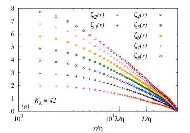
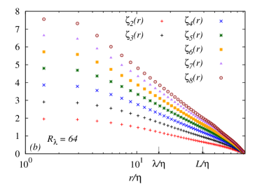
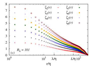
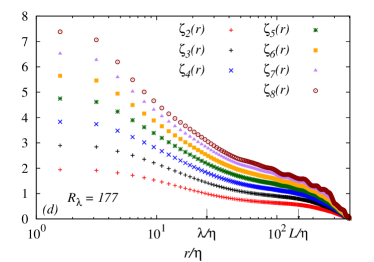
Figure 2: (Color online) The local slopes $\zeta_{n}(r)$ of the structure functions $S_{n}(r)$ for $n=2,\cdots,8$ from our DNS. The slopes are calculated using the structure functions evaluated in real space for Reynolds numbers $R_{\lambda}=42$, 64, 101 and 177. Note the absence of a scaling region in all cases.

If, in contrast the generalized structure functions are used to evaluate the local slopes $\Sigma_{n}$ as defined in (8), scaling regions are obtained and thus the ESS scaling exponents can be measured. As shown in Fig. 3, extended plateaux for each order of generalized structure function are observed, which reach well into the dissipation scales where we do not expect power-law behavior. Since $S_{n}\sim r^{n}$ as $r\to 0$, we note that $\Sigma_{n}(r)\to n/3$ as $r\to 0$. It should be borne in mind that this K41-type behavior is an artefact of ESS, as has been pointed out before Benzi95 ; Barenblatt99 ; Benzi99 . ESS exponents obtained from our calculations are shown to be consistent with relevant results from the literature in Table 2.

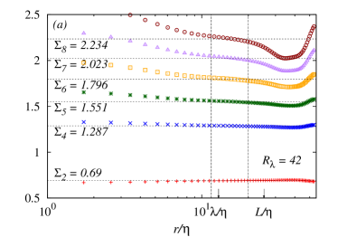
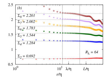
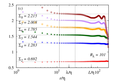
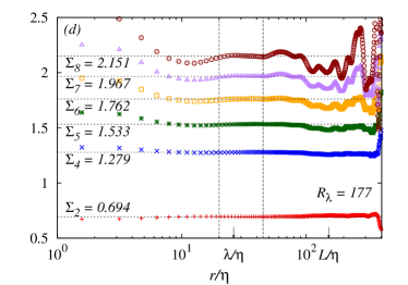
Figure 3: (Color online) The same results as in Fig. 2 evaluated using the ESS method for structure functions calculated in real space. The vertical lines indicate the scaling region used to evaluate the scaling exponent, $\Sigma_{n}$.

$R_{\lambda}$	$\Sigma_{2}$	$\Sigma_{4}$	$\Sigma_{5}$	$\Sigma_{6}$	$\Sigma_{7}$	$\Sigma_{8}$	Source
	0.667	1.333	1.667	2.000	2.333	2.667	K41 theory
42.5	0.690	1.287	1.551	1.796	2.023	2.234	Our DNS, $\Sigma_{n}$
64.2	0.692	1.284	1.544	1.783	2.002	2.201
101.3	0.692	1.283	1.544	1.785	2.008	2.215
176.9	0.694	1.279	1.533	1.762	1.967	2.151
70	0.690	1.288	1.555	1.804	2.037	2.254	DNS Fukayama00 , $\Sigma_{n}$
125	0.692	1.284	1.546	1.788	2.011	2.217
381	0.709	1.30	1.56	1.79	1.99	2.18	DNS Gotoh02 , $\zeta_{n}$
460	0.701	1.29	1.54	1.77	1.98	2.17
800	0.70	1.28	1.54	1.78	2.00	2.23	Exp. Benzi95 , $\Sigma_{n}$

Table 2: Measurement of the scaling exponents from our DNS data using ESS. For purposes of comparison, we also show the values predicted from dimensional analysis (referred to as ‘K41 theory’), along with results from Fukayama et al. Fukayama00 , Gotoh et al. Gotoh02 and Benzi et al. Benzi95 .

V Spectral methods

The use of spectral methods to calculate the structure functions is known in the literature through the work by Bos et al. Bos12 , Tchoufag et al. Tchoufag12 and Qian Qian97 ; Qian99 . We will now briefly explain the reason for doing it this way.

Since the calculation of correlation and structure functions in real space requires a convolution in which the correlation of each site with every other (longitudinal) site needs to be measured, moving to large lattice sizes in order to reach larger Reynolds numbers results in a significant increase in computational workload. In addition, the number of realizations required to generate the ensemble takes both longer to produce and occupies substantially more storage space. In order to reach higher Reynolds numbers we have therefore used spectral expressions for the correlation and structure functions. Real-space quantities are then calculated by Fourier-transforming the appropriate spectral density. For example, the two-point correlation tensor may be found using

$$C_{\alpha\beta}(\bm{r})=\int d^{3}k\ \left\langle u_{\alpha}(\bm{k})u^{*}_{\beta}(\bm{k})\right\rangle\ e^{i\bm{k}\cdot\bm{x}}\ .$$ (11)

The assumption of isotropy then allows the transformation for the calculation of the isotropic correlation function to be reduced to

$$C(r)=\tfrac{1}{2}C_{\alpha\alpha}(\bm{r})=\int dk\ E(k)\frac{\sin{kr}}{kr}\ .$$ (12)

The real space correlation tensor $C_{\alpha\beta}(\bm{r})$, when written as a spatial average instead of an ensemble average (assuming ergodicity, as is the usual practice), is a convolution

$$C_{\alpha\beta}(\bm{r})=\lim_{V\to\infty}\frac{1}{V}\int_{V}d\bm{x}\ u_{\alpha}(\bm{x})u_{\beta}(\bm{x}+\bm{r})\ ,$$ (13)

of the velocity components $u_{\alpha}$ and $u_{\beta}$. In a similar manner to the standard pseudospectral DNS technique, that is switching to real space in order to calculate the non-linear term and to avoid the convolution in Fourier space Yoffe12 , this approach replaces the convolution in real space with a Fourier transform of local Fourier-space spectra. Furthermore, the shell-averaged spectra require substantially less in the way of storage and processing capabilities than real-space ensembles.

The derivations of the spectral representation of the second- and third-order structure functions are given in Appendix A, leading to

$$S_{2}(r)=4\int_{0}^{\infty}dk\ E(k)a(kr)\ ,$$ (14)

and

$$S_{3}(r)=6C_{LL,L}(r)=12\int_{0}^{\infty}dk\ \frac{T(k)}{k^{2}}\ \frac{\partial a(kr)}{\partial r}\ ,$$ (15)

where

$$a(x)=\frac{1}{3}-\frac{\sin{x}-x\cos{x}}{x^{3}}\ ,$$ (16)

in agreement with Bos et al. Bos12 . The local slopes $\zeta_{n}$ can now be found by taking derivatives of the spectral forms for the structure functions, as shown in further detail in Appendix A.

The spectral approach has the consequence that we are now evaluating the conventional structure functions $S_{n}(r)$, rather than the generalized structure functions, $G_{n}(r)$, as commonly used (including by us) for ESS. Before proceeding to the calculation of the scaling exponents, we will now discuss the effects of finite forcing and the calculation of viscous corrections to the second- and third-order structure functions, and subsequently validate the pseudospectral approach by comparing results for the spectrally obtained second- and third-order structure functions to corresponding real-space results.

V.1 Effects of finite forcing on the structure functions

The pseudospectral method can also be used to calculate the corrections due to finite forcing on the structure functions. The second- and third-order structure functions are related by energy conservation, that is in real space by the Kármán-Howarth equation

$$-\frac{3}{2}\frac{\partial U^{2}}{\partial t}=-\frac{3}{4}\frac{\partial S_{2}}{\partial t}-\frac{1}{4r^{4}}\frac{\partial}{\partial r}\Big{(}r^{4}S_{3}\Big{)}+\frac{3\nu_{0}}{2r^{4}}\frac{\partial}{\partial r}\left(r^{4}\frac{\partial S_{2}}{\partial r}\right)\ ,$$ (17)

where $(3/2)\partial U^{2}/\partial t=\partial E/\partial t=-\varepsilon_{D}$, with $\varepsilon_{D}$ denoting the decay rate. For decaying turbulence the decay rate equals the dissipation rate $\varepsilon$, that is $\varepsilon_{D}=\varepsilon$. For stationary turbulence $\varepsilon_{D}=0$, and the dissipation rate then has to be equal to the energy input rate, that is $\varepsilon=\varepsilon_{W}$, where $\varepsilon_{W}$ denotes the energy input rate, and the time-dependent $S_{2}$ term vanishes. There is, however, a further complication. Replacing the dissipation rate $\varepsilon$ with the energy input rate $\varepsilon_{W}$, we see that the dissipation rate is acting as an input. In the K41 theory, we have an equivalence between the inertial transfer, dissipation, and input rates, in the infinite Reynolds number limit. However, in using $\varepsilon$ ($=\varepsilon_{W}$) as the input, it has been implicitly assumed that the forcing does not depend on the scale $r$. This is in general not the case, and as such some method for accounting for the effects of (finite) forcing (i.e. $Re<\infty$) must be introduced. Various proposals have been put forward, mainly through the inclusion of corrections to the KHE. These are discussed in Appendix B. An alternative treatment containing the exact energy input is given in the following section.

V.1.1 The KHE derived from the Fourier space energy balance

Instead of including a correction term in the KHE for forced turbulence, the effect of finite forcing can be calculated exactly using the spectral approach. We begin with the energy balance equation in spectral space (nowadays referred to as the Lin equation Sagaut08 ; McComb14a )

$$\frac{\partial E(k,t)}{\partial t}=T(k,t)-2\nu_{0}k^{2}E(k,t)+W(k,t)\ ,$$ (18)

where $W(k,t)$ is the work spectrum of the stirring forces and thus contains the relevant information about the forcing. In order to obtain the energy balance equation in real space including the effects of (finite) forcing, we assume isotropy, take the Fourier transform of the Lin equation and use the definitions of the structure functions $S_{2}$ and $S_{3}$ in order to obtain the energy balance equation in real space (the KHE) relating $S_{2}$ and $S_{3}$

$$\frac{\partial U^{2}}{\partial t}-\frac{1}{2}\frac{\partial S_{2}(r)}{\partial t}=\frac{1}{6r^{4}}\frac{\partial}{\partial r}\Big{(}r^{4}S_{3}(r)\Big{)}-\frac{\nu_{0}}{r^{4}}\frac{\partial}{\partial r}\left(r^{4}\frac{\partial S_{2}(r)}{\partial r}\right)+\frac{2}{3}I(r,t)\ ,$$ (19)

where the input term $I(r,t)$ is defined as

$$I(r,t)=\frac{3}{r^{3}}\int_{0}^{r}dy\ y^{2}W(y,t)\ ,$$ (20)

and $W(y,t)$ is the (three-dimensional) Fourier transform of the work spectrum $W(k,t)$. A detailed derivation of this equation from the Lin equation (18) can be found in Appendix C.

In order to write (19) in terms of energy loss, we multiply by $-3/2$ on both sides and obtain

$$\varepsilon_{D}=-\frac{3}{4}\frac{\partial S_{2}(r)}{\partial t}-\frac{1}{4r^{4}}\frac{\partial}{\partial r}\Big{(}r^{4}S_{3}(r)\Big{)}+\frac{3\nu_{0}}{2r^{4}}\frac{\partial}{\partial r}\left(r^{4}\frac{\partial S_{2}(r)}{\partial r}\right)-I(r,t)\ .$$ (21)

This is now the general form of the KHE including the effects of general, unspecified forcing. For the case of free decay, $\varepsilon_{D}=\varepsilon$ and the input term $I(r,t)=0$, which leads to the well-known KHE for free decay. On the other hand, for the stationary case $\varepsilon_{D}=0$, $\partial S_{2}/\partial t=0$ and the input term is independent of time $I(r,t)=I(r)$, thus

$$I(r)=-\frac{1}{4r^{4}}\frac{\partial}{\partial r}\Big{(}r^{4}S_{3}(r)\Big{)}+\frac{3\nu_{0}}{2r^{4}}\frac{\partial}{\partial r}\left(r^{4}\frac{\partial S_{2}(r)}{\partial r}\right)\ .$$ (22)

This derivation shows that the dissipation rate should not be present in the KHE for stationary turbulence with finite forcing. Only for the limit of $\delta(\bm{k})$-forcing do we obtain $I(r)=\varepsilon_{W}=\varepsilon$ and hence recover the dissipation rate as an input term.

In contrast to previous attempts to include the effects of forcing into the KHE, we do not approximate the work term. Instead, we use full information of this term as supplied by the work spectrum. In this way an explicit form for the actual energy input by the stirring forces can be calculated, as we shall now show. By integrating (22) with respect to $r$ one obtains

$$S_{3}(r)=X(r)+6\nu_{0}\frac{\partial S_{2}}{\partial r}\ ,$$ (23)

with the input due to finite forcing

$$X(r)=-\frac{4}{r^{4}}\int_{0}^{r}dy\ y^{4}I(y)$$ (24)

evaluated using the spectral method

$$X(r)=-12r\int_{0}^{\infty}dk\ W(k)\ \left[\frac{3\sin{kr}-3kr\cos{kr}-(kr)^{2}\sin{kr}}{(kr)^{5}}\right]\ .$$ (25)

Note that $X(r)$ is not a correction to K41, as used in previous studies. Instead, it replaces the erroneous use of the dissipation rate and contains all the information of the energy input at all scales. In the limit of $\delta(\bm{k})$-forcing, $I(y)=\varepsilon_{W}=\varepsilon$, such that $X(r)=-4\varepsilon r/5$, giving K41 in the infinite Reynolds number limit.

V.2 Real-space versus spectral structure functions

Results from pseudospectral calculations of the structure functions were compared to real space ensemble averaged results for $R_{\lambda}=101$ and $R_{\lambda}=177$. As can be seen in Fig. 4, agreement for $S_{2}(r)$ is very good for all $r$. For $S_{3}(r)$ we observe good agreement for small $r$, but the curves diverge at large $r$. This could be due to DNS data being periodic in $L_{\text{box}}=2\pi$. Since $S_{3}(r)$ is an odd function of $r$, it must go to zero in the center of the domain. The pseudospectral method, however, involves a (weighted) superposition of damped oscillating functions which does not necessarily require that $S_{3}(L_{\text{box}}/2)=0$. Figure 5 shows the compensated second- and third-order structure function calculated from real-space ensembles for the Taylor-scale Reynolds number range $43\leqslant R_{\lambda}\leqslant 177$. This may be compared to figure 3(b) in the paper by Ishihara, Gotoh and Kaneda Ishihara09 .

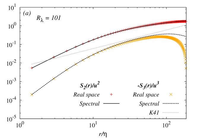
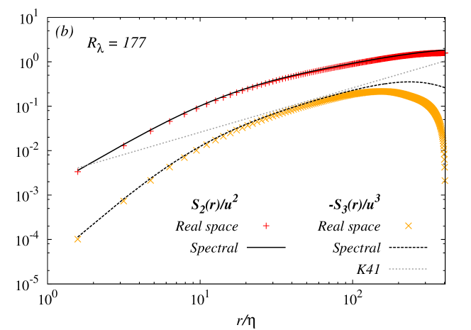
Figure 4: (Color online) Comparison of second- and third-order (scaled) structure functions calculated from the real-space ensembles and from energy and transfer spectra for two different Reynolds numbers. The agreement for $S_{2}$ is good at all scales, while for $S_{3}$ the results from real-space and spectral space calculations diverge at the large scales.

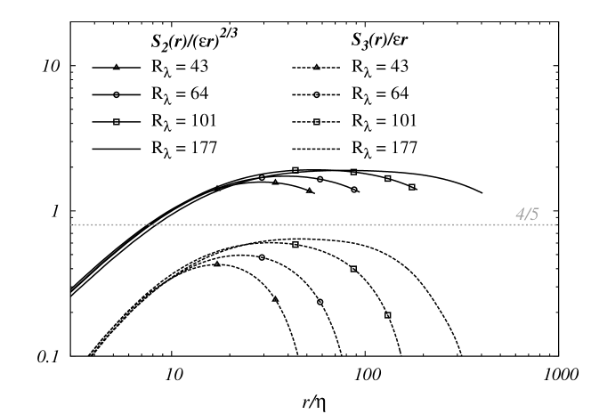
Figure 5: Second- and third-order (scaled) structure functions, calculated from the real-space ensembles. This figure should be compared to Fig. 6. The comparison shows how the real-space results can be extended to higher Reynolds numbers using the spectral method.

V.3 Spectral calculation from DNS

The pseudospectral method was used to calculate structure functions for $R_{\lambda}=101$, $113$ and also for the higher Reynolds number range $177\leqslant R_{\lambda}\leqslant 435$, which can be seen in Fig. 6, where the arrows indicate the direction of increasing Reynolds number. The lower horizontal dotted line in the picture indicates K41 scaling for the third-order structure function, while the upper horizontal line indicates our measured value $C_{K,S_{2}}=2.07$ for the prefactor $C_{K,S_{2}}$ of the second-order structure function. The prefactor $C_{K,S_{2}}$ is related to the prefactor $C_{K,E_{LL}}$ of the longitudinal energy spectrum $E_{LL}(k)$ by $C_{K,S_{2}}=4.02C_{K,E_{LL}}$ Monin75 , which has been measured by Sreenivasan Sreenivasan95 to be $C_{K,E_{LL}}=0.53\pm 0.055$. This results in $C_{K,S_{2}}=2.13\pm 0.22$, compared to our measured value of $C_{K,S_{2}}=2.07$. Comparison of Figs. 5 and 6 shows how the spectrally calculated results for the second- and third-order structure functions extend the real-space results to higher Reynolds numbers.

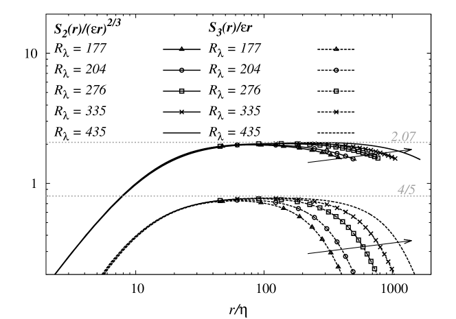
Figure 6: Compensated second- and third-order (scaled) structure functions, calculated from energy and transfer spectra. The horizontal lines indicate K41 scaling, where the upper horizontal line indicates our measured value $C_{K,S_{2}}=2.07$ for the prefactor $C_{K,S_{2}}$ of the second-order structure function. The arrows indicate the direction of increasing Reynolds number, and one observes the formation of longer plateaux for both $S_{2}$ and $S_{3}$ with increasing Reynolds number indicating an approach to K41 scaling.

The viscous correction to the ‘four-fifths’-law and to the exact input contribution $X(r)$ calculated by the spectral method are shown in Fig. 7 and Fig. 8, respectively, with the third-order structure function plotted for comparison. This is presented for our highest resolved simulation at $R_{\lambda}=435.2$. Together with the viscous correction, the input $X(r)$ given in (25) can be seen to account for differences between the third-order structure function and the ‘four-fifths’-law at all scales, as can be seen in Fig. 8. In contrast, Fig. 7 shows that the viscous correction alone only accounts for the difference between DNS data for the third-order structure function and K41 at the small scales, as expected, since at scales much smaller than the forcing scale the system becomes insensitive to the details of the (large-scale) forcing.

Figure 7: Evaluation of the viscous correction to the ‘four-fifths’-law for the third-order structure function using the spectral method, with $R_{\lambda}=435.2$. The correction can be seen to account for the difference between the ‘four-fifths’-law and DNS data at small scales.

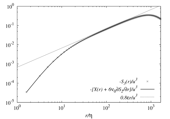
Figure 8: Evaluation of the viscous correction to the input $X(r)$ (in place of the ‘four-fifths’-law) for the third-order structure function. Calculations were performed using the spectral method, with $R_{\lambda}=435.2$. The contributions can be seen to account for the differences between the ‘four-fifths’-law and DNS data at all scales.

VI A new scaling exponent

We now arrive at our proposal to introduce a new local-scaling exponent $\Gamma_{n}$, which can be used to determine the $\zeta_{n}$. We work with $S_{n}(r)$ and consider the quantity $\lvert S_{n}(r)/S_{3}(r)\rvert$. In this procedure, the exponent $\Gamma_{n}$ is defined by

$$\left\lvert\frac{S_{n}(r)}{S_{3}(r)}\right\rvert\sim r^{\Gamma_{n}}\ ,\qquad\text{where}\qquad\Gamma_{n}=\zeta_{n}-\zeta_{3}\ .$$ (26)

The definition of $\Gamma_{n}$ is motivated by a long-established technique in experimental physics, where the effective experimental error can be reduced by plotting the ratio of two dependent variables: see e.g. Chapter 3 in the well-known book by Bevington and Robinson on data analysis Bevington03 . Of course this does not work in all cases, but only where the quantities are positively correlated, and we have verified that this is the case for $S_{2}$ and $\lvert S_{3}\rvert$.

The error in the measurement of the $n^{th}$-order structure function can be expressed as

$$S_{n}(r)=\Big{[}1+\epsilon_{n}(r)+O(\epsilon_{n}^{2})\Big{]}\overline{S}_{n}(r)\ ,$$ (27)

where $\overline{S}_{n}(r)$ is the ‘true’ value and $\epsilon_{n}(r)$ a measurement of the systematic error and considered small. Hence if $\epsilon_{n}(r)\sim\epsilon(r)$, then the ratio $\left\lvert\frac{S_{n}(r)}{S_{3}(r)}\right\rvert$ has an error proportional to the second-order of a small quantity,

$$\frac{S_{n}(r)}{S_{3}(r)}=\frac{\overline{S}_{n}(r)}{\overline{S}_{3}(r)}\Big{[}1-\epsilon^{2}(r)+O(\epsilon^{3})\Big{]}\ .$$ (28)

For illustration purposes we assumed here that $S_{n}$ and $S_{3}$ were perfectly correlated, note that for imperfect correlation there is still a reduction in error. The local slope now is found by considering $\Gamma_{2}(r)=\zeta_{2}(r)-\zeta_{3}(r)$. By once again assuming that $\zeta_{3}(r)=1$, the local slope for the second-order structure function is found as $\Gamma_{2}(r)+1=\zeta_{2}(r)$.

VI.1 Scaling exponents from spectra

The new scaling exponent $\Gamma_{n}$, based on the conventional (as opposed to the generalized) structure functions $S_{n}(r)$, is compatible with spectral methods and has been tested for the case $n=2$ in Fig. 9. The dimensionless quantity $U\lvert S_{2}(r)/S_{3}(r)\rvert$, where $U$ is the rms velocity, is plotted against $r/\eta$, for three values of $R_{\lambda}$. Note that, since K41 predicts $\Gamma_{2}=-1/3$, we have plotted a compensated form, in which we multiply the ratio by $(r/\eta)^{1/3}$, such that K41 scaling would correspond to a plateau. From the figure, we can see a trend towards K41 scaling as the Reynolds number is increased.

Figure 9: The compensated ratio $(r/\eta)^{1/3}U\lvert S_{2}(r)/S_{3}(r)\rvert$ plotted against $r$ and scaled on the dissipation scale, $\eta$. K41 scaling would correspond to a plateau. Arrows indicate $\lambda/\eta$, while the vertical dotted lines show the region used to fit each exponent. Note that the measured compensated slopes become flatter with increasing Reynolds number, pointing towards the deviation from Kolmogorov scaling being a finite Reynolds number effect.

Note that this figure also illustrates the ranges used to find values for our new exponent $\Gamma_{2}$, for the following cases. $\Gamma_{2}$ was fitted to the ranges $\lambda<r<c\lambda$, with $c=2.0,2.5,2.6$, and 2.7 for $R_{\lambda}=101,217,276$ and 435, respectively.

Figure 10 summarizes the comparison between our results for our new method of determining the second-order exponent and those based on ESS (our own and others Benzi95 ; Fukayama00 ) or on direct measurement Gotoh02 , in terms of their overall dependence on the Taylor-Reynolds number. In order to establish the form of the dependence of the exponents on Reynolds number, we fitted curves to the data points using the nonlinear-least-squares Marquardt-Levenberg algorithm, with the error quoted being one standard error. Using the data obtained from our new method, we fitted a curve $\Gamma_{2}+1=A+BR_{\lambda}^{p}$, to find the asymptotic value $A=0.679\pm 0.013$, which is consistent with the deviations from K41 scaling being finite Reynolds number effects. In order to compare this result with results obtained by the ESS method, we fitted the curve $\Sigma_{2}=C+DR_{\lambda}^{q}$ to our own data plus that of Fukayama et al. Fukayama00 . Evidently the two fitted curves show very different trends, with results for $\Sigma_{2}$ increasing with increasing Reynolds number, whereas $\zeta_{2}=\Gamma_{2}+1$ decreases and approaches 2/3 (within one standard error) as $R_{\lambda}$ increases.

It should be emphasized that with both methods, that is ESS and our new method, it is necessary to take $\zeta_{3}=1$ in the inertial range, in order to obtain the inertial-range value of either $\Sigma_{2}=\zeta_{2}$ (by ESS) or $\Gamma_{2}=\zeta_{2}-1$ (our new method). For this reason, we plot $\Gamma_{2}+1$, rather than $\Gamma_{2}$ in Fig. 10. An obvious difference between our proposed method and ESS is apparent as $r\to 0$. This is readily understood in terms of the regularity condition for the velocity field, which leads to $S_{n}(r)\sim r^{n}$ as $r\to 0$ Stolovitzky93 ; Sirovich94 . This yields $\Gamma_{n}(r)+1\to n-2$, whereas ESS gives $\Sigma_{n}(r)\to n/3$.

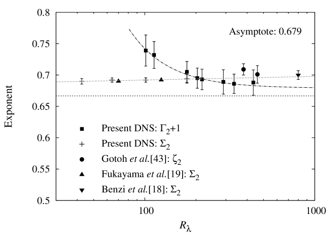
Figure 10: Dependence of our new exponent $\zeta_{2}=\Gamma_{2}+1$ on Reynolds number, compared to measured ESS exponents denoted by $\Sigma_{2}$ from Fukayama et al. Fukayama00 , Benzi et al. Benzi95 and our DNS, as well as results for $\zeta_{2}$ by Gotoh et al. Gotoh02 . The horizontal line indicates the K41 value of 2/3. The dash-dot line indicates the fit to $\Gamma_{2}+1$, while the dashed line shows a fit to $\Sigma_{2}$ using our results and those of Fukayama et al. Fukayama00 .

In this context it may be of interest to briefly discuss the experimental results of Mydlarski and Warhaft Mydlarski96 , who measured the exponent of the longitudinal energy spectrum for a range of Taylor-Reynolds numbers from $R_{\lambda}=50$ to $R_{\lambda}=473$, which is similar to the range of Taylor-Reynolds numbers studied in the present paper. The authors found the inertial-range exponent $\alpha$ of the longitudinal energy spectrum $E_{LL}(k)$ to depend on $R_{\lambda}$ in the following way

$$\alpha=-\frac{5}{3}\left(1+3.15R_{\lambda}^{-2/3}\right)\ ,$$ (29)

hence $\alpha\to-5/3$ in the limit of infinite Reynolds number. Thus the results of Mydlarski and Warhaft support our result for the exponent of $S_{2}$, since $\alpha\to-5/3$ implies $\zeta_{2}\to 2/3$ as $R_{\lambda}\to\infty$.

VII Conclusions

As we have said in the introduction, the point at issue is essentially ‘intermittency corrections versus finite Reynolds number effects’. The former has received much more attention; but, in recent years, there has been a growing interest in studying finite Reynolds number effects, experimentally and by DNS, for the case of $S_{3}$: see Tchoufag12 ; Gotoh02 ; Antonia06 and references therein. (Although we note that in this case the emphasis is on the prefactor rather than the exponent.)

Our new result that $\zeta_{2}=\Gamma_{2}+1\to 2/3$ is an indication that anomalous values of $\zeta_{2}$ are due to finite Reynolds number effects, consistent with the experimental results of Mydlarski et al.  which point in the same direction. Previously it had been suggested by Barenblatt et al. that ESS could be interpreted in this way Barenblatt99 , but this was disputed by Benzi et al. Benzi99 .

There is much remaining to be understood about these matters and we suggest that our new method of analyzing data can help. It should, of course, be noted that our use of $S_{3}$ (as evaluated by pseudospectral methods) rather than $G_{3}$ (as used with ESS), may also be a factor in our result. As a matter of interest, we conclude by noting that our analysis could provide a stimulus for further study of ESS and may lead to an understanding of the relationship between the two methods. It is also the case that the pseudospectral method could be used for the general study of higher-order structure functions, but this awaits the derivation of the requisite Fourier transforms.

Appendix A Derivation of the spectral representation of the structure functions

The second order structure function can be derived from the relationship between the isotropic correlation function $C(r)$ and the energy spectrum $E(k)$ where

$$C(r)=\int_{0}^{\infty}dk\ E(k)\ \frac{\sin{kr}}{kr}\ ,$$ (30)

and

$$E(k)=\frac{2}{\pi}\int_{0}^{\infty}dr\ C(r)\ kr\sin{kr}\ ,$$ (31)

as e.g. in Batchelor Batchelor53 equation (3.4.15) p49. Equation (30) can be used to derive a spectral expression for the longitudinal correlation function $C_{LL}(r)$, since $C(r)$ and $C_{LL}(r)$ are related through

$$C(r)=\frac{1}{2r^{2}}\frac{\partial}{\partial r}\Big{[}r^{3}C_{LL}(r)\Big{]}\ ,$$ (32)

which can be integrated to give

$$C_{LL}(r)=\frac{2}{r^{3}}\int_{0}^{r}dy\ y^{2}C(y)\ .$$ (33)

Now the integral over $y$ is done analytically to obtain

$$C_{LL}(r)=2\int_{0}^{\infty}dk\ E(k)\ \left[\frac{\sin{kr}-kr\cos{kr}}{(kr)^{3}}\right]\ ,$$ (34)

as in Monin and Yaglom Monin75 vol. 2, equation (12.75). The spectral expression for the second-order structure function is now readily seen to be

$$S_{2}(r)=2U^{2}-2C_{LL}(r)=2\cdot\underbrace{\frac{2}{3}\int_{0}^{\infty}dk\ E(k)}_{U^{2}}-\ 4\int_{0}^{\infty}dk\ E(k)\ \left[\frac{\sin{kr}-kr\cos{kr}}{(kr)^{3}}\right]\ ,$$ (35)

which can be written in a more concise form

$$S_{2}(r)=4\int_{0}^{\infty}dk\ E(k)a(kr)\ ,$$ (36)

using

$$a(x)=\frac{1}{3}-\frac{\sin{x}-x\cos{x}}{x^{3}}\ .$$ (37)

Note that $a(0)=0$ since

$$\lim_{x\to 0}\frac{\sin{x}-x\cos{x}}{x^{3}}=\frac{1}{3}\ .$$ (38)

Similarly, the spectral expression for the third-order structure function can be derived from the relationship between the isotropic third-order correlation function and the transfer spectrum

$$\frac{1}{2}\left(3+r\frac{\partial}{\partial r}\right)\left(\frac{\partial}{\partial r}+\frac{4}{r}\right)C_{LL,L}(r)=\frac{1}{2r^{2}}\frac{\partial}{\partial r}\left[\frac{1}{r}\frac{\partial}{\partial r}\Big{(}r^{4}C_{LL,L}(r)\Big{)}\right]=\int_{0}^{\infty}dk\ T(k)\ \frac{\sin kr}{kr}\ ,$$ (39)

as in e.g. Batchelor Batchelor53 equation (5.5.14) p. 101, where Batchelor’s $K(r)$ corresponds to
$(1/r^{4})(\partial/\partial r)r^{4}C_{LL,L}(r)$ in our notation. After integrating by parts (with respect to $r$) one obtains

$$C_{LL,L}(r) =2r\int_{0}^{\infty}dk\ T(k)\ \left[\frac{3\sin{kr}-3kr\cos{kr}-(kr)^{2}\sin{kr}}{(kr)^{5}}\right]$$ (40)

$$=2\int_{0}^{\infty}dk\ \frac{T(k)}{k^{2}}\ \frac{\partial a(kr)}{\partial r}\ ,$$ (41)

see e.g. Monin and Yaglom Monin75 vol. 2, equation (12.141^′′′). The spectral expression for the third-order structure function follows directly

$$S_{3}(r)=6C_{LL,L}(r)=12\int_{0}^{\infty}dk\ \frac{T(k)}{k^{2}}\ \frac{\partial a(kr)}{\partial r}\ .$$ (42)

The local slopes $\zeta_{1}$ and $\zeta_{2}$ can now be found by taking derivatives of the spectral forms for the structure functions

$$\zeta_{2}(r) =\frac{r}{S_{2}(r)}\frac{\partial S_{2}(r)}{\partial r}=\frac{4r}{S_{2}(r)}\int_{0}^{\infty}dk\ E(k)\ \frac{\partial a(kr)}{\partial r}$$

$$=\frac{4}{S_{2}(r)}\int_{0}^{\infty}dk\ E(k)\ \left[\frac{3\sin{kr}-3kr\cos{kr}-(kr)^{2}\sin{kr}}{(kr)^{3}}\right]\ ;$$ (43)

$$\zeta_{3}(r) =\frac{r}{S_{3}(r)}\frac{\partial S_{3}(r)}{\partial r}=\frac{12r}{S_{3}(r)}\int_{0}^{\infty}dk\ \frac{T(k)}{k^{2}}\ \frac{\partial^{2}a(kr)}{\partial r^{2}}$$

$$=\frac{12r}{S_{3}(r)}\int_{0}^{\infty}dk\ T(k)\ \left[\frac{\big{(}5(kr)^{2}-12\big{)}\sin{kr}-\big{(}(kr)^{2}-12\big{)}kr\cos{kr}}{(kr)^{5}}\right]\ .$$ (44)

Appendix B Previous attempts to include the effects of forcing in studies of the structure functions

Gotoh et al. Gotoh02 studied a ‘generalized’ KHE equation defined through their equation (27), which is rewritten here as

$$\varepsilon=-\frac{1}{4r^{4}}\frac{\partial}{\partial r}\Big{(}r^{4}S_{3}\Big{)}+\frac{3\nu_{0}}{2r^{4}}\frac{\partial}{\partial r}\left(r^{4}\frac{\partial S_{2}}{\partial r}\right)+\frac{3}{4r}I_{G}(r)\ ,$$ (45)

with the input defined from their equation (28) in terms of our input term, $I(r)$, as

$$I_{G}(r)=4r\int_{0}^{\infty}dk\ W(k)\ \left[\frac{1}{3}-\frac{\sin{kr}-kr\cos{kr}}{(kr)^{3}}\right]=\frac{4r}{3}\Big{(}\varepsilon_{W}-I(r)\Big{)}\ .$$ (46)

Gotoh et al. retain the dissipation rate in the KHE, despite its origin as $\partial U^{2}/\partial t=0$ for forced turbulence. They then find a correction in order to compensate for the retained dissipation rate, which also includes the work done by the stirring forces. Note that $\varepsilon=\varepsilon_{W}$ cancels on both sides of the equation. The correction is then approximated, since the forcing is confined to low wavenumbers

$$I_{G}(r)\simeq\frac{2}{15}\varepsilon_{W}K^{2}r^{3}\ ,$$ (47)

where

$$K^{2}=\frac{\int_{0}^{\infty}dk\ k^{2}W(k)}{\int_{0}^{\infty}dk\ W(k)}=\frac{1}{\varepsilon_{W}}\int_{0}^{\infty}dk\ k^{2}W(k)\ .$$ (48)

This approximation is plotted in figure 13 of Gotoh02 , and can be seen to give good agreement to DNS data for most scales. It is also used to express $S_{3}(r)$ in terms of $S_{2}$

$$S_{3}(r)=-\frac{4\varepsilon r}{5}+6\nu_{0}\frac{\partial S_{2}}{\partial r}+\frac{2}{35}\varepsilon_{W}K^{2}r^{3}\ ,$$ (49)

as shown in (their) figure 11. This approach has also been discussed in Kaneda et al. Kaneda08 .

Sirovich et al. Sirovich94 use

$$S_{3}(r)=-\frac{4\varepsilon r}{5}+6\nu_{0}\frac{\partial S_{2}}{\partial r}+\frac{6}{r^{4}}\int_{0}^{r}dy\ y^{4}\big{\langle}\delta u_{L}(y)\delta f_{L}(y)\big{\rangle}\ ,$$ (50)

where the longitudinal force increment is defined (in a similar manner to $\delta u_{L}(r)$) as

$$\delta f_{L}(r)=\Big{[}\bm{f}(\bm{x}+\bm{r})-\bm{f}(\bm{x})\Big{]}\cdot\hat{\bm{r}}\ .$$ (51)

This approach also retains the dissipation rate alongside a correction term. The integral in (50) is approximated to give

$$S_{3}(r)\simeq-\frac{4\varepsilon r}{5}+6\nu_{0}\frac{\partial S_{2}}{\partial r}+\frac{2}{7}\varepsilon k_{0}^{2}r^{3}\ ,$$ (52)

with $k_{0}$ the forcing wavenumber. This can be compared to (49) for the result obtained by Gotoh et al. .

Appendix C Derivation of the KHE from the Fourier space energy balance

In order to obtain the energy balance equation in real space including the effects of (finite) forcing, we assume isotropy and take the Fourier transform of the Lin equation (18)

$$\frac{\partial}{\partial t}\int_{0}^{\infty} dk\ E(k,t)\ \frac{\sin kr}{kr}$$

$$=\int_{0}^{\infty}dk\ T(k,t)\ \frac{\sin kr}{kr}-2\nu_{0}\int_{0}^{\infty}dk\ k^{2}E(k,t)\ \frac{\sin{kr}}{kr}+\int_{0}^{\infty}dk\ W(k,t)\ \frac{\sin kr}{kr}\ .$$ (53)

For the work term we obtain

$$W(r,t)=\int_{0}^{\infty}dk\ W(k,t)\ \frac{\sin kr}{kr}=\frac{1}{2}\Big{[}\langle u_{\alpha}(\bm{x})f_{\alpha}(\bm{x}+\bm{r})\rangle+\langle f_{\alpha}(\bm{x})u_{\alpha}(\bm{x}+\bm{r})\rangle\Big{]}\ .$$ (54)

For the dissipation term, note that

$$\left(\frac{2}{r}+\frac{\partial}{\partial r}\right)\frac{\partial}{\partial r}\int_{0}^{\infty}dk\ E(k,t)\ \frac{\sin kr}{kr}=-\int_{0}^{\infty}dk\ k^{2}E(k,t)\ \frac{\sin kr}{kr}\ ,$$ (55)

thus, using (39) and (30), we obtain for the energy balance equation in real space

$$\frac{\partial C(r)}{\partial t}=\frac{1}{2r^{2}}\frac{\partial}{\partial r}\left[\frac{1}{r}\frac{\partial}{\partial r}\Big{(}r^{4}C_{LL,L}(r)\Big{)}\right]+\frac{2\nu_{0}}{r^{2}}\frac{\partial}{\partial r}\left(r^{2}\frac{\partial C(r)}{\partial r}\right)+W(r,t)\ .$$ (56)

By using the relation (32) between $C(r)$ and $C_{LL}(r)$, multiplying by $2r^{2}$ integrating once over $r$ and finally dividing by $r^{3}$ we obtain the KHE in terms of the longitudinal correlation functions

$$\frac{\partial C_{LL}(r)}{\partial t}=\frac{1}{r^{4}}\frac{\partial}{\partial r}\Big{(}r^{4}C_{LL,L}(r)\Big{)}+\frac{2\nu_{0}}{r^{4}}\frac{\partial}{\partial r}\left(r^{4}\frac{\partial C_{LL}(r)}{\partial r}\right)+\frac{2}{r^{3}}\int_{0}^{r}dy\ y^{2}W(y,t)\ .$$ (57)

Now we can insert the definitions of the structure functions and arrive at the KHE relating $S_{2}$ and $S_{3}$

$$\frac{\partial U^{2}}{\partial t}-\frac{1}{2}\frac{\partial S_{2}(r)}{\partial t}=\frac{1}{6r^{4}}\frac{\partial}{\partial r}\Big{(}r^{4}S_{3}(r)\Big{)}-\frac{\nu_{0}}{r^{4}}\frac{\partial}{\partial r}\left(r^{4}\frac{\partial S_{2}(r)}{\partial r}\right)+\frac{2}{3}I(r,t)\ ,$$ (58)

where the input term $I(r,t)$ is defined as

$$I(r,t)=\frac{3}{r^{3}}\int_{0}^{r}dy\ y^{2}W(y,t)\ .$$ (59)

References

- [1] A. N. Kolmogorov. The local structure of turbulence in incompressible viscous fluid for very large Reynolds numbers. C. R. Acad. Sci. URSS, 30:301, 1941.
- [2] A. N. Kolmogorov. Dissipation of energy in locally isotropic turbulence. C. R. Acad. Sci. URSS, 32:16, 1941.
- [3] A. N. Kolmogorov. A refinement of previous hypotheses concerning the local structure of turbulence in a viscous incompressible fluid at high Reynolds number. J. Fluid Mech., 13:82–85, 1962.
- [4] U. Frisch. Turbulence: the legacy of A. N. Kolmogorov. Cambridge University Press, 1995.
- [5] G. Boffetta, A. Mazzino, and A. Vulpiani. Twenty-five years of multifractals in fully developed turbulence: a tribute to Giovanni Paladin. J. Phys. A: Math. Theor., 41:363001, 2008.
- [6] R. H. Kraichnan. On Kolmogorov’s inertial-range theories. J. Fluid Mech., 62:305, 1974.
- [7] P. G. Saffman. Problems and progress in the theory of turbulence. In H. Fiedler, editor, Structure and Mechanisms of Turbulence II, volume 76 of Lecture Notes in Physics, pages 273–306. Springer-Verlag, 1977.
- [8] K. R. Sreenivasan. Fluid Turbulence. Rev. Mod. Phys., 71:S383, 1999.
- [9] J. Qian. Closure Approach to High-Order Structure Functions of Turbulence. Physical Review Letters, 84(4):646–649, 2000.
- [10] H. Effinger and S. Grossmann. Static Structure Function of Turbulent Flow from the Navier-Stokes Equations. Z. Phys. B, 66:289–304, 1987.
- [11] G. I. Barenblatt and A. J. Chorin. New perspectives in turbulence: scaling laws, asymptotics and intermittency. SIAM Rev., 40:265–291, 1998.
- [12] S. Gamard and W. K. George. Reynolds number dependence of energy spectra in the overlap region of isotropic turbulence. Flow, turbulence and combustion, 63:443–477, 1999.
- [13] T. S. Lundgren. Kolmogorov two-thirds law by matched asymptotic expansion. Phys. Fluids, 14:638, 2002.
- [14] L. Mydlarski and Z. Warhaft. On the onset of high-Reynolds-number grid-generated wind tunnel turbulence. J. Fluid Mech., 320:331–368, 1996.
- [15] C. W. van Atta and W. Y. Chen. Structure functions of turbulence in the atmospheric boundary layer over the ocean. J. Fluid Mech., 44:145, 1970.
- [16] F. Anselmet, Y. Gagne, E. J. Hopfinger, and R. A. Antonia. High-order velocity structure functions in turbulent shear flows. J. Fluid Mech., 140:63, 1984.
- [17] R. Benzi, S. Ciliberto, R. Tripiccione, C. Baudet, F. Massaioli, and S. Succi. Extended self-similarity in turbulent flows. Phys. Rev. E, 48:R29–R32, 1993.
- [18] R. Benzi, S. Ciliberto, C. Baudet, and G. R. Chavarria. On the scaling of three-dimensional homogeneous and isotropic turbulence. Physica D: Nonlinear Phenomena, 80(4):385–398, 1995.
- [19] D. Fukayama, T. Oyamada, T. Nakano, T. Gotoh, and K. Yamamoto. Longitudinal structure functions in decaying and forced turbulence. J. Phys. Soc. Japan, 69:701, 2000.
- [20] G. Stolovitzky, K. R. Sreenivasan, and A. Juneja. Scaling functions and scaling exponents in turbulence. Phys. Rev. E, 48:R3217, 1993.
- [21] C. Meneveau. Transition between viscous and inertial-range scaling of turbulence structure functions. Phys. Rev. E, 54:3657, 1996.
- [22] S. Grossmann, D. Lohse, and A. Reeh. Application of extended self-similarity in turbulence. Phys. Rev. E, 56:5473, 1997.
- [23] A. Sain, Manu, and R. Pandit. Turbulence and multiscaling in the randomly forced Navier-Stokes Equation. Phys. Rev. Lett., 81:4377, 1998.
- [24] F. Belin, P. Tabeling, and H. Willaime. Exponents of the structure functions in a low temperature helium experiment. Physica D, 93:52–63, 1996.
- [25] J. Qian. Inertial range and the finite Reynolds number effect of turbulence. Physical Review E, 55:337, 1997.
- [26] J. Qian. Slow decay of the finite Reynolds number effect of turbulence. Physical Review E, 60(3):3409–3412, 1999.
- [27] J. Tchoufag, P. Sagaut, and C. Cambon. Spectral approach to finite Reynolds number effects on Kolmogorov’s 4/5 law in isotropic turbulence. Phys. Fluids, 24:015107, 2012.
- [28] W. J. T. Bos, L. Chevillard, J. F. Scott, and R. Rubinstein. Reynolds number effect on the velocity increment skewness in isotropic turbulence. Phys. Fluids, 24:015108, 2012.
- [29] S. A. Orszag. On the Elimination of Aliasing in Finite-Difference Schemes by Filtering High-Wavenumber Components. J. Atmos. Sc., 28:1074, 1971.
- [30] K. Heun. Neue Methoden zur approximativen Integration der Differentialgleichungen einer unabhängigen Veränderlichen. Z. Math. Phys., 45:23–38, 1900.
- [31] J. Jiménez, A. A. Wray, P. G. Saffman, and R. S. Rogallo. The structure of intense vorticity in isotropic turbulence. J. Fluid Mech., 255:65, 1993.
- [32] Y. Yamazaki, T. Ishihara, and Y. Kaneda. Effects of Wavenumber Truncation on High-Resolution Direct Numerical Simulation of Turbulence. J. Phys. Soc. Jap., 71:777–781, 2002.
- [33] Y. Kaneda, T. Ishihara, M. Yokokawa, K. Itakura, and A. Uno. Energy dissipation and energy spectrum in high resolution direct numerical simulations of turbulence in a periodic box. Phys. Fluids, 15:L21, 2003.
- [34] Y. Kaneda and T. Ishihara. High-resolution direct numerical simulation of turbulence. Journal of Turbulence, 7:1–17, 2006.
- [35] C. R. Doering and N. P. Petrov. Low-wavenumber forcing and turbulent energy dissipation. Progress in Turbulence, 101(1):11–18, 2005.
- [36] W. D. McComb, A. Hunter, and C. Johnston. Conditional mode-elimination and the subgrid-modelling problem for isotropic turbulence. Phys. Fluids, 13:2030, 2001.
- [37] S. R. Yoffe. Investigation of the transfer and dissipation of energy in isotropic turbulence. PhD thesis, University of Edinburgh, 2012. http://arxiv.org/pdf/1306.3408v1.pdf.
- [38] S. G. Chumakov. Scaling properties of subgrid-scale energy dissipation. Phys. Fluids, 19:058104, 2007.
- [39] S. G. Chumakov. A priori study of subgrid-scale flux of a passive scalar in turbulence. Phys. Rev. E, 78:036313, 2008.
- [40] W. D. McComb. Homogeneous, Isotropic Turbulence: Phenomenology, Renormalization and Statistical Closures. Oxford University Press, 2014.
- [41] L.-P. Wang, S. Chen, J. G. Brasseur, and J. C. Wyngaard. Examination of hypotheses in the Kolmogorov refined turbulence theory through high-resolution simulations. Part 1. Velocity field. J. Fluid Mech., 309:113, 1996.
- [42] N. Cao, S. Chen, and G. D. Doolen. Statistics and structures of pressure in isotropic turbulence. Phys. Fluids, 11:2235–2250, 1999.
- [43] T. Gotoh, D. Fukayama, and T. Nakano. Velocity field statistics in homogeneous steady turbulence obtained using a high-resolution direct numerical simulation. Phys. Fluids, 14:1065, 2002.
- [44] D. A. Donzis, K. R. Sreenivasan, and P. K. Yeung. Scalar dissipation rate and dissipative anomaly in isotropic turbulence. J. Fluid Mech., 532:199–216, 2005.
- [45] P. K. Yeung, D. A. Donzis, and K. R. Sreenivasan. Dissipation, enstrophy and pressure statistics in turbulence simulations at high Reynolds numbers. J. Fluid Mech., 700:5–15, 2012.
- [46] G. I. Barenblatt, A. J. Chorin, and V. M. Prostokishin. Comment on the paper “On the scaling of three-dimensional homogeneous and isotropic turbulence” by Benzi et al. Physica D, 127:105–110, 1999.
- [47] R. Benzi, S. Ciliberto, C. Baudet, and G. Ruiz-Chavarria. Reply to the comment of Barenblatt et al. Physica D, 127:111–112, 1999.
- [48] P. Sagaut and C. Cambon. Homogeneous Turbulence Dynamics. Cambridge University Press, Cambridge, 2008.
- [49] T. Ishihara, T. Gotoh, and Y. Kaneda. Study of high-Reynolds number isotropic turbulence by direct numerical simulation. Ann. Rev. Fluid Mech., 41:165, 2009.
- [50] A. S. Monin and A. M. Yaglom. Statistical Fluid Mechanics. MIT Press, 1975.
- [51] K. R. Sreenivasan. On the universality of the Kolmogorov constant. Phys. Fluids, 7:2778, 1995.
- [52] P. R. Bevington and D. K. Robinson. Data Reduction and Error Analysis for the Physical Sciences. McGraw-Hill, third edition, 2003.
- [53] L. Sirovich, L. Smith, and V. Yakhot. Energy spectrum of homogeneous and isotropic turbulence in far dissipation range. Phys. Rev. Lett., 72:344, 1994.
- [54] R. A. Antonia and P. Burattini. Approach to the 4/5 law in homogeneous isotropic turbulence. J. Fluid Mech., 550:175, 2006.
- [55] Until 2014 HECToR was the UK’s national HPC resource. More information can be found at http://www.hector.ac.uk/.
- [56] More information on ECDF can be obtained at http://www.ecdf.ed.ac.uk/.
- [57] G. K. Batchelor. The theory of homogeneous turbulence. Cambridge University Press, Cambridge, 1st edition, 1953.
- [58] Y. Kaneda, J. Yoshino, and T. Ishihara. Examination of Kolmogorov’s 4/5 Law by High-Resolution Direct Numerical Simulation Data of Turbulence. J. Phys. Soc. Japan, 77:064401, 2008.