Optimal Performance of Endoreversible Quantum Refrigerators

Abstract

The derivation of general performance benchmarks is important in the design of highly optimized heat engines and refrigerators. To obtain them, one may model phenomenologically the leading sources of irreversibility ending up with results which are model-independent, but limited in scope. Alternatively, one can take a simple physical system realizing a thermodynamic cycle and assess its optimal operation from a complete microscopic description. We follow this approach in order to derive the coefficient of performance at maximum cooling rate for any endoreversible quantum refrigerator. At striking variance with the universality of the optimal efficiency of heat engines, we find that the cooling performance at maximum power is crucially determined by the details of the specific system-bath interaction mechanism. A closed analytical benchmark is found for endoreversible refrigerators weakly coupled to unstructured bosonic heat baths: an ubiquitous case study in quantum thermodynamics.

I Introduction

Energy conversion systems, including heat engines and refrigerators, encompass a broad variety of devices which find widespread uses in the domestic, industrial and academic domains. Design optimization of such systems is crucial for their implementation to be cost-efficient, and the determination of general performance benchmarks to assess their ‘optimality’, is a very active research area Andresen (2011); Hoffmann et al. (1997). A familiar example of heat engine is a nuclear power station. The relevant figure of merit to benchmark its optimality is the output power rather than the efficiency of energy conversion Novikov (1957): In fact, capital costs are by far the dominant contribution to the price of the kWh, while the nuclear fuel itself is comparatively inexpensive. Hence, ideally, a nuclear energy station will be designed to operate at the maximum power output $\mathscr{P}_{*}$ corresponding to some heat input $\dot{\mathscr{Q}}_{h,*}$, which defines an optimal efficiency $\eta_{*}\equiv-\mathscr{P}_{*}/\dot{\mathscr{Q}}_{h\,*}$.

As a working assumption, one may treat a nuclear power station as a perfect Carnot engine running between heat reservoirs at temperatures $T_{c}<T_{h}^{\prime}~{}(<T_{h})$, where $T_{h}^{\prime}$ is the effective temperature of the working fluid at the hot end of the cycle. This amounts to saying that the leading source of irreversibility in atomic power generation is the imperfect thermal contact of the working fluid with the reactor, to the point that internal friction and heat leaks may be completely disregarded. This is known as endoreversible approximation Hoffmann et al. (1997). If one further assumes a simple Newtonian heat transfer law for the heat current $\dot{\mathscr{Q}}_{h}=C_{h}(T_{h}-T_{h}^{\prime})$, where $C_{h}$ is a constant, then the effective temperature maximizing the power may be found to be the geometric mean of $T_{h}$ and $T_{c}$. Consequently, the optimal efficiency reads

$$\eta_{*}=1-T_{c}/T_{h\,*}^{\prime}=1-\sqrt{T_{c}/T_{h}}=1-\sqrt{1-\eta_{C}},$$ (1)

where $\eta_{C}=1-T_{c}/T_{h}$ is the ultimate Carnot efficiency Carnot (1890). This formula, introduced by Yvon Yvon (1955) and Novikov Novikov (1957) in the mid 1950s in the context of atomic energy generation, was re-derived twenty years later by Curzon and Ahlborn Curzon and Ahlborn (1975) in their 1975 seminal paper . In principle, it should be nothing but a crude approximation to optimality, but it turns out to be in good agreement with the observed efficiency of actual thermal power plants, and proves to be remarkably independent of the specific design Yvon (1955). Indeed, it agrees with the optimal efficiency of any engine operating close to equilibrium Van den Broeck (2005); Esposito et al. (2009), and applies quite generally to symmetric low-dissipation engines Esposito et al. (2010a), even if these are realized on a quantum mechanical support Esposito et al. (2010b); Geva and Kosloff (1992). Eq. (1) is, therefore, a useful design guideline, as it reliably benchmarks the optimal operation of a large class of heat engines. Besides, it is clearly model-independent.

In the last few decades, many attempts have been made to answer the fundamental question of whether a similar model-independent benchmark can be obtained for optimal cooling. That would certainly be very useful in the design optimization of refrigerators, but unfortunately the straightforward endoreversible approach together with the assumption of a linear heat transfer law does not help in this case: The cooling rate $\dot{\mathscr{Q}}_{c}$, which replaces $\mathscr{P}$ as figure of merit, is maximal only at vanishing coefficient of performance (COP) $\varepsilon\equiv\dot{\mathscr{Q}}_{c}/\dot{\mathscr{P}}$. This problem might be circumvented by resorting to alternative heat transfer laws, though these usually lead to involved (non-universal) formulas for the optimal COP, explicitly depending on phenomenological heat conductivities Yan and Chen (1990).

Benchmarks analogous to Eq. (1), may still be obtained by retaining the simple Newtonian ansatz and changing instead the definition of ‘optimality’. Practical considerations may advise e.g. to pay the same attention to the COP and the cooling rate, so that the meaningful figure of merit would be $\chi\equiv\varepsilon~{}\dot{\mathscr{Q}}_{c}$ rather than $\dot{\mathscr{Q}}_{c}$ alone. In this case, one would find an optimal performance of $\varepsilon_{*}=\sqrt{1+\varepsilon_{C}}-1$ Yan and Chen (1990), which holds in fact for any symmetric low-dissipation Carnot refrigerator de Tomás et al. (2012). Here, $\varepsilon_{C}=T_{c}/(T_{h}-T_{c})$ stands for the Carnot COP. Other criteria for optimality Velasco et al. (1997); Jiménez de Cisneros et al. (2006) would lead, of course, to different performance benchmarks.

In this paper, we analyze the COP at maximum cooling rate for endoreversible quantum refrigerators, generally modelled as tricycles Kosloff and Levy (2014). We find that the details of the system-bath interaction mechanism place a tight upper bound on the cooling performance, which automatically precludes the derivation of any model-independent benchmarks. We then look into the paradigmatic case of a three-level compression refrigerator Scovil and Schulz-DuBois (1959); Palao et al. (2001) operating between unstructured bosonic heat baths, to obtain a simple closed expression for $\varepsilon_{*}(\varepsilon_{C})$, which is further shown to bound and closely reproduce the optimal COP of any multi-stage endoreversible refrigerator within the same dissipative scheme. Our analysis unveils fundamental differences between heat engines and refrigerators from the point of view of their optimal performance, and highlights the key importance of reservoir engineering in the optimization of technologically relevant quantum models.

This paper is structured as follows: The generic template of a quantum tricycle is briefly described Sec. II. Then, our main result, concerning the non-universality of the optimal cooling performance is derived in Sec. III and illustrated with a simple example in Sec. IV. Finally, in Sec. V we summarize and draw our conclusions. For the sake of clarity, the technical details of the derivation of quantum master equations for periodically-driven systems are postponed until Appendix A.

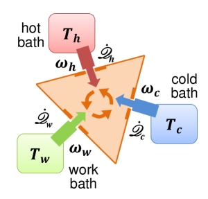
Figure 1: Quantum tricycle: A quantum system selectively coupled through frequency filters to three heat baths (with temperatures $T_{w}>T_{h}>T_{c}$), embodies the prototype of any thermal device. Here, the direction of the heat currents (depicted as arrows) correspond to a refrigerator. Reversing them realizes a heat transformer/heat engine.

II Endoreversible quantum tricycles

A generic energy conversion device may be thought of as a stationary black box in simultaneous thermal contact with three heat reservoirs at different temperatures $T_{w}>T_{h}>T_{c}$ or, alternatively, with two heat reservoirs $T_{h}>T_{c}$ and a work repository ($T_{w}\rightarrow\infty$), which, in principle, accounts for the case of a heat engine or a power-driven refrigerator (we shall elaborate more on this equivalence in an example below). This template, termed ‘tricycle’ Andresen et al. (1977), is suitable to describe averaged finite-time cycles or continuous processes, and is represented by the triple $\{\dot{\mathscr{Q}}_{w},\dot{\mathscr{Q}}_{h},\dot{\mathscr{Q}}_{c}\}$ of steady-state rates of incoming (positive) and outgoing (negative) energy flow in the system through each of the thermal contact ports. In order to comply with the first and second laws of thermodynamics, these must satisfy

$$\dot{\mathscr{Q}}_{w}+\dot{\mathscr{Q}}_{h}+\dot{\mathscr{Q}}_{c} =0$$ (2a)

$$\frac{\dot{\mathscr{Q}}_{w}}{T_{w}}+\frac{\dot{\mathscr{Q}}_{h}}{T_{h}}+\frac{\dot{\mathscr{Q}}_{c}}{T_{c}} \equiv-\dot{S}\leq 0.$$ (2b)

If the black box encloses a quantum system, thermal contact with the heat reservoir may be selectively established through filters at frequencies $\omega_{\alpha}$ with $\alpha\in\{w,h,c\}$. This is the distinctive feature of a quantum tricycle Kosloff and Levy (2014) (see Fig. 1). In absence of heat leaks or internal friction, a quantum tricycle exchanges quanta with all three baths at a single stationary rate $\mathscr{I}$, i.e. $\dot{\mathscr{Q}}_{\alpha}=-\omega_{\alpha}\mathscr{I}_{\alpha}$, with $\mathscr{I}_{h}=-\mathscr{I}_{c}=-\mathscr{I}_{w}\equiv\mathscr{I}$ (in what follows $\hbar=k_{B}=1$). Thence, the fulfilment of the first law in Eq. (2a) demands to tune the filters in resonance so that $\omega_{w}=\omega_{h}-\omega_{c}$.

Such ‘ideal’ devices have two complementary modes of operation compatible with Eq. (2b): The absorption/compression refrigerator $\{\dot{\mathscr{Q}}_{w}>0,\dot{\mathscr{Q}}_{h}<0,\dot{\mathscr{Q}}_{c}>0\}$ and the heat transformer/heat engine $\{\dot{\mathscr{Q}}_{w}<0,\dot{\mathscr{Q}}_{h}>0,\dot{\mathscr{Q}}_{c}<0\}$ Andresen et al. (1977); Gordon and Ng (2000). Let us consider for instance a compression refrigerator $(T_{w}\rightarrow\infty)$ at fixed $\omega_{h}$, for which the inequality (2b) may be rewritten as $\omega_{c}\leq\omega_{c,\,\text{rev}}\equiv\omega_{h}T_{c}/T_{h}$. As $\omega_{c}\rightarrow\omega_{c,\,\text{rev}}$, the contact ports simultaneously reach local thermal equilibrium with their respective heat reservoirs, and the COP is maximized $(\varepsilon\rightarrow\varepsilon_{C})$ Geusic et al. (1967). In general, however, the effective temperatures $T_{\alpha}^{\prime}$ defined from the stationary state of the contacts, do not coincide with the corresponding equilibrium values $T_{\alpha}$, and the COP is strictly smaller than $\varepsilon_{C}$.

The irreversibility hindering the cooling performance of ideal quantum tricycles might be thus understood as if only arising from imperfect thermal contact with the heat baths. It is in this sense that we refer to them as ‘endoreversible’. Alternatively, ideal energy conversion systems may be tagged ‘strongly coupled’ Kedem and Caplan (1965); Esposito et al. (2009), referring to the fact that their energy fluxes remain at all times proportional to each other. This is a necessary prerequisite for any device to achieve maximum efficiency, although at vanishing energy-conversion rates Kedem and Caplan (1965).

III Optimal COP for large temperatures

Next, we shall tune the frequency filters of a generic endoreversible power-driven tricycle in the refrigerator configuration, so as to maximize its cooling power in search for the optimal COP.

From Eq. (2b) it follows that the entropy production can be written as $\dot{S}=x_{h}\mathscr{I}_{h}+x_{c}\mathscr{I}_{c}$, where the fluxes are $\mathscr{I}_{h}=-\mathscr{I}_{c}\equiv\mathscr{I}$, and their conjugate thermodynamic forces are given by $x_{\alpha}\equiv\omega_{\alpha}/T_{\alpha}$. Note that refrigeration is achieved whenever $x_{c}<x_{h}$, according to Eq. (2b). Even though we shall concentrate on the dependence of the flux on the thermodynamic forces, it will generally be a function of other independent dimensionless combinations of parameters, describing the system-bath interactions and the spectrum of thermal fluctuations of the heat reservoirs.

The cold heat current writes as $|\dot{\mathscr{Q}}_{c}|=T_{c}x_{c}\mathscr{I}(x_{h},x_{c})$ and its local maximization with respect to $x_{c}$ at fixed $x_{h}$, follows from

$$x_{c,*}\frac{\partial\mathscr{I}}{\partial x_{c}}(x_{h},x_{c,*})+\mathscr{I}(x_{h},x_{c,*})=0.$$ (3)

Little more can be said without disclosing the full Hamiltonian of the tricycle, except if one restricts to a certain regime of parameters. Here, we shall take the high-temperature limit ($x_{\alpha}\rightarrow 0$), where e.g. symmetric quantum heat engines are known to operate at the Yvon-Novikov-Curzon-Ahlborn efficiency Geva and Kosloff (1996); Raam and Kosloff , and where different models of absorption refrigerators achieve their maximal performance Correa et al. (2013, 2014).

We shall thus approximate $\mathscr{I}(x_{h},x_{c})$ around $x_{\alpha}=0$, retaining only the first non-zero term in its Taylor expansion

$$\mathscr{I}(x_{h},x_{c})=\sum_{i}\left(\frac{\partial\mathscr{I}}{\partial x_{i}}\right)_{\vec{0}}x_{i}+\sum_{ij}\left(\frac{\partial^{2}\mathscr{I}}{\partial x_{i}\partial x_{j}}\right)_{\vec{0}}x_{i}x_{j}+\cdots,$$ (4)

and express the optimal ‘cold force’ as $x_{c,*}\simeq Cx_{h}$, to first order in $x_{h}$. The coefficient $C$ may be obtained by substituting the approximated current of Eq. (4) into Eq. (3), and will thus depend explicitly on the partial derivatives of the stationary heat current evaluated in $x_{\alpha}=0$. Noting that the COP of an endoreversible refrigerator writes as

$$\varepsilon=\frac{\omega_{c}}{\omega_{h}-\omega_{c}}=\left(\frac{\varepsilon_{C}+1}{\varepsilon_{C}}\frac{x_{h}}{x_{c}}-1\right)^{-1},$$ (5)

the optimal performance, normalized by $\varepsilon_{C}$, is finally

$$\frac{\varepsilon_{*}}{\varepsilon_{C}}=\frac{C}{(1-C)\,\varepsilon_{C}+1}.$$ (6)

Here, $C$ must be positive and upper-bounded by $1$, so that $0\leq\varepsilon_{*}\leq\varepsilon_{C}$. In general, it will be a function of parameters such as the dissipation rate ($\gamma$), ohmicity ($s$), high frequency cutoff ($\Omega_{c}$), dimensionality of the baths ($d$) or their equilibrium temperatures (through $\varepsilon_{C}$). Thus, and unlike Eq. (1), $\varepsilon_{*}/\varepsilon_{C}$ converges to $C(\varepsilon_{C}=0,\gamma,s,\Omega_{c},d,\cdots)$ as $\varepsilon_{C}\rightarrow 0$, rather than to a universal constant value.

The above discussion can be compared to the one done in Ref. Esposito et al. (2009) for a generic heat engine in the linear regime: There, the first order term in the expansion of the optimal force $x_{c,*}$ (in that case, around $x_{c}-x_{h}\rightarrow 0$) contributed to $\eta_{*}/\eta_{C}$ with a universal constant value of $1/2$, while the second order term added a correction, explicitly involving the first and second order partial derivatives of the heat current. In contrast, as we have just seen, the optimal cooling performance is already non-universal to the lowest order in $x_{h}$.

In order to intuitively understand this fundamental difference between engines and refrigerators, we remark that the useful effect in a heat engine is sought at the interface of the working substance with an infinite-temperature heat reservoir, implying that the corresponding contact transitions will be saturated regardless of the details of the system-bath interaction. On the contrary, in a refrigerator, the useful effect takes place in the interface with a bath at some finite temperature. Therefore, it is not so surprising that the spectral properties of the environmental fluctuations play a relevant role in establishing the optimal cooling performance.

Indeed, the situation resembles that of the maximization of the cooling power of endoreversible (‘classical’) refrigerators, for which the optimal performance is generally set by the heat conductivities, and depends critically on the specific heat transfer law assumed Yan and Chen (1990).

Finally, let us comment on the optimal COP in the complementary limit of $\varepsilon_{C}\rightarrow\infty$, that is, in the linear regime. Close to equilibrium, we may assume a linear relation between fluxes $\mathscr{I}_{\alpha}$ and forces $x_{\alpha}$, such that $\mathscr{I}_{h}=L_{11}x_{h}+L_{12}x_{c}$ and $\mathscr{I}_{c}=L_{21}x_{h}+L_{22}x_{c}$. The Onsager coefficients $L_{ij}$ satisfy $L_{11}\geq 0$, $L_{22}\geq 0$, $L_{12}=L_{21}$ and $q^{2}\equiv L_{12}^{2}/L_{11}L_{22}$. Here, the parameter $-1\leq q\leq 1$ is stands for the tightness of the coupling between input and output fluxes Kedem and Caplan (1965), where $q^{2}\rightarrow 1$ implies ‘endoreversiblity’. We can maximize again $|\dot{\mathscr{Q}}_{c}|=T_{c}x_{c}\mathscr{I}_{c}$ in $x_{c}$ for fixed $x_{h}$, obtaining $x_{c,*}=-L_{21}x_{h}/2L_{22}$. This yields an optimal COP of

$$\varepsilon_{*}=\frac{q^{2}\varepsilon_{C}}{(4-3q^{2})\varepsilon_{C}+(4-2q^{2})},$$ (7)

which converges to $\varepsilon_{*}=q^{2}/(4-3q^{2})$ as $\varepsilon_{C}\rightarrow\infty$. Hence, the ratio $\varepsilon_{*}/\varepsilon_{C}$ simply vanishes close to equilibrium, regardless of the magnitude of $x_{\alpha}$ and the details system-bath coupling.

IV Example: Unstructured bosonic baths

In order to get a closed expression for $C(\varepsilon_{C},\gamma,s,\Omega_{c},d,\cdots)$, specific instances have to be considered. Here we focus on a simple and paradigmatic endoreversible device, such as a three-level maser Scovil and Schulz-DuBois (1959) subject to a weak periodic driving, in contact with unstructured bosonic baths (i.e. characterized by a flat spectral density) in $d_{\alpha}$ dimensions. Its Hamiltonian writes as

$$H=\omega_{c}\left|2\right\rangle\left\langle 2\right|+\omega_{h}\left|3\right\rangle\left\langle 3\right|+\lambda\left(e^{i\omega_{w}t}\left|2\right\rangle\left\langle 3\right|+e^{-i\omega_{w}t}\left|3\right\rangle\left\langle 2\right|\right),$$ (8)

where $\lambda$ is the intensity of the driving at the power input transition $\left|2\right\rangle\leftrightarrow\left|3\right\rangle$. The remaining ones ($\left|1\right\rangle\leftrightarrow\left|3\right\rangle$ and $\left|1\right\rangle\leftrightarrow\left|2\right\rangle$), are linearly connected with the ‘hot’ and ‘cold’ heat reservoirs, through terms of the form $\sigma_{\alpha}\otimes\mathscr{B}_{\alpha}$, where

$$\mathscr{B}_{\alpha} \equiv\sum\nolimits_{\mu}g_{\alpha\mu}\left(b_{\alpha\mu}+b_{\alpha\mu}^{\dagger}\right)$$ (9a)

$$\sigma_{h} \equiv\left|1\right\rangle\left\langle 3\right|+\left|3\right\rangle\left\langle 1\right|$$ (9b)

$$\sigma_{c} \equiv\left|1\right\rangle\left\langle 2\right|+\left|2\right\rangle\left\langle 1\right|.$$ (9c)

The constants $g_{\alpha\mu}\propto(\gamma_{\alpha}\omega_{\mu})^{1/2}$ indicate the intensity of the coupling between the mode $\omega_{\mu}$ of bath $\alpha$ and the corresponding contact transition of the working substance, and $\gamma_{\alpha}$ stands for the dissipation strength Correa et al. (2013).

We shall assume very weak dissipation (i.e. $\gamma_{\alpha}\ll T_{\alpha}$) and parameters well into the quantum optical regime, so as to consistently derive a quantum master equation like $\dot{\varrho}=\sum_{\alpha}\sum_{\omega}\sum_{q\in\mathbb{Z}}\,\mathscr{L}^{\alpha}_{\omega,q}\,\varrho$, with dissipators $\mathscr{L}^{\alpha}_{\omega,q}$ of the Lindblad-Gorini-Kossakowski-Sudarshan type Lindblad (1976); Gorini et al. (1976). Their explicit form is given in Appendix A.

The non-equilibrium limit cycle state $\varrho_{\infty}$ may be found from $\sum_{\alpha}\sum_{\omega}\sum_{q\in\mathbb{Z}}\,\mathscr{L}^{\alpha}_{\omega,q}\,\varrho_{\infty}=0$, while the corresponding (time-averaged) heat currents are Robert Alicki (2012)

$$\dot{\mathscr{Q}}_{\alpha}=-T_{\alpha}\sum_{\omega}\sum_{q\in\mathbb{Z}}\text{tr}\{\mathscr{L}^{\alpha}_{\omega,q}\,\varrho_{\infty}\ln{\tilde{\varrho}^{\alpha}_{\omega,q}}\}.$$ (10)

The states $\tilde{\varrho}^{\alpha}_{\omega,q}$ are the unique local stationary states of each dissipator, i.e. $\mathscr{L}^{\alpha}_{\omega,q}\,\tilde{\varrho}^{\alpha}_{\omega,q}=0$.

In general, a power-driven three-level maser does not realize a tricycle as it features closed performance characteristics, which is a clear indicator of irreversibility Kosloff and Levy (2014). We shall take, however, the limit of weak driving, i.e. $\lambda\rightarrow 0$, in which the time averaged limit flux $\mathscr{I}$ reads

$$\mathscr{I}\simeq\frac{\Gamma_{\omega_{h}}\Gamma_{-\omega_{c}}-\Gamma_{-\omega_{h}}\Gamma_{\omega_{c}}}{\Gamma_{\omega_{h}}+\Gamma_{\omega_{c}}+2\big{(}\Gamma_{-\omega_{h}}+\Gamma_{-\omega_{c}}\big{)}}.$$ (11)

The excitation and relaxation rates $\Gamma_{\pm\omega_{\alpha}}$ are given by $\Gamma_{\omega_{\alpha}}\equiv\gamma_{\alpha}\omega^{d_{\alpha}}[N(\omega_{\alpha})+1]$ and $\Gamma_{-\omega_{\alpha}}=e^{-\omega_{\alpha}/T_{\alpha}}\Gamma_{\omega_{\alpha}}$, with $N(\omega_{\alpha})\equiv(e^{\omega_{\alpha}/T_{\alpha}}-1)^{-1}$. Here, $d_{\alpha}$ stands for the physical dimensionality of bath $\alpha$ Breuer and Petruccione (2002).

Taking now the high-temperature limit would result in $\Gamma_{\omega_{\alpha}}\simeq\gamma_{\alpha}T_{\alpha}\omega_{\alpha}^{d_{\alpha}-1}$ and $\Gamma_{-\omega_{\alpha}}\simeq\gamma_{\alpha}T_{\alpha}\omega_{\alpha}^{d_{\alpha}-1}(1-x_{\alpha})$, so that

$$\mathscr{I}\simeq\frac{\gamma_{h}\gamma_{c}}{3}T_{c}\,\omega_{c}^{d_{c}-1}\frac{\omega_{h}/T_{h}-\omega_{c}/T_{c}}{\gamma_{h}+\omega_{c}^{d_{c}-1}\omega_{h}^{1-d_{h}}\gamma_{c}T_{c}/T_{h}}.$$ (12)

We shall discard the second term in the denominator of Eq. (12) by assuming that the coupling to the entropy sink is much stronger than the interaction with the cold bath (i.e. $\gamma_{c}\ll\gamma_{h}$). Setting up a comparatively efficient heat rejection mechanism is indeed very important for the maximization of the stationary flux in a refrigerator, which justifies this assumption as a first step towards optimality. Nonetheless, noting that $T_{c}/T_{h}=\varepsilon_{C}/(\varepsilon_{C}+1)$, we see that this would be justified anyway, as long as $\varepsilon_{C}\rightarrow 0$. The stationary flux may be thus written as

$$\mathscr{I}\simeq\mathscr{I}_{0}(x_{c}^{d_{c}-1}x_{h}-x_{c}^{d_{c}}),$$ (13)

with $\mathscr{I}_{0}=\gamma_{c}T_{c}^{d_{c}}/3$. From here, it follows that $C\equiv d_{c}/(d_{c}+1)$, i.e. $x_{c,*}=d_{c}/(d_{c}+1)\,\omega_{h}$, which once substituted in Eq. (6) yields the following simple performance benchmark,

$$\frac{\varepsilon_{*}}{\varepsilon_{C}}=\frac{d_{c}}{d_{c}+1+\varepsilon_{C}}.$$ (14)

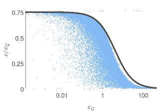
Figure 2: (Blue dots) Optimal normalized COP versus $\varepsilon_{C}$ for about $2\times 10^{5}$ $n$–stage endoreversible absorption refrigerators Correa (2014) with $n\in\{1,\cdots,10\}$, and coupled to unstructured three-dimensional bosonic baths. All three temperatures $T_{\alpha}$, dissipation rates $\gamma_{\alpha}$ and hot frequencies $\omega_{h}$ were picked at random, and the COP was optimized in $\omega_{c}$ so as to maximize the cooling power $\dot{\mathscr{Q}}_{c}$ in each case. Eq. (14) is plotted in solid gray.

In Fig. 2, the optimal normalized COP of a large number of single- and multi-stage endoreversible absorption refrigerators Correa (2014) is compared with Eq. (14), considering unstructured bosonic baths with dimensionality $d_{\alpha}=3$. We observe a remarkable agreement, especially at low $\varepsilon_{C}$. Notice, however, that Eq. (14) was obtained for a specific model of compression refrigerator and under the assumption of asymmetric dissipation: There is, in principle, no reason, why it should remain tight nor an upper bound to the performance of other endoreversible models. Therefore, it should be thought-of just as a reasonable approximation to their generic behaviour. On a second thought, however, the excellent agreement observed may not be so surprising, provided that the optimal performance is set by the dissipative scheme alone. Solving for the limit cycle of a (weakly-driven) compression tree-level maser in different types of environment would be thus enough to come up with generally valid benchmarks for any endoreversible refrigerator in each case. This is one of the take-home messages of the present paper.

The optimal performance of single and multi-stage quantum absorption refrigerators is indeed known to be limited by $\varepsilon_{*}/\varepsilon_{C}\leq d/(d+1)$ when attached to unstructured baths in $d$ dimensions, with a saturation occurring precisely in the limit of large temperatures Correa et al. (2014); Correa (2014). Eq. (14) can be thus regarded for these models as a stronger bound which sharpens the one given in Ref. Correa (2014) for any finite $\varepsilon_{C}$. Remarkably, also another model of non-ideal refrigerator, with the same dissipative scheme, has been shown to have an optimal performance below $\varepsilon_{*}/\varepsilon_{C}=d/(d+1)$ Correa et al. (2013). Note, however that Eq. (14) should not be expected to hold quantitatively (and not even as a qualitative indicator of optimality) when moving away from endoreversibility.

V Conclusions

To summarize and conclude, we have shown from first principles how the COP at maximum cooling power of endoreversible quantum tricycles is not universal in the high-temperature limit, but fundamentally constrained by the details of their interaction with the external heat reservoirs. For quantum refrigerators coupled to unstructured bosonic baths, we obtained a compact expression for their optimal performance, only dependent on the Carnot COP and the dimensionality of the baths.

Our results highlight the importance of reservoir engineering Poyatos et al. (1996) in the design of quantum thermal devices: While squeezed-thermal and other types of engineered non-equilibrium environments are known to be capable of enhancing both the performance and power of heat engines and quantum refrigerators Huang et al. (2012); Abah and Lutz (2014); Roßnagel et al. (2014); Correa et al. (2014), the exploration of more exotic and highly tunable reservoirs, such as cold atomic gases McEndoo et al. (2013), might bring about new possibilities for the physical realization of super-efficient thermodynamic cycles, especially interesting for practical applications to quantum technologies.

Appendix A Master equation for a periodically-driven three-level maser

In what follows, we shall derive a quantum master equation for a three-level maser weakly coupled to two unstructured bosonic reservoirs in $d$ dimensions, and driven by a periodic perturbation. As already stated in the main text, the full Hamiltonian of system and baths (excluding their mutual interactions) is given by

$$H_{0}(t)=H(t)+H_{B}=\omega_{c}\left|2\right\rangle\left\langle 2\right|+\omega_{h}\left|3\right\rangle\left\langle 3\right|+\\ \lambda\left(e^{i\omega_{w}t}\left|2\right\rangle\left\langle 3\right|+e^{-i\omega_{w}t}\left|3\right\rangle\left\langle 2\right|\right)+\sum_{\alpha=\{h,c\}}\sum_{\lambda}\omega_{\lambda}b_{\alpha\lambda}^{\dagger}b_{\alpha\lambda},$$ (15)

while the system-bath coupling writes as

$$H_{I}=\sum_{\alpha=\{h,c\}}\sigma_{\alpha}\otimes\left(\sum_{\lambda}g_{\alpha\lambda}(b_{\alpha\lambda}+b^{\dagger}_{\alpha\lambda})\right).$$ (16)

Recall that the ‘thermal contact’ operators $\sigma_{\alpha}$ were just $\sigma_{h}\equiv\left|1\right\rangle\left\langle 3\right|+\left|3\right\rangle\left\langle 1\right|$ and $\sigma_{c}\equiv\left|1\right\rangle\left\langle 2\right|+\left|2\right\rangle\left\langle 1\right|$. The standard recipe to derive a Lindbland-Gorini-Kossakovsky-Sudarshan quantum master equation Breuer and Petruccione (2002) demands to express the two $\sigma_{\alpha}$ in the interaction picture with respect to $H_{0}(t)$, and then, to suitably decompose them.

In the present case, the unitary evolution operator associated with $H_{0}(t)$ is formally given by the time-ordered exponential $U_{0}(t)=\mathscr{T}\exp\left\{-i\int_{0}^{t}ds~{}H_{0}(s)\right\}$, and may be written as $U_{0}(t)=U_{1}(t)U_{2}(t)\otimes e^{-iH_{B}t}$, where

$$U_{1}(t) \equiv\exp{\left\{-it\left(\omega_{c}\left|2\right\rangle\left\langle 2\right|+\omega_{h}\left|3\right\rangle\left\langle 3\right|\right)\right\}}$$ (17a)

$$U_{2}(t) \equiv\exp{\left\{-it\lambda\left(\left|2\right\rangle\left\langle 3\right|+\omega_{h}\left|3\right\rangle\left\langle 2\right|\right)\right\}}.$$ (17b)

This may be easily checked by noticing that $\frac{d}{dt}\left\{U_{1}(t)U_{2}(t)\right\}=-iH(t)U_{1}(t)U_{2}(t)$.

A time-independent (or time-averaged) Hamiltonian $\bar{H}$ can be defined, that generates the same unitary dynamics as $U(t)$ [i.e. $e^{-i\bar{H}t}\equiv U_{1}(t)U_{2}(t)$]. For our three-level maser, this would be

$$\bar{H}=\omega_{c}\left(\left|2\right\rangle\left\langle 2\right|+\left|3\right\rangle\left\langle 3\right|\right)+\lambda\left(\left|2\right\rangle\left\langle 3\right|+\left|3\right\rangle\left\langle 2\right|\right),$$ (18)

with eigenvalues $\epsilon=\{0,\omega_{c}-\lambda,\omega_{c}+\lambda\}$. Its corresponding set of positive Bohr quasi-frequencies ($\epsilon_{j}-\epsilon_{i}>0$) is thus $\bar{\omega}=\{0,2\lambda,\omega_{c}\pm\lambda\}$, where we have assumed without loss of generality that $\omega_{c}>\lambda$.

In general, we would have to resort now to Floquet theory Robert Alicki (2012); Szczygielski et al. (2013) in order to decompose the interaction picture thermal contact operators as

$$U(t)^{\dagger}\sigma_{\alpha}U(t)=\sum_{\bar{\omega}}\sum_{q\in\mathbb{Z}}A_{\bar{\omega},q}^{\alpha}e^{-i(\bar{\omega}+q\omega_{w})t}.$$ (19)

Fortunately for us, this may be done by mere inspection of the left-hand side of Eq. (19), resulting in

$$A^{h}_{\omega_{c}+\lambda,1} =\frac{1}{2}\left(\left|1\right\rangle\left\langle 3\right|+\left|1\right\rangle\left\langle 2\right|\right)$$ (20a)

$$A^{h}_{\omega_{c}-\lambda,1} =\frac{1}{2}\left(\left|1\right\rangle\left\langle 3\right|-\left|1\right\rangle\left\langle 2\right|\right)$$ (20b)

$$A^{c}_{\omega_{c}+\lambda,0} =\frac{1}{2}\left(\left|1\right\rangle\left\langle 2\right|+\left|1\right\rangle\left\langle 3\right|\right)$$ (20c)

$$A^{c}_{\omega_{c}-\lambda,0} =\frac{1}{2}\left(\left|1\right\rangle\left\langle 2\right|-\left|1\right\rangle\left\langle 3\right|\right)$$ (20d)

$$A^{\alpha}_{-\bar{\omega},-q}={A^{\alpha}_{\bar{\omega},q}}^{\dagger}.$$ (20e)

There are, therefore, two open decay channels for each thermal contact, corresponding to frequencies $\omega_{\alpha}\pm\lambda$ ($\omega_{w}=\omega_{h}-\omega_{c}$).

Provided with the decomposition of Eq. (20e), we can now successively apply the Born, Markov and rotating-wave (or secular) approximations on the effective equation of motion of the reduced density operator of the system in the interaction picture $\varrho(t)$ Robert Alicki (2012); Breuer and Petruccione (2002). We thus arrive to a quantum master equation in the standard form:

$$\frac{d\varrho}{dt}=\sum_{\alpha}\sum_{\bar{\omega}}\sum_{q\in\mathbb{Z}}\mathscr{L}_{\bar{\omega},q}^{\alpha}[\varrho]\\ \equiv\sum_{\alpha}\sum_{\bar{\omega}}\sum_{q\in\mathbb{Z}}\left[\Gamma_{\bar{\omega},q}^{\alpha}\left(A_{\bar{\omega},q}^{\alpha}\varrho{A_{\bar{\omega},q}^{\alpha}}^{\dagger}-\frac{1}{2}\{{A_{\bar{\omega},q}^{\alpha}}^{\dagger}A_{\bar{\omega},q}^{\alpha},\varrho\}_{+}\right)+\right.\\ \left.\Gamma_{-\bar{\omega},-q}^{\alpha}\left({A_{\bar{\omega},q}^{\alpha}}^{\dagger}\varrho A_{\bar{\omega},q}^{\alpha}-\frac{1}{2}\{A_{\bar{\omega},q}^{\alpha}{A_{\bar{\omega},q}^{\alpha}}^{\dagger},\varrho\}_{+}\right)\right].$$ (21)

The assumption of factorized initial conditions between system and environmental degrees of freedom is implicit in the above, as is thermal equilibrium for the hot and cold heat reservoirs. Also note that the Lamb-shift term has been neglected in Eq. (21).

The relaxation rates $\Gamma_{\omega}^{\alpha}=2\text{Re}\left\{\int_{0}^{\infty}ds~{}e^{i\omega s}\left\langle B_{\alpha}(t)B_{\alpha}(t-s)\right\rangle\right\}$ are determined by the power spectrum of the environmental fluctuations, and satisfy the Kubo-Martin-Schwinger condition Kubo (1957); Martin and Schwinger (1959) $\Gamma_{-\omega}^{\alpha}=e^{-\omega/T_{\alpha}}\Gamma_{\omega}^{\alpha}$. Here, $\left\langle\cdots\right\rangle$ stands for equilibrium averaging. As already advanced in the main text, for our choice of the system-baths coupling scheme, i.e. bosonic baths with constant spectral density $J_{\alpha}(\omega)\sim\gamma_{\alpha}$, the relaxation rates are explicitly given by $\Gamma_{\omega}^{\alpha}=\gamma_{\alpha}\omega^{d_{\alpha}}[N_{\alpha}(\omega)+1]$, with $N_{\alpha}(\omega)\equiv(e^{\omega/T_{\alpha}}-1)^{-1}$. Physically, this is compatible with weak coupling to the quantized electromagnetic field in thermal equilibrium, inside a $d_{\alpha}$–dimensional box Breuer and Petruccione (2002).

Equipped with Eqs. (20e) and (21), we are now in the position of finding the limit cycle state $\varrho_{\infty}$, which is defined as

$$\sum_{\alpha}\sum_{\bar{\omega}}\sum_{q\in\mathbb{Z}}\mathscr{L}_{\bar{\omega},q}^{\alpha}[\varrho_{\infty}]=0.$$ (22)

The dissipators $\mathscr{L}_{\bar{\omega},q}^{\alpha}$ have local steady states (i.e. $\mathscr{L}^{\alpha}_{\bar{\omega},q}[\tilde{\varrho}_{\bar{\omega},q}^{\alpha}]=0$) of the form $\tilde{\varrho}^{\alpha}_{\bar{\omega},q}=Z^{-1}\exp\left\{-\frac{\bar{\omega}+q\omega_{w}}{\bar{\omega}}\bar{H}\right\}$ Robert Alicki (2012). Given their standard Lindblad form, each $\mathscr{L}^{\alpha}_{\bar{\omega},q}$ individually generates a fully contractive reduced dynamics towards $\tilde{\varrho}^{\alpha}_{\bar{\omega},q}$, which is reflected in the monotonic decrease of the distance, as measured by the relative entropy, from any locally evolved state $\frac{d}{dt}\varrho(t)=\mathscr{L}^{\alpha}_{\bar{\omega},q}[\varrho(t)]$ to $\tilde{\varrho}^{\alpha}_{\bar{\omega},q}$ [i.e. $\frac{d}{dt}S(\varrho(t)||\tilde{\varrho}^{\alpha}_{\omega,q})\leq 0$] Spohn (1978); Breuer and Petruccione (2002). Such contractivity property applied to the actual steady state of the full Eq. (21) eventually leads to the following inequality Robert Alicki (2012)

$$\sum_{\alpha}\frac{1}{T_{\alpha}}\left(-T_{\alpha}\sum_{\bar{\omega}}\sum_{q\in\mathbb{Z}}\text{Tr}~{}\mathscr{L}^{\alpha}_{\bar{\omega},q}[\varrho_{\infty}]\log\tilde{\varrho}_{\bar{\omega},q}^{\alpha}\right)\leq 0,$$ (23)

or equivalently

$$\sum_{\alpha}\frac{1}{T_{\alpha}}\left(\sum_{\bar{\omega}}\sum_{q\in\mathbb{Z}}\frac{\bar{\omega}+q\omega_{w}}{\bar{\omega}}~{}\text{Tr}~{}\bar{H}\mathscr{L}^{\alpha}_{\bar{\omega},q}[\varrho_{\infty}]\right)\leq 0.$$ (24)

This can be understood as a statement of the second law of thermodynamics upon defining the limit cycle heat currents as $\dot{\mathscr{Q}}_{\alpha}\equiv\sum_{\bar{\omega}}\sum_{q\in\mathbb{Z}}\frac{\bar{\omega}+q\omega_{w}}{\bar{\omega}}~{}\text{Tr}\{\bar{H}\mathscr{L}^{\alpha}_{\bar{\omega},q}[\varrho_{\infty}]\}$ Robert Alicki (2012).

As it is probably useful for the interested reader, we now detail the specific form of the hot and cold dissipators. These are given by

$${\cal L}_{\omega_{\alpha}+\lambda}^{\alpha}[\varrho] = \frac{\Gamma_{\omega_{\alpha}+\lambda}}{4}{\cal D}_{++}[\varrho]\,+\,\frac{\Gamma_{-\omega_{\alpha}-\lambda}}{4}{\cal D}_{--}[\varrho]\,,$$

$${\cal L}_{\omega_{\alpha}-\lambda}^{\alpha}[\varrho] = \frac{\Gamma_{\omega_{\alpha}-\lambda}}{4}{\cal D}_{+-}[\varrho]\,+\,\frac{\Gamma_{-\omega_{\alpha}+\lambda}}{4}{\cal D}_{-+}[\varrho]\,,$$ (25)

To simplify the notation, we have introduced the superoperators ${\cal D}$, which act on $\varrho$ as

$${\cal D}_{++}[\varrho] = (|1\rangle\langle 2|+|1\rangle\langle 3|)\varrho(|2\rangle\langle 1|+|3\rangle\langle 1|)$$

$$- \frac{1}{2}(|2\rangle\langle 2|+|2\rangle\langle 3|+|3\rangle\langle 2|+|3\rangle\langle 3|)\varrho$$

$$- \frac{1}{2}\varrho(|2\rangle\langle 2|+|2\rangle\langle 3|+|3\rangle\langle 2|+|3\rangle\langle 3|)\,,$$

$${\cal D}_{--}[\varrho] = (|2\rangle\langle 1|+|3\rangle\langle 1|)\varrho(|1\rangle\langle 2|+|1\rangle\langle 3|)$$

$$- |1\rangle\langle 1|\varrho-\varrho|1\rangle\langle 1|\,,$$

$${\cal D}_{+-}[\varrho] = (|1\rangle\langle 2|-|1\rangle\langle 3|)\varrho(|2\rangle\langle 1|-|3\rangle\langle 1|)$$

$$- \frac{1}{2}(|2\rangle\langle 2|-|2\rangle\langle 3|-|3\rangle\langle 2|+|3\rangle\langle 3|)\varrho$$

$$- \frac{1}{2}\varrho(|2\rangle\langle 2|-|2\rangle\langle 3|-|3\rangle\langle 2|+|3\rangle\langle 3|)\,,$$

$${\cal D}_{-+}[\varrho] = (|2\rangle\langle 1|-|3\rangle\langle 1|)\varrho(|1\rangle\langle 2|-|1\rangle\langle 3|)$$ (26)

$$- |1\rangle\langle 1|\varrho-\varrho|1\rangle\langle 1|\,.$$

The populations of the limit cycle state $\varrho_{\infty}$ (expressed in vector form as $\mathbf{n}=\{n_{1},n_{2},n_{3}\}$) may be found by combining the relation ${\mathbb{M}}^{D3L}\cdot{\bf n}=\mathbf{0}$ with the normalisation condition $\sum_{i}\,n_{i}=1$. The coefficient matrix ${\mathbb{M}}^{D3L}$ is given by

$${\mathbb{M}}^{D3L}=\left(\begin{array}[]{ccc}-2G^{+}_{-\omega}+2\frac{G^{-}_{\omega}G^{-}_{-\omega}}{G^{+}_{\omega}}&G^{+}_{\omega}-\frac{G^{-}_{\omega}G^{-}_{\omega}}{G^{+}_{\omega}}&G^{+}_{\omega}-\frac{G^{-}_{\omega}G^{-}_{\omega}}{G^{+}_{\omega}}\\ G^{+}_{-\omega}-\frac{G^{-}_{\omega}G^{-}_{-\omega}}{G^{+}_{\omega}}&-G^{+}_{\omega}+\frac{G^{-}_{\omega}G^{-}_{\omega}}{2G^{+}_{\omega}}&\frac{G^{-}_{\omega}G^{-}_{\omega}}{2G^{+}_{\omega}}\\ G^{+}_{-\omega}-\frac{G^{-}_{\omega}G^{-}_{-\omega}}{G^{+}_{\omega}}&\frac{G^{-}_{\omega}G^{-}_{\omega}}{2G^{+}_{\omega}}&-G^{+}_{\omega}+\frac{G^{-}_{\omega}G^{-}_{\omega}}{2G^{+}_{\omega}}\end{array}\right)\,,$$ (27)

where the constants $G^{\pm}_{\omega}$ are defined as

$$\begin{array}[]{cc}G^{+}_{\omega}\,\equiv\,\frac{\Gamma^{S}_{\omega+\lambda}+\Gamma^{S}_{\omega-\lambda}}{4}\,,&G^{+}_{-\omega}\,\equiv\,\frac{\Gamma^{S}_{-\omega-\lambda}+\Gamma^{S}_{-\omega+\lambda}}{4}\,,\\ G^{-}_{\omega}\,\equiv\,\frac{\Gamma^{S}_{\omega+\lambda}-\Gamma^{S}_{\omega-\lambda}}{4}\,,&G^{-}_{-\omega}\,\equiv\,\frac{\Gamma^{S}_{-\omega-\lambda}-\Gamma^{S}_{-\omega+\lambda}}{4}\,,\end{array},$$ (28)

and $\Gamma^{S}_{\pm\omega\pm\lambda}\,\equiv\,\Gamma^{\alpha}_{\pm\omega_{h}\pm\lambda}\,+\,\Gamma^{\alpha}_{\pm\omega_{c}\pm\lambda}$.

Finally, we also give the explicit form of the cycle-averaged stationary heat flows. In particular, $\dot{\mathscr{Q}}_{h}$ is given by

$$\dot{\cal Q}_{h}\,=\,\dot{\cal Q}_{\omega_{h}+\lambda}\,+\,\dot{\cal Q}_{\omega_{h}-\lambda}\,,$$

$$\dot{\cal Q}_{\omega_{h}+\lambda}\,=\,\frac{\omega_{h}+\lambda}{\omega_{c}+\lambda}\,{\rm Tr}\{\bar{H}{\cal L}_{\omega_{h}+\lambda}[\tilde{\rho}]\}=\,$$

$$(\omega_{h}+\lambda)\left[\frac{\Gamma_{-\omega_{h}-\lambda}}{2}n_{1}\,-\,\frac{\Gamma_{\omega_{h}+\lambda}}{4}(n_{2}+n_{3}+n_{c})\right]\,,$$

$$\dot{\cal Q}_{\omega_{h}-\lambda}\,=\,\frac{\omega_{h}-\lambda}{\omega_{c}-\lambda}\,{\rm Tr}\{\bar{H}{\cal L}_{\omega_{h}-\lambda}[\tilde{\rho}]\}\,=\,$$

$$(\omega_{h}-\lambda)\left[\frac{\Gamma_{-\omega_{h}+\lambda}}{2}n_{1}\,-\,\frac{\Gamma_{\omega_{h}-\lambda}}{4}(n_{2}+n_{3}-n_{c})\right]\,,$$

and $\dot{\mathscr{Q}}_{c}$ writes as

$$\dot{\cal Q}_{c}\,=\,\dot{\cal Q}_{\omega_{c}+\lambda}\,+\,\dot{\cal Q}_{\omega_{c}-\lambda}\,,$$

$$\dot{\cal Q}_{\omega_{c}+\lambda}\,=\,{\rm Tr}\{\bar{H}{\cal L}_{\omega_{c}+\lambda}[\tilde{\rho}]\}$$

$$=(\omega_{c}+\lambda)\left[\frac{\Gamma_{-\omega_{c}-\lambda}}{2}n_{1}\,-\,\frac{\Gamma_{\omega_{c}+\lambda}}{4}(n_{2}+n_{3}+n_{c})\right]\,,$$

$$\dot{\cal Q}_{\omega_{c}-\lambda}\,=\,{\rm Tr}\{\bar{H}{\cal L}_{\omega_{c}-\lambda}[\tilde{\rho}]\}$$

$$=(\omega_{c}-\lambda)\left[\frac{\Gamma_{-\omega_{c}+\lambda}}{2}n_{1}\,-\,\frac{\Gamma_{\omega_{c}-\lambda}}{4}(n_{2}+n_{3}-n_{c})\right]\,.$$

In these expressions, the constant $n_{c}$ is defined as

$$n_{c}\,\equiv\,(n_{23}+n_{32})\,=\,2\frac{G^{-}_{-\omega}}{G^{+}_{\omega}}\,n_{1}\,-\,\frac{G^{-}_{\omega}}{G^{+}_{\omega}}(n_{2}+n_{3})\,,$$ (29)

where $n_{ij}=\langle i|\varrho_{\infty}|j\rangle$ stands for steady-state coherences.

Getting the steady-state populations from Eq. (27) and using the xpressions for the heat currents above, allows to check the validity of Eq. (11) in the limit of $\lambda\rightarrow 0$.

References

• Andresen (2011) B. Andresen, Angewandte Chemie International Edition 50, 2690 (2011).
• Hoffmann et al. (1997) K. H. Hoffmann, J. M. Burzler, and S. Schubert, J. Non-Equilib. Thermodyn 22, 311 (1997).
• Novikov (1957) I. Novikov, Atomic Energy 3, 1269 (1957).
• Carnot (1890) S. Carnot, Reflections on the Motive Power of Heat and on Machines Fitted to Develop That Power (J. Wiley & Sons (New York), 1890).
• Yvon (1955) J. Yvon, in Proceedings of the International Conference on Peaceful Uses of Atomic Energy (United Nations, Geneva) (1955), p. 387.
• Curzon and Ahlborn (1975) F. Curzon and B. Ahlborn, Am. J. Phys. 43, 22 (1975).
• (7) A. Vaudrey, F. Lanzetta, and M. Feidt, e-print arXiv:1406.5853.
• Van den Broeck (2005) C. Van den Broeck, Phys. Rev. Lett. 95, 190602 (2005).
• Esposito et al. (2009) M. Esposito, K. Lindenberg, and C. Van den Broeck, Phys. Rev. Lett. 102, 130602 (2009).
• Esposito et al. (2010a) M. Esposito, R. Kawai, K. Lindenberg, and C. Van den Broeck, Phys. Rev. Lett. 105, 150603 (2010a).
• Esposito et al. (2010b) M. Esposito, R. Kawai, K. Lindenberg, and C. Van den Broeck, Phys. Rev. E 81, 041106 (2010b).
• Geva and Kosloff (1992) E. Geva and R. Kosloff, The Journal of chemical physics 96, 3054 (1992).
• Yan and Chen (1990) Z. Yan and J. Chen, Journal of Physics D: Applied Physics 23, 136 (1990).
• de Tomás et al. (2012) C. de Tomás, A. C. Hernández, and J. M. M. Roco, Phys. Rev. E 85, 010104 (2012).
• Velasco et al. (1997) S. Velasco, J. M. M. Roco, A. Medina, and A. C. Hernández, Phys. Rev. Lett. 78, 3241 (1997).
• Jiménez de Cisneros et al. (2006) B. Jiménez de Cisneros, L. A. Arias-Hernández, and A. C. Hernández, Phys. Rev. E 73, 057103 (2006).
• Chen (1994) J. Chen, Journal of Physics A: Mathematical and General 27, 6395 (1994).
• Apertet et al. (2013) Y. Apertet, H. Ouerdane, A. Michot, C. Goupil, and P. Lecoeur, EPL (Europhysics Letters) 103, 40001 (2013).
• Kosloff and Levy (2014) R. Kosloff and A. Levy, Anual Rev. Phys. Chem. 65, 365 (2014).
• Scovil and Schulz-DuBois (1959) H. E. D. Scovil and E. O. Schulz-DuBois, Phys. Rev. Lett. 2, 262 (1959).
• Palao et al. (2001) J. P. Palao, R. Kosloff, and J. M. Gordon, Phys. Rev. E 64, 056130 (2001).
• Andresen et al. (1977) B. Andresen, P. Salamon, and R. S. Berry, The Journal of Chemical Physics 66, 1571 (1977).
• Gordon and Ng (2000) J. M. Gordon and K. C. Ng, Cool thermodynamics (Cambridge international science publishing Cambridge, 2000).
• Geusic et al. (1967) J. E. Geusic, E. O. Schulz-DuBios, and H. E. D. Scovil, Phys. Rev. 156, 343 (1967).
• Kedem and Caplan (1965) O. Kedem and S. R. Caplan, Trans. Faraday Soc. 61, 1897 (1965).
• Geva and Kosloff (1996) E. Geva and R. Kosloff, J. Chem. Phys. 104, 7681 (1996).
• (27) U. Raam and R. Kosloff, e-print arXiv:1406.6788.
• Correa et al. (2013) L. A. Correa, J. P. Palao, G. Adesso, and D. Alonso, Phys. Rev. E 87, 042131 (2013).
• Correa et al. (2014) L. A. Correa, J. P. Palao, D. Alonso, and G. Adesso, Sci. Rep. 4 (2014).
• Lindblad (1976) G. Lindblad, Comm. Math. Phys. 48, 119 (1976).
• Gorini et al. (1976) V. Gorini, A. Kossakowski, and E. Sudarshan, J. Math. Phys. 17, 821 (1976).
• Robert Alicki (2012) G. K. Robert Alicki, David Gelbwaser-Klimovsky (2012).
• Breuer and Petruccione (2002) H. Breuer and F. Petruccione, The Theory of Open Quantum Systems (Oxford University Press, USA, 2002).
• Correa (2014) L. A. Correa, Phys. Rev. E 89, 042128 (2014).
• Poyatos et al. (1996) J. F. Poyatos, J. I. Cirac, and P. Zoller, Phys. Rev. Lett. 77, 4728 (1996).
• Huang et al. (2012) X. L. Huang, T. Wang, and X. X. Yi, Phys. Rev. E 86, 051105 (2012).
• Abah and Lutz (2014) O. Abah and E. Lutz, EPL (Europhysics Letters) 106, 20001 (2014).
• Roßnagel et al. (2014) J. Roßnagel, O. Abah, F. Schmidt-Kaler, K. Singer, and E. Lutz, Phys. Rev. Lett. 112, 030602 (2014).
• McEndoo et al. (2013) S. McEndoo, P. Haikka, G. D. Chiara, G. M. Palma, and S. Maniscalco, EPL (Europhysics Letters) 101, 60005 (2013).
• Szczygielski et al. (2013) K. Szczygielski, D. Gelbwaser-Klimovsky, and R. Alicki, Phys. Rev. E 87, 012120 (2013).
• Kubo (1957) R. Kubo, Journal of the Physical Society of Japan 12, 570 (1957).
• Martin and Schwinger (1959) P. C. Martin and J. Schwinger, Phys. Rev. 115, 1342 (1959).
• Spohn (1978) H. Spohn, Journal of Mathematical Physics 19, 1227 (1978).