Evidence against a mean-field description of short-range spin glasses revealed through thermal boundary conditions

Abstract

A theoretical description of the low-temperature phase of short-range spin glasses has remained elusive for decades. In particular, it is unclear if theories that assert a single pair of pure states, or theories that are based on infinitely many pure states—such as replica symmetry breaking—best describe realistic short-range systems. To resolve this controversy, the three-dimensional Edwards-Anderson Ising spin glass in thermal boundary conditions is studied numerically using population annealing Monte Carlo. In thermal boundary conditions all eight combinations of periodic vs antiperiodic boundary conditions in the three spatial directions appear in the ensemble with their respective Boltzmann weights, thus minimizing finite-size corrections due to domain walls. From the relative weighting of the eight boundary conditions for each disorder instance a sample stiffness is defined, and its typical value is shown to grow with system size according to a stiffness exponent. An extrapolation to the large-system-size limit is in agreement with a description that supports the droplet picture and other theories that assert a single pair of pure states. The results are, however, incompatible with the mean-field replica symmetry breaking picture, thus highlighting the need to go beyond mean-field descriptions to accurately describe short-range spin-glass systems.

I Introduction

A plethora of problems across disciplines and, in particular, a wide variety of optimization problems map onto spin-glass-like Hamiltonians Binder and Young (1986); Mézard et al. (1987); Young (1998); Hartmann and Rieger (2004); Stein and Newman (2013); Lucas (2014). As such, despite the fact that only a selected class of disordered magnets, such as ${\rm LiHoF_{4}}$ or ${\rm Au_{x}Fe_{1-x}}$ show this intriguing state of matter, spin glasses have been of great importance across multiple fields including condensed matter physics, evolutionary biology, neuroscience and computer science. Most recently spin glasses have played a pivotal role in the development of new computing prototypes based on quantum bits in both a theoretical, as well as device-centered role. For example, the stability of topologically protected quantum computing proposals Freedman et al. (2002); Kitaev (2003); Bombin and Martin-Delgado (2006) against different error sources—recently implemented experimentally Nigg et al. (2014)—heavily relies on spin-glass physics Dennis et al. (2002); Katzgraber et al. (2009); Bombin et al. (2012). Similarly, the native benchmark problem currently used to gain a deeper understanding of state-of-the-art quantum annealing machines is based on a spin-glass Hamiltonian Dickson et al. (2013); Boixo et al. (2013); Katzgraber et al. (2014); Rønnow et al. (2014). Given this recent renaissance of spin glasses to benchmark novel algorithms, as well as to develop cutting-edge computing paradigms, it is unsettling that no consensus exists as to whether mean-field theory, also known as replica symmetry breaking theory (RSB) Parisi (1979, 1980, 1983); Rammal et al. (1986); Mézard et al. (1987); Young (1998), accurately describes the low-temperature phase of these systems.

Spin-glass models are well understood in the mean-field regime where infinite-range interactions dominate. However, in finite space dimensions spin glasses are still poorly understood and have been the subject of a long-standing controversy. In this paper we seek to help resolve this controversy. Using numerical methods, we study the low-temperature phase of the three-dimensional Edwards-Anderson (EA) spin glass Edwards and Anderson (1975). In so doing, we introduce two methods that promise to be useful in the study of other disordered systems—thermal boundary conditions and sample stiffness extrapolation.

The controversy concerning the EA model is between two competing classes of theories as to the nature of the low-temperature phase. One proposal, championed by Parisi and collaborators Parisi (1979, 1980, 1983); Rammal et al. (1986); Mézard et al. (1987); Young (1998); Parisi (2008), is that finite-dimensional EA spin glasses behave like the mean-field Ising spin glass, known as the Sherrington-Kirkpatrick (SK) model Sherrington and Kirkpatrick (1975). Parisi analytically studied the SK model Parisi (1979, 1980, 1983) and found that the low-temperature phase is characterized by an unusual form of symmetry breaking called replica symmetry breaking (RSB). This RSB solution of the SK model predicts that there is an infinity of pure thermodynamic states and that the overlap distribution of these pure states is not self-averaging. Many features of Parisi’s RSB solution of the SK model have now been verified by rigorous mathematical methods Panchenko (2012). The mean-field or RSB picture for finite-dimensional EA spin glasses asserts that the qualitative features of the SK model also hold for finite-dimensional models so that, in particular, there are infinitely many pure states in the thermodynamic limit.

In contrast to the RSB picture, the main competing class of theories for the three-dimensional (3D) EA model assume that the low-temperature phase consists simply of a single pair of pure states related by the spin-reversal symmetry of the Hamiltonian. The earliest and most widely accepted of these theories is the “droplet picture” developed by McMillan McMillan (1984), Bray and Moore Bray and Moore (1986), and Fisher and Huse Fisher and Huse (1986, 1987, 1988). The droplet picture asserts that the low lying excitations of the pure states are compact droplets with energies that scale as a power of the size of the droplet. By contrast, the low lying excitations in the RSB picture are space filling objects.

Several features of the original RSB picture for finite-dimensional EA models have been mathematically ruled out in a series of papers by Newman and Stein Newman and Stein (1992, 1996, 1998, 2002, 2003). These authors provide two alternative theories for finite-dimensional EA models, both of which have infinitely many pure states. The first is a nonstandard RSB picture, similar to the original RSB picture but with a self-averaging thermodynamic limit. Newman and Stein give heuristic arguments against the nonstandard RSB picture but do not rule it out. On the other hand, the nonstandard RSB picture is promoted as a viable theory for finite-dimensional EA models in Ref. Read (2014). The second is the “chaotic pairs” picture. Here there are infinitely many pure states but they are organized in such a way that in each finite volume only a single pair of states related by a global spin flip is seen.

In the following we refer to all pictures that display a single pair of pure states in each large finite volume as two-state pictures. Therefore, the droplet and chaotic pairs pictures are both two-state pictures within this definition. Note that for the droplet model it is the same pair of states in every volume while for chaotic pairs a different pair of states is manifest in each volume.

Parallel to these analytical efforts, many computational studies have been aimed at distinguishing between the two classes of theories (see, for example, Refs. Palassini and Young (1999); Katzgraber et al. (2001); Katzgraber and Young (2002); Alvarez Baños et al. (2010); Houdayer et al. (2000); Krzakala and Martin (2000); Katzgraber and Young (2003); Yucesoy et al. (2012); Billoire et al. (2014a)). Unfortunately, computational methods have been difficult to apply to spin glasses. The fundamental questions concern the limit of large system sizes, however, attempts to extrapolate to large sizes have not been conclusive because the range of sizes accessible to simulations at low temperatures is quite small and, for fixed size, the variance between samples for many observables is quite large. Thus, a straightforward extrapolation to large sizes based on mean values of observables can be misleading. Computational studies have yielded a confusing mixture of results: Some point to the RSB picture, some to a two-state picture, and some to a mixed scenario, known as the the “trivial nontrivial” (TNT) picture described in Refs. Palassini and Young (2000); Krzakala and Martin (2000); Katzgraber et al. (2001). Recently, there have been efforts to analyze statistics other than simple disorder averages Yucesoy et al. (2012); Billoire et al. (2013); Yucesoy et al. (2013a); Middleton (2013); Monthus and Garel (2013); Billoire et al. (2014b) but these methods have not been definitive either and so the controversy continues.

Here we introduce two related innovations to more effectively extrapolate from small system sizes to the large system-size limit. First, we employ thermal boundary conditions instead of the usual periodic boundary conditions. In $d$ space dimensions, thermal boundary conditions allow the $2^{d}$ combinations of periodic or antiperiodic boundary conditions each to appear with the correct Boltzmann weights. The idea is to let the system choose boundary conditions that minimize the presence of domain walls and thus finite-size effects. Second, based on thermal boundary conditions, we define a spin stiffness measure for each sample. We show, as expected for a low-temperature phase, that the sample stiffness becomes large as the system size becomes large. We then study the behavior of the system in the limit of large sample stiffness and relate the system’s behavior for large sample stiffness to the large system-size limit. During this process we also obtain new measurements of the spin stiffness exponent at nonzero temperatures. These generic techniques promise to be of broad utility in understanding disordered systems in statistical mechanics, not just the EA spin-glass model. Furthermore, using this approach we conclude that a two-state picture best describes the low-temperature phase of the three-dimensional Edwards-Anderson Ising spin glass.

The paper is structured as follows. In Sec. II we introduce the studied model, as well as thermal boundary conditions. Section III describes the implementation of population annealing Monte Carlo used in this study, followed by the measured quantities in Sec. IV. Results are presented in Sec. V, followed by a discussion in Sec. VI and concluding remarks.

II The Edwards-Anderson model in Thermal Boundary Conditions

II.1 Edwards-Anderson model

We study the three-dimensional Edwards-Anderson Ising spin-glass model Edwards and Anderson (1975). The model is defined by the Hamiltonian

$${\mathcal{H}}=-\sum_{\langle i,j\rangle}J_{ij}S_{i}S_{j},$$ (1)

where $S_{i}\in\{\pm 1\}$ are Ising spins and the sum is over nearest neighbors on a cubic lattice of linear size $L$. The random couplings $J_{ij}$ are chosen from a Gaussian distribution with zero mean and unit variance. A set of couplings ${\cal J}=\{J_{ij}\}$ defines a disorder realization or “sample.”

II.2 Thermal boundary conditions

Most Monte Carlo simulations of spin systems are performed with periodic boundary conditions (PBC) because it is often assumed that periodic boundary conditions yield the mildest finite-size correction. Free boundary conditions are sometimes also employed Katzgraber and Young (2002) as are antiperiodic boundary conditions in one direction for the purpose of measuring spin stiffness. In this work we consider thermal boundary conditions (TBC). Thermal boundary conditions include the set of all $2^{d}$ choices of periodic or antiperiodic boundary conditions in $d$ spatial dimensions. This means that for three space dimensions ($d=3$) we have 8 possible choices. For example, one of the 8 elements in the set of boundary conditions is “periodic in the $x$-direction and antiperiodic in the $y$ and $z$ directions.” For each boundary condition $\zeta$, there is a free energy $F_{\zeta}$ and the probability distribution for spin states in TBC is the weighted mixture of the eight boundary conditions with weights $e^{-\beta F_{\zeta}}$. An equivalent way to describe thermal boundary conditions is to say that the eight boundary conditions are annealed so that each spin configuration together with a boundary condition appears with its proper Boltzmann weight.

The motivation for using thermal boundary conditions for spin glasses can be explained by considering two simpler examples—the ferromagnetic and antiferromagnetic Ising models on a square lattice with lattice size $L$ an odd number. For the ferromagnetic Ising model periodic boundary conditions in all directions are natural and appropriate because they do not induce domain walls in the ordered phase. However, for the antiferromagnetic Ising model, periodic boundary conditions will induce domain walls and the observables for finite systems will have strong finite-size corrections. The natural boundary conditions for the antiferromagnet with $L$ odd are antiperiodic in all directions. Now, suppose we are asked to simulate an Ising model but we are not told whether it is a ferromagnet or antiferromagnet. If we use thermal boundary conditions then we will automatically choose the natural boundary conditions independent of which model we have been given, namely periodic in all directions if the system is a ferromagnet and antiperiodic in all directions if the system is an antiferromagnet. The other boundary conditions will induce domain walls and therefore have higher free energies. The difference in free energy between thermal boundary conditions and any of the domain-wall-inducing boundary conditions scales as $L^{\theta}$ where $\theta$ is the spin stiffness exponent. For the Ising model (either ferromagnetic or antiferromagnetic) in the low-temperature phase, $\theta=d-1\geq 0$, and, even for modest system sizes, thermal boundary conditions are essentially the same as the single natural boundary condition because all unfavorable choices are suppressed.

While one can a priori determine the optimal boundary conditions for simple systems such as ferromagnets and antiferromagnets, the same is not true for spin glasses. For a given sample, a single boundary condition such as PBC may induce domain walls and induce large finite-size effects. The motivation for using thermal boundary conditions is thus the same as for the simple (anti)ferromagnetic example discussed above. Because we do not know which of the eight periodic/antiperiodic boundary conditions fits the sample best, we simply let the system choose by minimizing the free energy.

At zero temperature, thermal boundary conditions correspond to selecting from among the $2^{d}$ boundary conditions those with the lowest energy ground states. These boundary conditions have been employed with exact algorithms for finding ground states of two-dimensional spin glasses Landry and Coppersmith (2002); Thomas and Middleton (2007). Thomas and Middleton Thomas and Middleton (2007) call thermal boundary conditions “extended” boundary conditions and argue, as we do, that these boundary conditions minimize finite-size effects. Similar ideas but using periodic and antiperiodic boundary conditions in a single direction are discussed in Hukushima (1999); Sasaki et al. (2005, 2007); Hasenbusch (1993).

For the mathematical statistical physicist the difficulties produced by spurious domain walls are avoided by using “windows:” Consider a very large system of linear size $L$ and a large window inside this system of linear size $\ell$ such that $1\ll\ell\ll L$. Then any domain walls induced by the “bad” boundary conditions will almost surely lie outside the window and observables measured within the window will not be influenced by the domain wall. By collecting data only inside the window the results are then independent of the boundary conditions. Unfortunately, the computational statistical physicist does not have the luxury of collecting equilibrated data in this way for spin glasses where attainable system sizes deep within the low-temperature phase do not exceed, for example, $L\approx 10$ in three space dimensions.

Thermal boundary conditions may also be used to measure the spin stiffness exponent $\theta$ by comparing the free energy of TBC with other boundary conditions. For example, for spin glasses it is sufficient to compare the free energy for TBC with that for PBC. This approach is expected to yield the same exponent but a different prefactor for the spin stiffness as compared to the standard method of taking the absolute value of the free energy difference between periodic and antiperiodic boundary conditions.

III Methods

We use population annealing Monte Carlo Hukushima and Iba (2003); Machta (2010); Machta and Ellis (2011) to simulate the EA model. The most common method for large-scale spin-glass simulations is parallel tempering Monte Carlo Hukushima and Nemoto (1996), however, parallel tempering Monte Carlo is not well suited to thermal boundary conditions and is not easily used to measure free energies. In contrast, population annealing is able to simulate TBC  and accurately measure free energies in a straightforward way.

Population annealing is related to simulated annealing where the temperature of the system is lowered in a step-wise fashion following a predefined annealing schedule. In each annealing step a Markov chain Monte Carlo algorithm is applied to the system at the current temperature in the schedule. In population annealing a large population of replicas of the system are simultaneously annealed from high to low temperature. However, simulated annealing is designed for finding only ground states and it does not correctly sample equilibrium states at the temperatures traversed during the annealing schedule. Population annealing corrects this deficiency by adding a resampling step that ensures that the population of replicas at every temperature is a Gibbs ensemble at that temperature. Population annealing is an example of a sequential Monte Carlo algorithm Doucet et al. (2001) and it converges to the correct equilibrium distribution as the population size increases. It is thus well suited to parallel computation and our implementation uses OpenMP.

The algorithm works as follows. Let $R_{0}$ be the initial size of the population of replicas of the system. In our implementation of population annealing, each replica is initialized independently at infinite temperature $T$ ($\beta=1/T=0$). Each replica has the same set of couplings. For thermal boundary conditions, $1/8$ of the replicas are assigned to each of the $8$ boundary conditions. The temperature of the population is now cooled from $\beta=0$ in a sequence of steps to a target temperature $\beta_{0}$. The annealing step from $\beta$ to $\beta^{\prime}$ ($\beta^{\prime}>\beta$) consists of two stages: The first stage is resampling and the second stage is the application of the Metropolis algorithm at inverse temperature $\beta^{\prime}$. In the resampling step, some replicas are eliminated and others are duplicated. For TBC, when a replica is copied, its boundary condition is copied with it.

The resampling step works as follows. Suppose we have $\tilde{R}_{\beta}$ replicas that represent an equilibrium ensemble at inverse temperature $\beta$ and we want to lower the temperature to $\beta^{\prime}>\beta$. The ratio of the statistical weight at $\beta$ to $\beta^{\prime}$ for replica $j$, with energy $E_{j}$ is $\exp\left[-(\beta^{\prime}-\beta)E_{j}\right]$. In principle this factor should represent how many copies to make of the system. However, this ratio is typically larger than unity. In order to keep the population size roughly fixed we need to normalize the ratio. First compute normalized weights $\tau_{j}(\beta,\beta^{\prime})$ whose sum over the ensemble is $R_{0}$,

$$\tau_{j}(\beta,\beta^{\prime})=\left(\frac{R_{0}}{\tilde{R}_{\beta}}\right)\frac{\exp\left[-(\beta^{\prime}-\beta)E_{j}\right]}{Q(\beta,\beta^{\prime})},$$ (2)

where $Q$ is the normalization given by

$$Q(\beta,\beta^{\prime})=\frac{\sum_{j=1}^{\tilde{R}_{\beta}}\exp\left[-(\beta^{\prime}-\beta)E_{j}\right]}{\tilde{R}_{\beta}}.$$ (3)

The new population at temperature $\beta^{\prime}$ is obtained by differential reproduction. The number of copies $n_{j}$ of replica $j$ is either the floor (greatest integer less than) $\lfloor\tau_{j}\rfloor$ or ceiling $\lceil\tau_{j}\rceil$ with probabilities $\lceil\tau_{j}\rceil-\tau_{j}$ and $\tau_{j}-\lfloor\tau_{j}\rfloor$, respectively. Note that this choice ensures that the expectation of $n_{j}$ is $\tau_{j}$. It also minimizes the variance of $n_{j}$ among all integer probability distributions with this expectation. (Note that it is possible to have $n_{j}=0$ for replica $j$.) In our implementation, the size of the population at each temperature $\tilde{R}_{\beta}$ is variable but stays close to the target value $R_{0}$. In the next stage of the annealing step, every member of the new population is subject to $N_{S}$ sweeps of the Metropolis algorithm at inverse temperature $\beta^{\prime}$. Our implementation of population annealing follows a schedule of $N_{T}$ inverse temperatures $\beta$ that are evenly spaced between $\beta=0$ and $\beta_{0}$. The system sizes and temperatures in the simulations, together with the parameters of the population annealing simulations are shown in Table 1. The definition of hard samples is given below. Note that although the number of sweeps per temperature $N_{S}$ is small, the total number of sweeps, $R_{0}N_{S}N_{T}$, is large and comparable to the number of sweeps performed in parallel tempering simulations. In population annealing, equilibration results from large values of $R_{0}$ and is guaranteed in the limit $R_{0}\rightarrow\infty$ for fixed $N_{S}$ and $N_{T}$.

The free energy can be estimated Machta (2010) from the normalization factors $Q(\beta,\beta^{\prime})$ defined in Eq. (2) according to

$$-\beta_{k}{\tilde{F}}(\beta_{k})=\sum_{\ell=N_{T}-1}^{k+1}\ln Q(\beta_{\ell},\beta_{\ell-1})+\ln\Omega,$$ (4)

where $\Omega$ is the number of configurations of the system so that for $N$ Ising spins, $\Omega=2^{N}$ for PBC and $\Omega=2^{(N+d)}$ for TBC in $d$ dimensions.

Table 1: Parameters of the numerical simulations for different system sizes $L$ and periodic (PBC), as well as thermal (TBC) boundary conditions. $R_{0}$ represents the number of replicas, $1/\beta_{0}$ is the lowest temperature simulated, $N_{T}$ the number of temperatures used in the annealing schedule, $N_{S}$ the number of sweeps per temperature, and $M$ the number of samples. $M_{\rm PBC}$ is the number of hard samples for periodic boundary conditions and $M_{\rm TBC}$ the number of hard samples for thermal boundary conditions.

$L$	${R_{0}}_{PBC}$	${R_{0}}_{TBC}$	$1/\beta_{0}$	$N_{T}$	$N_{S}$	$M$	$M_{\rm PBC}$	$M_{\rm TBC}$
$4$	$5\,10^{4}$	$5\,10^{4}$	$0.200$	$101$	$10$	$4941$	$0$	$0$
$6$	$2\,10^{5}$	$2\,10^{5}$	$0.200$	$101$	$10$	$4959$	$0$	$0$
$8$	$5\,10^{5}$	$5\,10^{5}$	$0.200$	$201$	$10$	$5099$	$5$	$33$
$10$	$10^{6}$	$2\,10^{6}$	$0.200$	$301$	$10$	$4945$	$286$	$291$
$12$	$10^{6}$	$3\,10^{6}$	$0.333$	$301$	$10$	$5000$	$533$	$386$

Because population annealing has not been used before for large-scale simulations in statistical physics, we did a careful comparison to data previously obtained using parallel tempering Yucesoy et al. (2012); Yucesoy et al. (2013b). We measured observables for the same set of samples studied in Refs. Yucesoy et al. (2012); Yucesoy et al. (2013b), comprising approximately $5000$ samples for each system size $L$ with periodic boundary conditions. We found no statistical difference between population annealing and parallel tempering for any disorder averaged observable (see Sec. V.2 for a comparison of one observable). A detailed comparison between population annealing and parallel tempering will be presented in a subsequent publication Wang et al. (2014a).

The convergence to equilibrium of population annealing for each sample can be quantified using the family entropy. Define family $i$ as the set of replicas at some low temperature that are descended from replica $i$ at the highest temperature. In practice most families are empty sets. Let $\eta_{i}$ be the fraction of the population in family $i$, i.e., the fraction of the population at the low temperature that is descended from replica $i$ in the initial, high-temperature population. Then the family entropy $S_{f}$ is given by

$$S_{f}=-\sum_{i}\eta_{i}\log\eta_{i}.$$ (5)

The exponential of $S_{f}$ is an effective number of families. For example, if there are $k$ surviving families all of the same size then $\eta_{i}=1/k$ for each surviving family and $e^{S_{f}}=k$. In practice, the family sizes are exponentially distributed.

Since each family has an independent history during the simulation, $e^{-S_{f}/2}$ is a conservative measure of statistical errors. As discussed in Ref. Wang et al. (2014a), $e^{-S_{f}}$ is a reasonable measure of systematic errors. In our simulations, we require that $e^{-S_{f}}<0.01$ for every disorder sample. For hard samples that do not meet this requirement with the standard population size given in Table 1 we increased the population size until this equilibration criterion was met. The numbers of hard samples $M_{PBC}$ and $M_{TBC}$ for periodic and thermal boundary conditions, respectively, are given in Table 1. Most hard samples were equilibrated using $5$ runs with $R_{0}=3\times 10^{6}$, which were then combined using weighted averaging Machta (2010) for a total population of $1.5\times 10^{7}$. For the hardest samples of size $L=10$ and $12$, population sizes up to $10^{8}$ were required to meet the equilibration criterion.

IV Measured Quantities

IV.1 Free energy, ground-state energy and spin stiffness

Using Eq. (4) we measure the free energies, $F_{\cal J}^{\rm TBC}$ and $F_{\cal J}^{\rm PBC}$, for each sample $\cal J$ in thermal (TBC) and periodic (PBC) boundary conditions, respectively. We also measure the ground-state energies $E^{\rm TBC}_{\cal J}$ and $E^{\rm PBC}_{\cal J}$ for each sample in both TBC and PBC, respectively. We compute the ground-state energy by taking the minimum energy in the population at the lowest temperature ($T=0.2\ll T_{c}$). We report on a careful study of the ground-state calculation in a separate paper Wang et al. (2014b). There we show that the average ground-state energy agrees with other methods, that multiple runs always yield the same ground state, and that for a small number of the hardest samples we find agreement with exact branch and bound methods.

The traditional measure of spin stiffness is the difference between the free energy, or at zero temperature, the ground-state energy of two different boundary conditions—usually periodic and antiperiodic in a single direction with periodic boundary conditions in all other directions. For spin glasses, this quantity may be of either sign and the absolute value must be taken before performing the disorder average. Here we consider the free energy (ground-state energy) difference between thermal boundary conditions and periodic boundary conditions. This quantity is nonnegative because periodic boundary conditions are contained in the TBC  ensemble of boundary conditions so no absolute value needs to be taken. We refer to $\Delta F$ as the disorder average free energy (ground-state energy) difference between TBC  and PBC. The scaling of $\Delta F$ with system size $L$ defines the stiffness exponent $\theta$,

$$\Delta F\sim L^{\theta}.$$ (6)

We measure $\theta$ at $T=0$, $0.2$, and $0.42$ by fitting to this equation.

The free energy for each boundary condition in the TBC ensemble can be measured using an analog of Eq. (4) by partitioning $Q$ into its 8 boundary condition components but we did not collect data to do this measurement. Instead, we estimate the ratio of the free energy of the dominant boundary condition to the free energy of all the other boundary conditions combined. Let $f_{\cal J}$ be the fraction of the population in the boundary condition with the largest population in sample $\cal J$. The quantity $\lambda_{\cal J}$,

$$\lambda_{\cal J}=\log\frac{f_{\cal J}}{(1-f_{\cal J})},$$ (7)

is an estimator of the free-energy difference (times $-\beta$) between the dominant boundary condition and all other boundary conditions in sample $\cal J$. Note that $\lambda_{\cal J}$ is a measure of the stiffness of sample $\cal J$. If only one boundary condition dominates the ensemble of boundary conditions it means that inserting a domain wall is very costly and the sample is stiff while if $\lambda_{\cal J}$ is small, the domain walls induced by changing boundary conditions have little cost and the sample is not stiff. Note that, in principle, all boundary conditions could have equal weight so $\lambda\geq-\log 7$.

IV.2 Order parameter distribution

The order parameter for spin glasses is obtained from the spin overlap, $q$ defined by

$$q=\frac{1}{N}\sum_{i}S_{i}^{(1)}S_{i}^{(2)},$$ (8)

where the superscripts “(1)” and “(2)” indicate two statistically independent spin configurations chosen from the Gibbs distribution. Let $P_{\cal J}(q)$ be the overlap distribution for sample $\cal J$ and let $P(q)$ be the disorder average of the overlap distribution. In population annealing, the pairs of independent spin configurations used in Eq. (8) are chosen randomly from the population of replicas with the restriction that the two replicas are from different families. This ensures that the spin configurations are independent.

Two-state pictures make very different predictions from the RSB picture for $P_{\cal J}(q)$ for the low-temperature phase of the EA model in the infinite-volume limit. If there is a single pair of pure states then $P_{\cal J}(q)$ consists of two $\delta$ functions at $\pm q_{\rm EA}$ and, of course, $P(q)$ after disorder averaging is the same. Here $q_{\rm EA}$ is the Edwards-Anderson order parameter. In the RSB picture, $P_{\cal J}(q)$ consists of a countable infinity of $\delta$ functions of varying weights densely filling the range between $\pm q_{\rm EA}$ while $P(q)$ is a smooth function between $\pm q_{\rm EA}$ with delta functions at $\pm q_{\rm EA}$. Thus, one can, in principle, distinguish between the two classes of pictures by examining $P(q)$ near the origin (and thus away from $q_{\rm EA}$). A measure of the weight near the origin of the overlap distribution is $I_{\cal J}(q)$,

$$I_{\cal J}(q)=\int_{-q_{0}}^{+q_{0}}dqP_{\cal J}(q).$$ (9)

We refer to the disorder average of $I_{\cal J}(q)$ as $I(q)$. The choice $q_{0}=0.2$ has been used in many past studies Katzgraber et al. (2001); Yucesoy et al. (2012) to distinguish the RSB and two-state pictures and, in this work, we investigate the statistics of $I_{\cal J}(q_{0}=0.2)$. In the following, we use the symbols $I_{\cal J}$ and $I_{L}$ as abbreviations for $I_{\cal J}(0.2)$ and its disorder average $I(0.2)$ for size $L$, respectively.

V Results

In this section, we present results for the spin stiffness (V.1), the order parameter distribution near zero, $I_{\cal J}$ (V.2) and the correlation of $I_{\cal J}$ and $\lambda_{\cal J}$ (V.3). The main result of this section is that $\lambda_{\cal J}$ increases with system size and that stiff samples have small values of $I_{\cal J}$.

V.1 Spin stiffness

Figure 1 shows the free-energy difference or, for $T=0$, ground-state energy difference $\Delta F$ between TBC and PBC for temperatures $T=0$, $0.2$, and $0.42$ as a function of system size $L$. The straight lines are best fits to the functional form $\Delta F\sim aL^{\theta}$. The fits for $\theta$ are shown in Table 2. The result $\theta(T=0)=0.197\pm 0.017$ is in reasonable agreement though at the low end of previous measurements of $\theta$ carried out at zero temperature Hartmann (1999); Palassini and Young (1999); Carter et al. (2002); Boettcher (2004). Note that the stiffness exponent has not previously been measured at nonzero temperature. We see that $\theta$ decreases as temperature increases. Presumably, this is a finite-size effect because $\theta$ is expected to have a single asymptotic value throughout the low-temperature phase Fisher and Huse (1988).

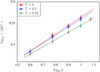
Figure 1: Free-energy change $\Delta F$ vs system size $L$ for $T=0$, $0.2$, and $0.42$. The straight lines are fits of the form $\Delta F\sim aL^{\theta}$.

Table 2: Estimates of the stiffness exponents $\theta$ and $\theta_{\lambda}$ for different temperatures $T$.

$T$	$0$	$0.2$	$0.42$
$\theta$	$0.197(17)$	$0.189(17)$	$0.169(12)$
$\theta_{\lambda}$	—	$0.290(30)$	$0.268(20)$

Next consider the sample stiffness measure $\lambda_{\cal J}$, defined in Eq. (7). Let $G_{L}(\lambda)$ be the cumulative distribution function for $\lambda$. The left panel of Fig. 2 is a log plot of $1-G_{L}(\lambda)$, the complementary cumulative distribution function, for $\lambda$ at $T=0.42$, and sizes $4$ through $12$. The nearly straight line behavior of $\log(1-G_{L}(\lambda))$ is indicative of a nearly exponential tail and suggests a data collapse if $\lambda$ is scaled by a characteristic $\lambda_{\rm char}(L)$ given by the slope of the line. Since the tail is not perfectly straight, we instead define $\lambda_{\rm char}(L)$ in terms of median-like quantities. If the distribution were exactly exponential then $1-G(\lambda)=e^{-\lambda/\lambda_{\rm char}}$ and $1-G(\lambda_{\rm char}\log b)=1/b$ for any $b$. If the distribution is not perfectly exponential, $\lambda_{\rm char}$ depends on $b$ so there is some ambiguity in the definition. We choose $b$ such that $\lambda_{\rm char}$ is obtained from the tail of the distribution but not so far into the tail that the statistics are poor. For $T=0.2$ we choose $b=2$ so $\lambda_{\rm char}$ is defined as the median divided by $\log 2$. For $T=0.42$ we choose $b=10$ to ensure that $\lambda_{\rm char}$ is obtained from the tail of the distribution. The right panels of Figs. 2 and 3 show $1-G_{L}(\lambda/\lambda_{\rm char}(L))$ for $T=0.42$ and $T=0.2$, respectively, and reveal that all of the cumulative distributions collapse onto the same curve when scaled by $\lambda_{\rm char}(L)$.

Figure 4 shows $\lambda_{\rm char}(L)$ vs $\log L$ for $T=0.2$ and $T=0.42$. Since $\lambda_{\rm char}(L)$ is a stiffness measure, we can extract a new stiffness exponent $\theta_{\lambda}$ from a fit to the form,

$$\lambda_{\rm char}(L)\sim aL^{\theta_{\lambda}}.$$ (10)

The values of $\theta_{\lambda}$, given in Table 2, are larger than $\theta$ obtained from the average free energy difference but close to the value, $0.27$, found in Ref. Carter et al. (2002) using aspect ratio scaling. Presumably, the asymptotic values of $\theta$ and $\theta_{\lambda}$ are the same. We prefer the larger value, $\theta_{\lambda}$ because it is obtained from the tail of the stiffness distribution so we believe it reflects the large-size behavior more accurately than the average free energy difference that defines $\theta$. Aspect ratio scaling is an independent way to minimize finite-size effects and it is interesting that these two approaches yield the same answer within error bars.

It seems clear that $\lambda_{\rm char}(L)\to\infty$ as $L\rightarrow\infty$. At least on a coarse scale, the full distribution $G_{L}(\lambda)$ also scales with $\lambda_{\rm char}(L)$. A closer look at $G$ near the head of the distribution for $T=0.42$ shows that the data collapse is not perfect and there are significant finite-size corrections near $\lambda=0$. Figure 5 shows $1-G_{L}(\lambda/\lambda_{\rm char}(L))$ vs $\lambda$ in the region near $\lambda=0$ for $T=0.42$. Note that curves do not collapse perfectly and that $1-G_{L}(\lambda/\lambda_{\rm char}(L))$ appears to be increasing with $L$. Figure 6 is the same plot for $T=0.2$. Because $G_{L}(0)$ is so small for $T=0.2$, the error bars are too large to discern whether there is a trend with $L$. A reasonable hypothesis is that there is an asymptotic $L\rightarrow\infty$ scaling function $G_{\infty}(z)$ where $z=\lambda/\lambda_{\rm char}$ such that $G_{L}(\lambda)\rightarrow G_{\infty}(\lambda/\lambda_{\rm char}(L))$. The straight line behavior of $\log(1-G_{\infty}(z))$ for large $z$ and increasing trend with $L$ for small $z$ suggests that $G_{\infty}(0)=0$ and $G_{\infty}(z)$ is exponential for $z\gg 1$. In more physical terms, if $G_{\infty}(z)$ exists and is zero for $z\rightarrow 0^{+}$, it means that a single boundary condition dominates the TBC ensemble almost surely, i.e., the dominant boundary condition almost always has a much lower free energy than the other seven boundary conditions. A more complicated possibility is that $G_{\infty}(0^{+})>0$. The consequences of these possibilities for the RSB vs two-state pictures are discussed in Sec. VI.

It is noteworthy that for the system sizes accessible to simulations, $\lambda_{\rm char}(L)$ is sufficiently small that the TBC ensemble contains a mixture of several competing boundary conditions for a substantial fraction of samples. The disorder average $I_{L}$ is dominated by these samples and is therefore not characteristic of the large-$L$ behavior when $\lambda_{\rm char}(L)$ is expected to be large. In what follows we circumvent this difficulty by extrapolating first in $\lambda$ and then in $L$, making use of the fact our data contain a relatively large dynamic range in $\lambda$.

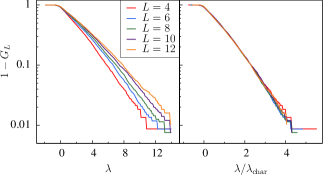
Figure 2: (Left panel) Linear-log plot of $1-G_{L}(\lambda)$ (the complementary cumulative distribution function) vs $\lambda$ for sizes $L=4$ through $12$ at $T=0.42$. (Right panel) $1-G_{L}(\lambda/\lambda_{\rm char}(L))$ vs $\lambda/\lambda_{\rm char}(L)$.

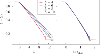
Figure 3: (Left panel) Linear-log plot of $1-G_{L}(\lambda)$ (the complementary cumulative distribution function) vs $\lambda$ for sizes $L=4$ through $10$ at $T=0.2$. (Right panel) $1-G_{L}(\lambda/\lambda_{\rm char}(L))$ vs $\lambda/\lambda_{\rm char}(L)$.

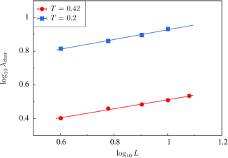
Figure 4: Log-log plot of $\lambda_{\rm char}(L)$ vs $L$ for $T=0.2$ and $T=0.42$. The straight lines represent fits of the form $\lambda_{\rm char}(L)\sim aL^{\theta_{\lambda}}$.

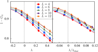
Figure 5: (Left panel) $1-G_{L}(\lambda)$ vs $\lambda$ for system sizes $L=4$ through $12$ at $T=0.42$ in the region near $\lambda=0$. (Right panel) $1-G_{L}(\lambda/\lambda_{\rm char}(L))$ vs $\lambda/\lambda_{\rm char}(L)$. Note that $1-G_{L}(0)$ increases slowly with $L$.

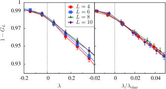
Figure 6: (Left panel) $1-G_{L}(\lambda)$ vs $\lambda$ for system sizes $L=4$ through $10$ at $T=0.2$ in the region near $\lambda=0$. (Right panel) $1-G_{L}(\lambda/\lambda_{\rm char}(L))$ vs $\lambda/\lambda_{\rm char}(L)$.

V.2 Order parameter near $q=0$

Figure 7 shows $I_{L}$, the disorder average of the integrated order parameter distribution with $|q|<0.2$, as a function of size $L$ for temperatures $T=0.2$ and $0.42$, as well as for both PBC and TBC. For both boundary conditions, $I_{L}$ is, within error bars, independent of system size. The results for PBC are identical to those obtained using parallel tempering Monte Carlo Katzgraber et al. (2001); Yucesoy et al. (2012). In fact, in Fig. 8 we show a scatter plot of $I_{\cal J}$ computed both with population annealing and parallel tempering Monte Carlo. The data are strongly correlated and both methods yield the same results within statistical errors.

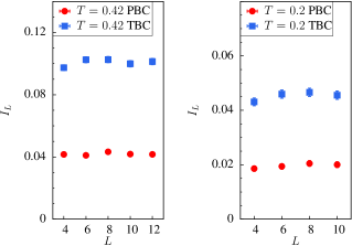
Figure 7: $I_{L}$ vs $L$ for PBC and TBC at temperature $T=0.42$ (left panel) and $T=0.2$ (right panel). The data seem independent of system size, suggesting an RSB interpretation of the data.

The constancy of $I_{L}$ has been taken as strong evidence for the RSB picture because the two-state picture predicts $I_{L}$ should decrease as $L^{-\theta}$. However, in what follows we argue that in TBC ultimately $I_{L}\rightarrow 0$ for very large $L$. On first glance the results for TBC are surprising since $I_{L}^{\rm TBC}$ is larger by more than a factor of two than $I_{L}^{\rm PBC}$. The explanation is that for many samples the TBC ensemble contains several boundary conditions with significant weight and the overlap between spin configurations with different boundary conditions will tend to have small values of $q$ due to the existence of a relative domain wall. We shall return to this important point in Sec. VI.

Figure 8: Log-log scatter plot of $I_{\cal J}$ for PBC for each sample at temperature $T=0.20$ and $L=10$ computed with parallel tempering Monte Carlo (PT, vertical axis) and population annealing Monte Carlo (PA, horizontal line). The data show both methods yields the same result for each sample within statistical errors.

V.3 Order parameter near $q=0$ vs spin stiffness

Figure 9 is a scatter plot showing many of the disorder samples at $T=0.42$ (left panel) and $T=0.2$ (right panel) for all the sizes studied using TBC. Each point on the plot represents a sample $\cal J$. The $x$ coordinate of the point is $\lambda_{\cal J}=\log\left[f_{\cal J}/(1-f_{\cal J})\right]$ and the $y$ coordinate is $I_{\cal J}$. Figure 10 is the same as Fig. 9 but with each system size on a separate plot for $T=0.2$. The qualitative features of the plots are the same for each size although, as described above, the distribution of $\lambda$’s shifts to larger values for larger $L$. These figures together with the behavior of the $\lambda$ distribution constitute the main results of our paper and motivate our conclusion that $I_{\cal J}\rightarrow 0$ almost surely as $L\rightarrow\infty$ in thermal boundary conditions.

Samples $\cal J$ for which $I_{\cal J}$ or $1-f_{\cal J}$ are exactly zero within the precision of the simulations are not shown on these log-log plots since $\log I_{\cal J}=-\infty$ or $\lambda_{\cal J}=\infty$. The fractions of such samples are given in Table 3. Note that actual values of $I_{\cal J}$ or $1-f_{\cal J}$ are are never exactly zero for finite systems; zeros correspond to values smaller than can be represented by the finite population sizes used in the simulations. It is important to note that the trends shown in Fig. 9 continue to hold for the large values of $\lambda$ that are omitted from this figure. Including all sizes, there are $216$ samples with $1-f_{\cal J}=0$ for $T=0.42$ and $2996$ such samples for $T=0.2$. Of these, only seven samples for $T=0.42$ and $38$ for $T=0.2$ are measured to have nonzero values of $I_{\cal J}$. The average value of $I$ for only those samples with $1-f_{\cal J}=0$ are $2.5\times 10^{-8}$ and $10^{-4}$ for $T=0.42$ and $T=0.2$, respectively.

Table 3: Fraction of samples with $I_{\cal J}=0$ and $f_{\cal J}=1$ for different sizes, temperatures, and boundary conditions.

PBC
System size $L$	4	6	8	10	12
Fraction $I_{\cal J}=0\ (T=0.42)$	0.21	0.19	0.16	0.16	0.19
Fraction of $I_{\cal J}=0\ (T=0.2)$	0.60	0.57	0.55	0.54	–
Fraction of $f_{\cal J}=1\ (T=0.42)$	–	–	–	–	–
Fraction of $f_{\cal J}=1\ (T=0.2)$	–	–	–	–	–
TBC
System size $L$	4	6	8	10	12
Fraction $I_{\cal J}=0\ (T=0.42)$	0.05	0.04	0.03	0.03	0.03
Fraction of $I_{\cal J}=0\ (T=0.2)$	0.35	0.33	0.30	0.28	–
Fraction of $f_{\cal J}=1\ (T=0.42)$	0.009	0.009	0.008	0.008	0.010
Fraction of $f_{\cal J}=1\ (T=0.2)$	0.15	0.16	0.15	0.15	–

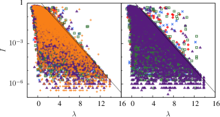
Figure 9: (Color online) Scatter plots showing all disorder realizations for all system sizes at $T=0.42$ (left panel) and $T=0.2$ (right panel). Each point represents a sample $\cal J$ located at $x$ coordinate $\lambda_{\cal J}$ and $y$ coordinate $I_{\cal J}$. Red diamonds represent $L=4$, blue crosses $L=6$, green squares $L=8$, purple triangles $L=10$, and orange plus symbols $L=12$.

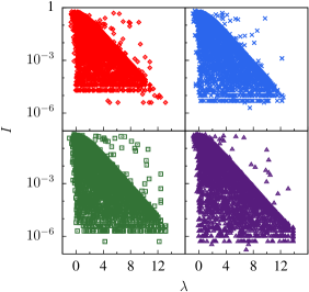
Figure 10: (Color online) Same as Fig. 9 but for each system size in a separate panel and $T=0.2$. Again, red diamonds represent $L=4$, blue crosses $L=6$, green squares $L=8$, and purple triangles $L=10$.

A striking feature of Figs. 9 and 10 is that there is a bounding curve that becomes a straight line for large $\lambda$ with most samples lying below that curve. Why are there two classes of samples, with most samples below the curve and a few above it? We speculate that the samples below the curve have nonzero values of $I_{\cal J}$ as a result of the overlap between spin configurations with different boundary conditions. The contribution to the overlap between different boundary conditions in the TBC ensemble cannot exceed $2f(1-f)$ in the limit $f\rightarrow 1$, so that if this is the primary mechanism producing small overlaps in sample $\cal J$ then $\log I_{\cal J}<(-\lambda_{\cal J}+\log 2$). The straight lines in Fig. 9 are defined by $\log I=(-\lambda+\log 2)$. Thus, for most samples, we believe that the primary contribution to $I_{\cal J}$ comes from the overlap between different boundary conditions. For the rare samples above the bounding curve, the primary contribution to $I_{\cal J}$ must come from small overlaps within the dominant boundary condition.

A second important feature of Figs. 9 and 10 is that the rare samples above the bounding curve have $I_{\cal J}$ roughly uniformly distributed on a logarithmic scale between the bounding curve and $1$. On a linear scale this means that for large $\lambda$ almost all of these samples have small values of $I_{\cal J}$. Let $\rho(x|y)$ be the conditional probability density for $x=I_{\cal J}$ conditioned on $y=\lambda_{\cal J}$. If this distribution is exactly log uniform above the bounding line then the part of the distribution above the line would take the form,

$$\rho(x|y)=\frac{1-w(y)}{xy}\;\;\;\;\;\;\;\mbox{ for }\;\;\;\;\;\;\;x>2\exp(-y),$$ (11)

where $w(y)$ is the fraction samples below the bounding line. Figure 11 shows histograms of $I_{\cal J}$ values of the samples of all sizes that lie above the bounding line for the two temperatures. The position $\alpha$ along the horizontal axis is the scaled logarithmic distance between the bounding line and one. That is, $\alpha_{\cal J}=-\log I_{\cal J}/[\lambda-\log(2)]$ so that zero corresponds to large values, $I_{\cal J}\approx 1$ while one corresponds to $I_{\cal J}$ on the bounding line. For $T=0.2$ the distribution is indeed relatively uniform on a logarithmic scale while for $T=0.42$ it is skewed to a small value of $I$.

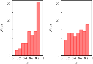
Figure 11: Histogram ${\mathcal{N}}(\alpha)$ for $\alpha_{\cal J}=\log(I_{\cal J})/[-\lambda_{\cal J}+\log(2)]$ for $T=0.42$ (left panel) and $T=0.2$ (right panel). $\alpha=1$ corresponds to the small values of $I$ at the bounding line.

VI Discussion

Three salient features of the data are apparent from Figs. 4, 9, and 11.

1. Typical values of the sample stiffness $\lambda_{\cal J}$ increase with system sizes $L$, as described by $\lambda_{\rm char}(L)$.

2. Most samples have $I_{\cal J}$ less than a bounding curve described by $2e^{-\lambda}$ for large $\lambda$.

3. Samples with $I_{\cal J}$ above the bounding curve have $I_{\cal J}$ distributed more or less uniformly in $\log I$ between the bounding curve and one.

We conjecture that these features hold for arbitrarily large $L$ and all temperatures in the low-temperature phase. Assuming the above statements are asymptotically correct, we can draw some strong conclusions about how $I_{L}$ behaves for sufficiently large $L$ that $\lambda_{\rm char}(L)\gg 1$. Note that these system sizes are far larger than are accessible in our simulations but, given the large dynamic range in $\lambda$ we can extrapolate to these sizes by first extrapolating in $\lambda$. For large $L$, $\lambda_{\cal J}$ is nearly always large according to Statement (I). Furthermore, due to Statements (II) and (III), $I_{\cal J}$ is, almost always small when $\lambda_{\cal J}$ is large. Thus $I_{\cal J}$ is nearly always small when $L$ is large. This conclusion is the main result of our analysis. It is consistent with two-state pictures but not consistent with the RSB picture.

In addition to being consistent with our data, these conjectures are quite plausible. Statement (I) asserts that $\lambda_{\cal J}$ is a measure of sample stiffness and that in the low-temperature phase, almost all samples become stiff for large system sizes. As discussed above, Statement (II) asserts that in TBC large values of $I_{\cal J}$ arise mostly from the overlap between two different boundary conditions. Statement (III) asserts that the free-energy cost of a large excitation in the dominant boundary condition is more or less uniformly distributed between $\lambda/\beta$ and $0$.

We can make the arguments more quantitative using a simple model of how the disorder average $I_{L}$ will behave for large $L$. Let $\rho(x|y)$ be the conditional probability density for $I_{\cal J}=x$ conditioned on $\lambda_{\cal J}=y$. Based on statements (II) and (III) we propose the form,

$$\rho(x|y)=w(y)\delta[x,2\exp(-y)]+\frac{1-w(y)}{xy}\theta[x-2\exp(-y)],$$ (12)

where $w(y)$ is the fraction of samples at fixed $\lambda$ below the bounding curve, and $\theta(x)$ and $\delta(x,y)$ are the Heaviside function and the $\delta$-function, respectively. The first term conservatively places all the samples below the bounding curve on the curve itself. The second term represents the samples above the bounding curve with the conservative assumption that the distribution of $I_{\cal J}$ above the curve is uniform on a log scale as in Eq. (11). For purposes of the following calculation we assume that $w$ is a constant independent of $y$ but the qualitative conclusions do not depend on this assumption. Finally, we assume that the distribution of $\lambda$ obeys a size independent form $G_{\infty}(z)$ for the scaled variable $z=\lambda/\lambda_{\rm char}(L)$. Note that we have assumed that the dependence of $I_{L}$ on $L$ is entirely through $\lambda_{\rm char}(L)$ and that the conditional probability $\rho(x|y)$ is independent of $L$. These assumptions yield an explicit expression for $I_{L}$ as a function of $\lambda_{\rm char}(L)$,

$$I_{L}=\frac{1}{\lambda_{\rm char}(L)}\int_{0}^{\infty}dG_{\infty}(z)\int_{0}^{\infty}dx~{}x\rho(x|z\lambda_{\rm char}(L)).$$ (13)

Plugging in the ansatz of Eq. (12) and an exponential form for the scaled $\lambda$ distribution, $1-G_{\infty}(z)=e^{-z}$, yields a somewhat complex expression involving exponential integrals whose asymptotic large $\lambda$ behavior is,

$$I_{L}\sim\frac{1}{\lambda_{\rm char}(L)}\left[2w+(1-w)\log(\lambda_{\rm char}(L))\right].$$ (14)

Using Eq. (10) and assuming that asymptotically $\theta_{\lambda}=\theta$, we recover the prediction of the two-state picture that $I_{L}\sim L^{-\theta}$, however, with a logarithmic correction that arises from the assumption of a log-uniform distribution for $I_{\cal J}$.

While the above assumptions lead to an explicit asymptotic expression for $I_{L}$ as a function $L$, this expression should not be taken too seriously. However, the qualitative conclusion that $I_{\cal J}\rightarrow 0$ for almost all samples as $L\rightarrow\infty$ is robust and depends only on the asymptotic validity of statements (I) — (III) above.

Given that $\lambda_{\rm char}(L)$ is increasing with $L$ and that $I$ decreases with increasing $\lambda$, why is $I_{L}$ nearly constant for the sizes studied in our TBC simulations of the 3D EA model? We believe this conundrum can be explained, at least in part, by the fact that the main contribution to $I_{L}$ comes from samples with small values of $\lambda$. For $T=0.2$, more than half the contribution to $I_{L}$ comes from samples with $\lambda<1$ and more than $80\%$ from $\lambda<2$, and these fractions are even higher for $T=0.42$. The head of the $\lambda$ distribution, has very little dependence on $L$, as can be seen in Figs. 2 and 3. Furthermore, the bounding curves in Fig. 9 are nearly flat in the small $\lambda$ region. Thus several effects come into play in keeping $I_{L}$ nearly independent of $L$. First, the main contribution to $I_{L}$ is from samples with small stiffness. Second, the fraction of samples with small stiffness decreases by only a small amount for the sizes studied and, finally, $I$ does not depend much on $\lambda$ for small $\lambda$. One would have to go to much larger sizes before $I_{L}$ would decrease according to the predicted asymptotic power law $L^{-\theta}$.

In the foregoing, we have assumed that $G_{L}(0)\rightarrow 0$ as $L\rightarrow\infty$ or, equivalently, if $G_{\infty}(z)$ exists, $G_{\infty}(0^{+})=0$. We now consider the consequences of an alternate assumption that $\lambda_{\rm char}(L)\rightarrow\infty$ and $G_{\infty}(z)$ exists but $G_{\infty}(0^{+})>0$. This possibility cannot be ruled out by the data although if it holds, it appears that $G_{\infty}(0^{+})$ is quite small. In physical terms $G_{\infty}(0^{+})>0$ means that even for very large sizes, a fraction $G_{\infty}(0^{+})$ of samples has a mixed ensemble of boundary conditions in TBC while the remaining samples have only a single boundary condition in the TBC ensemble. This scenario would imply that the 3D EA model in TBC is divided into two classes of disorder realizations, one of which, with weight $(1-G_{\infty}(0^{+}))$, has $I_{L}=0$ and the other, with weight $G_{\infty}(0^{+})$, has $I_{L}>0$. This possibility seems unlikely but is not contradicted by the data. It has no straightforward explanation in either two-state or RSB pictures.

Our hypothesis is that thermal boundary conditions and periodic boundary conditions have the same behavior in the limit of large system sizes. We use thermal boundary conditions as a tool to improve the extrapolation to large system sizes from the very small system sizes accessible in simulations. It is known that coupling dependent boundary conditions are not equivalent to periodic boundary conditions and are not suitable for understanding properties of the spin glass phase because they could be used to select a single pure state even if coupling independent boundary conditions admit many pure states. The status of thermal boundary conditions with regard to coupling dependence is not clear. On the one hand, the TBC ensemble contains different mixtures of boundary conditions for different choices of couplings. On the other hand, the particular mixture of the 8 boundary conditions is chosen by the system itself and is not imposed externally. As discussed in Sec. II.2, our intuition is that TBC minimizes finite size effects rather than introducing spurious physics but this question requires further investigation. In any case, we have provided compelling evidence that the 3D EA model in thermal boundary conditions is best described by a picture with a single pair of pure states in each finite volume.

VII Summary

We have introduced two techniques with the aim of extrapolating to the large system-size behavior of finite-dimensional spin glasses at low temperature. First, we use thermal boundary conditions to minimize the effect of domain walls induced by boundary conditions. Second, we use a natural measure of sample stiffness defined within thermal boundary conditions and extrapolate to large values of the sample stiffness. By noting that the sample stiffness increases with system size we then obtain an extrapolation in system size. The dynamic range in sample stiffness in the data is sufficiently large that a qualitative extrapolation is readily apparent. The conclusion is that nearly all large samples will have essentially no weight in the overlap distribution near zero overlap. The analysis also explains why this qualitative behavior cannot be seen using a direct extrapolation in system size for the small sizes studied. Our conclusions are consistent with two-state pictures but are inconsistent with the mean field, replica symmetry breaking picture.

Our results hold for thermal boundary conditions. We believe that thermal boundary conditions are equivalent to other coupling independent boundary conditions so that our conclusions about the infinite volume limit also apply to the more familiar periodic boundary conditions. However, it is important to investigate the equivalence of thermal and periodic boundary conditions.

Our numerical simulations used population annealing. This Monte Carlo algorithm has not been used before for large-scale studies in statistical physics. We found that it is an effective computational tool with several advantages over parallel tempering, the standard computational method in the field. We believe that population annealing will be useful for other hard problems in statistical physics and related fields. Similarly, thermal boundary conditions and extrapolating in sample stiffness are general methods that should be useful in studying other finite-dimensional disordered systems.