Meteorological data for the astronomical site at Dome A, Antarctica

Abstract

We present an analysis of the meteorological data collected at Dome A, Antarctica by the Kunlun Automated Weather Station, including temperatures and wind speeds at eight elevations above the snow surface between 0$\,\rm m$ and 14.5$\,\rm m$. The average temperatures at 2$\,\rm m$ and 14.5$\,\rm m$ are $-54^{\circ}$C and $-46^{\circ}$C, respectively. We find that a strong temperature inversion existed at all heights for more than 70% of the time, and the temperature inversion typically lasts longer than 25 hours, indicating an extremely stable atmosphere. The temperature gradient is larger at lower elevations than higher elevations. The average wind speed was 1.5$\,\rm m/s$ at 4$\,\rm m$ elevation. We find that the temperature inversion is stronger when the wind speed is lower and the temperature gradient decreases sharply at a specific wind speed for each elevation. The strong temperature inversion and low wind speed results in a shallow and stable boundary layer with weak atmospheric turbulence above it, suggesting that Dome A should be an excellent site for astronomical observations. All the data from the weather station are available for download.

1 Introduction

Dome A—the highest location on the Antarctic Plateau at an elevation of 4,089m—has long been considered to be an excellent site for astronomical observations over a broad range of the electromagnetic spectrum (e.g., Gillingham 1991, Marks 2002, Burton 2010, and references therein). Dome A’s advantages include extremely low temperatures, an extremely dry atmosphere (Sims et al. 2012), low wind speed, and long periods of continuous cloud-free nighttime.

Other sites in Antarctica, such as the South Pole itself, Dome C, and Dome Fuji, are also promising, and have been extensively studied over many years with a variety of instruments. Astronomers are particularly interested in the layer within tens or hundreds of meters of the surface over the Antarctic plateau since a number of studies (e.g., Marks et al. 1999, Lawrence et al. 2004) have shown that the transition to the free atmosphere occurs within this height range, as opposed to 1–2$\,\rm km$ from typical observatory sites at temperate latitudes.

At the South Pole, Marks et al. (1996) used microthermal sensors on a 27$\,\rm m$ mast to measure the turbulence in the lowest part of the boundary layer at South Pole. Marks et al. (1999) extended the altitude coverage by using balloon-borne microthermals to estimate a free-atmosphere seeing component of 0.37$\,{}^{\prime\prime}$  above a boundary layer with an average thickness of $\sim$220$\,\rm m$. Travouillon et al. (2003) confirmed these results using a sonic radar able to reach heights of 890$\,\rm m$ above the surface, and derived a ground-based average seeing of 1.73$\,{}^{\prime\prime}$, dropping to 0.37$\,{}^{\prime\prime}$ above 300$\,\rm m$.

At Dome C, Lawrence et al. (2004) used a MASS-DIMM instrument and a SODAR to measure a median free atmospheric seeing of 0.23$\,{}^{\prime\prime}$ above a boundary layer that was less than 30$\,\rm m$ high. Aristidi et al. (2005) analyzed two decades of temperature and wind speed data from an automated weather station, and four summers of measurements with balloon-borne sondes. Trinquet et al. (2008) used balloon-borne measurements to find that the median value of the boundary layer height at Dome C is 33$\,\rm m$.

At Dome Fuji, astronomical seeing at times below 0.2$\,{}^{\prime\prime}$ has been reported from a DIMM instrument 11$\,\rm m$ above the snow surface (Okita et al. 2013).

Dome A was first visited by a Chinese Antarctica Research Expedition (CHINARE) team in 2005, so opportunities for studying the site conditions have not existed for as long as for the other sites in Antarctica. Following the repeated visits in recent years by CHINARE teams, and the construction of the Kunlun Station at Dome A in 2009, several site-testing experiments have been installed (e.g., Yang et al. 2009) and encouraging results have been reported (e.g., Yang et al. 2010). For example, using data from a sonic radar, Bonner et al. (2010) found that the median boundary layer thickness at Dome A between February and August in 2009 was only 13.9$\,\rm m$, considerably lower than the median value of 33$\,\rm m$ at Dome C (Trinquet et al. 2008) and 200–300$\,\rm m$ at South Pole (Travouillon et al. 2003).

Missing up until now has been a detailed analysis of the meteorological conditions at Dome A from mast-based instruments. Such measurements can give direct information on the atmospheric turbulence and wind speed in the boundary layer, and are relevant to the operating environment of future telescopes, and the performance of adaptive optics systems (Aristidi et al. 2005). In this article, we present the first results from analyzing the weather data collected from the Kunlun Automated Weather Station (KL-AWS) at Dome A. Data acquisition and reduction are described in §2. A statistical analysis of temperature and wind speed data are presented in §3. Finally, a discussion is given in §4.

2 Data acquisition and reduction

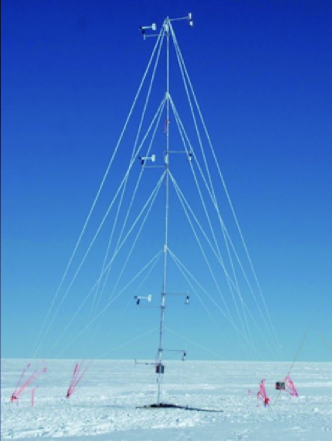
Figure 1: The Kunlun Automated Weather Station (KL-AWS) installed at Dome A in January 2011. The propeller anemometers at 2$\,\rm m$, 4$\,\rm m$, 9$\,\rm m$ and 14.5$\,\rm m$ are clearly visible.

KL-AWS was installed in 2011 January by the 27th CHINARE team (see Fig. 1) at Dome A at the location 80^∘ 25^′ 03$\,{}^{\prime\prime}$ S, 77^∘ 05^′ 32$\,{}^{\prime\prime}$ E. KL-AWS consists of a 15$\,\rm m$ mast equipped with nine Young 4-wire 41342 temperature sensors at heights of $-$1$\,\rm m$, 0$\,\rm m$, 1$\,\rm m$, 2$\,\rm m$, 4$\,\rm m$, 6$\,\rm m$, 9.5$\,\rm m$, 12$\,\rm m$ and 14.5$\,\rm m$, four Young Wind Monitor-AQ model 05305V propeller anemometers at heights of 2$\,\rm m$, 4$\,\rm m$, 9$\,\rm m$ and 14.5$\,\rm m$ to measure both wind speed and direction, and one Young 61302V barometer at 1$\,\rm m$. The manufacturer’s specified absolute measurement accuracy of the instruments is: temperature $0.32^{\circ}$C, wind speed 0.2$\,\rm m/s$, and wind direction $0.5^{\circ}$ plus installation offset. Originally, the mast was planned to have four Young 85000 2D sonic anemometers, but an electrical fault prevented their operation. The anemometer at 2$\,\rm m$ did not acquire data for unknown reasons. KL-AWS was powered by PLATO, an automated observatory (Lawrence et al. 2008), and it was connected to the supervisor computers in PLATO’s instrument module. KL-AWS was placed 30$\,\rm m$ south of PLATO to minimize any influence from nearby structures. KL-AWS acquired data from all sensors once every 36 seconds and stored the data on the hard disks of the supervisor computer. The data were sent back in real-time every 20 minutes through the Iridium satellite network in order to assist with monitoring and operating the other experiments on site.

KL-AWS began operation on 2011 January 17 and ran continuously for a year apart from a 20 day gap beginning on 2011 August 3 due to a computer script inadvertently stopping. The sampling rate was $1/36$Hz up until 2011 August 3, and $1/60$Hz from 2011 August 23. Since then, all the temperature sensors and the barometer were still working but the anemometer at 14.5$\,\rm m$ was never recovered, and other two anemometers at 4$\,\rm m$ and 9$\,\rm m$ were recovered on October 13. On 2012 January 18, KL-AWS ceased operation, possibly as a result of damage to the power and data cables connecting it to PLATO.

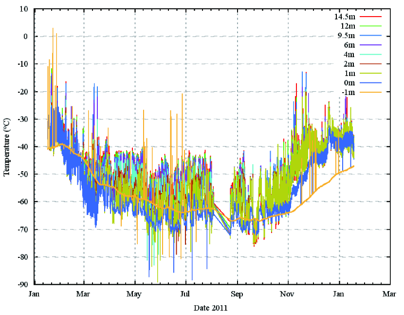
Figure 2: Temperatures at nine heights, from 1$\,\rm m$ under the snow surface to 14.5$\,\rm m$ above the snow. The smoothed data (see §2) are shown in this figure. The raw data are available for download (see §4).

Fig. 2 shows all the temperature data collected by KL-AWS.

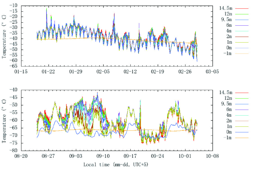
Figure 3: Temperatures recorded during the first 40 days of KL-AWS operation (top panel) in 2011 and 40 days following a restart of KL-AWS on 2011 August 23 (bottom panel). The changes in the temperature distribution from 2011 September 16 are believed to have been caused by the collapse of the upper part of the mast. This figure shows smoothed data (see §2).

When the CHINARE expedition revisited Dome A at the beginning of 2012 it was found that the top section of the weather tower had bent over and almost touched the ground. From looking at the data we determined that the tower likely failed on 2011 September 16 (see Fig. 3). Before that date there were often large temperature differences between the sensors, but after September 16 the higher sensors showed no differences. Unless otherwise stated, this paper restricts itself to the continuous period of data up until 2011 August 3.

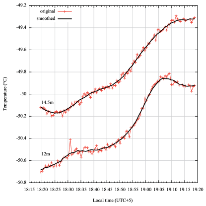
Figure 4: An example of temperature data smoothing for the 14.5$\,\rm m$ and 12$\,\rm m$ sensors for a one hour period on May 15, 2011. Note that the reproducibility of individual measurements on these timescales is much better than the absolute sensor accuracy of $0.32^{\circ}C$.

To reduce the short-term fluctuations in the data, we have smoothed the temperature data by a boxcar of 10 adjacent data points. Fig. 4 shows an example of the results where the short-term fluctuations are removed while the temperature trends remains. All the following analyses are based on the smoothed temperature data.

3 Results

3.1 Temperature and Temperature Difference

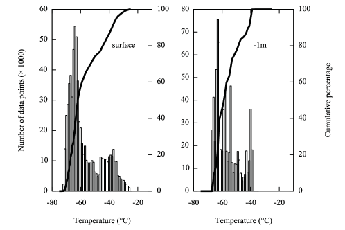
Figure 5: Histograms and cumulative distributions (solid lines) of the temperature at the surface level and 1$\,\rm m$ under the snow surface during 2011.

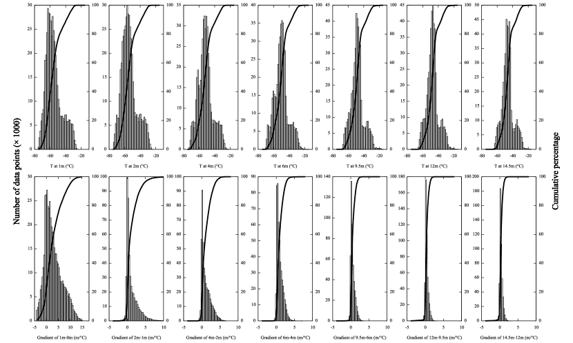
Figure 6: Histograms and cumulative distributions (solid lines) of the temperatures at 1$\,\rm m$, 2$\,\rm m$, 4$\,\rm m$, 6$\,\rm m$, 9$\,\rm m$, 12$\,\rm m$ and 14.5$\,\rm m$ during 2011, and the temperature gradients between every two adjacent levels.

Using data over the entire year, we show the temperature distributions at snow surface level and at $-1$$\,\rm m$ (1 meter below surface) in Fig. 5. As expected, the snow temperature at $-1$$\,\rm m$ has a much smaller range than the air temperature. Due to snow accumulation, we believe the sensor at the snow surface level was buried under snow later in the year and could not provide accurate air temperature measurements. This can be seen clearly in Fig. 3 when the surface temperature line (blue) becomes very smooth in the lower panel. We note the temperature distribution of $-1$$\,\rm m$ shows multiple spikes in the right panel of Fig. 5 and they are real. By investigating the data, we find that the temperature at $-1$$\,\rm m$ varied little around some values for considerable long periods, making such isolated spikes. The temperature distributions at the other heights are shown in Fig. 6 with all data up to 2011 August 3. They all show a single peak distribution.

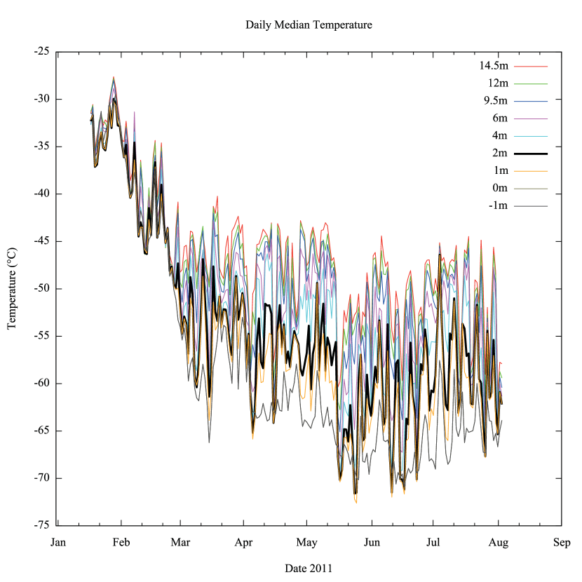
Figure 7: Daily median temperatures during 2011. The bold black line is the temperature at 2$\,\rm m$.

We plot the daily median temperature in Fig. 7 to show the long-term trend which follows the seasonal pattern. The daily median temperature at 2$\,\rm m$ was $\sim-35^{\circ}$C in January, went down rapidly to $\sim-60^{\circ}$C in April, and was as low as $\sim-70^{\circ}$C during the dark winter before it slowly rose again. Compared with that of South Pole, we find that there is no significant difference in monthly median temperature between South Pole and Dome A (see Fig. 2 in Hudson and Brandt 2005). The trend of the daily median temperature is also similar to that at the South Pole.

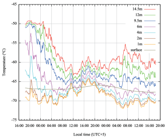
Figure 8: Temperatures at different heights between 2011 May 15 and 2011 May 17. A positive temperature gradient existed as low as 1$\,\rm m$ and lasted for more than two days at all levels. This is indicative of very low atmospheric turbulence.

Because of the radiatively-cooled snow surface, it is not surprising that there is strong temperature inversion just above the snow surface of Dome A. Fig 8 shows a good example of the temperature inversion at different heights. We define the temperature differences at 1$\,\rm m$, 2$\,\rm m$, 4$\,\rm m$, 6$\,\rm m$, 9.5$\,\rm m$, 12.5$\,\rm m$ and 14.5$\,\rm m$ as the temperature at the corresponding height minus the temperature at the adjacent lower height. For example, $\Delta T(2\hbox{\rm m})=T(2\hbox{\rm m})-T(1\hbox{\rm m})$. We then calculate the temperature gradients (in ^∘C/m) at different heights and their distributions are are shown in Fig. 6. The distributions are relatively narrow except for the one involving $\Delta T(1m)$, since the surface temperature that did not always measure the air temperature as explained in §3.1. For all other heights, the distributions increase dramatically from negative values to a positive peak and go down relatively slowly with a tail. The temperature gradients are smaller at higher elevations. The existence of the positive temperature gradients indicates strong temperature inversion at all layers.

To compare the temperatures at two levels spanning more than 10$\,\rm m$ in height, Hudson and Brandt (2005) found at South Pole that for 99.9% of the time there was a positive temperature difference between 13$\,\rm m$ and 2$\,\rm m$. We found the same for our data at Dome A between 12$\,\rm m$ and 2$\,\rm m$. However, the median temperature difference at Dome A was $6.9^{\circ}$C, which is much larger than the difference of $1.1^{\circ}$C at South Pole. This shows that the strength of the temperature inversion at Dome A is much greater than that at South Pole.

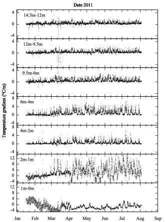
Figure 9: The temperature gradient between 2011 January and August at all levels. The temperature gradients were calculated from the smoothed data (see §2). And the data points were down-sampled by 100 for clarity.

We plot the temperature gradients at all levels between 2011 January and August in Fig. 9. This figure shows that most of the large negative temperature gradients happened during January and February while most of the large positive gradients happened in the wintertime. Higher layers tend to have smaller temperature gradients than lower layers as also seen in Fig. 6.

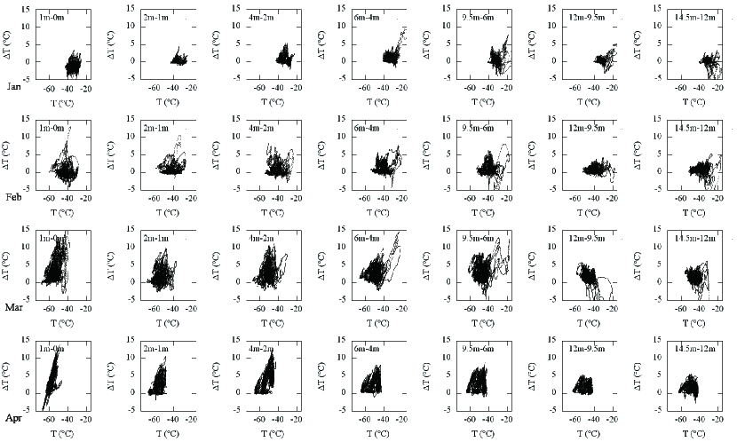
Figure 10: Temperature difference vs. temperature in 2011 January, February, March and April.

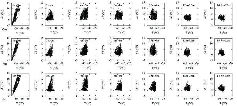
Figure 11: Temperature difference vs. temperature in 2011 May, June and July.

We also investigated whether the temperature inversion depends on the temperature or season. Figs. 10 and 11 show the temperature difference and temperature for different months during 2011. It is clearly seen that most of the largest positive temperature differences (e.g. $>5^{\circ}$C) occurred when the temperature was between $-45^{\circ}$C and $-65^{\circ}$C. The strong correlations between $\Delta T$ and $T$ at 1$\,\rm m$ for later months are not real and are again caused by the snow buried sensor at 0$\,\rm m$ measuring the snow temperature, which did not vary as much as the air temperature. The other plausible correlations for 2$\,\rm m$ and 4$\,\rm m$ after March could be real, suggesting that at lower layers a larger temperature inversion occurred at higher temperatures. There is a strong trend that after March, at 4$\,\rm m$, 6$\,\rm m$, and 9$\,\rm m$, the temperature differences are almost all positive, indicating long durations of temperature inversion.

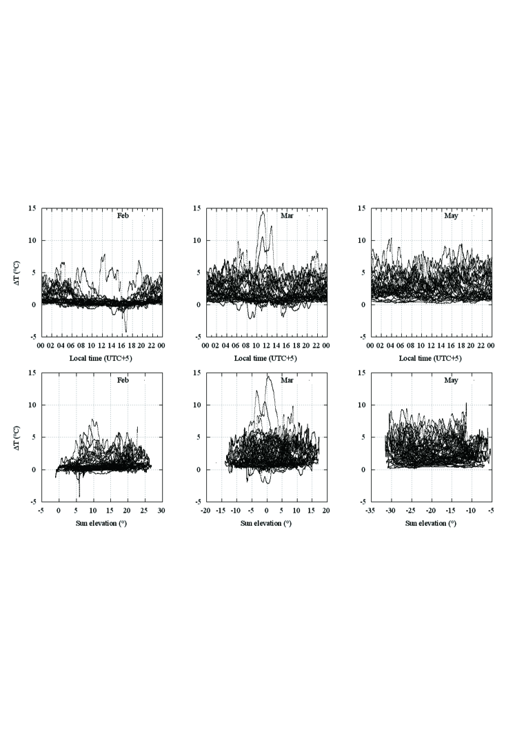
Figure 12: Temperature difference between 6$\,\rm m$ and 4$\,\rm m$ folded into a day during February, March, and May (top) and the same temperature difference vs. solar elevation (bottom).

Although the daily temperature obviously varies with the elevation of the Sun in the summer season as seen in the top panel of Fig. 3, we found that the temperature difference in a day has little relationship with the Sun. In Fig. 12 we fold the temperature difference at 6$\,\rm m$ into one day for February, March and May, and also plot the temperature difference against the solar elevation. In February of 2011, the temperature difference at 6$\,\rm m$ seems to be larger at night and seems to be related to the Sun, but in March when the Sun still rises and sets at Dome A, we do not find a preferable time for larger temperature differences and there is no evidence of correlation between $\Delta T$ and solar elevation.

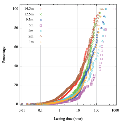
Figure 13: Cumulative distributions of the duration of the temperature inversion (defined as a positive temperature difference larger than $0.14^{\circ}$C) for all heights.

As an indicator of the stability of the atmosphere, we are mostly concerned with how long a temperature inversion lasts. We show a clear example of two days’ data in mid May, 2011 in Fig. 8 where a temperature inversion exists at all heights. We evaluated the temperature inversion (i.e., temperature difference) at each height with respect to the temperature sensor immediately below. To evaluate the duration of a temperature inversion at all heights, we need to define a real temperature difference quantitatively. While the temperature sensors have a specified absolute accuracy of $0.32^{\circ}$C, our data show that the variation in consecutive measurements is much smaller than this (see Fig. 4). We have subtracted the smoothed data from the original data and calculated the standard deviation as $\sigma=0.033^{\circ}$C. Therefore, we set a $3\sigma$ temperature difference threshold of $0.14^{\circ}$C, above which we regard it as a real temperature inversion rather than random measurement error. We choose all the temperature difference data points larger than $0.14^{\circ}$C, and counted how long the inversion lasted. The results are shown in Fig. 13 and Table 1. A temperature inversion existed more than 70% of the time at all heights, and up to 95% at a height of 6$\,\rm m$. We note that when a temperature inversion occurred, it lasted at least 25 hours for more than $\sim$40% of the time at all heights and up to 78% at 6$\,\rm m$. For less than 10% of the time, the temperature inversion lasted under 1 hour.

We also note that the median duration of the temperature inversion increased from 2$\,\rm m$ to 6$\,\rm m$ and then decreased with height. There are two possible reasons for this trend. One is that the air turbulence is stronger at the lower elevation, the other is that sudden strong wind can destroy the temperature inversion at higher elevations (see the next subsection for wind speed statistics).

3.2 Wind speed and direction

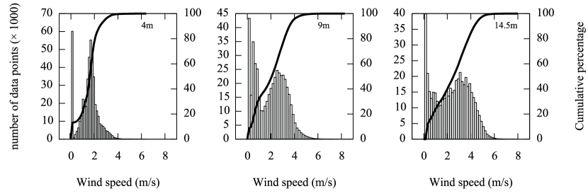
Figure 14: Wind speed histograms and cumulative distributions (solid lines) at 4$\,\rm m$, 9$\,\rm m$ and 14.5$\,\rm m$ during 2011.

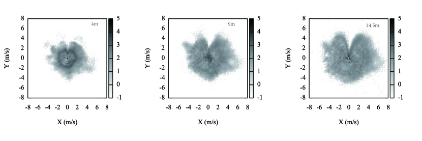
Figure 15: The wind rose density at three heights during 2011. North is up. The gaps are caused by the weather mast which blocked the wind from the north direction. The grey scale is the logarithm of the number of data points per pixel. The obvious darker ring in the 4m plot corresponds to the dominant wind speed around about 1.7$\,\rm m/s$ (see Fig. 14) of random directions. Similar patterns also exist in the other two plots, but not as obvious.

The distributions and cumulative statistics for the wind speed at three heights are shown in Fig. 14. The peak at 0$\,\rm m/s$, accounting for about 10% of the time, simply means there was no wind, or the wind speed was too low to be detected by the sensors, or the sensors got stuck (see below). At 4$\,\rm m$, the wind speed was lower than 1.5$\,\rm m/s$ for half of the time, and seldom reached 4$\,\rm m/s$. The wind speed increases with height above the snow. At 9$\,\rm m$ and 14.5$\,\rm m$, the median wind speeds are 2.0$\,\rm m/s$ and 2.4$\,\rm m/s$, respectively, and could often reach 4$\,\rm m/s$. This can also be clearly seen in the wind rose plots (Fig. 15). We notice that there is no dominant wind direction for all three heights. The obvious gaps in the wind roses are caused by the mast of KL-AWS which blocked wind in that direction.

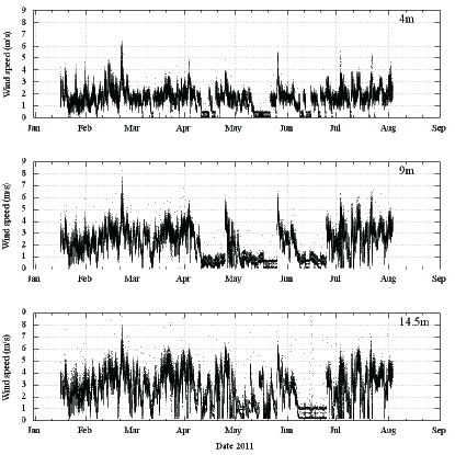
Figure 16: Wind speed during 2011 at three heights. Unsmoothed raw data are shown in this figure.

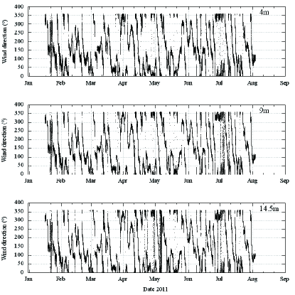
Figure 17: Wind direction during 2011 at three heights. Unsmoothed raw data are shown in this figure.

We have shown the wind speed and direction between January and August in Fig. 16 and Fig. 17, and noticed that when there is virtually no wind, it was mostly during the polar night when the Sun never rose. However, for some extended periods during April to June, the wind speeds were flat in the plots and were 0$\,\rm m/s$ or very low. This makes us to worry that it is possible that the propellers of the anemometers got stuck sometimes at low temperatures. Fig. 17 shows again that the wind directions are random and they are synchronized very well at the three heights.

We have compared the average wind speeds at Dome A, Dome C, and the South Pole in Table 2 and find that the horizontal wind speed at Dome A at 4$\,\rm m$ was only 1.5$\,\rm m/s$, much smaller than the ground wind speed of 2.9$\,\rm m/s$ at Dome C and 5.5$\,\rm m/s$ at the South Pole.

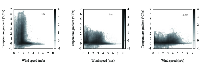
Figure 18: Wind speed against temperature gradient at the corresponding height. The grey scale is the logarithm of the number of data points per pixel. The vertical structures in the plots correspond to the real distribution of the data points in Fig. 14.

In order to investigate whether the temperature gradient is related to wind speed, we plot the wind speeds at 4$\,\rm m$, 9$\,\rm m$ and 14.5$\,\rm m$ against temperature gradients at 4$\,\rm m$, 9.5$\,\rm m$ and 14.5$\,\rm m$ respectively in Fig. 18. Stronger temperature inversion always occurred when the wind speed was lower. When the wind speed is higher than 2.5$\,\rm m/s$ at 4$\,\rm m$, the temperature gradient was never larger than $0.7^{\circ}$C/m. We also see the same trends at 9$\,\rm m$ and 14.5$\,\rm m$, but with different specific wind speeds of 4.1$\,\rm m/s$ and 5.3$\,\rm m/s$, respectively. It therefore seems that at the higher elevations, the positive temperature gradients are smaller, but more resistant to wind.

3.3 Air pressure

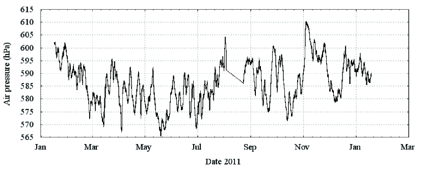
Figure 19: Air pressure during 2011. The raw data for the entire year are shown in this figure. Note that the barometric data should not be influenced by the collapse of the upper part of the mast in September.

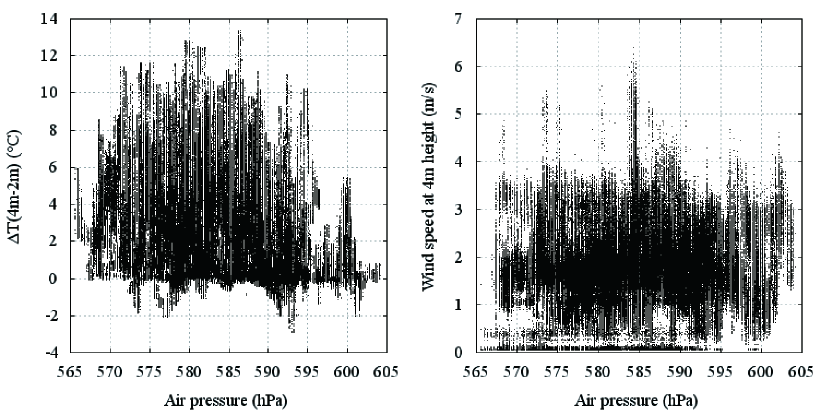
Figure 21: Temperature difference between the 2$\,\rm m$ and 4$\,\rm m$ heights (left panel) and wind speed at 4$\,\rm m$ (right panel) versus air pressure during 2011.

The barometer at the height of 1$\,\rm m$  worked correctly for the entire year. Fig. 19 and 20 shows the data and the distribution. The average air pressure at Dome A was 586 hPa with a standard deviation of 8 hPa. We do not find any clear relationships between the air pressure and the temperature difference or wind speed at 4$\,\rm m$ (Fig. 21).

4 Conclusion and discussion

We have analyzed the weather data collected from KL-AWS at Dome A during 2011. The average temperature between January and July was $-54^{\circ}$C at 2$\,\rm m$ and $-46^{\circ}$C at 14.5$\,\rm m$. We have found that there is usually a strong temperature inversion at all the heights above the ground. The temperature inversion, defined here as a positive temperature difference larger than $0.14^{\circ}$C, existed more than 70% of the time at all heights and up to 95% at 6$\,\rm m$. Such inversions lasted longer than 25 hours for more than about 40% of the time at all heights, and almost 80% of the time at 6$\,\rm m$. Most largest negative temperature differences (no inversion) occurred during January and February and most strong temperature inversion occurred when the temperature fell between $-65^{\circ}$C and $-45^{\circ}$C.

The average wind speed at 4$\,\rm m$ is 1.5$\,\rm m/s$, which may be the lowest reported from any site on earth. The wind speed at higher elevation is slightly stronger. We also notice that for $\sim 10\%$ of the time there is almost no wind or the wind speed was too low to be detected by the sensors, this usually happens during the dark polar night. However, there also seems to be evidence that the wind speed sensors might have been stuck sometimes at low temperatures. The wind on the Antarctic continent is dominated by katabatic winds, therefore the wind speed should be very small and the wind direction should be random above the highest point (Dome A). Hudson and Brandt (2005) found that the strongest temperature inversion often happened with a 3–5$\,\rm m/s$ wind at the South Pole, but we find that strong temperature inversion happens when the wind speed is low, such as less than 2.5$\,\rm m/s$ for the height of 4$\,\rm m$; when the wind speed is higher than 2.5$\,\rm m/s$ the temperature gradient decreases sharply.

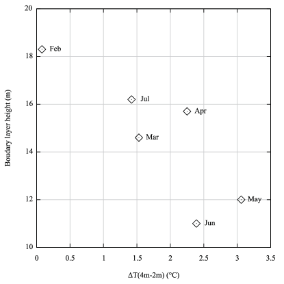
Figure 22: Monthly median boundary layer height during 2009 (Bonner et al. 2010) versus the monthly median temperature difference between heights of 2$\,\rm m$ and 4$\,\rm m$ during 2011.

It has been known for a long time that the surface of the Antarctic plateau is prone to temperature inversions due to radiative cooling of ice, and hence a lower air temperature near the surface. As Basu and Porté-Agel (2006) pointed out, whenever a temperature inversion exists, turbulence is generated by shear and destroyed by negative buoyancy and viscosity. Competition between shear and buoyancy weakens turbulence and results in a shallower boundary layer. We list the monthly median boundary layer heights of Dome A in 2009 (Bonner et al. 2010) and the monthly median temperature difference at 4$\,\rm m$ during 2011 in Table 3 and compared them in Fig. 22. If average conditions were similar between 2009 and 2011, this indicates, as expected, that stronger temperature inversions favor a thinner boundary layer, with the lowest in May and June.

The strong temperature inversion and low wind speed at Dome A both produce a very stable atmosphere and a stable boundary layer with little convection, especially in winter. When the temperature inversion happens as low as 2$\,\rm m$, we expect the boundary layer can be much lower too. Above the shallow boundary layer, we can reach the free atmosphere where the seeing will be good for astronomical observations. In other words, there will be periods when even telescopes that are very close to the ground will experience free-atmosphere seeing approaching 0.25$\,{}^{\prime\prime}$.

We have demonstrated that the weather data collected by KL-AWS at different heights are very useful to characterize the stability of the near-ground atmosphere at Dome A and can provide insights for evaluating the site for astronomical observations. We plan to continue the experiment with a new weather tower and monitor the site for at least 2–3 years so that we can have better statistics and understanding of the site.

The data from KL-AWS are available in raw form at http://aag.bao.ac.cn/weather/downloads/ and as plots at http://aag.bao.ac.cn/weather/plot_en.php

Table 1: Cumulative percentage of the duration of temperature inversion

Height	$>25$ hours	$>10$ hours	Total
1$\,\rm m$	55	66	75
2$\,\rm m$	39	51	71
4$\,\rm m$	64	73	84
6$\,\rm m$	78	89	95
9.5$\,\rm m$	59	76	85
12$\,\rm m$	57	73	86
14.5$\,\rm m$	41	64	85

Table 2: Average wind speed at Dome A, Dome C and the South Pole.

Site	Wind speed ($\,\rm m/s$)	Reference
Dome A (4$\,\rm m$)	$1.5$	This paper
Dome C (3.3$\,\rm m$)	$2.9$	Aristidi et al. (2005)
South Pole (2$\,\rm m$)	$5.5$	Mefford (2004)

Table 3: Dome A monthly median boundary layer height of 2009 (Bonner et al. 2010) and monthly median temperature difference of 2011 between 4$\,\rm m$ and 2$\,\rm m$.

Month	$\Delta T$ (4$\,\rm m$$-$2$\,\rm m$)	Boundary layer height
	∘C	m
January	$0.18$	$\cdots$
February	$0.08$	$18.3$
March	$1.53$	$14.6$
April	$2.25$	$15.7$
May	$3.06$	$12.0$
June	$2.39$	$11.0$
July	$1.42$	$16.2$
August	$\cdots$	$10.2$

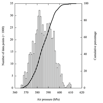
Figure 20: Air pressure histogram and cumulative distribution (solid line) during 2011.

References

- Aristidi et al. (2005) Aristidi, E., Agabi, K., Fossat, E., Vernin, J., Travouillon, T., Lawrence, J.S., Meyer, C., Storey, J. W. V., Halter, B., Roth, W. L., & Walden, V. 2005, A&A, 430, 739.
- Basu & Porté-Agel (2006) Basu, S., & Porté-Agel, F. 2006, J. Atmos. Sci., 63, 2074.
- Bonner et al. (2010) Bonner, C. S., Ashley, M. C. B., Cui, X., Feng, L., Gong, X., Lawrence, J. S., Luong-Van, D. M., Shang, Z., Storey, J. W. V., Wang, L., Yang, H., Yang, J., Zhou, X., & Zhu, Z., 2010, PASP, 122, 1122.
- Burton (2010) Burton, M. G., 2010, A&A Rev., 18, 417.
- Gillingham (1991) Gillingham, P.R., 1991, Proc. Astron. Soc. Australia, 9, 55.
- Hudson & Brandt (2005) Hudson, Stephen R., & Brandt, Richard E., 2005, J. Clim., 18, 1673.
- Lawrence et al. (2004) Lawrence, J. S., Ashley, M. C. B., Tokovinin, A., & Travouillon, T., 2004, Nature, 431, 278.
- Lawrence et al. (2008) Lawrence et al., 2008, Proc. SPIE, 7012, 701227.
- Marks et al. (1996) Marks, R. D., Vernin, J., Azouit, M., Briggs, J. W., Burton, M. G., Ashley, M. C. B., and Manigault, J.-F., 1996, A&AS, 118, 385.
- Marks et al. (1999) Marks, R., Vernin, J., Azouit, M., Manigault, J. F., & Clevelin, C., 1999, A&AS, 134, 161.
- Marks (2002) Marks, R. D., 2002, A&A, 385, 238.
- Mefford (2004) Mefford, T., 2004, NOAA CMDL, http://www.cmdl.noaa.gov.
- Okita (2013) Okita, H., Ichikawa, T., Ashley, M. C. B., Takato, N., & Motoyama, H., 2013, A&A, 554, L5.
- Sims et al. (2012) Sims, G., Ashley, M. C. B., Cui, X., Everett, J. R., Feng, L., Gong, X., Hengst, S., Hu, Z., Kulesa, C., Lawrence, J. S., Luong-van, D. M., Ricaud, P., Shang, Z., Storey, J. W. V., Wang, L., Yang, H., Yang, J., Zhou, X., & Zhu, Z., 2012, Publ. Astron. Soc. Pacific, 124, 74.
- Travouillon et al. (2003) Travouillon, T., Ashley, M. C. B., Burton, M. G., Storey, J. W. V., & Loewenstein, R. F., 2003, A&A, 400, 1163.
- Trinquet et al. (2008) Trinquet, H., Agabi, A., Vernin, J., Azouit, M., & Fossat, E., 2008, Publ. Astron. Soc. Pacific, 120, 203.
- Yang et al. (2009) Yang et al., 2009, Publ. Astron. Soc. Pacific, 121, 174.
- Yang et al. (2010) Yang, H., Kulesa, C. A., Walker, C. K., Tothill, N. F. H., Yang, J., Ashley, M. C. B., Cue, X., Feng, L., Lawrence, J. S., Luong-Van, D. M., Storey, J. W. V., Wang, L., Zhou, X., & Zhu, Z., 2010, Publ. Astron. Soc. Pacific, 122, 490.