Hadroproduction of t anti-t pair with two isolated photons with PowHel
A. Kardos and Z. Trócsányi

Institute of Physics and MTA-DE Particle Physics Research Group,

University of Debrecen, H-4010 Debrecen P.O.Box 105, Hungary

Abstract

We simulate the hadroproduction of a t$\bar{{\rm t}}$ pair in association with two isolated hard photons at 13 TeV LHC using the PowHel package. We use the generated events, stored according to the Les-Houches event format, to make predictions for differential distributions formally at the next-to-leading order (NLO) accuracy. We present predictions at the hadron level employing the cone-type isolation of the photons used by experiments. We also compare the kinematic distributions to the same distributions obtained in the t$\bar{{\rm t}}$$H$ final state when the Higgs-boson decays into a photon pair, to which the process discussed here is an irreducible background.

July 2014

1 Introduction

The Higgs-boson was discovered by the ATLAS [1] and CMS [2] experiments two years ago, and many of its properties have been measured since then. The results of these measurements are in agreement with the predictions of the Standard Model within the uncertainties of the measurements: (i) it is a $J^{P}=0^{+}$ particle, (ii) the branching ratios are as predicted, and (iii) it couples to the masses of the heavy gauge bosons [3, 4]. Its mass is not predicted, but measured consistently by the two experiments: $m_{H}/\mathrm{GeV}=125.5\pm 0.2_{\mathrm{stat}}\pm 0.6_{\mathrm{syst}}$ by ATLAS [5] and $125.6\pm 0.4_{\mathrm{stat}}\pm 0.2_{\mathrm{syst}}$ by CMS [6].

The measurements in order to discover the properties of the Higgs-boson are not over. It is yet to measure its couplings to the fermions $y_{\rm f}$ as well as to check if its triple and quartic self couplings are consistent with its mass. The smallness of these couplings require large integrated luminosity and such measurements become feasible only at the designed c.m. energy of the LHC. In this respect the t-quark is special among the fermions due to its large mass. As $m_{H}<m_{\mathrm{q}}$, the Higgs-boson cannot decay into a t$\bar{{\rm t}}$-pair, therefore, the Yukawa-coupling $y_{\mathrm{q}}$ can only be measured directly from t$\bar{{\rm t}}$ $H$ final states, which is an important goal at the LHC.

Measuring the t$\bar{{\rm t}}$ $H$ production cross section is very challenging due to the small production rates and in general large backgrounds. The experiments concentrate on studying many decay channels sorted into three main categories: (i) the hadronic, (ii) the leptonic and the (iii) di-photon channels. In the hadronic channel the Higgs-boson is assumed to decay into a b$\bar{{\rm b}}$ or into $\tau^{+}\tau^{-}$ pair, while one or both t-quarks decay leptonically (hadrons with single lepton or dilepton channels). In the leptonic channel the Higgs-boson decays into charged leptons and missing energy (through heavy vector bosons), while one or both t-quarks decay again leptonically. Finally, in the di-photon channel the Higgs-boson decays into a photon pair, while the t-quarks decay into jets (di-photon with hadrons), or into the semileptonic channel (di-photon with lepton). Common characteristics of all these channels is the large background from other SM processes. Thus a precise measurement needs to be aided by theory through precise predictions of distributions at the hadron level for the hadroproduction of a t$\bar{{\rm t}}$-pair in association with one or two hard object(s) $X$, with $X=H$ [7], $Z^{0}$ [8, 9], $W^{\pm}$ [10], an isolated photon [11], jet [12], b$\bar{{\rm b}}$-pair [13], or a pair of jets or isolated photons. The goal of the present article is to make high-precision predictions for the last of these.

Isolated hard photons are important experimental tools at the LHC. However, in perturbation theory these are rather cumbersome objects because the photons couple directly to quarks. If the quark that emits the photon is a light quark, treated massless in perturbative QCD, then the emission is enhanced at small angles and in fact, becomes singular for strictly collinear emission. Due to this divergence of the collinear emission, the usual experimental definition of an isolated photon, which allows for small hadronic activity even inside the isolation cone, cannot be implemented directly in a perturbative computation. One has to take into account the non-perturbative contribution of photon fragmentation, too [14].

Recently, a new method was presented to make predictions for processes with isolated hard photons in the final state [11]. This method builds on the POWHEG method [15, 16] as implemented in the POWHEG-Box [17]. The POWHEG-Box program requires input from the user – the Born phase space and various matrix elements: (i) the Born squared matrix element (SME), (ii) the spin- and (iii) color-correlated Born SME, (iv) the SMEs for real and (v) the virtual corrections. In the PowHel framework [18] we obtain all these ingredients from the HELAC-NLO code [19]. The result of PowHel is pre-showered events (with kinematics up to Born plus first radiation) stored in Les Houches event (LHE) files [20]. These events can be further showered and hadronized using standard shower Monte Carlo (SMC) programs up to the hadronic stage, where any experimental cut can be used, so a realistic analysis becomes feasible.

The essence of the new method of predicting cross sections for processes with isolated photons is to introduce generation isolation [11] and generation cuts [12, 21] during event generation that are sufficiently small so that predictions at the hadron level obtained with physical cuts and isolation do not depend on them. If the generation isolation of the photon is smooth [22], that is infrared safe at all orders of perturbation theory, then the pre-showered events can effectively be considered as sufficiently inclusive event sample, which leads to predictions for distributions obtained with usual experimental isolation. While we neglect the fragmentation contribution of the photon, ‘sufficiently inclusive’ means that the physical predictions obtained with typical experimental isolation employed on these shoewerd LHEs are (i) independent of the generation isolation and (ii) the fragmentation contribution should be negligible compared to the scale dependence when the photons are harder than possible accompanying jets [11].

The new method of making predictions for processes including isolated photons in the final state at the next-to-leading order (NLO) accuracy matched with parton shower (PS) have been tested thoroughly for the case of ${\rm t}\,\bar{{\rm t}}\,\gamma$ hadroproduction in Ref. [11]. Here we use the same method for the case of ${\rm t}\,\bar{{\rm t}}\,\gamma\,\gamma$ hadropoduction, an irreducible background for ${\rm t}\,\bar{{\rm t}}\,H$ final states in the $H\to\gamma\gamma$ decay channel. This process was first computed at leading-order accuracy in Refs. [23, 24]. Here we make predictions for this process at NLO accuracy and compare the predictions of PowHel to those of MADGRAPH5 using the Frixione isolation. Then we show that predictions at the hadronic stage are independent of the generation isolation and cuts and finally make predictions at the LHC at 13 TeV collision energy and compare the t$\bar{{\rm t}}$ $H$($H\to\gamma\gamma$) signal to the ${\rm t}\,\bar{{\rm t}}\,\gamma\,\gamma$ background.

2 Implementation

Details of generating LHEs with the POWHEG-Box have been discussed extensively in the literature. Here we only summarize those features of our implementation that are specific to the ${\rm t}\,\bar{{\rm t}}\,\gamma\,\gamma$ hadroproduction process.

The process $p\,p(\bar{p})\to{\rm t}\,\bar{{\rm t}}\,\gamma\,\gamma$ involves several subprocesses. Not all of these are independent, but related by crossing. Hence matrix elements, both at tree-level and at one-loop, are generated for a subset of subprocesses by HELAC-NLO and all others are obtained by crossing into relevant channels. In HELAC-NLO the matrix elements are stored in separate files using an internal notation, these are commonly dubbed as skeleton files. For this process, we generated skeleton files for the following subprocesses: $g\,g\to\gamma\,\gamma\,{\rm t}\,\bar{{\rm t}}$, $\mathrm{u}\,\mathrm{\bar{u}}\to\gamma\,\gamma\,{\rm t}\,\bar{{\rm t}}$ and $\mathrm{d}\,\mathrm{\bar{d}}\to\gamma\,\gamma\,{\rm t}\,\bar{{\rm t}}$ for the Born and virtual, while $g\,g\to\gamma\,\gamma\,{\rm t}\,\bar{{\rm t}}\,g$, $\mathrm{u}\,\mathrm{\bar{u}}\to\gamma\,\gamma\,{\rm t}\,\bar{{\rm t}}\,g$ and $\mathrm{d}\,\mathrm{\bar{d}}\to\gamma\,\gamma\,{\rm t}\,\bar{{\rm t}}\,g$ for the real-emission contribution. The ordering among final state particles is in compliance with that used by POWHEG-Box. We checked the correct evaluation of all the matrix elements by comparing them in several, randomly picked phase space points to the original ones in HELAC-NLO. The self-consistency between real emission contribution and subtraction terms is established by verifying that the limiting value of the ratio of the real emission part and the subtraction terms in all kinematically degenerate configurations approaches one.

The phase space for ${\rm t}\,\bar{{\rm t}}\,\gamma\,\gamma$-production with two massless particles in the final state at the Born level is quite involved provided by possible singular photon-radiation from initial state (anti)quarks. Thus we decided to build the Born phase space in a recursive fashion using the method of [26, 27]. To construct an $(n+1)$-particle phase space point from an $n$-particle one we use the inverse constructions of [16] with three random numbers of unity. A choice can be made between two possible inverse constructions, initial and final state ones, depending upon the underlying splitting. Due to the mass of the t-quark, singular photon radiation can only come from the initial state hence in our phase-space construction we considered only initial state as a possible source for photons, which we arranged symmetrically for the two photons.

3 Predictions at NLO

With the internal consistency of matrix elements having checked and a suitable underlying Born phase space set up, the code is validated to make predictions at NLO accuracy. With the publicly available independent programs MADGRAPH5/aMC@NLO [25] we can compare the predictions of the two independent codes. For this comparison we used the following set of parameters: $\sqrt{s}=8$ TeV at the LHC, CTEQ6L1 PDF with a 1-loop running $\alpha_{\rm s}$ for the LO and CTEQ6M PDF with a 2-loop running $\alpha_{\rm s}$ for the NLO comparison. We used equal factorization and renormalization scales set to the mass of the t-quark, $m_{\rm t}=172.5\,\,\mathrm{GeV}$. We set the fine-structure constant to $\alpha_{\rm EM}=1/137$ and kept fixed at that value. We used five massless-quark flavores throughout the paper. We employed the following set of selection cuts: (i) both photons had to be hard, $p_{\perp,\,\gamma_{i}}>30\,\,\mathrm{GeV}$, $i\in\{1,2\}$ and (ii) central, $|y_{\gamma_{i}}|<2.5$, $i\in\{1,2\}$, (iii) a Frixione isolation [22] was applied to the photons with $\delta_{0}<0.4$, $\epsilon_{\gamma}=n=1$. When this isolation is applied the partonic activity is limited around the photon if the separation is less than $\delta_{0}$. The partonic activity in a cone of $\delta$ around the photon is measured through the total transverse energy deposited by partons in this cone, this total transverse energy is limited,

$$E_{\bot}=\sum_{i\in{\rm partons}}E_{\bot,\,i}\Theta\left(\delta-R(p_{\gamma},\,p_{i})\right)\leq E_{\bot,\,\gamma}\left(\frac{1-\cos\delta}{1-\cos\delta_{0}}\right)\,,$$ (1)

where $\delta\leq\delta_{0}$. Our purpose with this comparison is only to show that the two codes lead to the same predictions.

	$\sigma^{\rm LO}$ [ab]	$\sigma^{\rm NLO}$ [ab]
aMC@NLO	$863\pm 1$	$1063\pm 2$
PowHel	$864\pm 1$	$1060\pm 7$

Table 1: Cross sections at LO and NLO accuracy obtained with MADGRAPH5/aMC@NLO and PowHel. We refer to the main text for the details of the computations.

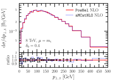
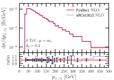
Figure 1: Comparison of predictions at NLO to those of MADGRAPH5/aMC@NLO [25] for transverse momentum of the top quark and the hardest photon. The lower panel shows the ratio of the predictions. For details on the selection cuts we refer to the text.

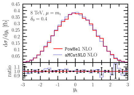
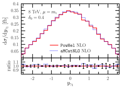
Figure 2: The same as Fig. 1 but for the top quark and hardest photon rapidities.

The cross section corresponding to our selection cuts both at LO and NLO can be found in Table 1. For illustrative purposes four sample distributions are shown on Figs. 1 and  2. As it can be seen from comparing the numbers obtained for cross sections at LO and NLO and from the distributions the two calculations are in agreement with each other.

4 Technical issues

4.1 Generation cuts

In a recent work [11] we proposed a new method to generate sufficiently inclusive LHEs including photons, which can be used to make predictions for the hadroproduction of isolated hard photons at the hadron level, formally correct at NLO accuracy in perturbative QCD. The essence of the method is to introduce generation isolation that is sufficiently loose so that the physical cross section with usual isolation parameters is independent of the parameters of the isolation needed for generating the events. For generation isolation we employ the smooth isolation of Frixione [22] with a small value for the parameter $\delta_{0}$. In addition to the isolation during event generation, we also need a generation cut on the transverse momentum of each photon, that we set to $5\,\,\mathrm{GeV}$ and varying it we checked that our physical predictions for hard photon production do not depend upon this cut.

4.2 Suppression factors

This process has two photons in the final state. As no photon-photon splitting is possible two technical cuts are sufficient to obtain a finite cross section at LO: lower limits are needed for the transverse momentum of the two photons. To enhance event generation in the physically relevant portion of phase space we use a suppression factor which could be used to suppress events in regions of phase space that are expected to be cut by physical selection cuts. Instead of this straightforward generalization of the suppression factor for the ${\rm t}\,\bar{{\rm t}}\,\gamma$ process [11] we suggest

$$\mathcal{F}_{\rm supp} =\frac{1}{1+\left(\frac{p_{\perp,{\rm supp}}^{2}}{p_{\perp,\,\gamma_{1}}^{2}}\right)^{k}+\left(\frac{p_{\perp,{\rm supp}}^{2}}{p_{\perp,\,\gamma_{2}}^{2}}\right)^{k}+\left(\frac{m_{\rm supp}^{2}}{m_{\gamma\gamma}^{2}}\right)^{k}}\,,$$ (2)

where $p_{\perp,\,\gamma_{i}}$ is the transverse momentum for the $i$th photon, $m_{\gamma\gamma}$ is the invariant mass of the two-photon system and $k=2$ was chosen throughout. The suppression over the invariant mass of the two-photon system is introduced to allow for a much better population of the large and moderately large $m_{\gamma\gamma}$ region. Our results were obtained with $p_{\perp,{\rm supp}}=100\,\,\mathrm{GeV}$ and $m_{\rm supp}=100\,\,\mathrm{GeV}$.

In the POWHEG-Box the differential cross section correct up to NLO has the form of

$$\mathrm{d}\sigma^{\rm NLO} =\mathrm{d}\Phi_{B}B+\mathrm{d}\Phi_{B}\mathcal{V}+\mathrm{d}\Phi_{B}\int\mathrm{d}\Phi_{\rm rad}(R-C)+\mathrm{d}\Phi_{B}\left(G_{\oplus}+G_{\ominus}\right)\,,$$ (3)

where $B$ is the Born term, $\mathcal{V}$ is the regularized virtual contribution, $R$ is the real-emission part, $C$ is a short-hand for all the local subtraction terms regularizing the real-emission, $G_{\oplus}$ and $G_{\ominus}$ are remnants of collinear factorization, $\mathrm{d}\Phi_{B}$ is the underlying Born while $\mathrm{d}\Phi_{\rm rad}$ is the one-particle phase space measure and the integral over momentum fractions is considered implicit. In the POWHEG-Box it is possible to decompose the real-emission part into two, disjoint contributions: the singular ($R^{s}$) and remnant ($R^{r}$) ones. Originally this bisection was introduced to deal with problems arising when the Born term becomes zero but not all the contributions [28]. This decomposition resulted in faster event generation and later on became standard [26]. With this decomposition the differential cross section takes the form of

$$\mathrm{d}\sigma^{\rm NLO} =\mathrm{d}\Phi_{B}B+\mathrm{d}\Phi_{B}\mathcal{V}+\mathrm{d}\Phi_{B}\int\mathrm{d}\Phi_{\rm rad}(R^{s}-C)+\mathrm{d}\Phi_{B}\left(G_{\oplus}+G_{\ominus}\right)+\mathrm{d}\Phi_{R}R^{r}=$$

$$=\mathrm{d}\Phi_{B}\widetilde{B}+\mathrm{d}\Phi_{R}R^{r}\,,$$ (4)

by introducing $\widetilde{B}$ we can now speak about a $\widetilde{B}$ and a remnant contribution. To decide whether a real-emission contribution is the singular or the remnant one, the following criterion is used as default in the POWHEG-Box:

$$R^{s}=R-R^{r}\,,\qquad R^{r}=R\,\Theta\left(R-\xi\max(C_{\mathcal{C}},C_{\mathcal{S}})\right)\,,$$ (5)

where $C_{\mathcal{C}}$ is the sum of all the collinear while $C_{\mathcal{S}}$ is the sum of all the soft subtraction terms and $\xi$ is an arbitrary parameter set to $5$ as default in the POWHEG-Box. When dealing with a process with photon(s) in the final state, hence having a generation isolation, large contributions can turn up when the separation between one of the photons in the final state and one final state massless quark becomes smaller than $\delta_{0}$. These contributions end up in the remnant provided by the large $R/B$ ratio degrading the efficiency of remnant-type event generation. This is a consequence of the method of event generation which is based upon the hit-and-miss technique: an overall upper bound is determined which is used in a subsequent step to unweight on the phase space. Large contributions tend to push this upper bound very high hence large difference can build up between the upper bound and regular contributions characterizing the vast majority of phase space hampering the unweighting procedure.

When the underlying Born process is already singular close to the singularity the contributions are enhanced due to the apparent, unregularized singularity. These large contributions result in a large norm which forces the hit-and-miss based event generation mechanism to generate almost all the events close to the singular region. This problem can be successfully solved by introducing a suppression factor which, as its name suggests, suppresses these large contributions by multiplying them with a dynamics-dependent, though small number. In the generated event file the phase space coverage of the events is such that less events are generated in and near singular regions. Since the suppression is a purely non-physical quantity the events can only bear physical meaning if the event weight incorporates the inverse of the suppression factor. Thus the suppression of the number of events in regions bearing no physical importance is compensated by scaling up the event weight accordingly.

The concept of the suppression factor can be used to improve the efficiency of remnant-type event generation. We modify the differential cross section by introducing a second suppression factor only affecting the remnant contribution:

$$\mathrm{d}\sigma^{\rm NLO} =\mathrm{d}\Phi_{B}\widetilde{B}+\mathrm{d}\Phi_{R}\mathcal{F}_{\rm supp}^{\rm r}(\Phi_{R})R^{r}\,,$$ (6)

where $\mathcal{F}_{\rm supp}^{r}(\Phi_{R})$ is the remnant suppression factor depending upon the real-emission phase space. To obtain physically meaningful events when a remnant event is being generated the event weight has to be multiplied by the inverse of the remnant suppression factor. Since large contributions to the remnant part of the cross section only come from those configurations where a final state (anti)quark is not well-separated from one of the photons the following form of remnant suppression was used during our calculations

$$\mathcal{F}_{\rm supp}^{r} =\prod_{i=1}^{2}\frac{1}{1+\left(\frac{p_{\perp,{\rm supp}}^{r}}{p_{\perp}(\gamma_{i},\,q)}\right)^{k}}\,,$$ (7)

where $p_{\perp,{\rm supp}}^{r}$ is the remnant suppression parameter set to $20\,\,\mathrm{GeV}$ throughout our calculation, $p_{\perp}(\gamma_{i},\,q)$ is the relative $p_{\perp}$ of the $i$th photon and the final state (anti)quark and we use $k=4$. The suppression is used only for those contributions where a massless (anti)quark is present in the final state. The presence and this form of remnant suppression significantly increased the efficiency of remnant event generation.

4.3 Choice of scale

The final state for ${\rm t}\,\bar{{\rm t}}\,\gamma\,\gamma$ production contains four particles at the Born level which leaves us with a rich set of kinematic variables usable for setting the renormalization and factorization scales for the process. In our previous work [13] for the hadroproduction of the t$\bar{{\rm t}}$ b$\bar{{\rm b}}$ final state, with massless b-quarks, we found that the half sum of the transverse masses of final state particles provides a good scale. It yields a moderate K-factor and small differences in the shapes of the distributions at LO and NLO accuracies. Thus we adopt the same choice for ${\rm t}\,\bar{{\rm t}}\,\gamma\,\gamma$ production for the central scale,

$$\mu_{0}=\hat{H}_{\bot}/2=\frac{1}{2}\left(m_{\bot,\,{\rm t}}+m_{\bot,\,\bar{{\rm t}}}+p_{\bot,\,\gamma_{1}}+p_{\bot,\,\gamma_{2}}\right)\,,$$ (8)

where the hat indicates that the underlying Born kinematics was used to construct the scale. We show the scale dependence of the cross section as the scale is varied around the central choice in Fig. 3. To make this prediction we used the following setup: 13 TeV LHC with CT10nlo as the chosen PDF set using a 2-loop $\alpha_{\rm s}$, $m_{\rm t}=172.5\,\,\mathrm{GeV}$ and the fine-structure constant kept fixed at $\alpha_{\rm EM}=1/137$. The selection cuts coincide with the set used in Sect. 3 with the inclusion of a cut on the separation of the two hard photons measured in the rapidity azimuthal angle plane, $\Delta R(\gamma_{1},\gamma_{2})>0.4$. The scales are varied by first making the renormalization and factorization scales coincide, $\mu_{\rm R}=\mu_{\rm F}=\mu$, then $\mu$ is varied through $\mu=\xi\mu_{0}$, where $\xi\in[1/16,8]$ and $\mu_{0}=\hat{H}_{\bot}/2$. Using this default scale, the NLO K-factor is $K\simeq 1.24$. If the scale is varied in the standard region of $[\mu_{0}/2,\,2\mu_{0}]$ the scale uncertainty drops from +30 %–27 % to +14 %–13 % if NLO QCD corrections are included. It is interesting to note that choosing $\mu_{0}=\hat{H}_{\bot}/4$ as default scale, the scale dependence remains the same, but the K-factor decreases to $K\simeq 1.08$.

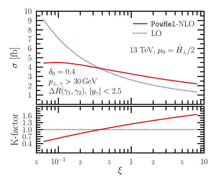
Figure 3: LO and NLO cross sections as functions of the scale variation parameter. Details of the setup and cuts applied can be found in the text.

4.4 The effect of the POWHEG Sudakov factor

When pre-showered events are generated, the POWHEG Sudakov factor may have an effect on measurable quantities through higher order terms in the perturbative expansion. Hence it is always informative to compare predictions at the NLO, that is at fixed order, and those predictions which are obtained from pre-showered events. In order to quantify the effect of the POWHEG Sudakov factor events were generated with the setup of Sect. 3 and the predictions drawn from these events were compared to those of the NLO calculation. Sample distributions can be found on Figs. 4–6. From these distributions, except for the transverse momentum of the extra parton, a good agreement can be seen between the fixed-order calculation and predictions drawn from pre-showered events. Taking a look at the prediction of the transverse momentum of the extra parton obtained using pre-showered events the usual Sudakov shape can be seen at smaller values while for large transverse momentum, $\log_{10}(p_{\perp}/\,\mathrm{GeV})>1.75$, the LHE prediction merges into the fixed order one. As we already pointed out in the case of ${\rm t}\,\bar{{\rm t}}\,\gamma$ production [11] the Sudakov shape gets distorted at around 0.75 and below due to the presence of the cut (Frixione isolation) acting on the real-emission part.

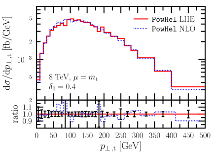
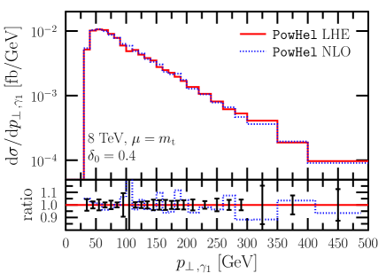
Figure 4: Comparison of the predictions at NLO accuracy to those obtained from pre-showered events for a configuration listed in the text for the transverse momentum of the top quark and for the hardest photon. The lower panel depicts the ratio of the two predictions.

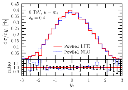
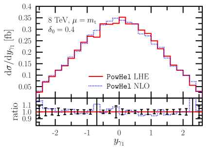
Figure 5: The same as Fig. 4 but for the rapidity of the top quark and the hardest photon.

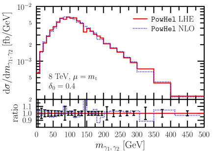
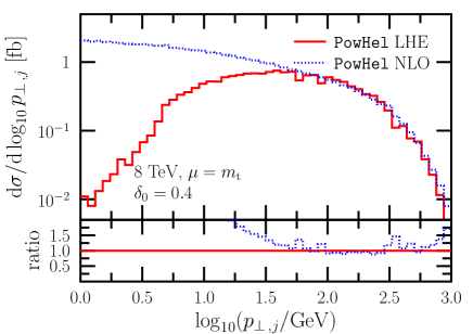
Figure 6: The same as Fig. 4 but for the invariant mass of the diphoton system and the transverse momentum of the extra parton.

5 Independence of the generation isolation

$\delta_{0}$	$\sigma^{\rm LHE}$ [fb]	$\sigma^{\rm PS}$ [fb]	$\sigma^{\rm SMC}$ [fb]
$0.01$	$3.31\pm 0.03$	$3.03\pm 0.04$	$2.17\pm 0.02$
$0.05$	$3.30\pm 0.03$	$3.07\pm 0.05$	$2.13\pm 0.02$
$0.1$	$3.33\pm 0.03$	$3.05\pm 0.03$	$2.18\pm 0.03$

Table 2: Cross sections obtained at different stages of event evolution for three different values of generation isolation using the cuts listed in the text.

In our previous work [11] we carried out an extensive study to prove the independence of generation isolation at various stages of evolution of the pre-showered events. For the present process we have repeated all steps, but we restrict ourselves to present the case of full SMC. At other stages of event evolution the predictions taken with different generation isolations are in agreement with each other. The events were generated for the setup listed in Sect. 4.3. For concreteness the cross sections obtained at various levels for different generation isolations are listed in Table 2. These cross sections correspond to the following set of cuts:

• Jets are reconstructed with the IR-safe anti-$k_{\perp}$ algorithm [29] with $R=0.4$ and $p_{\perp,j}>30\,\,\mathrm{GeV}$ using FastJet[30, 31].

• Two hard photons, $p_{\perp,\,\gamma}>30\,\,\mathrm{GeV}$, are requested in the central region, $|y_{\gamma}|<2.5$.

• The photons should be isolated from the jets and each other such that $\Delta R>0.4$. The separation is measured in the rapidity-azimuthal angle plane.

• The hadronic activity is limited around both photons in a cone of $R_{\gamma}=0.4$: $E_{\bot,\,{\rm had}}^{\rm max}=3\,\,\mathrm{GeV}$.

The hadronic activity in a cone of $R_{\gamma}$ around the photon momentum, $p_{\gamma}$, is measured through the total hadronic transverse energy deposited in this cone:

$$E_{\bot,\,{\rm had}}=\sum_{i\in{\rm tracks}}E_{\bot,\,i}\Theta\left(R_{\gamma}-R(p_{\gamma},p_{i})\right)<E_{\bot,\,{\rm had}}^{\rm max}\,,$$ (9)

where the summation runs over all the hadronic tracks. To make our predictions at the hadron level we used PYTHIA-6.4.25. At the hadron level we allowed tops to decay, but kept QED shower and multiparticle interactions inactivated. To see the independence of generation isolation we generated events with three different smooth isolation parameters ($\delta_{0}\in\{0.1,\,0.05,\,0.01\}$) and compared these pairwise. Sample distributions at the hadron level are depicted on Figs. 7–9. Among these distributions t-quark related observables can be found too. These were obtained by reconstructing the t-quark using MCTRUTH. From these distributions we can see that the deviation of predictions from each other is only due to statistical fluctuations. All of the event sets taken with the three different generation isolations result in the same predictions at the hadron level which means that any of these can be safely used in analyses to provide theoretical predictions.

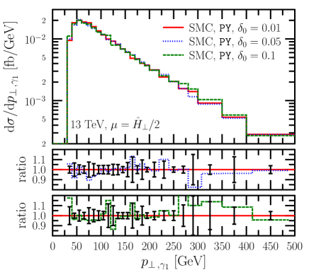
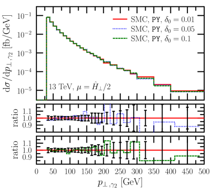
Figure 7: Comparison among predictions at the hadron level taken with three different generation isolation, $\delta_{0}=0.1$ (green dashed), 0.05 (blue dotted) and 0.01 (red solid), for the transverse momenta of the two hardest photons. The lower panels show the ratios with respect to the case of $\delta_{0}=0.01$.

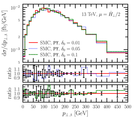
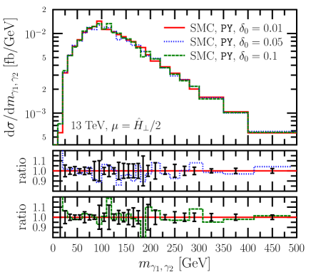
Figure 8: The same as Fig. 7 but for the transverse momentum of the top quark and the two-photon invariant mass.

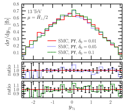
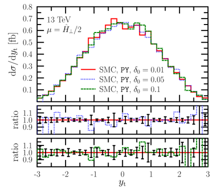
Figure 9: The same as Fig. 7 but for the rapidity of the hardest photon and the top quark.

6 Phenomenology

The main consequence of the previous two sections is the ability to make physical predictions with experimental isolation criteria using pre-showered events prepared with a generation isolation chosen suitably small. The ${\rm t}\,\bar{{\rm t}}\,\gamma\,\gamma$ production plays an important role in Higgs physics when attention is turned to the properties of the Higgs boson. One such important property is the Yukawa coupling of the Higgs boson to various massive fermions. The Yukawa coupling of the Higgs boson to the top quark can be measured in ${\rm t}\,\bar{{\rm t}}\,H$ production. When the Higgs boson decays in the diphoton channel the irreducible background is ${\rm t}\,\bar{{\rm t}}\,\gamma\,\gamma$ production. As we provided predictions for ${\rm t}\,\bar{{\rm t}}\,H$ production in Ref. [7] at the hadron level, we decided to present predictions for both the signal and the background at the hadron level with the highest available precision. For the ${\rm t}\,\bar{{\rm t}}\,\gamma\,\gamma$ background we take the events generated with $\delta_{0}=0.05$. For the signal we generated a new bunch of pre-showered events sharing the same parameters with the ${\rm t}\,\bar{{\rm t}}\,\gamma\,\gamma$ sample, generated for the 13 TeV LHC with CT10nlo PDF and accordingly chosen 2-loop $\alpha_{\rm s}$, $m_{\rm t}=172.5\,\,\mathrm{GeV}$, $m_{H}=125\,\,\mathrm{GeV}$. We chose the renormalization and factorization scales equal to each other and set to $\mu_{\rm R}=\mu_{\rm F}=m_{\rm t}+m_{H}/2$. To make our predictions, we used PYTHIA-6.4.25 for simulating the evolution of the events to the hadron level, but with multiple interactions turned off.

The partonic final state contains a t-quark pair for both the signal and the background. There are two ways to detect t-quarks: either through their decay products, by looking for displaced secondary vertices as tagging for decaying b-quarks, or using t-tagging. We decided to use the latter as provided by the HEPTopTagger [32, 33]. In order to perform t-tagging we followed the following steps:

• Jet reconstruction using all the hadronic tracks with the C/A algorithm with $R=1.5$ using FastJet[30, 31].

• Only those jets were considered for which $p_{\perp}>200\,\,\mathrm{GeV}$ and $|y|<5$.

• The t-quark candidate subjets were looked for in the jet mass range of 150 – 200 GeV.

• We selected that particular subjet as a t-quark jet for which the jet mass was the closest to $m_{\rm t}$.

In respect to other parameters concerning the top tagging we kept the default values provided by the HEPTopTagger. The cuts applied to the hadronic events were the following:

• Two hard photons were requested in the central region with $p_{\perp,\,\gamma}>30\,\,\mathrm{GeV}$ and $|y_{\gamma}|<2.5$.

• The photons should be isolated from each other: $\Delta R(\gamma_{1},\,\gamma_{2})>0.4$.

• To isolate the photons from hadronic activity a jet clustering was performed on all the hadronic tracks with the anti-$k_{\perp}$ algorithm [29] as implemented in FastJet[30, 31] with $R=0.4$ and $p_{\perp,j}>30\,\,\mathrm{GeV}$. The photons were requested to be isolated from these jets by $\Delta R(\gamma,j)>0.4$ measured on the rapidity-azimuthal angle plane.

• Both of the hard photons had to be isolated from the top jet obtained by top tagging and from the three subjets of the top jet by $\Delta R(\gamma,j)>0.4$ measured on the rapidity-azimuthal angle plane.

• One hard lepton was requested in the central region with $p_{\perp,\,\ell}>30\,\,\mathrm{GeV}$ and $|y_{\ell}|<2.5$. To select leptons we did not make any distinction between leptons and antileptons.

• The lepton had to be isolated from both the jets and the photons with $\Delta R(\ell,i)>0.4,\,i\in\{\gamma,j\}$ measured on the rapidity-azimuthal angle plane.

• Around both photons a minimal hadronic activity was allowed in a cone of $R=0.4$ such that $E_{\perp,\,{\rm had}}^{\rm max}=3\,\,\mathrm{GeV}$.

In order to reach reasonable statistics even for the signal we turned off all decay channels of the Higgs boson but the diphoton one and rescaled the event weights with the $H\to\gamma\,\gamma$ branching ratio. The most interesting distribution is the invariant mass of the two-photon system along with this a couple more distributions are depicted in Figs. 10 and  11. By taking a look at the distributions it is clear that the cross section drops into the attobarn range. Due to the narrow width of the Higgs boson the signal appears as a single, well-defined spike in the $m_{\gamma\gamma}$ spectrum with excellent signal/background ratio. For all the other distributions the background overwhelms the signal.

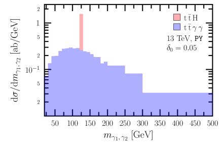
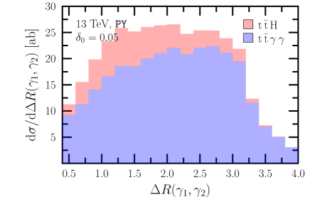
Figure 10: The invariant mass and rapidity azimuthal separation is shown for the diphoton system at the hadron level for the signal (${\rm t}\,\bar{{\rm t}}\,H$, red) and for the background (${\rm t}\,\bar{{\rm t}}\,\gamma\,\gamma$, blue) such that the signal sits on the top of the background. Further details of the calculation can be found in the main text.

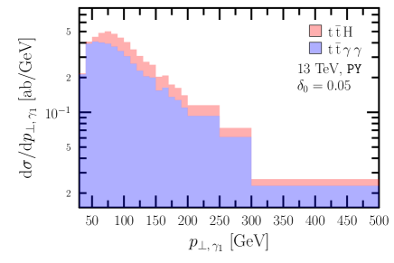
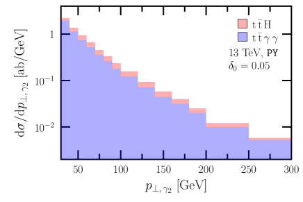
Figure 11: The same as Fig. 10 but for the transverse momentum of the two hard photons.

7 Conclusions

We presented the first predictions for the hadroproduction of ${\rm t}\,\bar{{\rm t}}\,\gamma\,\gamma$ final state both at NLO accuracy and at NLO matched with parton shower. The predictions at NLO were computed by two programs, PowHel and MADGRAPH5 and complete agreement was found. While the predicitions at NLO accuracy can be made only using smooth isolation prescription of Frixione for the hard photons, the matched predictions are based on LHEs that can be exposed to the usual cone-type isolation of experimenters. This is achieved by generating the events using generation cuts that are sufficiently loose, so that the predictions do not depend on those when usual physical isolations are used.

We found that using half of the sum of the transverse masses of particles in the final state the NLO corrections are about 25 %, and decrease the dependence on the renormalization and factorization scales significantly. The generated events are stored and can be downloaded from http://www.grid.kfki.hu/twiki/bin/view/DbTheory/TtaaProd. We generated similar events for the t$\bar{{\rm t}}$ $H$ final state, to which the ${\rm t}\,\bar{{\rm t}}\,\gamma\,\gamma$ process is an irreducible background in the $H\to\gamma\gamma$ decay channel. We compared some kinematic distributions of both signal and background process and found that the invariant mass of the two hard photons shows a clearly visible narrow peak, but with small cross section, in the attobarn range for the LHC at 13 TeV. For other kinematic distributions the signal and background have rather similar shapes.

Acknowledgements This research was supported by the Hungarian Scientific Research Fund grant K-101482, the SNF-SCOPES-JRP-2014 grant “Preparation for and exploitation of the CMS data taking at the next LHC run”, the European Union and the European Social Fund through LHCPhenoNet network PITN-GA-2010-264564, and the Supercomputer, the national virtual lab TAMOP-4.2.2.C-11/1/KONV-2012-0010 project.

References

- [1] ATLAS Collaboration Collaboration, G. Aad et. al., Observation of a new particle in the search for the Standard Model Higgs boson with the ATLAS detector at the LHC, Phys.Lett. B716 (2012) 1–29, [arXiv:1207.7214].
- [2] CMS Collaboration Collaboration, S. Chatrchyan et. al., Observation of a new boson at a mass of 125 GeV with the CMS experiment at the LHC, Phys.Lett. B716 (2012) 30–61, [arXiv:1207.7235].
- [3] ATLAS Collaboration Collaboration, G. Aad et. al., Evidence for the spin-0 nature of the Higgs boson using ATLAS data, Phys.Lett. B726 (2013) 120–144, [arXiv:1307.1432].
- [4] CMS Collaboration Collaboration, S. Chatrchyan et. al., Measurement of Higgs boson production and properties in the WW decay channel with leptonic final states, JHEP 1401 (2014) 096, [arXiv:1312.1129].
- [5] ATLAS Collaboration Collaboration, G. Aad et. al., Measurements of Higgs boson production and couplings in diboson final states with the ATLAS detector at the LHC, Phys.Lett. B726 (2013) 88–119, [arXiv:1307.1427].
- [6] CMS Collaboration Collaboration, S. Chatrchyan et. al., Measurement of the properties of a Higgs boson in the four-lepton final state, Phys.Rev. D89 (2014) 092007, [arXiv:1312.5353].
- [7] M. Garzelli, A. Kardos, C. Papadopoulos, and Z. Trócsányi, Standard Model Higgs boson production in association with a top anti-top pair at NLO with parton showering, Europhys.Lett. 96 (2011) 11001, [arXiv:1108.0387].
- [8] A. Kardos, Z. Trócsányi, and C. Papadopoulos, Top quark pair production in association with a Z-boson at NLO accuracy, Phys.Rev. D85 (2012) 054015, [arXiv:1111.0610].
- [9] M. Garzelli, A. Kardos, C. Papadopoulos, and Z. Trócsányi, Z0 - boson production in association with a top anti-top pair at NLO accuracy with parton shower effects, Phys.Rev. D85 (2012) 074022, [arXiv:1111.1444].
- [10] M. Garzelli, A. Kardos, C. Papadopoulos, and Z. Trócsányi, t and t Z Hadroproduction at NLO accuracy in QCD with Parton Shower and Hadronization effects, JHEP 1211 (2012) 056, [arXiv:1208.2665].
- [11] A. Kardos and Z. Trócsányi, Hadroproduction of t anti-t pair in association with an isolated photon at NLO accuracy matched with parton shower, arXiv:1406.2324.
- [12] A. Kardos, C. Papadopoulos, and Z. Trócsányi, Top quark pair production in association with a jet with NLO parton showering, Phys.Lett. B705 (2011) 76–81, [arXiv:1101.2672].
- [13] A. Kardos and Z. Trócsányi, Hadroproduction of t anti-t pair with a b anti-b pair using PowHel, J.Phys. G41 (2014) 075005, [arXiv:1303.6291].
- [14] S. Catani, M. Fontannaz, and E. Pilon, Factorization and soft gluon divergences in isolated photon cross-sections, Phys.Rev. D58 (1998) 094025, [hep-ph/9803475].
- [15] P. Nason, A New method for combining NLO QCD with shower Monte Carlo algorithms, JHEP 0411 (2004) 040, [hep-ph/0409146].
- [16] S. Frixione, P. Nason, and C. Oleari, Matching NLO QCD computations with Parton Shower simulations: the POWHEG method, JHEP 0711 (2007) 070, [arXiv:0709.2092].
- [17] S. Alioli, P. Nason, C. Oleari, and E. Re, A general framework for implementing NLO calculations in shower Monte Carlo programs: the POWHEG BOX, JHEP 1006 (2010) 043, [arXiv:1002.2581].
- [18] M. Garzelli, A. Kardos, and Z. Trócsányi, NLO Event Samples for the LHC, PoS EPS-HEP2011 (2011) 282, [arXiv:1111.1446].
- [19] G. Bevilacqua, M. Czakon, M. Garzelli, A. van Hameren, A. Kardos, et. al., HELAC-NLO, Comput.Phys.Commun. 184 (2013) 986–997, [arXiv:1110.1499].
- [20] J. Alwall, A. Ballestrero, P. Bartalini, S. Belov, E. Boos, et. al., A Standard format for Les Houches event files, Comput.Phys.Commun. 176 (2007) 300–304, [hep-ph/0609017].
- [21] S. Alioli, P. Nason, C. Oleari, and E. Re, Vector boson plus one jet production in POWHEG, JHEP 1101 (2011) 095, [arXiv:1009.5594].
- [22] S. Frixione, Isolated photons in perturbative QCD, Phys.Lett. B429 (1998) 369–374, [hep-ph/9801442].
- [23] Z. Kunszt, Z. Trócsányi, and W. J. Stirling, Clear signal of intermediate mass Higgs boson production at LHC and SSC, Phys.Lett. B271 (1991) 247–255.
- [24] A. Ballestrero and E. Maina, t anti-b H production for an intermediate mass Higgs, Phys.Lett. B299 (1993) 312–314.
- [25] J. Alwall, R. Frederix, S. Frixione, V. Hirschi, F. Maltoni, et. al., The automated computation of tree-level and next-to-leading order differential cross sections, and their matching to parton shower simulations, JHEP 1407 (2014) 079, [arXiv:1405.0301].
- [26] J. M. Campbell, R. K. Ellis, R. Frederix, P. Nason, C. Oleari, et. al., NLO Higgs Boson Production Plus One and Two Jets Using the POWHEG BOX, MadGraph4 and MCFM, JHEP 1207 (2012) 092, [arXiv:1202.5475].
- [27] A. Kardos, P. Nason, and C. Oleari, Three-jet production in POWHEG, JHEP 1404 (2014) 043, [arXiv:1402.4001].
- [28] S. Alioli, P. Nason, C. Oleari, and E. Re, NLO vector-boson production matched with shower in POWHEG, JHEP 0807 (2008) 060, [arXiv:0805.4802].
- [29] M. Cacciari, G. P. Salam, and G. Soyez, The Anti-k(t) jet clustering algorithm, JHEP 0804 (2008) 063, [arXiv:0802.1189].
- [30] M. Cacciari, G. P. Salam, and G. Soyez, FastJet User Manual, Eur.Phys.J. C72 (2012) 1896, [arXiv:1111.6097].
- [31] M. Cacciari and G. P. Salam, Dispelling the myth for the jet-finder, Phys.Lett. B641 (2006) 57–61, [hep-ph/0512210].
- [32] T. Plehn, M. Spannowsky, M. Takeuchi, and D. Zerwas, Stop Reconstruction with Tagged Tops, JHEP 1010 (2010) 078, [arXiv:1006.2833].
- [33] T. Plehn, M. Spannowsky, and M. Takeuchi, How to Improve Top Tagging, Phys.Rev. D85 (2012) 034029, [arXiv:1111.5034].