The low mass star and sub-stellar populations of the 25 Orionis group

Abstract

We present the results of a survey of the low mass star and brown dwarf population of the 25 Orionis group. Using optical photometry from the CIDA Deep Survey of Orion, near IR photometry from the Visible and Infrared Survey Telescope for Astronomy and low resolution spectroscopy obtained with Hectospec at the MMT, we selected 1246 photometric candidates to low mass stars and brown dwarfs with estimated masses within $0.02\raisebox{-2.15277pt}{$\,\stackrel{{\scriptstyle\textstyle<}}{{\sim}}\,$}M/M_{\odot}\raisebox{-2.15277pt}{$\,\stackrel{{\scriptstyle\textstyle<}}{{\sim}}\,$}0.8$ and spectroscopically confirmed a sample of 77 low mass stars as new members of the cluster with a mean age of $\sim$7 Myr. We have obtained a system initial mass function of the group that can be well described by either a Kroupa power-law function with indices $\alpha_{3}=-1.73\pm 0.31$ and $\alpha_{2}=0.68\pm 0.41$ in the mass ranges $0.03\leq M/M_{\odot}\leq 0.08$ and $0.08\leq M/M_{\odot}\leq 0.5$ respectively, or a Scalo log-normal function with coefficients $m_{c}=0.21^{+0.02}_{-0.02}$ and $\sigma=0.36\pm 0.03$ in the mass range $0.03\leq M/M_{\odot}\leq 0.8$. From the analysis of the spatial distribution of this numerous candidate sample, we have confirmed the East-West elongation of the 25 Orionis group observed in previous works, and rule out a possible southern extension of the group. We find that the spatial distributions of low mass stars and brown dwarfs in 25 Orionis are statistically indistinguishable. Finally, we found that the fraction of brown dwarfs showing IR excesses is higher than for low mass stars, supporting the scenario in which the evolution of circumstellar discs around the least massive objects could be more prolonged.

1 Introduction

Evidence collected over the past several years increasingly supports the general picture that low mass stars (LMS) and brown dwarfs (BDs), likely share a common formation mechanism. However, there are many open questions that remain to be addressed. For example, given typical temperatures and densities within molecular cloud cores (e.g. Padoan & Nordlund, 2004), the corresponding classical Jeans mass can be much higher than the sub-stellar mass limit ($\sim 0.072M_{\odot}$; Baraffe et al., 1998), suggesting that forming BDs would be difficult under such conditions. However, we know that not only do LMS and BDs form, but they do so abundantly, being the most numerous objects in the Galaxy (e.g. Padoan & Nordlund, 2004; Bastian, Covey & Meyer, 2010). Therefore, their formation cannot be explained in terms of a simple-minded model of gravitational collapse alone, which has been an important driver of theoretical and observational efforts looking for the physical processes and conditions that control LMS and BD formation.

Theoretical efforts to explain the formation of LMS and BDs are usually classified in the following models, reviewed by Whitworth et al. (2007): (i) turbulent fragmentation, (ii) gravitational fragmentation (iii) disc fragmentation (iv) premature ejection of protostellar embryos and (v) photo-erosion of cores in HII regions. These processes are not mutually exclusive (Whitworth et al., 2007) in the sense that in a typical star forming region (SFR) all of them could take place simultaneously, resulting in a complex scenario. The relative importance of each model is currently explored in terms of its ability to reproduce observables such as the initial mass function (IMF), the properties of binary and multiple systems, the fraction of LMS and BDs showing circumstellar discs, magnetosferic accretion and/or outflows and studying the kinematic or spatial segregation as a function of stellar mass (e.g. Whitworth et al., 2007). Each model has proven its plausibility of forming LMS and BDs, though only a few of the available simulations offer results directly comparable with observational data, and several assumptions about the initial conditions are still a matter of debate.

Observationally, several SFRs and young clusters have been surveyed looking for their LMS and BD population (e.g. Luhman, 2012; Luhman et al., 2010; Boudreault & Bailer-Jones, 2009; Bouvier et al., 2008; Lodieu et al., 2007; Caswell, 2007; Luhman et al., 2007, and references therein). Some important results are: the continuity of the mass function across the sub-stellar mass limit (e.g. Bastian, Covey & Meyer, 2010), the existence of circumstellar discs (e.g. Luhman et al., 2010), accretion phenomena (e.g. Muzerolle et al., 2000; Jayawardhana, Mohanty & Basri, 2003) and photometric variability (e.g. Scholz & Eislöffel, 2005) in BDs, which indicate the extension of the T-Tauri behaviour below the sub-stellar mass limit. There is also some initial insight on mass segregation (e.g. Kumar & Schmeja, 2007; Boudreault & Bailer-Jones, 2009), mass-dependent kinematics (e.g. Joergens, 2006) and multiplicity (e.g. McCarthy & Zuckerman, 2004; Luhman, 2004; Kraus, White & Hillenbrand, 2006; Luhman et al., 2009).

Here we present a new, deep optical/near infrared photometric survey of the 25 Orionis group, combined with limited follow-up spectroscopy, to search for and characterise the LMS ($0.8\raisebox{-2.15277pt}{$\,\stackrel{{\scriptstyle\textstyle<}}{{\sim}}\,$}M/M_{\odot}\raisebox{-2.15277pt}{$\,\stackrel{{\scriptstyle\textstyle<}}{{\sim}}\,$}0.072$) and BD ($0.072\raisebox{-2.15277pt}{$\,\stackrel{{\scriptstyle\textstyle<}}{{\sim}}\,$}M/M_{\odot}\raisebox{-2.15277pt}{$\,\stackrel{{\scriptstyle\textstyle<}}{{\sim}}\,$}0.02$) members of this population. The relevance of the 25 Orionis group for studies of star/disc formation and early evolution is given by its $\sim$7 Myr old age which roughly corresponds to the time when dissipation of primordial circumstellar discs is expected to have finished ($\sim$10 Myr; Calvet et al., 2005), as evidenced by the decrease in disc fractions (Hernández et al., 2006, 2007). Additionally, the study of the spatial distribution of members and/or the IMF down to the BD regime at this age, is important to constraint the dynamical evolution of young clusters (e.g. Boudreault & Bailer-Jones, 2009).

Other associations of similar age are either too spatially extended because of their vicinity (e.g. TW Hydra, $\beta$ Pictoris, $\epsilon$ Cha; Torres et al., 2008) or too distant (e.g. NGC7160, NGC2169, NGC2362 Kun, Kiss & Balog, 2008; Jeffries et al., 2007; Dahm, 2008). Lacerta OB1b at a distance of $\sim$400 pc and an estimated age within 12 to 16 Myr, is probably one of the best places to carry out new surveys for young LMS and BD, however, it also spans $\sim 70deg^{2}$ (Chen & Lee, 2008). Another interesting region, also spanning a large area of the sky, is the Upper Scorpius association at a distance between 125 and 165 pc (Luhman & Mamajek, 2012), whose last age determination is $\sim$11 Myr old (Pecaut, Mamajek & Bubar, 2012). Summarizing, the 25 Orionis group is the most numerous and spatially dense $\sim$7 Myr old population yet known within $\sim$500 pc from the Sun. Its modest angular extent ($\raisebox{-2.15277pt}{$\,\stackrel{{\scriptstyle\textstyle<}}{{\sim}}\,$}7deg^{2}$) makes comprehensive studies of its entire population feasible, and being almost free of significant interstellar extinction, it is the ideal place to study slightly more evolved young LMS and BD.

The paper is organized as follows: In Section 2 we summarize previous results on the 25 Orionis group. In Section 3 we describe the observations, data reduction, photometric candidate selection, as well as the spectroscopic confirmation of memberships for a sub-sample of these candidates. In Section 4 we estimate and analyse the visual interstellar extinction affecting each photometric candidate and spectroscopically confirmed member, and estimate the contamination from field stars present in the sample of photometric candidates. In Section 5 we present the derivation of masses and ages, the analysis of the IMF, the analysis of the spatial distribution and infrared excesses as disc indicators and accretion signatures. In Section 6 we summarize our conclusions about the nature of the 25 Orionis group and explore possible implications on predictions from theoretical models for LMS and BD formation.

2 The 25 Orionis group

The 25 Orionis group was originally identified by Briceño et al. (2005) as a $\sim 1^{\circ}$ radius overdensity of $\sim 20$ pre-main sequence (PMS) stars roughly centred on the Be star 25 Ori located at $\alpha_{J2000}=$05:24:44.8, $\delta_{J2000}=$+01:50:47.20. It was recognized on the basis of multi-epoch V and I-band photometry and follow-up optical spectroscopy to confirm memberships. Their initial member sample spanned magnitudes $14.5\raisebox{-2.15277pt}{$\,\stackrel{{\scriptstyle\textstyle<}}{{\sim}}\,$}V\raisebox{-2.15277pt}{$\,\stackrel{{\scriptstyle\textstyle<}}{{\sim}}\,$}16.5$, corresponding to masses in the range $0.45\raisebox{-2.15277pt}{$\,\stackrel{{\scriptstyle\textstyle<}}{{\sim}}\,$}M/M_{\odot}\raisebox{-2.15277pt}{$\,\stackrel{{\scriptstyle\textstyle<}}{{\sim}}\,$}0.95$. Briceño et al. (2005) reported a mean age for the Orion OB1a sub-association, which includes the 25 Orionis overdensity, of $\sim 7-10$ Myr and an inner-disc frequency of $\sim 11$ per cent, smaller than the $\sim 23$ per cent they had found in the younger ($\sim 3.6$ Myr) Orion OB1b sub-association. These results were consistent with the decrease in disc fraction with age seen in other regions (Hernández et al., 2008), and supported the idea that inner discs around low-mass stars dissipate in less than $\sim 10$ Myr (Hartmann, 2001).

The newly identified 25 Orionis group was also recognized a few months later by Kharchenko et al. (2005) in their extensive survey of new galactic clusters, and listed as cluster ASCC-16. They derive central coordinates $\alpha_{J2000}=$5:24:36, $\delta_{J2000}=$+01:48:00, a cluster radius=$0\aas@@fstack{\circ}62$ and core radius=$0\aas@@fstack{\circ}25$. They estimate a distance of 460 pc ($\rm V-M_{V}=8.59$), reddening $\rm E(B-V)=0.09$, age $\sim 8.5$ Myr, and a mean radial velocity of $0.75\pm 8.75$ km/s. However, the radial velocity comes from only one star, 25 Ori itself, and the age, distance and cluster radius are based on just a small number of stars earlier than K3.

The low-mass population of the 25 Orionis group was later considered by McGehee (2006). His variability-based survey of Orion OB1 using multi-epoch photometry from the Sloan Digital Sky Survey (Abazajian et al., 2005), within a $2\aas@@fstack{\circ}5$ wide equatorial strip located roughly $0\aas@@fstack{\circ}6$ south of the star 25 Ori. Based on the spatial distribution of his and Briceño et al. (2005) samples, McGehee (2006) suggested that the 25 Orionis group could extend further south, with a total radius of $\sim 1\aas@@fstack{\circ}4$, greater than previously reported. McGehee (2006) suggested that the 25 Orionis group is an unbound association and derived a Classical T-Tauri star (CTTS) fraction of $\sim 10$ per cent in what he called the 25 Orionis group.

Discs around the low-mass ($0.12\raisebox{-2.15277pt}{$\,\stackrel{{\scriptstyle\textstyle<}}{{\sim}}\,$}M/M_{\odot}\raisebox{-2.15277pt}{$\,\stackrel{{\scriptstyle\textstyle<}}{{\sim}}\,$}1.2$) members of 25 Orionis were searched for and characterised by Hernández et al. (2007) in their Spitzer IRAC and MIPS imaging study of this group. They found that in the 25 Orionis group, discs around low-mass stars are less frequent ($\sim 6$ per cent) than in the younger ($\sim 4$ Myr) Orion OB1b ($\sim 13$ per cent), and that this frequency seemed to be a function of the spectral type with a maximum around M0. They also determined that disc dissipation takes place faster in the inner region of the discs; as suggested by several disc models (e.g. Weidenschilling, 1997; Dullemond & Dominik, 2004).

After the initial discovery and first studies, Briceño et al. (2007) conducted the most extensive assessment so far of the low-mass population ($0.3\raisebox{-2.15277pt}{$\,\stackrel{{\scriptstyle\textstyle<}}{{\sim}}\,$}M/M_{\odot}\raisebox{-2.15277pt}{$\,\stackrel{{\scriptstyle\textstyle<}}{{\sim}}\,$}1$) in the 25 Orionis group. They concluded that not only is 25 Orionis a kinematically distinct entity, but it is also different in velocity space from the widely spread stellar population of Orion OB1a, within which it is located. These results pointed to the idea of the 25 Orionis group as a physical stellar group, akin to structures like the $\sigma$ Ori cluster. From the spatial distribution of the low-mass members they found a maximum surface density of $\sim 128$ stars/$deg^{2}$ with masses $M>0.5M_{\odot}$, and derived a cluster radius of $\sim$ 7 pc. In this work they also redetermined the fraction of Classical TTauri stars (CTTS) using a more numerous sample, and find disc fractions of $\sim 6$ per cent in 25 Orionis and $\sim 13$ per cent in Ori OB1b, confirming the factor of $2\times$ decline in the accretor fraction seen by Briceño et al. (2005).

The 25 Orionis group had been also the target for several other works: Using the Spitzer IRAC and MIPS data, Hernández et al. (2006) studied the debris disc fraction in stars with spectral types earlier than F5 in the 25 Orionis group. Biazzo et al. (2011) measured abundances for 8 T Tauri stars with spectral types from K7 to M0 and derived an average metallicity $[$Fe/H$]$=-0.05$\pm$0.05. Ingleby et al. (2011), have studied the X-ray and far ultraviolet fluxes of 25 Orionis and determined accretion rates for a set of members with spectral types K5 to M5. Most recently, 25 Orionis has been a hunting ground for groups looking for transiting planets among young solar-like stars (van Eyken et al., 2011; Neuhäuser et al., 2011). In Table 1 we summarize the derived parameters we assume here for the 25 Orionis group, based on the aforementioned studies and the present work. In Figure 1 we show the spatial distribution of candidates and confirmed members from previous surveys.

Table 1: General properties of members and candidates for the 25 Orionis group from the present and previous works.

Reference	Candidates	Members	Mass interval	LMS CTTS	LMS Discs	D	Radius	Age	$\bar{A_{V}}$
	[N]	[N]		[per cent]	[per cent]	[pc]	[∘]	[Myr]	[mag]
Briceño et al. (2005)	$\cdots$	31	$0.45\raisebox{-1.07639pt}{$\,\stackrel{{\scriptstyle\textstyle<}}{{\sim}}\,$}M/M_{\odot}\raisebox{-1.07639pt}{$\,\stackrel{{\scriptstyle\textstyle<}}{{\sim}}\,$}0.95$	$\sim 3$	$\sim 3$	330	$\cdots$	7-10	0.28
Kharchenko et al. (2005)	90	29	$M>1.4M_{\odot}$	$\cdots$	$\cdots$	460	0.62	$\sim 8.5$	0.27
McGehee (2006)	62	$\cdots$	$0.06\raisebox{-1.07639pt}{$\,\stackrel{{\scriptstyle\textstyle<}}{{\sim}}\,$}M/M_{\odot}\raisebox{-1.07639pt}{$\,\stackrel{{\scriptstyle\textstyle<}}{{\sim}}\,$}0.8$	$\sim 10$	$\cdots$	330	1.4	$\cdots$	$\cdots$
Hernández et al. (2007)	41	115	$0.12\raisebox{-1.07639pt}{$\,\stackrel{{\scriptstyle\textstyle<}}{{\sim}}\,$}M/M_{\odot}\raisebox{-1.07639pt}{$\,\stackrel{{\scriptstyle\textstyle<}}{{\sim}}\,$}1.2$	$\cdots$	$\sim 6$	330	$\cdots$	$\cdots$	$\cdots$
Briceño et al. (2007)	$\cdots$	124	$0.3\raisebox{-1.07639pt}{$\,\stackrel{{\scriptstyle\textstyle<}}{{\sim}}\,$}M/M_{\odot}\raisebox{-1.07639pt}{$\,\stackrel{{\scriptstyle\textstyle<}}{{\sim}}\,$}1$	$\sim 6$	$\cdots$	330	1	$\sim 7$	0.29
This work	1246	77	$0.02<M/M_{\odot}<0.8$	$3.8\pm 0.5$	$4.1\pm 0.4$	360	0.5	$6.1\pm 0.8$	0.30

3 Observations, candidate selection and membership determination

3.1 Optical photometry

Multi-epoch optical V, R, I-band, and H$\alpha$ observations across the entire Orion OB1 association (spanning $\rm\sim 180\>deg^{2}$) were obtained as part of the CVSO (Briceño et al., 2005), being conducted since 1998 with the Jürgen Stock 1.0/1.5 Schmidt-type telescope and the $8000\times 8000$ pixel QUEST-I CCD Mosaic camera (Baltay et al., 2002), at the National Astronomical Observatory of Venezuela. The instrument is composed of sixteen $2048\times 2048$ Loral CCD devices set in a $4\times 4$ array covering most of the focal plane of the telescope, and yielding a field of view $\sim 2\aas@@fstack{\circ}3$ wide in declination. The chips are front illuminated with a pixel size of $15\mu$m, which corresponds to a scale of 1.02” per pixel. Each row of four CCDs in the N-S direction can be fitted with a different filter. The system was optimized to operate in drift-scan mode, in which the telescope is fixed at a constant declination and hour angle, and an object moves across each filter as a consequence of sidereal motion, resulting in a survey rate of $\sim 34$ $deg^{2}$ per hour per filter. The scans for the CVSO were performed along strips centred at declinations $-5^{\circ}$, $-3^{\circ}$, $-1^{\circ}$, $+1^{\circ}$, $+3^{\circ}$ and $+5^{\circ}$ (for more details of the survey strategy see Briceño et al., 2005, 2007; Downes et al., 2008).

Because the exposure time in the drift-scan mode observations is fixed, this defines the usable magnitude range for each individual observation. At the bright end, our data saturate around magnitude 13 in the V, R and I bands, which corresponds to pre-main sequence (PMS) stars with masses $\sim 1M_{\odot}$, at the distance and age of the 25 Orionis group (Baraffe et al., 1998). At the faint end, the $3\sigma$ limiting magnitudes for individual scans are $\rm V_{lim}\sim 19.7$, $\rm R_{lim}\sim 19.7$, $\rm I_{lim}\sim 19.5$, with completeness magnitude of $\rm V_{com}\sim 18.7$, $\rm R_{com}\sim 18.7$, $\rm I_{com}\sim 18.2$. Again assuming Baraffe et al. (1998) models, and the age and distance of the 25 Orionis group ($\sim$7 Myr, $\sim$360 pc from Section 5.1), the substellar limit is located at $V_{sub}\sim 19.8$, $R_{sub}\sim 18.7$ and $I_{sub}\sim 17$, which clearly shows that individual scans are not sensitive enough for carrying out a complete study of the least massive BD in the Orion OB1 association.

In order to increase the signal to noise ratio (SNR) and therefore the limiting and completeness magnitudes, so that we could reach well into the substellar regime at the distance of Orion, we coadded the individual observations following the procedure explained in more detail in Downes et al. (2008). Summarizing, the process is based in the packages Offline and DQ developed by the QUEST-I collaboration (Baltay et al., 2002). In a first step, the QUEST-I data pipeline (Offline) automatically processes every single drift-scan considering each CCD of the mosaic as an independent device, corrects the raw images by bias, dark current and flat field, performs the detection of point sources, aperture photometry, and determines detector coordinates for each object. Then the software solves the world coordinate system by computing the astrometric matrices for each CCD of the mosaic, based on the USNOA-2.0 astrometric catalog (Monet, 1998).

After the basic processing for every individual scan has been done with the Offline package, the second step is to coadd these reduced single observations, using the package DQ. Using the transformation matrices output by Offline, the DQ package computes the offsets and rotations needed to place images of the same area of the sky, coming from different single drift-scans, in the same reference frame and add them pixel by pixel to produce the final coadded drift-scan. The coadded drift-scans used here are listed in Table 2, together with the mean coordinates, filter set, resulting limiting and completeness magnitudes for each photometric band after coadding, average FWHM of point sources, and number of individual scans included in the coadd.

Table 2: Observation log for the coadded drift-scans.

Drift-Scan	$\delta_{c}$	$\alpha_{ini}$	$\alpha_{end}$	Filters	FWHM	N	$V_{com}$	$R_{com}$	$I_{com}$	$V_{lim}$	$R_{lim}$	$I_{lim}$
	$J2000[^{\circ}]$	$J2000[^{\circ}]$	$J2000[^{\circ}]$		$[^{\prime\prime}]$
Single	+1, +3	65.00	99.00	All filters	2.5	1	18.7	19.0	18.5	20.5	20.5	20.0
Coadds 011-012	+1	76.14	86.30	VIIV	2.6	28	20.5	…	20.3	22.3	…	21.8
Coadd 013	+1	77.11	82.56	VIRI	2.8	29	20.5	20.8	20.3	22.3	22.3	21.8
Coadd 940	+1	67.00	98.22	RH$\alpha$IV	2.9	13	20.1	20.4	19.9	21.9	21.9	21.4
Coadd 950	+3	71.15	89.41	VRIV	2.6	10	19.9	20.2	19.7	21.7	21.7	21.2

In a third step, photometry and astrometry on the resulting coadded images are performed using an IRAF and IMWCS-based pipeline. The maximum number of detections at the $3\sigma$ threshold in the I-band images, corresponds to a mean spatial density of $\sim 1$ point source per $\sim 340$ arcsec square, resulting in a mean distance between nearest sources of about $\sim 22"$. Because of this, source crowding is not a problem, and we can safely perform aperture photometry; we used an aperture radius equal to the average FWHM of the coadded images ($\sim 3"$; Table 2).

The zero point calibration of the instrumental photometry in the Cousins system for each coadded drift-scan was done by normalizing the instrumental magnitudes to a master catalogue of $\sim 10^{5}$ non-variable stars with calibrated magnitudes. This large set of secondary standards was produced from a set of single drift-scans obtained with the same instrument and filters under photometric conditions, calibrated with Landolt (1992) standard star fields (Mateu et al., 2012). The calibration has an RMS of 0.021, 0.037 and 0.042 magnitudes in the $V$, $R$ and $I$ bands respectively. The mean positional uncertainty as inferred from the offsets in coordinates between the optical bands is 0.4″, with a standard deviation of 0.6″, similar to what we find for the offsets with respect to the infrared datasets we have used in this work (§3.2). Therefore, the photometric and astrometric calibration offer adequate accuracy for a reliable selection of LMS and BD candidates.

The catalogues with calibrated photometry for each photometric band from different coadded drift-scans, were finally compiled into a single deep catalog for each band, extracting repetitions and keeping, in such cases, always the measurement showing the highest SNR. We matched our optical source lists using a search radius of 3″, always keeping the object with the minimum positional difference. We will refer to this collection of four deep catalogs (in the V, R, I passbands and in a narrow band - 10 nm wide - H$\alpha$ filter), as the CIDA Deep Survey of Orion (CDSO, Downes et al. 2014 in preparation). The sources in the CDSO span the region $\rm 65^{\circ}\leq\alpha_{J2000}\leq 100^{\circ}$ and $-6^{\circ}\leq\delta_{J2000}\leq+6^{\circ}$, with positions and photometry for 8.6 million objects in the I-band, 8.1 million objects in the R-band, 6.9 million objects in the V-band, and 2.4 million objects in the H$\alpha$ filter.

In this contribution we focus on the LMS and BD populations of the 25 Orionis group, therefore we limit our analysis and discussion to drift-scans centred at declinations $+1^{\circ}$ and $+3^{\circ}$, in particular within the region $0\aas@@fstack{\circ}35\raisebox{-2.15277pt}{$\,\stackrel{{\scriptstyle\textstyle<}}{{\sim}}\,$}\delta\raisebox{-2.15277pt}{$\,\stackrel{{\scriptstyle\textstyle<}}{{\sim}}\,$}3\aas@@fstack{\circ}35$ and $79\aas@@fstack{\circ}7\raisebox{-2.15277pt}{$\,\stackrel{{\scriptstyle\textstyle<}}{{\sim}}\,$}\alpha\raisebox{-2.15277pt}{$\,\stackrel{{\scriptstyle\textstyle<}}{{\sim}}\,$}82\aas@@fstack{\circ}7$ shown in Figures 2, which encompasses the area expected to be spanned by the 25 Orionis group and its surroundings. In this area the I-band catalog has a limiting $\rm I_{lim}\sim 22$ and completeness $\rm I_{com}\sim 19.6$, which is enough to detect objects down to masses $\rm\sim 30\>M_{Jup}$, assuming Baraffe et al. (1998) models for the assumed age and distance of 25 Orionis. The full analysis of the entire CDSO will be presented in a forthcoming article.

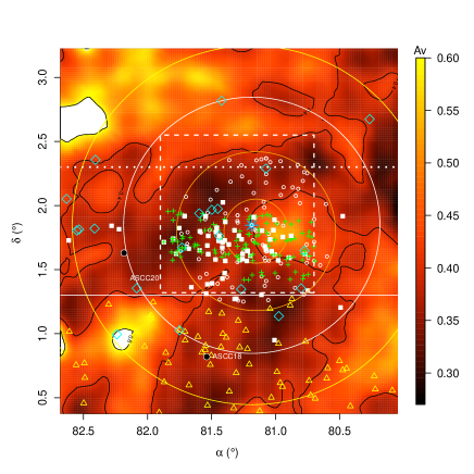
Figure 1: Spatial distribution of photometric candidates and confirmed members of the 25 Orionis group from previous studies. Solid squares: LMS confirmed as members from Briceño et al. (2005, 2007). The dotted horizontal line indicates the northern limit of the survey from Briceño et al. (2005). Small circles: Photometric and astrometric candidates from Kharchenko et al. (2005). Crosses: members and candidates from Hernández et al. (2006). Triangles: Photometric candidates from McGehee (2006). The solid horizontal line indicates the northern limit of the survey of McGehee (2006). Diamonds: Eclipsing systems and/or CTTS candidates from van Eyken et al. (2011). Large circles indicate from the centre outward: the core and corona cluster radii ($0\aas@@fstack{\circ}25$ and $0\aas@@fstack{\circ}62$ respectively) computed by Kharchenko et al. (2005), the radius suggested by Briceño et al. (2005) ($\sim 1^{\circ}$) and the radius proposed by McGehee (2006) ($\sim 1\aas@@fstack{\circ}4$); the dashed square indicates the spatial limits of the IRAC survey. Background: Map of the extinction A_V from Schlegel, Finkbeiner & Davis (1998) with scale on the right. The big central asterisk represents the 25 Ori star and the black dots other clusters from Kharchenko et al. (2005).

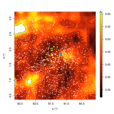
Figure 2: Spatial distribution of LMS and BD of the 25 Orionis group from the present work. Crosses: LMS and BD photometric candidates (§3.3). Circles: LMS confirmed as members (§3.5). The dashed circle indicates the field observed with Hectospec (§3.4). Other elements are as in Figure 1.

3.2 Infrared photometry

3.2.1 Near Infrared Data

As will be explained in Section 3.3, our technique of searching for young BDs and LMS in the extended off-cloud, low-extinction regions of the Orion OB1 association hinges on the combination of deep optical and near-infrared photometry. Ever since its release, the Two Micron All-Sky Survey (2MASS Skrutskie et al., 2006) has been the tool of choice for all large scale studies that required access to near infrared photometry for large numbers of sources over extended areas of the sky, with uniform spatial coverage. However, with limiting magnitudes of $\rm J_{lim}\sim 17.4$, $\rm H_{lim}\sim 16.7$, $\rm Ks_{lim}\sim 16.2$ and completeness magnitudes $\rm J_{com}\sim 16.6$, $\rm H_{com}\sim 15.8$, $\rm Ks_{com}\sim 15.4$, the 2MASS catalog is shallow compared to the deep CDSO data, imposing restrictions on our search for BD in Orion, in particular for the faintest, lowest mass objects. Nevertheless, being at the time of our initial candidate selection the only spatially complete near-IR dataset available, we cross matched our I-band CDSO catalog with 2MASS using a search radius of 3″, resulting in a master catalog with IJHKs photometry for each source. With this dataset we created the optical-near-IR colour-magnitude diagrams used to select LMS and BD candidates (see §3.3) for follow-up spectroscopy.

Recently, a new, much deeper near-IR survey has become available. During 2009 a new dedicated 4m survey telescope, the Visible and Infrared Survey Telescope for Astronomy (VISTA), located at ESO’s Paranal Observatory, was commissioned by the VISTA consortium (Emerson et al., 2004; Emerson & Sutherland, 2010). It is equipped with a 67$\times$10⁶ pixels camera with a scale of 0.34″/pix and a field of view of $1\aas@@fstack{\circ}65$ in diameter. For the Galactic Science Verification of VISTA, a $\rm\sim 30\>deg^{2}$ area of the Orion OB1 association, which included the Orion Belt region, part of the Orion A cloud, the 25 Orionis and $\sigma$ Ori clusters, was imaged in the Z, Y, J, H and Ks filters, during October 16 to November 2, 2009, down to $5\sigma$ limiting magnitudes $\rm Z\sim 22.5$, $\rm Y\sim 21.2$, $\rm J\sim 20.4$, $\rm H\sim 19.4$, $\rm Ks\sim 18.6$ (Petr-Gotzens et al., 2011). The data reduction was performed using a dedicated pipeline, developed within the VISTA Data Flow System, and run by the Cambridge Astronomy Survey Unit in the UK. The pipeline delivers science-ready stacked images and mosaics, as well as photometrically calibrated source catalogs. The final, band-merged Orion OB1 VISTA catalog contains $\sim$3 million sources. The VISTA photometric calibration is based on (but different from) 2MASS. Instrumental magnitudes were converted into apparent calibrated magnitudes on the VISTA system and calibrated via colour equations. This also included the Z and Y bands, following the procedure described in Hodgkin et al. (2009). The point sources detected in the I-band CDSO survey catalog were cross-matched with the VISTA Orion OB1 master catalog, using a 3″match radius. The resulting IZYJHKs catalog was then matched with our V, R and H$\alpha$ catalogs to add additional measurements in these bands for those objects which had them; however, the VRH$\alpha$ data were not used in the process of selecting LMS and BD candidates. Because VISTA goes much deeper than 2MASS, and since for objects in common the VISTA and 2MASS magnitudes agree within the uncertainties, we adopted the CDSO-VISTA dataset as our final optical-near IR photometry catalog. For objects showing $J<12$, $H<12$ or $Ks<11$ in the VISTA catalogue we adopted J, H and Ks magnitudes from 2MASS in order to avoid possible saturation effects in VISTA data.

3.2.2 Mid-infrared Data

In order to identify disc-bearing sources among selected candidate LMS and BDs, we matched our multiband VRH$\alpha$IZYJHKs catalog with our existing Spitzer observations within the 25 Orionis region obtained as part of GO-3437 (Hernández et al., 2007) and GO-50360 (Briceño et al. 2014, in preparation) and also with the recently released Wide Infrared Survey Explorer (WISE - Wright et al., 2010) database. First, a sub-sample of the photometric candidates and of the spectroscopically confirmed members (Sections 3.3 and 3.5), were identified in the object catalogs extracted from our IRAC images. The image reduction, point source detection and photometry for the datasets from Hernández et al. (2007) and Briceño et al. (2014, in preparation) are analogous and were described in Hernández et al. (2007). The IRAC observations were performed in the pass-bands centred at 3.6 $\mu$m, 4.5 $\mu$m, 5.8 $\mu$m and 8.0 $\mu$m with the spatial coverage shown in Figure 1. As a second step, the photometric candidates and spectroscopically confirmed members were identified in the WISE database which offers measurements in four pass-bands, centred at 3.4 $\mu$m, 4.6 $\mu$m, 12 $\mu$m and 22 $\mu$m. Compared to the IRAC observations, WISE is a shallow survey with worse angular resolution, but its spatial coverage is uniform, providing also data for the surroundings of 25 Orionis, where we did not have Spitzer data. The limiting and completeness magnitudes for each VISTA, IRAC and WISE photometric bands are summarized in Table 3 together with the number of photometric candidates and confirmed members from this work with available photometry from these IR surveys.

Table 3: Limiting and completeness magnitudes and the number of candidates and members from VISTA, IRAC and WISE surveys.

Survey	Band	Completeness	Limiting	Candidates	Members
VISTA	Z	22.5	23.5	1246	77
	Y	20.8	22.5	1246	77
	J	20.2	21.7	1246	77
	H	19.2	20.5	1246	77
	Ks	18.4	19.6	1246	77
IRAC	$3.6\mu m$	17.2	19.5	369	72
	$4.5\mu m$	16.7	19.0	388	77
	$5.8\mu m$	15.7	18.5	365	70
	$8.0\mu m$	14.7	17.5	358	77
WISE	$3.4\mu m$	16.2	17.2	1038	77
	$4.6\mu m$	16.0	17.0	1038	77
	$12\mu m$	12.8	13.2	1038	77
	$22\mu m$	9.1	9.5	1038	77

3.3 Selection of photometric candidates

The selection of photometric candidates was performed according to their position in colour-magnitude diagrams which combine optical and near infrared magnitudes. This method has been extensively used and has proved highly successful in identifying LMS and BDs in young clusters and star-forming regions (e.g Briceño et al., 2002; Luhman et al., 2003b; Downes et al., 2008).

We selected as candidates those objects located in what we call the membership locus, simultaneously in the I vs I-J, I vs I-H and I vs I-Ks colour-magnitude diagrams. These loci were defined as regions centred on the isochrone corresponding to the mean age from the Baraffe et al. (1998) models ($\sim$7 Myr) reported by Briceño et al. (2005, 2007) and a distance of $\sim$360 pc (Briceño et al. 2014, in preparation). The width of the loci were computed considering the 1 $\sigma$ uncertainties in age and distance, the mean interstellar extinction throughout the region, unresolved binarity, the 1 $\sigma$ photometric uncertainties and the expected mean intrinsic photometric variability. The resulting locus for the I vs. I-J diagram is shown in Figure 3. An object was considered as a photometric candidate if it was located within the membership locus in all three diagrams. Using the CDSO-VISTA catalog, a total of 1246 photometric candidates were selected inside the region showed in Figure 2, spanning a $\sim$ $2\aas@@fstack{\circ}5$ $\times$ $\sim$ $2\aas@@fstack{\circ}5$ area covering the previously known population of the 25 Orionis group and its surroundings.

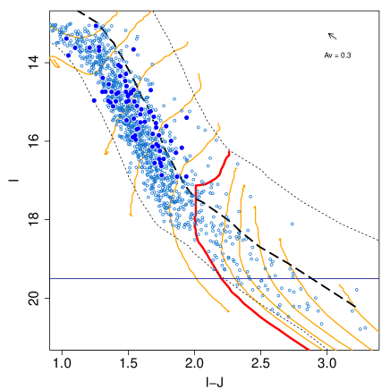
Figure 3: Color-magnitude diagram used as part of the candidate selection, including the objects selected as candidates (empty circles) and those confirmed as new members (big dots). The thick horizontal line indicates the completeness limit. The solid curves indicates evolutionary tracks for 0.8 M_⊙, 0.7 M_⊙, 0.5 M_⊙, 0.4 M_⊙, 0.1 M_⊙, 0.06 M_⊙, 0.05 M_⊙, 0.03 M_⊙, 0.02 M_⊙, 0.01 M_⊙ (thin) and 0.072 M_⊙ (thick). The thick dashed line indicates the isochrone corresponding to 7 Myr and the thin doted lines enclose the membership locus. Theoretical isochrones and evolutionary tracks are from Baraffe et al. (1998) models, are ploted without extinction correction and assuming $m-M=7.78$ magnitudes. The dereddening vector for the mean extinction throughout the region ($A_{V}=0.3$) is also indicated.

The estimated masses of the full candidate sample range from $\sim 0.8M_{\odot}$ down to $\sim 0.02M_{\odot}$ according to the models of Baraffe et al. (1998), with an age of $\sim$7 Myr and distance modulus of 7.78 mag. Due to the sensitivity and saturation of the I-band observations, the sample is complete from $\sim 0.8M_{\odot}$ ($I\sim 13$) down to $\sim 0.03M_{\odot}$ ($I\sim 19.6$). In Section 5.1 we present the estimation of ages and masses for each candidate.

We emphasize that colour-magnitude diagrams constructed combining optical and near infrared magnitudes yield the best selection of photometric PMS stellar candidates and young sub-stellar objects mainly because of two reasons: first, diagrams based on optical data alone (V, R and I-band magnitudes) suffer from an important completeness bias because BDs at this age and distance are red and very faint, so they drop out quickly in the bluer bands. Second, although our selection is not exempt from contamination by field stars, candidate selection performed in diagrams that include only near infrared data strongly increase the contamination by field dwarfs and by extragalactic sources, because of the limited leverage in colour; in these diagrams the isochrones are almost vertical and piled up, therefore, there is hardly any separation between the PMS locus and the field population. The contamination in our candidate sample by field stars and extragalactic sources is discussed in Section 4.2. The photometric variability in young LMS and BDs affects the optical and near-IR bands in a different way. Because our I-band data is the result from a coadd of images obtained in a period of 15 months, we considered that as the mean I-band magnitudes. The reported amplitudes of the variations in J, H and Ks-bands for LMS and BDs are within 0.2 to 0.5 mag (e.g. Scholz et al., 2009) We add to the width of the membership locus the corresponding change in colors that result from the maximum variation of 0.5 magnitudes in the near-IR bands.

3.4 Optical spectroscopy

Even with a refined selection technique, photometric candidate samples suffer from some degree of contamination by non-members like foreground field dwarfs and also by background giant stars and extragalactic objects. Therefore, spectroscopic follow up is necessary to unambiguously confirm membership. Moreover, spectra also provide crucial information necessary to derive fundamental properties, like the object’s effective temperature, $\rm A_{V}$, and hence its luminosity, whether it is accreting from a circumstellar disc, if it has a jet, and so on. Here we have extended in number and to much lower masses the member list discussed by Briceño et al. (2005, 2007), by obtaining low resolution (R$\sim$1000) optical spectra of a sample of 90 photometric candidates of the 25 Orionis group.

The spectra of the sample were obtained during the night of October 22 2007, during queue mode observations with the Hectospec multi-fiber spectrograph on the 6.5 MMT telescope (Fabricant et al., 2005). We observed a single field centred at $\alpha_{J2000}=$05:25:13, $\delta_{J2000}=$+01:39:25 (Figure 2), using one single fiber configuration for which we obtained five consecutive exposures, each 1800 s long. We used the 270 ${\rm groove\,mm^{-1}}$ grating, providing a spectral resolution of R$\sim$1000 with a spectral coverage from 3700 Å to 9150 Å. Because of the poor seeing conditions ($\sim 2.2^{\prime\prime}$) during the integrations and the diameter of the Hectospec fibers ($\sim 1.5^{\prime\prime}$), only the brightest candidates ($I\raisebox{-2.15277pt}{$\,\stackrel{{\scriptstyle\textstyle<}}{{\sim}}\,$}17$) could be observed with reasonable SNR ($\sim 15$), allowing for an appropriate spectral classification.

The 25 Orionis group is placed far enough from the Orion molecular clouds, so that problems due to the high sky background caused by nebulosity are not present. All the Hectospec spectra were processed, extracted, corrected for sky lines, and wavelength calibrated by S. Tokarz at the CfA Telescope Data Center, using customized IRAF routines and scripts developed by the Hectospec team (see Fabricant et al., 2005). The five individual 1800 s exposures were coadded into a single, deep observation, with a total integration time of 9000 s. Light sources inside the Hectospec fiber positioner, contaminate $\sim 1/3$ of the fibers at wavelengths longer than $\sim 8500$ Å (N. Caldwell, private communication), therefore, during the analysis we ignored data at these wavelengths.

Of the 1246 photometric candidates, 277 are placed within our Hectospec field. Because of limitations with the positioning of fibers and the poor seeing conditions we observed a total of 90 candidates out of which 77 were confirmed as new members of the 25 Orionis group for a $\sim$86 per cent efficiency. The remaining 13 candidates were confirmed as field stars. An example of the spectra is shown in Figure 4.

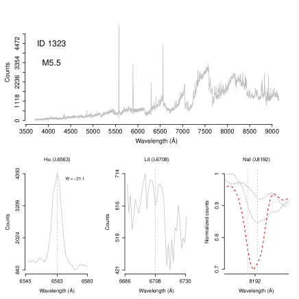
Figure 4: Spectra of a LMS confirmed in this work as a new member of the 25 Orionis group. The top panel shows the complete spectrum obtained by Hectospec and the lower panels the H$\alpha$ emission line, the LiI $\lambda 6708$ absorption line and the NaI $\lambda 8183,8195$ absorption doublet. Labels indicate the member ID, the spectral type and the equivalent width of H$\alpha$. Vertical dashed lines in the lower panels indicate the central wavelength of the H$\alpha$, LiI $\lambda 6708$ and NaI $\lambda 8183,8195$. In the panel for the NaI $\lambda 8183,8195$ absorption doublet we also show the corresponding spectra of a field dwarf (dashed red line; Kirkpatrick et al. (1999)), and a young dwarf from the Chamaeleon I region ($\sim$2 $Myr$; dotted line; Luhman et al. (2005)) of the same spectral type and smoothed to a same spectral resolution of 16 Å. The spectra for the entire sample of new members (see Table 4) are available in the electronic edition.

3.5 Spectral classification and membership diagnosis

We performed the spectral classification by comparing the equivalent widths of sixteen spectral features typical of M type stars, such as TiO and VO bands, (see Table 3 of Downes et al., 2008), with their corresponding values in a library of standard spectra of field dwarfs from Kirkpatrick et al. (1999), and following the semi-automated scheme of Hernández et al. (2004). The differences in surface gravity between the young targets and the field dwarfs used as standards did not affect significantly the spectral classification for objects earlier than M6. We estimate the typical uncertainty resulting from our classification to be $\pm$0.5 spectral subclass.

We have used several criteria to assign 25 Orionis group membership to each spectroscopically observed candidate. We start by considering the detection of H$\alpha$ in emission. Strong H$\alpha$ in emission is a common feature of chromospherically active young objects, and of objects accreting from a circumstellar disc for the largest equivalent widths (e.g. Muzerolle et al., 2005). Figure 4 shows the H$\alpha$ emission line profile and its corresponding equivalent width for a confirmed member. At the age of the 25 Orionis group ($\sim$7 Myr), most stars have stopped accreting (at least at significant levels), such that strong H$\alpha$ emission is not necessarily expected (Briceño et al., 2007), and many members could exhibit equivalent widths similar to those measured in active dMe stars. Therefore, as an additional membership indicator we looked at the NaI $\lambda 8183,8195$ absorption doublet. The NaI $\lambda 8183,8195$ feature is sensitive to the surface gravity of the star, being very strong (deep) in old field dwarf stars, very weak in late type M giants, and intermediate in late type PMS stars and young BDs which are still contracting down to the main sequence or asymptotically approaching the main sequence in the case of BDs (Luhman et al., 2003a). The NaI $\lambda 8183,8195$ absorption doublet of one of the LMS confirmed as member, superimposed on spectra of field dwarfs from Kirkpatrick et al. (1999), and of young M dwarfs of the same spectra type (from Luhman et al., 2003b) are shown in Figure 4. Given the typical I-J, I-H and I-Ks colours of the LMS and BD candidates considered here and the low visual extinction along the line of sight towards the 25 Orionis group, no reddened late giant stars are expected to contaminate our candidate sample, as we show in Section 4.2.

In addition to the above criteria, the presence of the Li I $\lambda 6708$ line in absorption was also considered. This spectral feature is a well-known indicator of youth in late K and M-type objects (Strom et al., 1989; Briceño et al., 1998, 2001), up to a spectral type $\sim$ M6.5, which at an age of $\sim$10 Myr corresponds to the mass limit for Li fusion ($M\sim 0.06M_{\odot}$ Basri, 1998). However, because of the low spectral resolution and SNR in most of our spectra, we could detect the LiI $\lambda 6708$ line in only $\sim 60$ per cent of the confirmed members. Objects showing Li I $\lambda 6708$ line in absorption were selected as members; those without a detection were not discarded as members unless they also failed the Na I criteria explained above.

Summarizing, photometric candidates were classified as members if they showed H$\alpha$ in emission and NaI $\lambda 8183,8195$ in absorption weaker than a field dwarf of the same spectral type. The detection of the Li I $\lambda 6708$ line in absorption was only considered as an additional youth indicator, in light of the bias imposed by the low spectral resolution and the SNR in most spectra. Additionally, as a sanity check, we looked at the $A_{V}$ of each star, computed from the observed colours and from the intrinsic colours we obtained from the spectral types and the relations from Luhman et al. (2003b), and noted whether it was consistent with the average $A_{V}$ for the 25 Orionis group (Briceño et al., 2007).

Clearly, the spectral features we have considered above are youth indicators but do not, by themselves, guarantee membership to the 25 Orionis group. The reason is that these same criteria will select young members that belong to other regions of the Orion OB1 association, placed behind the 25 Orionis group. Indeed, we know that 25 Orionis is located in the extended OB1a sub-association, and the much younger OB1b region is a few degrees away. However, as we argue in Section 4.2 the expected number of such possible young contaminants is low and does not affect the general analysis presented here. Additionally, the Hectospec field is centred in the 25 Orionis spatial overdensity we explain in Section 5.2, increasing the probability of these objects being real members of 25 Orionis group.

We confirmed 77 new members of the group whose photometric information and resulting spectral types are listed in Tables 4 and 5. In Figure 5 we show the H-R diagram with the new members.

Table 4: Photometric catalog of the new spectroscopically confirmed LMS of the 25 Orionis group. The table is published in its entirety in the electronic edition.

ID	$\alpha$ J2000	$\delta$ J2000	$V_{C}$	$R_{C}$	$I_{C}$	Z	Y	J	H	Ks	3.6$\mu$m	4.5$\mu$m	5.8$\mu$m	8.0$\mu$m
	[∘]	[∘]
1232	81.2582739	1.6224949	16.25	15.18	13.69	13.35	12.95	12.36	11.71	11.50	11.45	11.24	11.38	11.18
1242	81.0372844	1.7311253	16.11	15.09	13.66	13.18	12.68	12.07	11.57	11.39	11.17	11.11	11.07	11.10
1245	81.0632586	1.9016645	20.61	19.24	16.90	16.32	15.56	14.98	14.51	14.16	13.77	13.72	13.67	13.65
1246	81.2778866	1.7987624	19.16	17.83	15.65	15.12	14.46	13.89	13.40	13.11	12.69	12.64	12.57	12.54
1247	81.0647164	1.9310005	17.22	16.03	14.28	13.85	13.28	12.75	12.25	11.96
1248	81.2432939	1.9759851	17.45	16.38	14.73	14.33	13.86	13.36	12.77	12.56		12.22		12.17
1252	81.270781	1.6148316	16.92	15.81	14.1	13.64	13.17	12.61	12.04	11.81	11.49	11.49	11.48	11.47
1253	81.1664269	1.3613049	15.29	14.36	13.38	12.96	12.63	12.30	11.60	11.42	11.29		11.25
1258	81.2160937	1.541317		18.58	16.29	15.72	14.98	14.38	13.91	13.56	13.17	13.10	13.11	13.14
1261	81.0869439	1.4013985	15.69	14.74	13.62	13.32	13.00	12.47	11.77	11.65	11.47		11.40

Table 5: Spectroscopic catalog of the new confirmed members of the 25 Orionis group. The table is published in its entirety in the electronic edition.

ID	ST	W[H$\alpha$]	LiI	Av
		[$\AA$]		[mag]
1278	M4.5	-5.8	0	0
1273	M5	-13	1	0.12
1262	M4.5	-8.4	1	0
1277	M3.5	-4.3	-1	0
1284	M4.5	-9.9	1	0
1269	M4.5	-16.7	1	0.46
1263	M2.5	-5	1	0.54
1266	M4	-8.9	1	0.06
1279	M3.5	-8.9	0	0.21
1242	M3.5	-6.6	1	0.79

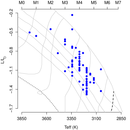
Figure 5: H-R diagram for the new members. The isochrones for 1, 3.2, 4.6, 8.5, 11.4 and 100 (dotted) Myr and the evolutionary tracks for 0.8 M_⊙, 0.6 M_⊙, 0.5 M_⊙, 0.3 M_⊙, 0.2 M_⊙, 0.1 M_⊙ and 0.072 M_⊙ (dashed) from the Baraffe et al. (1998) models are indicated. The top axis indicates the corresponding spectral types from Luhman et al. (2003b).

4 Interstellar extinction and contamination by field stars

One of the problems encountered when carrying out photometric surveys over large areas of the sky is obtaining follow-up spectroscopy for every single source of interest, thereby making sure one has positively identified every member of the stellar population of interest. Even with the multiplexing capabilities of modern day multi-fiber spectrographs, this can be a daunting task, specially if one needs to use very long exposure times in order to get enough SNR on very faint objects. However, in our case, we can extend our study of the 25 Orionis group beyond the spatial and mass completeness of the spectroscopically confirmed member sample, by a judicious use of the photometric candidate member sample. At the expense of a larger degree of contamination from non-members, the photometric sample has the virtue of providing a spatially complete rendering of the 25 Orionis aggregate, and it also allows us to sample large numbers of objects down to much lower masses. The disadvantage of this approach is that issues like contamination from non-members and variable extinction could potentially render any reliable analysis as useless. However, we will show that in the particular case of the 25 Orionis group, conditions are such that a photometric study of the group properties is not only feasible, but quite reliable.

4.1 Interstellar extinction

We determined the visual extinction $A_{V}$ for each of the 77 spectroscopically confirmed members, calculated by using the intrinsic I-J colour for the corresponding spectral type proposed by Luhman et al. (2003b), the observed I-J colour, and the Cardelli, Clayton & Mathis (1989) extinction law assuming R${}_{V}=$ 3.09. The resulting $A_{V}$ values are in excellent agreement with previous spectroscopic determinations by Briceño et al. (2005) for stellar members, as we show in Figure 6.

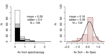
Figure 6: Distribution of the visual extinction $A_{V}$ throughout the 25 Orionis group. Left panel: $A_{V}$ values measured from spectra as explained in the text, from Briceño et al. (2005, 2007) (black), from this work (gray), and the complete sample (white). Right panel: Distribution of the residuals between visual extinctions computed from spectroscopy, and those from the Schlegel, Finkbeiner & Davis (1998) maps, for the same complete sample of the left panel. Solid line indicates the normal distribution which fits the data, with $\bar{A_{V}}=0.16$ and $\sigma=0.39$ magnitudes after removing the outliers.

The $A_{V}$ for the 1246 photometric candidates were derived using the Schlegel extinction maps (SEM; Schlegel, Finkbeiner & Davis, 1998). This approach is valid in this particular region because it has a spatially smooth extinction. Still, estimates from SEM have two main limitations: First, the $A_{V}$ reported in the SEM is the integrated extinction along the line of sight, limited by the sensitivity of the survey and the resulting $A_{V}$ for a nearby object will be overestimated, due to extinction sources behind the object. Second, the low spatial resolution of the SEM could result in an inadequate interpolation for objects placed in regions with abrupt variations of the extinction.

In order to assess how much we would overestimate the extinction by using the SEM, we computed a mean excess in $A_{V}$ by comparing the distribution of the residuals between $A_{V}$ computed using spectroscopy for the members confirmed in this work and those from Briceño et al. (2005), and $A_{V}$ from the SEM as we show in Figure 6. Except for a few outliers, the resulting distribution is essentially normal, with a mean $\bar{A_{V}}=0.16$ and standard deviation $\sigma_{A_{V}}=0.39$. We consider this average $\bar{A_{V}}$ as the mean excess extinction added by the SEM. Regarding the issue of limited spatial resolution of the SEM, from Figure 1 it is clear that the background towards the 25 Orionis group is quite smooth, showing no significant spatial variations ($\sigma_{A_{V}}\sim 0.2$). This uniformity is also confirmed in our Spitzer-MIPS 24$\mu$m images of this area (Hernández et al., 2007) and by preliminary extinction maps performed on the basis of near IR photometry from VISTA (Alves, private communication).

Thus, we estimated the $A_{V}$ for each photometric candidate by interpolating in the SEM and subtracting the $\bar{A_{V}}$ estimated from the distribution of residuals. We consider the mean uncertainty of our estimation over the entire sample of candidates as $\sigma_{A_{V}}/\sqrt{N}=0.03$ magnitudes, where $N=134$ is the number of confirmed members used for the residual distribution.

4.2 Contamination of the photometric candidate sample by field stars and extragalactic sources

There are three main possible sources of contamination of a LMS and BD photometric candidate sample from a star forming region: field dwarf and giant stars, unresolved extragalactic sources and, in our case, young stars belonging to other sub-regions such as Orion OB1a. Such contamination could affect estimates of the IMF, the mean age and the spatial distribution of the 25 Orionis group when performed using only photometric candidates. We use a Galactic model to estimate the contamination by Orion non-members towards our field, and since we obtained a large number of spectra, we can verify the predictions from such models.

The number of field stars, of all kinds, in the photometric candidate sample, was estimated from a simulation of the expected galactic stellar population in an area of $\sim 6.4deg^{2}$ centred at the 25 Orionis group, performed with the Besançon Galactic model (Robin et al., 2003). This model has been extensively tested and correctly reproduces the luminosity function within the sensitivity limits of the 2MASS survey (Robin et al., 2003). Second, we reproduce in the Besançon data the typical photometric incompleteness from our survey according to the following procedure: First, we ran the model simulation in the range 13$<$I$<$22 and simulating the photometric errors as function of magnitude, using an exponential function with parameters obtained from fitting our survey data. Second, to estimate the fractional contamination in our photometric survey we need to remove objects from the Besançon model in order to reproduce the fall-off as a function of magnitude observed in our survey. To do this we produced I vs. I-J Hess diagrams for our survey and the simulated sample using 0.1$\times$0.1 magnitude bins and randomly discarded simulated objects in each bin until their number matched our observed number. After this correction was applied, a star from the Besançon simulation was considered a contaminant of the photometric candidate sample if it satisfied the selection criteria explained in Section 3.3.

The resulting sample of contaminants is constituted exclusively by 212 low-mass main sequence stars that have an homogeneous spatial distribution with a mean spatial density of $\sim$33 objects per $deg^{2}$, estimated spectral types from K7 to L0 and distances between $\sim$50 pc and $\sim$300 pc. In our spectroscopic sample, every single star rejected as a member turned out to be a field dwarf, several with some degree of emission in H$\alpha$ as seen in dMe stars, but all showing the deep Na I 8183,8195 absorption expected in older, low-mass disc stars. No late type giants were found among the rejected, non-member, spectroscopic sample as suggested by our results from Besançon. In order to estimate the contamination as a function of member’s mass, we assume such contaminant field dwarf stars mistaken for members of the 25 Orionis group, and we computed the masses and ages they would have, following the procedure we will explain in Section 5.1, resulting in the distributions we show in Figures 7 and 8.

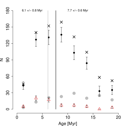
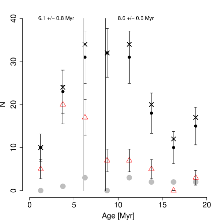
Figure 7: Distribution of ages for the full sample of stellar and sub-stellar candidates and confirmed members in the complete area of the survey (left) and inside a circle with radius 0.5^∘ centred at the 25 Orionis group overdensity defined in Section 5.2 (right). The distribution corresponding to photometric candidates (crosses) was corrected by subtracting the expected contamination by field stars (gray circles), resulting in the distribution indicated with black dots and the corresponding error bars. The triangles indicate the distribution for the spectroscopically confirmed members from this work and from Briceño et al. (2005). The distribution for members is the same in both plots because the spectroscopic sample covers only the overdensity. Top labels and vertical lines indicate the mode and standard deviation of the distributions from confirmed members (left) and from photometric candidates (right).

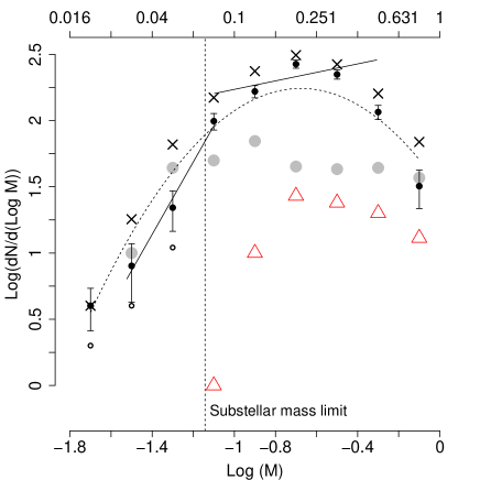
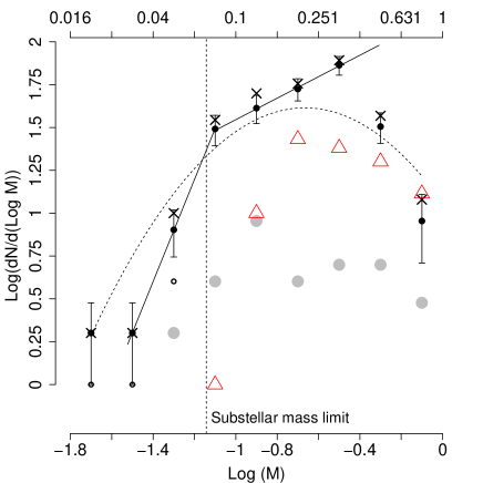
Figure 8: The system-IMF for the two samples considered in the Figure 7. The system-IMF from photometric candidates (crosses) was corrected by subtracting the expected contamination by field stars (gray circles), resulting in the system-IMF indicated with black dots and error bars. The empty circles indicate the system-IMF before the completeness correction was applied for objects with masses $M<0.06M_{\odot}$. The triangles indicate the system-IMF for the spectroscopically confirmed members, which is still largely incomplete. We compute all the distributions using bins of 0.2 dex. The dotted and solid curves indicate the best-fit to a log-normal distribution and a Kroupa power-law function.

We compared the observational J vs J-Ks diagram with those obtained from an appropiate simulation with the Besançon Galactic model (Robin et al., 2003) of the expected galactic population in the area covered by the survey (see Section 4.2). We found that the point sources showing J-Ks¿1.5 are spatially unresolved extragalactic objects that are not predicted by the Besançon galactic model. Then, we applyed to the selected extragalactic sources our criteria for the selection of photometric candidates to members of the 25 Ori group and found that only a negligible number of unresolved extragalactic sources ($\sim$1 source per $deg^{2}$) do satisfy our criteria for photometric candidate selection; this means a total of $\sim$7 extragalactic sources is expected in the entire sample of photometric candidates.

Summarizing, we found 1246 member candidates in the 25 Orionis group in the mass range considered here. If we neglect the contamination due to extragalactic sources and members from other regions of Orion OB1, from the Besançon model we expect 316 field dwarfs within the sample for a mean density of $\sim$33 contaminants per $deg^{2}$. The total number of candidates expected to be real members of the 25 Orionis group in the mass range considered here is 930 corresponding to a mean spatial density of $\sim$146 members per $deg^{2}$. Thus, our photometric selection has a global efficiency of $\sim$82 per cent which is in good agreement with the 77 new confirmed members which corresponds to the $\sim$86 per cent of our spectroscopic survey because spectra were obtained in the overdensity of candidates explaines in Section 5.2. We emphasize that the contamination shows a dependence with photometric colour which results in the fiducial mass and age distributions shown in Figures 7 and 8, which would be the mass and age distributions resulting from wrongly considering such contaminants as members.

5 Analysis and results

5.1 The mean age and the initial mass function

The masses and ages we derived here for the 25 Orionis low-mass population were obtained through interpolation of the luminosity and effective temperatures in the Baraffe et al. (1998) models, adopting a distance of 360 pc from Briceño et al. (2014, in preparation). For the photometric candidates we interpolated the luminosity and the effective temperature we obtained by interpolation of the I-band magnitude and the I-J photometric colour, both corrected by interstellar extinction as explained in Section 4.1, using the relationships from Luhman et al. (2003b) and Dahn et al. (2002), from which we obtained the effective temperatures and bolometric corrections. For the spectroscopically confirmed members we followed two procedures: First, as we did for the photometric candidates. Second, by interpolation of the measured spectral types in the same relationships. Within the uncertainties, no significant differences were found for masses and ages derived with either procedure for the spectroscopically confirmed member sample. This similarity is not surprising, given the low and smooth interstellar reddening towards this region, and the $\sim$0.5 spectral subclass mean uncertainty in the estimation of spectral types.

We derived the distribution of ages and the system-IMF for the photometric candidates and for the confirmed members in the entire area of our survey and in the spatial overdensity that will be defined in Section 5.2 as the 25 Orionis group overdensity. Figure 7 shows the resulting distribution of ages for photometric candidates and for spectroscopically confirmed members including also the members from Briceño et al. (2005) within the same mass interval. The member sample is still largely incomplete and biased toward the brighter (more massive) objects, but as can be seen in Figure 7, this bias does not strongly affect the estimation of age. The distribution corresponding to photometric candidates was corrected by subtracting the age distribution for the expected contamination by field stars, i.e. the age distribution that results from mistaking the contaminants as members of the 25 Orionis group.

We found a good agreement between the distributions of ages computed from photometric candidates and from spectroscopically confirmed members. In the complete area of the survey, the derived age of the 25 Orionis group is $7.7\pm 0.6$ Myr from candidates and $6.1\pm 0.8$ Myr from confirmed members. In the spatial overdensity, where the new members were detected, we found a mean age of $8.6\pm 0.6$ Myr from candidates. All the ages reported correspond to the mode of each distribution. We adopt the age derived from the confirmed members ($6.1\pm 0.8$ Myr) as the age of the 25 Orionis group, although this value is statistically indistinguishable from that obtained from photometric candidates. Therefore we confirm the age derived in previous works by our group ($\sim$7 Myr ; Briceño et al., 2007). In this new sample we are including several new spectroscopically confirmed members and photometric candidates covering a much wider magnitude range which allows for a more robust estimation of the mean age. Additionally, our result shows that the population within the 25 Orionis group is not distinguishable from the surrounding population in terms of their ages alone.

Figure 8 shows the system-IMF in the LMS and BD regime for the photometric candidates of the 25 Orionis group. Although the photometric completeness of our survey (I=19.6) is equivalent to a completeness mass limit of 0.03 $M_{\odot}$ assuming the Baraffe et al. (1998) models with an age of 7 Myr old and a distance modulus of m-M=7.78, the width of the membership loci defined in Section 3.3 and the dispersion of the candidates within it, suggest that some objects more massive than 0.03 $M_{\odot}$ could be located below the photometric completeness. In order to account for such incompleteness in our sample we estimated, per magnitude bin, the number fraction of missing objects as the ratio between the expected and observed number of objects fainter than the completeness magnitude. Figure 8 shows the system-IMF obtained after this completeness correction and the correction for the contamination by field stars were applied.

Because we did not apply any correction to account for unresolved binaries, what we report is the so called system-IMF of the 25 Orionis group (see e.g. Parravano, McKee & Hollenbach, 2010, and references therein). Although the system-IMF does not reveal by itself the real number of objects per mass bin, it is useful for comparison with system-IMFs from other SFR and young clusters, assuming that the samples have similar spatial resolution, and that the populations have similar multiplicity properties such as the number fraction of objects belonging to multiple systems, separation and mass ratio distributions.

We describe the derived system-IMF according to a Kroupa power-law function $\Psi(m)=dN/dm\propto m^{-\alpha_{i}}$ (Kroupa, 2001, 2002), and a Scalo log-normal function (Scalo, 1986) in the form $\Psi(\log m)=dN/d(\log m)\propto exp{-((\log m-\log m_{c})^{2}/2\sigma^{2})}$ (Chabrier et al., 2005). We fitted the mass distributions within the mass range $0.03<M/M_{\odot}<0.8$ to the log-normal function and within the mass ranges $0.03<M/M_{\odot}<0.08$ and $0.08<M/M_{\odot}<0.5$ for the power-law description. As we did for the age estimate, we obtain the system-IMF for the candidates inside the spatial overdensity (see Section 5.2) and for the entire area of the survey. For the latter, the system-IMF for masses in the intervals $0.03<M/M_{\odot}<0.08$ and $0.08<M/M_{\odot}<0.5$ follows Kroupa-type functions with $\alpha_{3}=-1.73\pm 0.31$ and $\alpha_{2}=0.68\pm 0.41$ respectively, and that in the complete mass interval $0.03<M/M_{\odot}<0.8$ is well described by a log-normal function with coefficients $m_{c}=0.21^{+0.02}_{-0.02}$ and $\sigma=0.36\pm 0.02$. For the spatial overdensity we found $\alpha_{3}=-1.97\pm 0.02$, $\alpha_{2}=0.37\pm 0.04$, $m_{c}=0.22^{+0.02}_{-0.02}$ and $\sigma=0.42\pm 0.05$. In Figure 8 and Table 6 we show the resulting fits and in Figure 9 we compare our derived IMF with other IMFs from the literature in which no correction for binarity was made.

Table 6: Fit parameters for the system-IMF.

Population	M interval	$\alpha_{2}$	$\alpha_{3}$	$m_{c}$	$\sigma$	Reference
25 Orionis overdensity	$0.03<M/M_{\odot}<0.8$	$0.37\pm 0.04$	$-1.97\pm 0.02$	$0.22^{+0.02}_{-0.02}$	$0.42\pm 0.05$	This work
25 Orionis entire area	$0.03<M/M_{\odot}<0.8$	$0.68\pm 0.41$	$-1.73\pm 0.31$	$0.21^{+0.02}_{-0.02}$	$0.36\pm 0.02$	This work
Field	$M<M_{\odot}$	…	…	$0.22$	$0.57$	Chabrier (2003b)

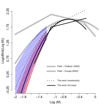
Figure 9: Comparison of the system-IMF obtained for the 25 Orionis group with those from Chabrier (2003b) and Kroupa (2001, 2002). The black solid curve and straight lines correspond to the fit to a log-normal and power-law functions for the entire area of the survey respectively. The gridded area indicates, in the BD regime, the uncertainty in the fit to the log-normal function. The dotted curve and straight lines: fit to a log-normal and power-law functions for the spatial overdensity. The dashed area indicates, in the BD regime, the uncertainty in the fit to the log-normal function. Gray curve: IMF from Chabrier (2003b). Gray solid lines: IMF from Kroupa (2001, 2002).

Additionally, we computed the distribution of spectral types, which is generally used as a proxy of the IMF which avoids most of the uncertainties related to the computation of masses (e.g. Preibisch, 2012). Figure 10 shows the spectral type distributions for confirmed members and photometric candidates. For the later, the spectral types were estimated from the observed $I-J$ colour, dereddened following the procedure explained in Section 4.1, and applying the colour-spectral-type relationship from Luhman et al. (2003b). The distribution of spectral types for candidates peaks around $\sim M4.5$ and declines for earlier and latter objects, and is consistent with the spectral type distributions reported for confirmed members in other regions such as IC348 and Chamaeleon I (e.g Luhman, 2012).

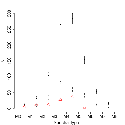
Figure 10: The distribution of spectral types in the 25 Orionis group. Triangles: confirmed members from this work and from Briceño et al. (2007). Black and empty dots indicate respectively the candidates in the entire area of the survey and inside the overdensity previously corrected by the expected contamination by field stars.

The system-IMF, and the spectral type distribution are commonly used as observables to constrain which processes and conditions are preponderant during the formation of LMS and BDs. In the sub-stellar domain some variations have been observed in these quantities, Taurus probably being the most representative case (Briceño et al., 2002). These variations are not well understood and more observations are needed in order to better constraint these phenomenon. What we have presented here is a new photometry-based system-IMF in the mass range $0.03<M/M_{\odot}<0.8$, obtained for a $\sim 7$ Myr old dispersed population in a low-density environment, using a numerous sample with 1246 objects. The peak of the spectral-types distribution and the characteristic mass $m_{c}$ of the log-normal representation of the system-IMF we found for the 25 Orionis group, is consistent with those reported for other SFR and young clusters (e.g. Oliveira, Jeffries & van Loon, 2009), which, as mentioned by Oliveira, Jeffries & van Loon (2009), supports the idea of an IMF relatively independent of environmental properties such as density, temperature, metallicity and radiation field, as predicted by the models from Bonnell, Clarke & Bate (2006) and Elmegreen, Klessen & Wilson (2008). On the other hand, the standard deviation $\sigma$ from the log-normal fit results to be slightly smaller than is expected from Chabrier (2003b) which is also consistent with the small values for the $\alpha_{3}$ coefficients obtained from the fit to a power-law IMF. This suggest that the 25 Orionis population could have a lower number of BDs. Because the fits are strongly dependent on small variations in the number of objects in the least massive bins, more observations are needed in order to better constraint the system-IMF in the sub-stellar domain of the 25 Orionis group and confirm such a trend. A sensitive photometric survey for the detection of a complete sample of BDs down to $\sim 0.01M_{\odot}$, and the spectroscopic confirmation of members in the entire mass range (including also $M>0.8M_{\odot}$) of this group are needed to confirm this low number of BD. Also, kinematic information is needed in order to evaluate whether the dynamical evolution of the group could be biasing the result. High spatial resolution imaging intended to detect binary or multiple systems are important in order to establish the effect that such a population of binaries could have on the observed system-IMF. Spectroscopic observations of our least massive candidates and much deeper photometric observations are currently under way.

5.2 The spatial distributions

Here we present the first comparative study of the spatial distribution of $\sim$1100 candidate LMS and $\sim$120 candidate BDs within the area covered by the 25 Orionis group and its surroundings. With this deep and spatially complete photometric sample we confirm the 25 Orionis group as the strong overdensity of stellar and sub-stellar candidate and members shown in Figure 11. We compute the number of objects on $3^{\prime}\times 3^{\prime}$ bins and smoothed the resulting pattern with a gaussian function with standard deviation of $6^{\prime}$ in both spatial directions. The overdensity is centred at $(\alpha,\delta)\sim(81\aas@@fstack{\circ}2,1\aas@@fstack{\circ}7)$ with a mean radius of $\sim 0\aas@@fstack{\circ}5$ and a slight elongation approximately in the East-West direction. Its mean density is of $\sim$0.5 objects per $3^{\prime}\times 3^{\prime}$ bin ($\sim 200obj/deg^{2}$), surrounded by a typical mean density of $\sim$0.25 objects per $3^{\prime}\times 3^{\prime}$ square ($\sim 100obj/deg^{2}$). The centre was computed as the position of the maximum density within the overdensity and the mean radius as the distance from the centre at which the density drops to the value of the mean density of the surroundings. Assuming a distance of $\sim$360 pc the angular radius corresponds to a mean linear radius of $\sim$3.14 pc. We note that the 25 Orionis overdensity appears to be superimposed on a low-density diagonal filament indicated in Figure 11, whose mean density is $\sim$0.3 objects per $3^{\prime}\times 3^{\prime}$ square.

The overdensities could be intrinsic to the population, a consequence of observational biases or a combination of both. We consider the detected overdensities as real because: (i) They are not a consequence of interstellar extinction, since the latter does not significantly affect the number of selected candidates and the SEM does not shows a spatial distribution similar with those from candidates, as can be seen in Figure 2. (ii) They cannot be explained as a consequence of contamination by field stars because these follow a smooth spatial distribution which depends on galactic latitude as predicted by the Besançon model. (iii) They are not a consequence of a photometric bias because the completeness and limiting magnitudes in all bands used for the candidate selection are spatially homogeneous in the area where the overdensities were detected and the slight difference in the completeness magnitude within observations centred at $\delta=1^{\circ}$ and $\delta=3^{\circ}$ (Table 2) cannot produce the detected overdensities. (iv) They are not a consequence of any artifact in the images or inappropriate identification of sources from different catalogues as we concluded from visual inspection of the images.

The East-West elongation of the 25 Orionis overdensity is suggested from the spatial distribution of the members confirmed by Briceño et al. (2005) and also by the spatial distribution of the high mass candidates of Kharchenko et al. (2005) with the highest probability of membership. In this work we confirm this trend with a numerous sample of well characterised candidates covering not only the 25 Orionis group but a reasonable area of its surroundings. Furthermore, our results rule out the idea of a possible extension of the 25 Orionis group to the South as suggested by McGehee (2006). With this new data set, deeper and covering the entire area surrounding the group, we find that the possible southern extension of the group reported by McGehee (2006) is probably part of the filament described above that extends also to the North-East direction, or the cluster ASCC18 from Kharchenko et al. (2005). This conclusion could not have been derived from the data considered by McGehee (2006), which covers only the southern part of the area shown in Figure 1. We note that the southern overdensity detected by McGehee (2006) at $(\alpha,\delta)\sim(81\aas@@fstack{\circ}2,0\aas@@fstack{\circ}8)$ is also observed in Figures 11 and 12 as part of the southern extension of the filament (note the different scales between our plots and Figure 8 from McGehee (2006)), but its mean low-density and position do not suggest it is part of the overdensity we consider here as the 25 Orionis group.

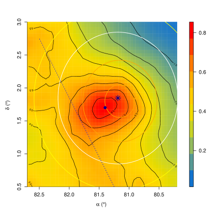
Figure 11: Spatial density distribution of the LMS and BD photometric candidates of the 25 Orionis group and its surroundings. Colored scales and isocontours indicate the mean density computed in bins of $3^{\prime}\times 3^{\prime}$ and smoothed with a gaussian with standard deviation of $6^{\prime}$ in both directions. The central strong overdensity is the 25 Orionis group and the doted line indicates the filamentary overdensity explained in the text. The circles indicate the radii from the previous works shown also in Figure 1. The contamination from field stars present in the candidate sample is spatially smooth. The central big dot indicates the centre of the group computed in this work, and the big asterisk, the position of the star 25 Ori.

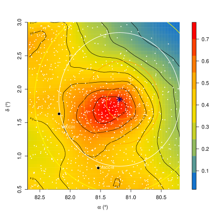
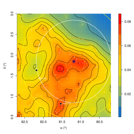
Figure 12: Comparison of the density distributions of LMS candidates ($M>0.08M_{\odot}$, white dots, left) and of BD candidates ($M<0.08M_{\odot}$, white dots, right). The K-S test probability between both distributions is 0.30 which indicates that both distributions are statistically indistinguishable. The big central asterisk represents the 25 Ori star and the black dots clusters from Kharchenko et al. (2005). Other elements are as in Figure 11.

Results from van den Bergh (2006) show that during their first $\sim$15 Myr, $\sim$20 per cent of galactic clusters and associations have diameters larger than 7 pc, being expanding associations rather than gravitationally bound clusters. Therefore the diameter obtained in this work for the 25 Orionis group (D$\sim$6.3 pc) suggests it could be a bound cluster given its age of about $\sim$7 Myr. Nevertheless, this computation is based on the radius found for the spatial overdensity, but we cannot rule out the cluster is spread over a larger area, since, as noted in Section 5.1, the age distribution and system-IMF are indistinguishable from its surroundings. A formal computation of the virial mass of this cluster is out of the scope of this work, since it depends almost entirely on its massive stars, which are not discussed here.

The panels of Figure 12 show separately the spatial density distribution of $\sim$1100 LMS and $\sim$120 BDs. In order to test whether the observed spatial distributions for BDs and LMS are drawn from the same parent distribution (null hypothesis), we have computed a two-dimensional two-sample Kolmogorov-Smirnov (K-S) test (Press et al., 2007). For the full BD and LMS samples the K-S statistic results in a probability $P=0.30$ of the null hypothesis being true, which means the difference between both spatial distributions is not statistically significant (Press et al., 2007). In order to assess the robustness of this result, we generated $10^{3}$ bootstrap resamples of both the BD and LMS distributions. A single bootstrap sample is made, e.g. for BDs, by randomly sampling with replacement from the BD catalogue, until a new set with the same number of objects (as the original catalogue) is generated. This is a standard technique that allows producing a set of random realizations drawn from the same distribution as the parent populations, which in this case are the BD and VLM samples (see e.g. Wall & Jenkins, 2012; Press et al., 2007, for more details). We computed the same K-S test on the $10^{3}$ bootstrap BD and LMS samples and found that only in 12 per cent of the experiments the distributions turned out to be incompatible at the 99 per cent confidence level ($P<0.01$). This shows it is a robust result, independent on stochastic fluctuations due to sample size, that the spatial distributions observed for BDs and LMS in this 7 Myr old population are statistically indistinguishable.

Although this result is not consistent with the mass segregation predicted by the early premature ejection models from Reipurth & Clarke (2001) subsequent work by Bate, Bonnell & Bromm (2003) does not predict significantly different velocity dispersions for ejected BDs and stars. Thus, the similar spatial distributions do not necessarily reject the premature ejection scenarios. In any case, what we are presenting here constitutes a new observational evidence supporting the similarity of the spatial distribution of LMS and BDs for a $\sim$7 Myr old population.

5.3 Disc indicators and accretion signatures

We computed the number fraction of LMS and BDs showing near IR excesses as an indication of the presence of primordial circumstellar inner-discs. In the left panel of Figure 13 we show a J-H vs. H-Ks colour-colour diagram with the CTTS locus from Meyer, Calvet & Hillenbrand (1997) and its extrapolation to M6 spectral type. We obtained that $3.8\pm 0.4$ per cent of LMS candidates and $4.5\pm 0.5$ per cent of spectroscopically confirmed LMS are placed inside the CTTS locus. Both results are in good agreement within the uncertainties and are consistent with those from Briceño et al. (2007) ($\sim 6$ per cent). The fractions reported here for the photometric candidates were computed considering the expected contamination by field stars and the errors were computed according to the binomial distribution.

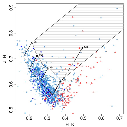
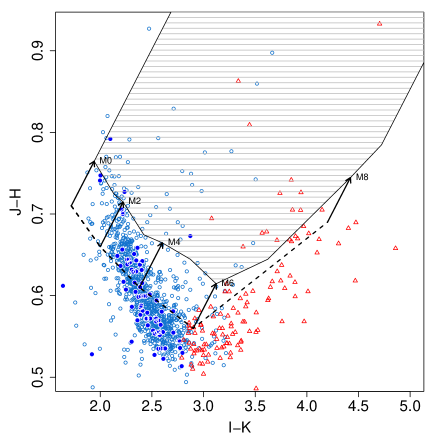
Figure 13: Optical and near-infrared colour-colour diagrams of spectroscopically confirmed members and photometric candidates. Left panel: J-H vs. H-Ks. Right panel: I-Ks vs. J-H. The dashed lines indicates the photospheric loci from Luhman et al. (2003b) and the shaded areas indicate the excess loci explained in Section 5.3. Empty and filled circles indicate respectively candidates and confirmed LMS. Triangles indicates candidate BDs. Reddening vectors for several spectral types are also indicated for the typical mean visual extinction ($A_{V}\sim 0.5$ mag) through the 25 Orionis group. Number fractions of objects showing IR-excesses are listed in Table 7.

Table 7: Number fraction of LMS and BDs showing infrared excesses.

Diagram	LMS members	LMS candidates	BD candidates
	[per cent]	[per cent]	[per cent]
J-H vs. H-Ks	$4.5\pm 0.5$	$3.8\pm 0.4$	$\cdots$
I-Ks vs. J-H	$4.1\pm 0.4$	$5.6\pm 0.5$	$12.7\pm 0.5$
3.6$\mu m$-4.5$\mu m$ vs. 4.5$\mu m$-5.8$\mu m$	$7.5\pm 0.4$	$7.8\pm 0.3$	$18.1\pm 0.3$
3.6$\mu m$-4.5$\mu m$ vs. 5.8$\mu m$-8.0$\mu m$	$12.0\pm 0.4$	$9.4\pm 0.8$	$39.2\pm 0.4$
Ks-8.0$\mu m$ vs. Ks-5.8$\mu m$	$5.7\pm 0.4$	$7.9\pm 0.5$	$47.0\pm 0.5$

For objects later than M6, the J-H vs. H-Ks diagram is not a good choice for detecting infrared excesses because the photospheric locus between spectral types M6 and M9 is essentially colinear with the corresponding reddenning vectors, which prevents a reliable measurement of the fraction of objects showing IR excesses as a function of their spectral-types. Because of this limitation, we apply an empirical criterion to detect objects with infrared excesses, using the I-Ks vs J-H diagram, where the photospheric loci and reddening vectors for spectral types between M6 and M9 are more separated, as we show in the right panel of Figure 13. Essentially we define a locus whose lower limit in the I-Ks vs J-H diagram is parallel to the photospheric locus from Luhman et al. (2003b), and which is separated from it by a distance equivalent to a reddening vector corresponding to $A_{V}=0.5$, which is slightly larger than the mean value of the interstellar extinction across the 25 Orionis group, as we have shown in Section 4.1. We found that $\sim 5.6\pm 0.5$ per cent of the candidate LMS and $\sim 4.1\pm 0.4$ per cent of the confirmed LMS show excesses. For the substellar regime the number fraction of candidates showing such IR excess is $12.7\pm 0.5$ per cent. Again, the number fraction of stars showing infrared excesses from inner discs agrees well with previous determinations by Hernández et al. (2006) and Briceño et al. (2007) using Spitzer data. In the sub-stellar regime, our result is the first estimate obtained for the 25 Orionis group.

Emissions from warm dust in evolved discs or in the external regions of primordial discs, occurs at longer wavelengths. In Figures 14 and 15 we show colour-colour diagrams in the wavelength range from $\sim 2.2\mu$m to $\sim 12\mu$m, for confirmed members and photometric candidates with magnitudes from VISTA, IRAC and WISE. The left panel of Figure 14 shows the 3.6$\mu$m-4.5$\mu$m vs. 4.5$\mu$m-5.8$\mu$m diagram from IRAC data with the excess region defined by Luhman et al. (2005) were $7.8\pm 0.3$ per cent of the candidates to LMS, $7.5\pm 0.4$ per cent of the LMS confirmed as members and $18.1\pm 0.3$ per cent of the candidates to BD show IR excesses. The right panel of Figure 14 shows the IRAC 3.6$\mu$m-4.5$\mu$m vs. 5.8$\mu$m-8.0$\mu$m diagram showing the CTTS locus defined by Hartmann et al. (2005) and Luhman et al. (2005), were $12.0\pm 0.4$ per cent of the LMS candidates, $9.4\pm 0.8$ per cent of the LMS confirmed as members and $39.2\pm 0.4$ per cent of the BD candidates show IR excesses.

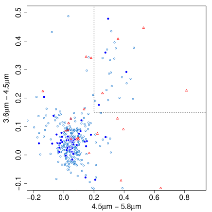
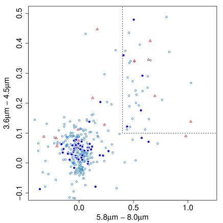
Figure 14: IRAC colour-colour diagrams of spectroscopically confirmed members and photometric candidates. Symbols are as in Figure 13. Left panel: the 3.6$\mu$m-4.5$\mu$m vs. 5.8$\mu$m-8.0$\mu$m diagram showing the CTTS locus (dashed lines) defined by Hartmann (2005). Right panel: the 3.6$\mu$m-4.5$\mu$m vs. 4.5$\mu$m-5.8$\mu$m diagrams with the excess region (dashed lines) defined by Luhman et al. (2005). Number fractions of objects showing IR-excesses are listed in Table 7

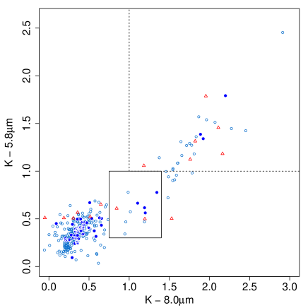
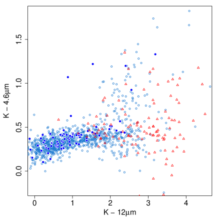
Figure 15: Color-colour diagram combining photometry from VISTA, IRAC and WISE. Symbols are as in Figure 13. Dashed polygons indicate disc loci and the solid polygon in the left panel encloses the possible transitional or evolved discs from the colour intervals defined by Luhman et al. (2010).

Using the Ks-8$\mu$m vs. Ks-24$\mu$m and the Ks-5.8$\mu$m vs. Ks-24$\mu$m diagrams based on IRAC and MIPS photometry, Luhman et al. (2010) show the distinction between circumstellar discs at different evolutionary stages. We do not have MIPS observations for the candidates and members considered in this work but we used the Ks-8$\mu$m and Ks-5.8$\mu$m colour intervals defined by Luhman et al. (2010) in order to separate objects showing photospheric emissions from those showing primordial discs and those showing transitional or evolved discs. Following this procedure we obtain an estimation of the number fraction of such populations. The left panel of Figure 15 shows the Ks-5.8$\mu$m vs. Ks-8.0$\mu$m diagram, where we consider objects with excesses to be those with Ks-5.8$\mu$m $>$ 1 and Ks-8.0$\mu$m $>$ 1, resulting in a number fraction of $7.9\pm 0.5$ per cent of the LMS candidates, $5.7\pm 0.4$ per cent for confirmed LMS and $\sim 47.0\pm 0.5$ per cent for the photometric candidates to BD. In the transitional and evolved disc locus, defined as the region between $0.75<Ks-8.0\mu m<1.4$ and $0.3<Ks-5.8\mu m<1$, we find 4 LMS members, 5 LMS candidates and 2 BD candidates for number fractions of $7.4\pm 0.4$ per cent, $2.3\pm 0.5$ per cent and $15.6\pm 0.5$ per cent respectively. The objects showing IR excesses indicative of possible transitional or evolved discs are listed in Table 8. In the right panel of Figure 15 we also show the excesses at longer wavelengths, using a Ks-4.6$\mu$m vs. Ks-12$\mu$m diagram from WISE data.

Table 8: Members and candidates showing possible transitional or evolved discs.

$\alpha(J2000)$	$\delta(J2000)$	J	I	CH1	CH2	CH3	CH4	W1	W2	W3	W4	ST	WHa	Av	Status
$[^{\circ}]$	$[^{\circ}]$												[$\AA$]	Av	Status
80.7117776526	1.51037395412	15.02	16.89	13.68	13.54	13.29	12.65	13.81	13.45	11.81	8.93	$\cdots$	$\cdots$	$\cdots$	Candidate
80.8808791321	2.22021102858	13.03	14.92	11.53	11.24	11.02	10.83	11.65	11.21	10.42	8.38	$\cdots$	$\cdots$	$\cdots$	Candidate
80.8829930224	2.17873892118	13.88	15.46	12.60	12.49	12.31	11.87	12.73	12.43	11.13	9.12	$\cdots$	$\cdots$	$\cdots$	Candidate
80.9343505087	1.69221474930	16.26	18.54	15.00	14.77	14.91	14.22	15.10	14.73	11.96	8.83	M1.0	-3.5	6.1	Member
81.0206640554	2.15769232385	14.48	16.47	13.10	12.87	12.59	12.06	13.33	12.85	11.54	8.31	$\cdots$	$\cdots$	$\cdots$	Candidate
81.1102509066	1.84858069829	14.81	16.55	13.59	13.50	13.39	12.82	13.76	13.57	11.72	8.76	M4.0	-2.1	1.1	Member
81.2452230354	1.42179289513	14.08	15.81	12.92	12.74	12.51	11.94	13.09	12.72	11.03	8.95	M5.0	-7.4	0.0	Member
81.3513507400	1.68539771614	13.78	15.61	12.56	12.44	12.32	11.88	12.77	12.47	10.99	8.72	M5.5	-15.1	0.0	Member
81.4447905792	1.72510889268	13.15	14.54	11.97	11.90	11.72	11.08	12.10	11.84	9.91	6.74	M3.5	-10.1	0.0	Member
81.4683299453	2.36818676306	13.16	14.52	11.27	10.97	10.82	10.58	11.38	10.96	9.88	8.10	$\cdots$	$\cdots$	$\cdots$	Candidate
81.5062304737	1.54283333334	14.71	16.42	13.31	13.12	12.91	12.45	13.64	13.31	11.47	9.16	$\cdots$	$\cdots$	$\cdots$	Candidate
81.6041933360	1.87740776106	15.28	17.08	13.99	13.91	13.71	13.50	14.18	13.91	12.18	8.47	M2.5	$\cdots$	2.8	Member
81.7246496737	2.30153351910	15.00	16.67	13.76	13.55	13.36	12.60	13.86	13.52	12.31	8.62	$\cdots$	$\cdots$	$\cdots$	Candidate
81.8506189547	1.63383891153	17.09	20.32	15.18	15.04	15.34	14.32	15.66	15.44	12.41	9.14	$\cdots$	$\cdots$	$\cdots$	Candidate
82.3184071926	2.15333352098	13.76	15.46	12.40	12.16	11.84	11.32	12.52	12.12	10.92	8.91	$\cdots$	$\cdots$	$\cdots$	Candidate
82.4413576233	1.95882675222	14.02	15.73	12.72	12.53	12.24	11.69	12.86	12.46	11.04	8.71	$\cdots$	$\cdots$	$\cdots$	Candidate
82.5921100764	1.64194791673	15.15	17.32	13.52	13.31	13.05	12.92	13.71	13.30	12.30	8.59	$\cdots$	$\cdots$	$\cdots$	Candidate

The samples of new confirmed members and candidates are not affected by the photometric completeness of the IRAC observations and the reported fractions are not biased towards the objects showing excesses. The number fraction of BD showing IR excesses turns out to be systematically higher in all colour-colour diagrams suggesting that at an age of $\sim 7$ Myr the disc fraction among BDs is larger than for LMS which could be an indicator of a slow evolution of discs around BDs. This supports previous results from Luhman & Mamajek (2012) for the Upper Scorpius association which with a estimated age of $\sim 11$Myr (Pecaut, Mamajek & Bubar, 2012) shows $\sim$25 per cent of objects later than M5 harbouring discs. Our results at a slight younger age support the scenario in which discs around LMS and BD evolve in different time scales in the sense that a higher fraction of BDs could retain their discs for longer periods of time.

Finally, low-resolution spectra provide an appropriate means to look for CTTS emission signatures such as H$\alpha$, the CaII triplet ($\lambda 8498$, $\lambda 8542$ and $\lambda 8662$) and HeI $\lambda 6676$. The dividing line between CTTS and weak (non-accreting) T-Tauri stars (WTTS) was first set in terms of the H$\alpha$ emission at W(H$\alpha$) $=-10$ Å by Herbig & Bell (1988). Afterwards, White & Basri (2003) revised this classification and, based on high resolution optical spectra ($R\sim 33000$), redefined the classification considering both the H$\alpha$ equivalent width and the spectral type. Barrado y Navascués & Martín (2003) using low-resolution optical spectra developed an empirical classification method based on the H$\alpha$ equivalent width and the spectral type. Here we followed the criteria from Barrado y Navascués & Martín (2003) to classify the confirmed LMS as CTTS or WTTS. Figure 16 shows the resulting classification in the $\rm W(H\alpha)$ vs. spectral-type plot. We obtained a number fraction of CTTS to WTTS of $3.8\pm 0.5$ per cent for objects earlier than M6. Our results are consistent with those from the colour-colour diagrams and with previous determinations by Briceño et al. (2005). On the other hand the number fraction of CTTS presented here is larger than the fraction reported by McGehee (2006) ($\sim 0.1$ per cent) that, as we explained in Section 5.2, most probably does not correspond to the 25 Orionis group.

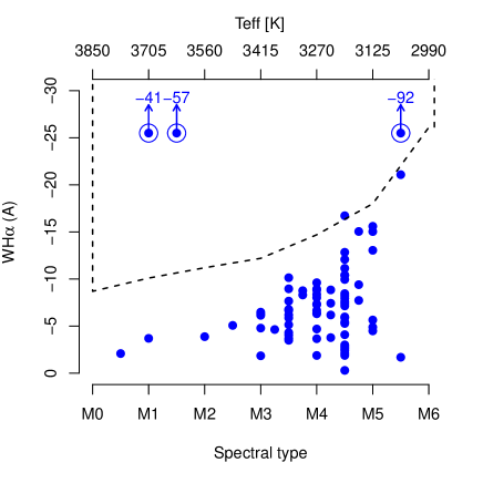
Figure 16: Equivalent width of $H\alpha$ versus spectral type and effective temperature (upper axis) for the new confirmed LMS members. Dotted lines indicate the limit between CTTS and WTTS according to Barrado y Navascués & Martín (2003). Circles indicates objects showing equivalent width of $H\alpha$ consistent with CTTS. Arrows indicate objects with strong $H\alpha$ emission whose $WH\alpha$ is labelled. We found 3.8 $\pm$ 0.5 per cent of the members of 25 Orionis group being CTTS (open circles).

6 Summary and conclusions

We have presented the first extensive study of the lower mass population ($0.02\leq M/M_{\odot}\leq 0.8$) of the 25 Ori group and its surrounding regions. We provide for this mass range the spatial distribution, mean age, IMF, and investigate the presence of circumstellar discs and accretion signatures. In the following we summarize our results:

• We have obtained a sample of 1246 photometric candidates to LMS and BDs in the 25 Ori group and its surroundings with estimated masses within $0.02\raisebox{-2.15277pt}{$\,\stackrel{{\scriptstyle\textstyle<}}{{\sim}}\,$}M/M_{\odot}\raisebox{-2.15277pt}{$\,\stackrel{{\scriptstyle\textstyle<}}{{\sim}}\,$}0.8$, as well as 77 new LMS spectroscopically confirmed as members with spectral types in the range $\sim$M1 to $\sim$M5.

• We have characterised the possible contamination of our photometric candidate sample using the Besançon Galactic model (Robin et al., 2003). The expected mean contamination was found to be $\sim 33$ field dwarf stars from the foreground per $deg^{2}$, which yields an expected average efficiency of $\sim 82$ per cent for our photometric candidate selection.

• From the age distributions of the photometric candidates and confirmed members we find mean ages of $7.7\pm 0.6$ Myr and $6.1\pm 0.8$ Myr respectively. These results are in good agreement with those reported by Briceño et al. (2005).

• We have derived the system-IMF for 25 Ori from a numerous sample of photometric candidate LMS and BDs previously corrected by the contamination from field stars. We have obtained a system-IMF which can be well described by either a Kroupa power-law function with indices $\alpha_{3}=-1.73\pm 0.31$ and $\alpha_{2}=0.68\pm 0.41$ in the mass ranges $0.03<M/M_{\odot}<0.08$ and $0.08<M/M_{\odot}<0.5$ respectively, or a Scalo log-normal function with coefficients $m_{c}=0.21^{+0.02}_{-0.02}$ and $\sigma=0.36\pm 0.02$ in the mass range $0.03<M/M_{\odot}<0.8$. For the log-normal representation of the IMF we obtained that the characteristic mass is consistent with an IMF independent of environmental properties, although the standard deviation is smaller than the system-IMF from Chabrier (2003a). A sensitive photometric survey for the detection of a complete sample of BD down to $\sim 0.01M\odot$, and their spectroscopic counterparts is needed to confirm the slightly lower value of the standard deviation and whether this trend of the system-IMF is a consequence of a real deficit of BDs.

• From the analysis of the spatial distribution of the photometric candidate sample we find the peak of the 25 Orionis overdensity at $(\alpha,\delta)\sim(81\aas@@fstack{\circ}2,1\aas@@fstack{\circ}7)$ with a diameter of $\sim 6.3$ pc. We have confirmed the East-West elongation of the 25 Orionis group, also observed in the works from Kharchenko et al. (2005) and Briceño et al. (2005), and rule out the southern extension proposed by McGehee (2006). Additionally we found that the 25 Orionis group is projected over a filament distributed along the south-west to north-east direction. We have also found that the spatial distributions of LMS and BDs in 25 Orionis are statistically indistinguishable.

• For the LMS we calculated the number fraction of stars showing IR excess in the J-H vs H-Ks diagram according to the CTTS locus from Meyer, Calvet & Hillenbrand (1997). We found that $\sim 4$ per cent of the LMS show the levels of IR excess expected from CTTS with optically thick primordial discs. We found similar fractions for the empirical locus defined in the $I-Ks$ vs $J-H$ colour-colour diagram where we find also that $\sim 12$ per cent of the BD show IR excesses indicative of primordial discs.

• Using VISTA, IRAC and WISE photometry we have also found IR excess at longer wavelengths indicative of discs. Depending on the selected diagram we found that the number fraction of LMS showing IR excesses is between $\sim$7 to $\sim$10 per cent while the number fraction for BDs increases up to $\sim$20 to $\sim$50 per cent.

• Additionally we found that 11 members and candidates show signs of possible transitional or evolved discs and that $3.8\pm 0.5$ per cent of the LMS members show $H\alpha$ emission consistent with a CTTS nature, confirming the CTTS number fraction found by Briceño et al. (2007).

• Our results show that the fraction of BD showing IR excesses is higher than for LMS, supporting the scenario in which the evolution of circumstellar discs around the least massive stars could occur at larger time scales.

References

- Abazajian et al. (2005) Abazajian K. et al., 2005, AJ, 129, 1755
- Baltay et al. (2002) Baltay C. et al., 2002, PASP, 114, 780
- Baraffe et al. (1998) Baraffe I., Chabrier G., Allard F., Hauschildt P. H., 1998, A&A, 337, 403
- Barrado y Navascués & Martín (2003) Barrado y Navascués D., Martín E. L., 2003, AJ, 126, 2997
- Basri (1998) Basri G., 1998, in Astronomical Society of the Pacific Conference Series, Vol. 134, Brown Dwarfs and Extrasolar Planets, R. Rebolo, E. L. Martin, & M. R. Zapatero Osorio, pp. 394–+
- Bastian, Covey & Meyer (2010) Bastian N., Covey K. R., Meyer M. R., 2010, ARA&A, 48, 339
- Bate, Bonnell & Bromm (2003) Bate M. R., Bonnell I. A., Bromm V., 2003, MNRAS, 339, 577
- Biazzo et al. (2011) Biazzo K., Randich S., Palla F., Briceño C., 2011, A&A, 530, A19+
- Bonnell, Clarke & Bate (2006) Bonnell I. A., Clarke C. J., Bate M. R., 2006, MNRAS, 368, 1296
- Boudreault & Bailer-Jones (2009) Boudreault S., Bailer-Jones C. A. L., 2009, ApJ, 706, 1484
- Bouvier et al. (2008) Bouvier J. et al., 2008, A&A, 481, 661
- Briceño et al. (2005) Briceño C., Calvet N., Hernández J., Vivas A. K., Hartmann L., Downes J. J., Berlind P., 2005, AJ, 129, 907
- Briceño et al. (2007) Briceño C., Hartmann L., Hernández J., Calvet N., Vivas A. K., Furesz G., Szentgyorgyi A., 2007, ApJ, 661, 1119
- Briceño et al. (1998) Briceño C., Hartmann L., Stauffer J., Martín E., 1998, AJ, 115, 2074
- Briceño et al. (2002) Briceño C., Luhman K. L., Hartmann L., Stauffer J. R., Kirkpatrick J. D., 2002, ApJ, 580, 317
- Briceño et al. (2001) Briceño C. et al., 2001, Science, 291, 93
- Calvet et al. (2005) Calvet N., Briceño C., Hernández J., Hoyer S., Hartmann L., Sicilia-Aguilar A., Megeath S. T., D’Alessio P., 2005, AJ, 129, 935
- Cardelli, Clayton & Mathis (1989) Cardelli J. A., Clayton G. C., Mathis J. S., 1989, ApJ, 345, 245
- Caswell (2007) Caswell J. L., 2007, in IAU Symposium, Vol. 242, IAU Symposium, J. M. Chapman & W. A. Baan, ed., pp. 194–199
- Chabrier (2003a) Chabrier G., 2003a, PASP, 115, 763
- Chabrier (2003b) Chabrier G., 2003b, ApJL, 586, L133
- Chabrier et al. (2005) Chabrier G., Baraffe I., Allard F., Hauschildt P. H., 2005, ArXiv Astrophysics e-prints
- Chen & Lee (2008) Chen W. P., Lee H. T., 2008, arXiv.org, astro-ph, to appear in the Handbook of Star Forming Regions, Vol. I, edited byBo Reipurth
- Dahm (2008) Dahm S. E., 2008, The Young Cluster and Star Forming Region NGC 2264, Reipurth, B., ed., pp. 966–+
- Dahn et al. (2002) Dahn C. C. et al., 2002, AJ, 124, 1170
- Davenport et al. (2006) Davenport J. R. A., West A. A., Matthiesen C. K., Schmieding M., Kobelski A., 2006, PASP, 118, 1679
- Downes et al. (2008) Downes J. J., Briceño C., Hernández J., Calvet N., Hartmann L., Ponsot Balaguer E., 2008, AJ, 136, 51
- Dullemond & Dominik (2004) Dullemond C. P., Dominik C., 2004, A&A, 421, 1075
- Elmegreen, Klessen & Wilson (2008) Elmegreen B. G., Klessen R. S., Wilson C. D., 2008, ApJ, 681, 365
- Emerson & Sutherland (2010) Emerson J. P., Sutherland W. J., 2010, in Society of Photo-Optical Instrumentation Engineers (SPIE) Conference Series, Vol. 7733, Society of Photo-Optical Instrumentation Engineers (SPIE) Conference Series
- Emerson et al. (2004) Emerson J. P., Sutherland W. J., McPherson A. M., Craig S. C., Dalton G. B., Ward A. K., 2004, The Messenger, 117, 27
- Fabricant et al. (2005) Fabricant D. et al., 2005, PASP, 117, 1411
- Hartmann (2001) Hartmann L., 2001, AJ, 121, 1030
- Hartmann (2005) Hartmann L., 2005, in Astronomical Society of the Pacific Conference Series, Vol. 341, Chondrites and the Protoplanetary Disk, A. N. Krot, E. R. D. Scott, & B. Reipurth, ed., pp. 131–+
- Hartmann et al. (2005) Hartmann L., Megeath S. T., Allen L., Luhman K., Calvet N., D’Alessio P., Franco-Hernandez R., Fazio G., 2005, ApJ, 629, 881
- Herbig & Bell (1988) Herbig G. H., Bell K. R., 1988, Third Catalog of Emission-Line Stars of the Orion Population : 3 : 1988, Herbig, G. H. & Bell, K. R., ed.
- Hernández et al. (2006) Hernández J., Briceño C., Calvet N., Hartmann L., Muzerolle J., Quintero A., 2006, ApJ, 652, 472
- Hernández et al. (2004) Hernández J., Calvet N., Briceño C., Hartmann L., Berlind P., 2004, AJ, 127, 1682
- Hernández et al. (2007) Hernández J. et al., 2007, ApJ, 671, 1784
- Hernández et al. (2008) Hernández J., Hartmann L., Calvet N., Jeffries R. D., Gutermuth R., Muzerolle J., Stauffer J., 2008, ApJ, 686, 1195
- Hodgkin et al. (2009) Hodgkin S. T., Irwin M. J., Hewett P. C., Warren S. J., 2009, MNRAS, 394, 675
- Ingleby et al. (2011) Ingleby L., Calvet N., Hernández J., Briceño C., Espaillat C., Miller J., Bergin E., Hartmann L., 2011, AJ, 141, 127
- Jayawardhana, Mohanty & Basri (2003) Jayawardhana R., Mohanty S., Basri G., 2003, ApJ, 592, 282
- Jeffries et al. (2007) Jeffries R. D., Oliveira J. M., Naylor T., Mayne N. J., Littlefair S. P., 2007, MNRAS, 376, 580
- Joergens (2006) Joergens V., 2006, A&A, 446, 1165
- Kharchenko et al. (2005) Kharchenko N. V., Piskunov A. E., Röser S., Schilbach E., Scholz R., 2005, A&A, 440, 403
- Kirkpatrick et al. (1999) Kirkpatrick J. D. et al., 1999, ApJ, 519, 802
- Kraus, White & Hillenbrand (2006) Kraus A. L., White R. J., Hillenbrand L. A., 2006, ApJ, 649, 306
- Kroupa (2001) Kroupa P., 2001, MNRAS, 322, 231
- Kroupa (2002) Kroupa P., 2002, Science, 295, 82
- Kumar & Schmeja (2007) Kumar M. S. N., Schmeja S., 2007, A&A, 471, L33
- Kun, Kiss & Balog (2008) Kun M., Kiss Z. T., Balog Z., 2008, Star Forming Regions in Cepheus, Reipurth, B., ed., pp. 136–+
- Landolt (1992) Landolt A. U., 1992, AJ, 104, 340
- Lodieu et al. (2007) Lodieu N., Hambly N. C., Jameson R. F., Hodgkin S. T., Carraro G., Kendall T. R., 2007, MNRAS, 374, 372
- Luhman (2004) Luhman K. L., 2004, ApJ, 614, 398
- Luhman (2012) Luhman K. L., 2012, ARA&A, 50, 65
- Luhman et al. (2010) Luhman K. L., Allen P. R., Espaillat C., Hartmann L., Calvet N., 2010, ApJS, 186, 111
- Luhman et al. (2003a) Luhman K. L., Briceño C., Stauffer J. R., Hartmann L., Barrado y Navascués D., Caldwell N., 2003a, ApJ, 590, 348
- Luhman et al. (2007) Luhman K. L., Joergens V., Lada C., Muzerolle J., Pascucci I., White R., 2007, Protostars and Planets V, 443
- Luhman et al. (2005) Luhman K. L. et al., 2005, ApJL, 631, L69
- Luhman & Mamajek (2012) Luhman K. L., Mamajek E. E., 2012, ApJ, 758, 31
- Luhman et al. (2009) Luhman K. L., Mamajek E. E., Allen P. R., Muench A. A., Finkbeiner D. P., 2009, ApJ, 691, 1265
- Luhman et al. (2003b) Luhman K. L., Stauffer J. R., Muench A. A., Rieke G. H., Lada E. A., Bouvier J., Lada C. J., 2003b, ApJ, 593, 1093
- Mateu et al. (2012) Mateu C., Vivas A. K., Downes J. J., Briceño C., Zinn R., Cruz-Diaz G., 2012, MNRAS, 427, 3374
- McCarthy & Zuckerman (2004) McCarthy C., Zuckerman B., 2004, AJ, 127, 2871
- McGehee (2006) McGehee P. M., 2006, AJ, 131, 2959
- Meyer, Calvet & Hillenbrand (1997) Meyer M. R., Calvet N., Hillenbrand L. A., 1997, AJ, 114, 288
- Mink (2006) Mink D., 2006, in Astronomical Society of the Pacific Conference Series, Vol. 351, Astronomical Data Analysis Software and Systems XV, C. Gabriel, C. Arviset, D. Ponz, & S. Enrique, ed., p. 204
- Monet (1998) Monet D. G., 1998, in Bulletin of the American Astronomical Society, Vol. 30, Bulletin of the American Astronomical Society, pp. 1427–+
- Muzerolle et al. (2000) Muzerolle J., Briceño C., Calvet N., Hartmann L., Hillenbrand L., Gullbring E., 2000, ApJL, 545, L141
- Muzerolle et al. (2005) Muzerolle J., Luhman K. L., Briceño C., Hartmann L., Calvet N., 2005, ApJ, 625, 906
- Neuhäuser et al. (2011) Neuhäuser R. et al., 2011, Astronomische Nachrichten, 332, 547
- Oliveira, Jeffries & van Loon (2009) Oliveira J. M., Jeffries R. D., van Loon J. T., 2009, MNRAS, 392, 1034
- Padoan & Nordlund (2004) Padoan P., Nordlund Å., 2004, ApJ, 617, 559
- Parravano, McKee & Hollenbach (2010) Parravano A., McKee C. F., Hollenbach D., 2010, 45
- Pecaut, Mamajek & Bubar (2012) Pecaut M. J., Mamajek E. E., Bubar E. J., 2012, ApJ, 746, 154
- Petr-Gotzens et al. (2011) Petr-Gotzens M. et al., 2011, The Messenger, 145, 29
- Preibisch (2012) Preibisch T., 2012, Research in Astronomy and Astrophysics, 12, 1, provided by the SAO/NASA Astrophysics Data System
- Press et al. (2007) Press W. H., Teukolsky S. A., Vetterling W. T., Flannery B. P., 2007, Numerical recipes in C, Cambridge University Press
- Reipurth & Clarke (2001) Reipurth B., Clarke C., 2001, AJ, 122, 432
- Robin et al. (2003) Robin A. C., Reylé C., Derrière S., Picaud S., 2003, A&A, 409, 523
- Scalo (1986) Scalo J. M., 1986, FCP, 11, 1
- Schlegel, Finkbeiner & Davis (1998) Schlegel D. J., Finkbeiner D. P., Davis M., 1998, ApJ, 500, 525
- Scholz & Eislöffel (2005) Scholz A., Eislöffel J., 2005, A&A, 429, 1007
- Scholz et al. (2009) Scholz A., Xu X., Jayawardhana R., Wood K., Eislöffel J., Quinn C., 2009, MNRAS, 398, 873
- Skrutskie et al. (2006) Skrutskie M. F. et al., 2006, AJ, 131, 1163
- Strom et al. (1989) Strom K. M., Wilkin F. P., Strom S. E., Seaman R. L., 1989, AJ, 98, 1444
- Taylor (2006) Taylor M. B., 2006, in Astronomical Society of the Pacific Conference Series, Vol. 351, Astronomical Data Analysis Software and Systems XV, C. Gabriel, C. Arviset, D. Ponz, & S. Enrique, ed., p. 666
- Torres et al. (2008) Torres C. A. O., Quast G. R., Melo C. H. F., Sterzik M. F., 2008, Young Nearby Loose Associations, Reipurth, B., pp. 757–+
- van den Bergh (2006) van den Bergh S., 2006, AJ, 131, 1559
- van Eyken et al. (2011) van Eyken J. C. et al., 2011, AJ, 142, 60
- Wall & Jenkins (2012) Wall J. V., Jenkins C. R., 2012, Practical Statistics for Astronomers
- Weidenschilling (1997) Weidenschilling S. J., 1997, ICARUS, 127, 290
- White & Basri (2003) White R. J., Basri G., 2003, ApJ, 582, 1109
- Whitworth et al. (2007) Whitworth A., Bate M. R., Nordlund Å., Reipurth B., Zinnecker H., 2007, Protostars and Planets V, 999, 459
- Wright et al. (2010) Wright E. L. et al., 2010, AJ, 140, 1868