On the equilibrium of rotating filaments

Abstract

The physical properties of the so-called Ostriker isothermal, non-rotating filament have been classically used as benchmark to interpret the stability of the filaments observed in nearby clouds. However, such static picture seems to contrast with the more dynamical state observed in different filaments. In order to explore the physical conditions of filaments under realistic conditions, in this work we theoretically investigate how the equilibrium structure of a filament changes in a rotating configuration. To do so, we solve the hydrostatic equilibrium equation assuming both uniform and differential rotations independently. We obtain a new set of equilibrium solutions for rotating and pressure truncated filaments. These new equilibrium solutions are found to present both radial and projected column density profiles shallower than their Ostriker-like counterparts. Moreover, and for rotational periods similar to those found in the observations, the centrifugal forces present in these filaments are also able to sustain large amounts of mass (larger than the mass attained by the Ostriker filament) without being necessary unstable. Our results indicate that further analysis on the physical state of star-forming filaments should take into account rotational effects as stabilizing agents against gravity

1 Introduction

Although the observations of filaments within molecular clouds have been reported since decades (e.g. Schneider & Elmegreen 1979), only recently their presence has been recognized as a unique characteristic of the star-formation process. The latest Herschel results have revealed the direct connection between the filaments, dense cores and stars in all kinds of environments along the Milky Way, from low-mass and nearby clouds (André et al. 2010) to most distant and high-mass star-forming regions (Molinari et al. 2010). As a consequence, characterizing the physical properties of these filaments has been revealed as key to our understanding of the origin of the stars within molecular clouds.

The large majority of observational papers (Arzoumanian et al. 2011; Palmeirim et al. 2013; Hacar et al. 2013) use the classical “Ostriker” profile (Ostriker 1964) as a benchmark to interpret observations. More specifically, if the estimated linear mass of an observed filament is larger than the value obtained for the Ostriker filament ($\simeq$ 16.6 M_⊙ pc^-1 for T=10 K), it is assumed that the filament is unstable. Analogously, density profiles flatter than the Ostriker profile are generally interpreted as a a sign of collapse. However, it is worth recalling the assumptions and limitations of this model: $(i)$ filaments are assumed to be isothermal, $(ii)$ they are not rotating, $(iii)$ they are isolated, $(iv)$ they can be modeled as cylindrical structures with infinite length, $(v)$ their support against gravity comes solely from thermal pressure. An increasing number of observational results suggest however that none of the above assumptions can be considered as strictly valid. In a first paper (Recchi et al. 2013, hereafter Paper I) we have relaxed the hypothesis $(i)$ and we have considered equilibrium structures of non-isothermal filaments. Concerning hypothesis $(ii)$, and after the pioneering work of Robe (1968), there has been a number of publications devoted to the study of equilibrium and stability of rotating filaments (see e.g. Hansen et al. 1976; Inagaki & Hachisu 1978; Robe 1979; Simon et al. 1981; Veugelen 1985; Horedt 2004; Kaur et al. 2006; Oproiu & Horedt 2008). However, this body of knowledge has not been recently used to constrain properties of observed filaments in molecular clouds. In this work we aim to explore the effects of rotation on the interpretation of the physical state of filaments during the formation of dense cores and stars. Moreover, we emphasize the role of envelopes on the determination of density profiles, an aspect often overlooked in the recent literature.

The paper is organised as follows. In Sect. 2 we review the observational evidences suggesting that star-forming filaments are rotating. In Sect. 3 we study the equilibrium configuration of rotating filaments and the results of our calculations are discussed and compared with available observations. Finally, in Sect. 4 some conclusions are drawn.

2 Observational signs of rotation in filaments

Since the first millimeter studies in nearby clouds it is well known that star-forming filaments present complex motions both parallel and perpendicular to their main axis (e.g. Loren 1989; Uchida et al. 1991). Recently, Hacar & Tafalla (2011) have shown that the internal dynamical structure of the so-called velocity coherent filaments is dominated by the presence of local motions, typically characterized by velocity gradients of the order of 1.5–2.0 km s^-1 pc^-1, similar to those found inside dense cores (e.g. Caselli et al. 2002). Comparing the structure of both density and velocity perturbations along the main axis of different filaments, Hacar & Tafalla (2011) identified the periodicity of different longitudinal modes as the streaming motions leading to the formation of dense cores within these objects. These authors also noticed the presence of distinct and non-parallel components with similar amplitudes than their longitudinal counterparts. Interpreted as rotational modes, these perpendicular motions would correspond to a maximum angular frequency $\omega$ of about 6.5 $\cdot$ 10^-14 s^-1. Assuming these values as characteristic defining the rotational frequency in Galactic filaments, the detection of such rotational levels then rises the question on whether they could potentially influence the stability of these objects.

To estimate the dynamical relevance of rotation we can take the total kinetic energy per unit length as equal to $\mathcal{T}=\frac{1}{2}\omega^{2}R_{c}^{2}M_{lin}$, where $R_{c}$ is the external radius of the cylinder and $M_{lin}$ its linear mass. The total gravitational energy per unit mass is $W=G{M_{lin}}^{2}$, hence the ratio $\mathcal{T}/W$ is

$$\frac{\mathcal{T}}{W}\simeq 0.65\left(\frac{\omega}{6.5\cdot 10^{-14}}\right)^{2}\left(\frac{R_{c}}{0.15\,{\rm pc}}\right)^{2}\left(\frac{M_{lin}}{16.6\,{\rm M}_{\odot}\,{\rm pc}^{-1}}\right)^{-1}.$$ (1)

Clearly, for nominal values of $\omega$, $R_{c}$ and $M_{lin}$ the total kinetic energy associated to rotation is significant, thus rotation is dynamically important.

3 The equilibrium configuration of rotating, non-isothermal filaments

In order to calculate the density distribution of rotating, non-isothermal filaments, we extend the approach already used in Paper I, which we shortly repeat here. The starting equation is the hydrostatic equilibrium with rotation: $\nabla P=\rho(g+\omega^{2}r)$. We introduce the normalization:

$$\rho=\theta\rho_{0},\;\;T=\tau T_{0},\;\;r=Hx\;\;\Omega=\sqrt{\frac{2}{\pi G\rho_{0}}}\omega.$$ (2)

Here, $\rho_{0}$ and $T_{0}$ are the central density and temperature, respectively, $H=\sqrt{\frac{2kT_{0}}{\pi G\rho_{0}\mu m_{H}}}$ is a length scale and $\Omega$ is a normalized frequency. Simple steps transform the hydrostatic equilibrium equation into:

$$\theta\tau^{\prime}+\tau\theta^{\prime}=\theta\left(\Omega^{2}x-8\frac{\int_{0}^{x}{\tilde{x}}\theta d{\tilde{x}}}{x}\right).$$ (3)

Calling now $I=\int_{0}^{x}{\tilde{x}}\theta d{\tilde{x}}$, then clearly $I^{\prime}=\theta x$. Solving the above equation for $I$, we obtain $8I=\Omega^{2}x^{2}-\tau^{\prime}x-\tau x\frac{\theta^{\prime}}{\theta}$. Upon differentiating this expression with respect to $x$ and rearranging, we obtain:

$$\theta^{\prime\prime}=\frac{\left(\theta^{\prime}\right)^{2}}{\theta}-\theta^{\prime}\left[\frac{\tau^{\prime}}{\tau}+\frac{1}{x}\right]-\frac{\theta}{\tau}\left[\tau^{\prime\prime}+\frac{\tau^{\prime}}{x}+8\theta-2\Omega^{2}-2x\Omega\Omega^{\prime}\right].$$ (4)

Correctly, for $\Omega=0$ we recover the equation already used in Paper I. This second-order differential equation, together with the boundary conditions $\theta(0)=1$, $\theta^{\prime}(0)=-\tau^{\prime}(0)$ (see Paper I) can be integrated numerically to obtain equilibrium configurations of both rotating and non-isothermal filaments independently. This expression is more convenient than classical Lane-Emden type equations (see e.g. Robe 1968; Hansen et al. 1976) for the problem at hand. Notice also that also the normalization of $\omega$ differs from the more conventional assumption $\eta^{2}=\omega^{2}/4\pi G\rho_{0}$ (Hansen et al. 1976).

3.1 Uniformly rotating filaments

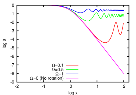
Figure 1: Logarithm of the normalized density $\theta$ as a function of $x$ for various models of isothermal filaments with different normalized angular frequencies. The model with $\Omega=0$ corresponds to the Ostriker profile with $\rho\propto r^{-4}$ at large radii.

If we set $\tau,\Omega=Const$ in Eq. 4, we can obtain equilibrium solutions for isothermal, uniformly rotating filaments. We have checked that our numerical results reproduce the main features of this kind of cylinders, already known in the literature, namely:

• Density inversions take place for $\Omega^{2}>0$ as the centrifugal, gravitational and pressure gradient forces battle to maintain mechanical equilibrium. Density oscillations occur in other equilibrium distributions of polytropes (see Horedt 2004 for a very comprehensive overview). Noticeably, the equilibrium solution of uniformly rotating cylindrical polytropes with polytropic index $n=1$ depends on the (oscillating) zeroth-order Bessel function $J_{0}$ (Robe 1968; see also Christodoulou & Kazanas 2007). Solutions for rotating cylindrical polytropes with $n>1$ maintain this oscillating character although they can not be expressed analytically. As evident in Fig. 1, in the case of isothermal cylinders (corresponding to $n\rightarrow\infty$), the frequency of oscillations is zero for $\Omega=0$, corresponding to the Ostriker profile. This frequency increases with the angular frequency $\Omega$.

• For $\Omega>2$, $\rho^{\prime}(0)>0$, due to the fact that, in this case, the effective gravity $g+\omega^{2}r$ is directed outwards. For $\Omega<2$, $\rho^{\prime}(0)<0$. If $\Omega=2$, there is perfect equilibrium between centrifugal and gravitational forces (Keplerian rotation) and the density is constant (see also Inagaki & Hachisu 1978).

• The density tends asymptotically to the value $\Omega^{2}/4$. This implies also that the integrated mass per unit length $\Pi=\int_{0}^{\infty}2\pi x\theta(x)dx$ diverges for $\Omega^{2}>0$. Rotating filaments must be thus pressure truncated. This limit of $\theta$ for large values of $x$ is essentially the reason why density oscillations arise for $\Omega\neq 2$. This limit can not be reached smoothly, i.e. the density gradient can not tend to zero. If the density gradient tends to zero, so does the pressure gradient. In this case there must be asymptotically a perfect equilibrium between gravity and centrifugal force (Keplerian rotation) but, as we have noticed above, this equilibrium is possible only if $\Omega=2$. Thanks to the density oscillations, $\nabla P$ does not tend to zero and perfect Keplerian rotation is never attained. Notice moreover that the divergence of the linear mass is a consequence of the fact that the centrifugal force diverges, too, for $x\rightarrow\infty$.

All these features can be recognized in Fig. 1, where the logarithm of the normalized density $\theta$ is plotted as a function of the filament radius $x$ for models with various angular frequencies $\Omega$, ranging from 0 (non-rotating Ostriker filament) to 1. Hansen et al. (1976) performed a stability analysis of uniformly rotating isothermal cylinders, based on a standard linear perturbation of the hydrodynamical equations. They noticed that, beyond the point where the first density inversion occurs, the system behaves differently compared to the non-rotation case. Dynamically unstable oscillation modes appear and the cylinder tends to form spiral structures. Notice that a more extended stability analysis, not limited to isothermal or uniformly rotating cylinders, has been recently performed by Freundlich et al. (2014; see also Breysse et al. 2014).

Even in its simplest form, the inclusion of rotations has interesting consequences in the interpretation of the physical state of filaments. As discussed in Paper I, the properties of the Ostriker filament (Stodólkiewicz 1963; Ostriker 1964), in particular its radial profile and linear mass, are classically used to discern the stability of these structures. According to the Ostriker solution, an infinite and isothermal filament in hydrostatic equilibrium presents an internal density distribution that tends to $\rho(r)\propto r^{-4}$ at large radii and a linear mass M${}_{Ost}\simeq 16.6$ M_⊙ pc^-1 at 10 K. As shown in Fig. 1, and ought to the effects of the centrifugal force, the radial profile of an uniformly rotating filament in equilibrium ($\Omega>0$) could present much shallower profiles than in the Ostriker-like configuration (i.e. $\Omega=0$). Such departure from the Ostriker profile is translated into a variation of the linear mass that can be supported by these rotating systems. For comparison, an estimation of the linear masses for different rotating filaments in equilibrium truncated at a normalized radius x=3 and x=10 are presented in Tables 1 and 2, respectively. In these tables, the temperature profile is the linear function $\tau(x)=1+Ax$. In particular, the case $A=0$ refers to isothermal filaments, whereas if $A>0$, the temperature is increasing outwards. As can be seen there, the linear mass of a rotating filament could easily exceed the critical linear mass of its Ostriker-like counterpart without being necessary unstable.

It is also instructive to obtain estimations of the above models in physical units in order to interpret observations in nearby clouds. For typical filaments similar to those found in Taurus (Hacar & Tafalla 2011; Palmeirim et al. 2013; Hacar et al. 2013), with central densities of $\sim 5\cdot 10^{4}$ cm^-3, one obtains $\Omega\simeq 0.5$ according to Eq. 2. Assuming a temperature of 10 K, and from Tables 1 and 2 (case $A=0$), this rotation level leads to an increase in the linear mass between $\sim$ 17.4 M_⊙ pc^-1 if the filament is truncated at radius x=3, and up to $\sim$ 112 M_⊙ pc^-1 for truncation radius of x=10. Here, it is worth noticing that a normalized frequency of $\Omega\simeq 0.5$, or $\omega\sim 6.5\cdot 10^{-14}$ s^-1, corresponds to a rotation period of $\sim$ 3.1 Myr. With probably less than one revolution in their entire lifetimes ($\tau\sim$ 1–2 Myr), the centrifugal forces inside such slow rotating filaments can then provide a non-negligible support against their gravitational collapse, being able to sustain larger masses than in the case of an isothermal and static Ostriker-like filament.

3.2 Differentially rotating filaments

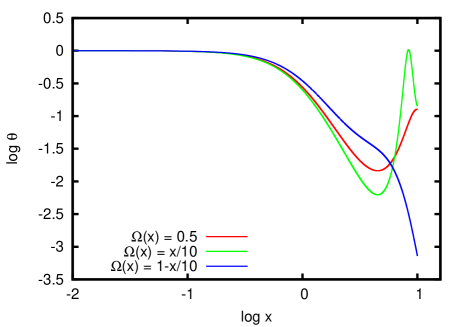
Figure 2: Logarithm of the normalized density $\theta$ as a function of $x$ for various models of filaments with different rotation laws.

As can be noticed in Fig. 1, a distinct signature of the centrifugal forces acting within rotating filaments is the presence of secondary peaks (i.e. density inversions) in their radial density distribution at large radii. Such density inversions could dynamically detach the outer layers of the filament to its central region, eventually leading to the mechanical breaking of these structures. In Sect. 3.1, we assumed that the filaments present a uniform rotation, similar to solid bodies. However, our limited information concerning the the rotation profiles in real filaments invites to explore other rotation configurations.

Table 1: Normalized linear masses at $x=3$ compared to the Ostriker filament with similar truncation radius, with M${}_{Ost}(x\leq 3)=14.9$ M_⊙ pc^-1, as a function of $\Omega$ and $A$.

$\Omega$	$A=0$	$A=0.02$	$A=0.1$	$A=0.5$
0.1	1.006	1.015	1.049	1.167
0.5	1.166	1.176	1.213	1.330
0.8	1.553	1.561	1.593	1.676
1.0	2.108	2.108	2.111	2.117

Table 2: Similar to Table 1 but for linear masses at $x=10$, with M${}_{Ost}(x\leq 10)=16.4$ M_⊙ pc^-1.

$\Omega$	$A=0$	$A=0.02$	$A=0.1$	$A=0.5$
0.1	1.015	1.039	1.137	1.623
0.2	1.075	1.102	1.212	1.730
0.3	1.287	1.309	1.415	1.951
0.4	2.533	2.321	2.063	2.379
0.5	7.019	6.347	4.377	3.234
0.6	10.37	10.53	9.398	4.988
0.7	12.29	12.77	13.78	8.399
0.8	14.96	15.14	16.59	13.84
0.9	20.05	19.39	19.43	20.22
1.0	26.22	25.70	23.71	25.95

For the sake of simplicity, we have investigated the equilibrium configuration of filaments presenting differential rotation, assuming that $\Omega$ linearly varies with the filament radius $x$. For illustrative purposes, we choose two simple laws: $\Omega_{1}(x)=x/10$ and $\Omega_{2}(x)=1-x/10$, both attaining the typical frequency $\Omega=0.5$ at $x=5$. The first of these laws presumes that the filament rotates faster at larger radii but presents no rotation at the axis, resembling a shear motion. Opposite to it, the second one assumes that the filament presents its maximum angular speed at the axis and that it radially decreases outwards.

The comparison of the resulting density profiles for these two models presented above are shown in Fig. 2 for normalized radii x$\leq$ 10. For comparison, there we also overplot the density profile obtained with a constant frequency $\Omega=0.5$ (see Sect. 3.1). For these models, we are assuming A=0, i.e. isothermal configurations. Clearly, the law $\Omega_{1}(x)$ displays a radial profile with even stronger oscillations than the model with uniform rotation. As mentioned above, oscillations are prone to dynamical instabilities. In this case, instabilities start occurring at the minimum of the density distribution, here located at $x\simeq 4.45$. Conversely, these density oscillations are suppressed in rotating filaments that obey a law like $\Omega_{2}(x)$. It is however worth noticing that this last rotational law fails to satisfy the Solberg-Høiland criterion for stability against axisymmetric perturbations (Tassoul 1978; Endal & Sofia 1978; Horedt 2004). Stability can be discussed by evaluating the first order derivative $\frac{d}{dx}[x^{4}\Omega^{2}_{2}(x)]$, which is positive for $x\in(0,20/3)\cup(10,+\infty)$ and negative for $x\in(20/3,10)$. We must therefore either consider that this filament is unstable at large radii, or we must assume it to be pressure-truncated at radii smaller than x=20/3 $\simeq$ 6.7. As we mentioned above, we could not exclude the hypothesis that rotation indeed induced instability and fragmentation of the original filament, separating the central part (at radii x$\;\buildrel<\over{\sim}\;$ 4.45 for $\Omega=\Omega_{1}(x)$ and x$\;\buildrel<\over{\sim}\;$ 6.7 for $\Omega=\Omega_{2}(x)$) from the outer mantel, which might subsequently break into smaller units. This (speculative) picture would be consistent with the bundle of filaments observed in B213 (Hacar et al. 2013). For comparison, the mass per unit length attained by the model with $\Omega=\Omega_{1}(x)$ at $x<4.45$ (which corresponds to $\sim$ 0.2 pc for $T=10$ K and $n_{c}\sim 5\cdot 10^{4}$ cm^-3) is equal to 0.99 M_Ost whereas the mass outside this minimum is equal to 22.7 M_Ost, i.e. there is enough mass to form many other filaments.

3.3 Non-isothermal and rotating filaments

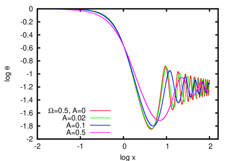
Figure 3: Logarithm of the normalized density $\theta$ as a function of $x$ for various models of uniformly rotating filaments with $\Omega=0.5$ and different temperature slopes $A$.

As demonstrated in Paper I, the presence of internal temperature gradients within filaments could offer an additional support against gravity. Under realistic conditions, these thermal effects should be then considered in combination to different rotational modes in the study of the stability of these objects.

The numerical solutions obtained for the equilibrium configuration of filaments with $\Omega=0.5$ and various values of $A$ are plotted in Fig. 3. Notice that Fig. 5 of Palmeirim et al. (2013) suggests a rather shallower dust temperature gradient with a value of A of the order of 0.02 (green curve in Fig. 3). However, as discussed in Paper I, the gas temperature profile could be steeper than the dust one, so it is useful to consider also larger values of $A$. Fig. 3 shows that the asymptotic behaviour of the solution does not depend on $A$: $\theta(x)$ always tends to $\Omega^{2}/4$ for $x\rightarrow\infty$. By looking at Eq. 4, it is clear that the same asymptotic behaviour holds for a wide range of reasonable temperature and frequency profiles. Whenever $\tau^{\prime\prime}$, $\tau^{\prime}/x$ and $\Omega\Omega^{\prime}x$ tend to zero for $x\rightarrow\infty$, and this condition holds for a linear increasing $\tau(x)$ and for $\Omega=$constant, the asymptotic value of $\theta(x)$ is $\Omega^{2}/4$. It is easy to see that also the asymptotically constant law fulfils this condition if the angular frequency is constant.

Figure 3 also shows that density oscillations are damped in the presence of positive temperature gradients. This was expected as more pressure is provided to the external layers to contrast the effect of the centrifugal force. Since density inversions are dynamically unstable, positive temperature gradients must be thus seen as a stabilizing mechanism in filaments. Our numerical calculations indicate in addition that the inclusion of temperature variations also increases the amount of mass that can be supported in rotating filaments. This effect is again quantified in Tables 1 and 2 for truncation radii of $x=3$ and $x=10$, respectively, compared to the linear mass obtained for an Ostriker profile at the same radius. As can be seen there, the expected linear masses are always larger than in the isothermal and non-rotating filaments, although the exact value depends on the combination of $\Omega$ and $A$ due to the variation in the position of the secondary density peaks compared to the truncation radius.

3.4 Derived column densities for non-isothermal, rotating filaments: isolated vs. embedded configurations

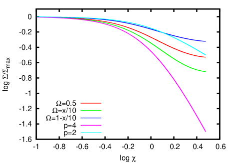
Figure 4: Column density, as a function of the normalized impact parameter $\chi$, for filaments characterized by three different rotation laws: increasing outwards ($\Omega=x/10$), decreasing outwards ($\Omega=1-x/10$) and constant ($\Omega=0.5$). The filament is embedded in a cylindrical molecular cloud, with radius five times the radius of the filament. The column density of the Ostriker filament (case $p=4$) and the one obtained for a Plummer-like model with $\rho\sim r^{-2}$ (case $p=2$) are also shown for comparison.

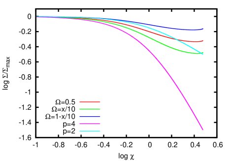
Figure 5: Same as Fig. 4 but for a filament embedded in a slab, with half-thickness five times the radius of the filament.

In addition to their radial profiles, we also calculated the column density profiles produced by these non-isothermal, rotating filaments in equilibrium presented in previous sections, as a critical parameter to compare with the observations. For the case of isolated filaments, the total column density at different impact parameters $\chi$ can be directly calculated integrating (either analytically or numerically) their density profiles along the line of sight. As a general rule, if the volume density $\rho$ is proportional to $r^{-p}$, then the column density $\Sigma(\chi)$ is proportional to $\chi^{1-p}$. This result holds not only for both Ostriker filaments (see also Appendix A) and more general Plummer-like profiles (e.g. see Eq. 1 in Arzoumanian et al. 2011), but also also for the new rotating, non-isothermal configurations explored in this paper. Recent observations seem to indicate that those filaments typically found in molecular clouds present column density profiles with $\Sigma(\chi)\sim\chi^{-1}$, i.e. $p\simeq 2$ (see Arzoumanian et al. 2011; Palmeirim et al. 2013), a value that we use for comparison hereafter.

An aspect often underestimated in the literature is the influence of the filament envelope in the determination of column densities profiles. Particularly if a filament is embedded in (and pressure-truncated by) a large molecular cloud, the line of sight also intercepts some cloud material whose contribution to the column density could be non-negligible (see also Appendix A), as previously suggested by different observational and theoretical studies (e.g. Stepnik et al. 2003; Juvela et al. 2012). In order to quantify the influence of the ambient gas in the determination of the column densities, here we consider two prototypical cases:

1. The filament is embedded in a co-axial cylindrical molecular cloud with radius $R_{m}$.

2. The filament is embedded in a sheet with half-thickness $R_{m}$.

Note that, if the filament is not located in the plane of the sky, the quantity that enters the calculation of the column density is not $R_{m}$ itself, but $R_{m}^{\prime}=R_{m}/\cos\beta$, where $\beta$ is the angle between the axis of the filament and this plane.

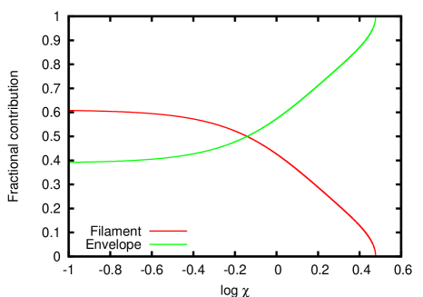
Figure 6: Fractional contribution of filament and envelope to the total column density. The model shown here corresponds to the blue line of Fig. 4: the rotation profile is $\Omega=1-x/10$ and the filament is surrounded by a cylindrical envelope with R_m/R_c=5.

Following the results presented in Sect. 3.1-3.3, we have investigated the observational properties of three representative filaments in equilibrium obeying different rotational laws, namely $\Omega_{1}(x)=x/10$, $\Omega_{2}(x)=1-x/10$ and $\Omega_{3}(x)=0.5$, covering both differential and uniform rotational patterns. The contribution of the envelope to the observed column densities is obviously determined by its relative depth compared to the truncation radius of the filament as well as the shape of its envelope. To illustrate this behaviour, we have first assumed that these filaments are pressure-truncated at $x=3$ (a conservative estimate). Moreover, we have considered these filaments to be embedded into the two different cloud configurations presented before, that is a slab and a cylinder, both with extensions $R_{m}$ corresponding to five times the radius of the filament (i.e. R_m/R${}_{c}=5$). In both cases, we have assumed that the density of the envelope is constant and equal to the filament density at its truncation radius i.e. at $x=3$.

The recovered column densities for the models presented above as a function of the impact parameter $\chi$ in the case of the two cylindrical and slab geometries are shown in Figs. 4 and 5, respectively. In both cases, the impact parameter $\chi$ is measured in units of $H$. The results obtained there are compared with the expected column densities in the case of two infinite filaments described by an Ostriker-like profile (case $p=4$) and a Plummer-like profile with $\rho\propto r^{-2}$ at large radii (case $p=2$), as suggested by observations. From these comparisons it is clear that all the explored configurations present shallower profiles than the expected column density for its equivalent Ostriker-like filament. This is due to the constant value of the density in the envelope, which tends to wash out the density gradient present in the filament if the envelope radius is large. Moreover, the column densities expected for embedded filaments described by rotating laws like $\Omega_{1}(x)$ and $\Omega_{3}(x)$ (this last one only if the filament embedded into a slab) exhibit a radial dependency even shallower than these p=2 models at large impact parameters. The relative contribution of filament and envelope is outlined in Fig. 6. The model shown here corresponds to the blue line of Fig. 4: the rotation profile is $\Omega=1-x/10$ and the filament is surrounded by a cylindrical envelope with R_m/R_c=5. As expected, at larger projected radii the observed radial profiles are entirely determined by the total column density of the cloud.

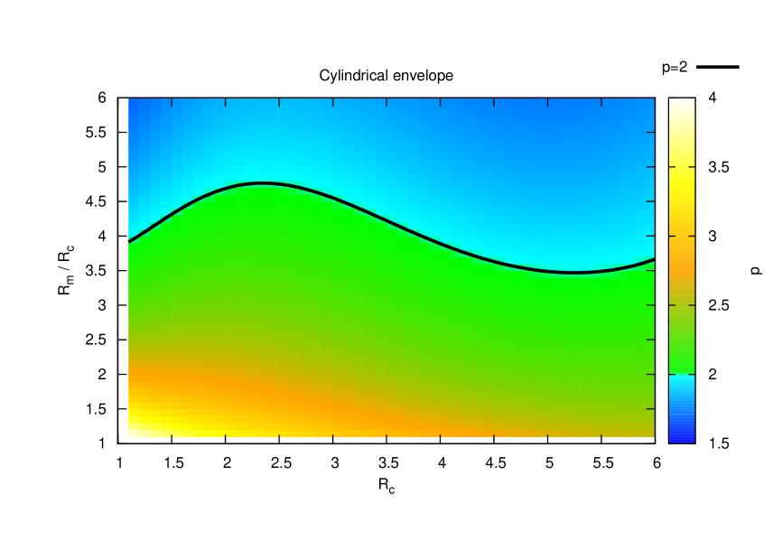
Figure 7: Expected radial dependence for the observed column density profiles (colour coded) of rotating filaments in equilibrium obeying a rotation law like $\Omega_{2}(x)=1-x/10$, truncated at a radius R_c, and embedded into a cylindrical cloud extending up to a distance R_m. R_c and R_m are displayed in units of the normalized (i.e. x) and truncation (i.e. R_m/R_c) radii, respectively. The black solid line highlights those models with a power-law dependence with p=2, similar to the observations. Notice that also the color palette has been chosen in order to emphasize the transition from $p<2$ configurations to $p>2$ configurations.

Finally, it is important to remark that the expected column density profiles for the models presented above and, particularly, their agreement to these shallow Plummer-like profiles with p=2, significantly depend on the selection of the truncation radius R_c and the extent of the filament envelopes R_m. This fact is illustrated in Fig. 7 exploring the expected slope of the observed column density profiles for pressure truncated and isothermal filaments following a rotational law like $\Omega_{2}(x)=1-x/10$ under different configurations for both their truncation and cloud radii. These results were calculated as the averaged value of the local slope of the column density at impact parameters $\chi\leq R_{c}$, that is, where our models are sensitive to the distinct contributions of both filaments and envelopes. As expected, the larger the cloud depth is compared to the filament, the flatter profile is expected. Within the range of values explored in the figure, multiple combinations for both R_c and R_m parameters present slopes consistent to a power-law like dependency with p=2. Although less prominently, few additional combinations can be also obtained in the case of filaments with rotational laws like $\Omega_{1}(x)=x/10$ or $\Omega_{3}(x)=0.5$ (not shown here). Unless the rotational state of a filament is known and the contribution of the cloud background is properly evaluated, such degeneration between the parameters defining the cloud geometry and the relative weights of both the filament and its envelope makes inconclusive any stability analysis solely based on its mass radial distribution.

4 Conclusions

The results presented this paper have explored whether the inclusion of different rotational patterns affect the stability of gaseous filaments similar to those observed in nearby clouds. Our numerical results show that, even in configurations involving slow rotations, the presence of centrifugal forces have a stabilizing effect, effectively sustaining large amounts of gas against the gravitational collapse of these objects. These centrifugal forces promote however the formation of density inversions that are dynamically unstable at large radii, making the inner parts of these rotating filaments to detach from their outermost layers. To prevent the formation of these instabilities as well as the asymptotical increase of their linear masses at large radii, any equilibrium configuration for these rotating filaments would require them to be pressure truncated at relatively low radii.

In order to have a proper comparison with observations, we have also computed the expected column density profiles for different pressure truncated, rotating filaments in equilibrium. To reproduce their profiles under realistic conditions we have also considered these filaments to be embedded in an homogeneous cloud with different geometries. According to our calculations, the predicted column density profiles for such rotating filaments and their envelopes tend to produce much shallower profiles than those expected for the case of Ostriker-like filaments, resembling the results found in observations of nearby clouds. Unfortunately, we found that different combinations of rotating configurations and envelopes could reproduce these observed of profiles, complicating this comparison.

To conclude, the stability of an observed filament can not be judged by a simple comparison between observations and the predictions of the Ostriker profile. We have shown in this paper that density profiles much flatter than the Ostriker profile and linear masses significantly larger than the canonical value of $\simeq$ 16.6 M_⊙ pc^-1 can be obtained for rotating filaments in equilibrium, surrounded by an envelope. Detailed descriptions of the filament kinematics and their rotational state, in addition to the analysis of their projected column densities distributions, are therefore needed to evaluate the stability and physical state in these objects.

Appendix A On the column density of filaments embedded in molecular clouds

In this appendix we derive a formula to calculate the column density of filaments embedded in large molecular clouds. For that, let us assume first the general case of an isothermal filament described by the Ostriker solution $\theta_{i}(x)=\left[1+x^{2}\right]^{-2}$. If we call $z$ the (normalized) distance between the plane in the sky where the filament is located and a generic plane, then the distance between the point $(\chi,z)$ (where $\chi$ is the normalized impact parameter) and the axis is simply $x=\sqrt{\chi^{2}+z^{2}}$. As it is well known, if we assume that the filament extends until infinite distances, then the column density is:

$$\Sigma(\chi) =\int_{-\infty}^{\infty}\theta_{i}(\chi,z)dz=\int_{-\infty}^{\infty}\frac{dz}{(1+z^{2}+\chi^{2})^{2}}$$

$$=\frac{1}{2}\frac{\pi}{(\chi^{2}+1)^{3/2}}.$$ (5)

However, the cylinder could be embedded in a more extended cloud, with radius $R_{m}$. If we take for simplicity the cloud aligned with the filament, the situation is shown in Fig. 8.

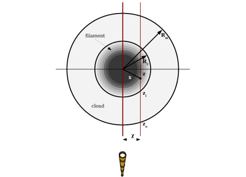
Figure 8: Section of the filament (with radius $R_{c}$), embedded in a (cylindrical, co-axial) molecular cloud with radius $R_{m}$.

Based on this figure (and due to the symmetry of the problem), we can write the column density as:

$$\Sigma(\chi)=2\int_{0}^{z_{o}}\theta_{i}(\chi,z)dz=2\int_{z_{o}}^{z_{i}}\theta_{b}dz+2\int_{0}^{z_{i}}\frac{dz}{(1+z^{2}+\chi^{2})^{2}}.$$ (6)

Here we have defined (see also Fig. 8):

$$z_{o}=\sqrt{R_{m}^{2}-\chi^{2}},\;\;\;\;z_{i}=\sqrt{R_{c}^{2}-\chi^{2}},\;\;\;\;\theta_{b}=\theta(R_{c}),$$ (7)

and assumed that the density of the molecular cloud is constant and equal to $\theta(R_{c})$. The result is:

$$\Sigma(\chi) =2\theta_{b}(z_{o}-z_{i})+\frac{z_{i}}{(\chi^{2}+1)(R_{c}^{2}+1)}+\frac{\tan^{-1}\sqrt{\frac{R_{c}^{2}-\chi^{2}}{\chi^{2}+1}}}{(\chi^{2}+1)^{3/2}},$$

$$=2\frac{\sqrt{R_{m}^{2}-\chi^{2}}-\sqrt{R_{c}^{2}-\chi^{2}}}{(1+R_{c}^{2})^{2}}+\frac{\sqrt{R_{c}^{2}-\chi^{2}}}{(\chi^{2}+1)(R_{c}^{2}+1)}+$$

$$+\frac{\tan^{-1}\sqrt{\frac{R_{c}^{2}-\chi^{2}}{\chi^{2}+1}}}{(\chi^{2}+1)^{3/2}}.$$ (8)

It is easy to see that, in the limes for $R_{c}$ (and $R_{m}$) tending to infinity, we recover the column density profile found above for the infinite cylinder.

Another possibility is to assume that the cylinder is immersed in a slab of gas with half thickness $R_{m}$. The derivation of the column density remains the same and the only difference is that $z_{o}$ is now fix (it is equal to $R_{m}$) and does not depend any more on $\chi$ as before.

For filaments whose profiles are determined numerically (like the ones found in Sect. 3) the integral:

$$\int_{0}^{z_{i}}\theta(\chi,z)dz,$$ (9)

(where as usual $\chi$ and $z$ are related to $x$ by $x=\sqrt{\chi^{2}+z^{2}}$) must be calculated numerically. The contribution to the column density due to the surrounding molecular cloud remains unaltered.

References

- [] André, P., Men’shchikov, A., Bontemps, S., et al. 2010, A&A, 518, L102
- [] Arzoumanian, D., André, P., Didelon, P., et al. 2011, A&A, 529, L6
- [] Breysse, P. C., Kamionkowski, M., & Benson, A. 2014, MNRAS, 437, 2675
- [] Caselli, P., Benson, P. J., Myers, P. C., & Tafalla, M. 2002, ApJ, 572, 238
- [] Christodoulou, D. M., & Kazanas, D. 2007, arXiv:0706.3205
- [] Endal, A. S., & Sofia, S. 1978, ApJ, 220, 279
- [] Freundlich, J., Jog, C. J., & Combes, F. 2014, A&A, 564, A7
- [] Hacar, A., & Tafalla, M. 2011, A&A, 533, A34
- [] Hacar, A., Tafalla, M., Kauffmann, J., & Kovacs, A. 2013, A&A, 554, A55
- [] Hansen, C. J., Aizenman, M. L., & Ross, R. L. 1976, ApJ, 207, 736
- [] Horedt, G. P. 2004, Polytropes - Applications in Astrophysics and Related Fields, Astrophysics and Space Science Library, 306
- [] Inagaki, S., & Hachisu, I. 1978, PASJ, 30, 39
- [] Juvela, M., Malinen, J., & Lunttila, T. 2012, A&A, 544, A141
- [] Kaur, A., Sood, N. K., Singh, L., & Singh, K. D. 2006, Ap&SS, 301, 89
- [] Loren, R. B. 1989, ApJ, 338, 925
- [] Molinari, S., Swinyard, B., Bally, J., et al. 2010, A&A, 518, L100
- [] Oproiu, T., & Horedt, G. P. 2008, ApJ, 688, 1112
- [] Ostriker, J. 1964, ApJ, 140, 1056
- [] Palmeirim, P., André, P., Kirk, J., et al. 2013, A&A, 550, A38
- [] Recchi, S., Hacar, A., Palestini, A. 2013, A&A, 558, A27 (Paper I)
- [] Robe, H. 1968, Annales d’Astrophysique, 31, 549
- [] Robe, H. 1979, A&A, 75, 14
- [] Schneider, S., & Elmegreen, B. G. 1979, ApJS, 41, 87
- [] Simon, S. A., Czysz, M. F., Everett, K., & Field, C. 1981, American Journal of Physics, 49, 662
- [] Stepnik, B., Abergel, A., Bernard, J.-P., et al. 2003, A&A, 398, 551
- [] Stodólkiewicz, J. S. 1963, Acta Astronomica, 13, 30
- [] Tassoul, J.-L. 1978, Princeton Series in Astrophysics, Princeton: University Press, 1978,
- [] Uchida, Y., Fukui, Y., Minoshima, Y., Mizuno, A., & Iwata, T. 1991, Nature, 349, 140
- [] Veugelen, P. 1985, Ap&SS, 109, 45